The Generalized Lasso Problem and Uniqueness

Abstract

We study uniqueness in the generalized lasso problem, where the penalty is the $\ell_{1}$ norm of a matrix $D$ times the coefficient vector. We derive a broad result on uniqueness that places weak assumptions on the predictor matrix $X$ and penalty matrix $D$; the implication is that, if $D$ is fixed and its null space is not too large (the dimension of its null space is at most the number of samples), and $X$ and response vector $y$ jointly follow an absolutely continuous distribution, then the generalized lasso problem has a unique solution almost surely, regardless of the number of predictors relative to the number of samples. This effectively generalizes previous uniqueness results for the lasso problem (Tibshirani, 2013) (which corresponds to the special case $D=I$). Further, we extend our study to the case in which the loss is given by the negative log-likelihood from a generalized linear model. In addition to uniqueness results, we derive results on the local stability of generalized lasso solutions that might be of interest in their own right.

1 Introduction

We consider the generalized lasso problem

$$\mathop{\mathrm{minimize}}_{\beta\in\mathbb{R}^{p}}\;\frac{1}{2}\|y-X\beta\|_{2}^{2}+\lambda\|D\beta\|_{1},$$ (1)

where $y\in\mathbb{R}^{n}$ is a response vector, $X\in\mathbb{R}^{n\times p}$ is a predictor matrix, $D\in\mathbb{R}^{m\times p}$ is a penalty matrix, and $\lambda\geq 0$ is a tuning parameter. As explained in Tibshirani and Taylor (2011), the generalized lasso problem (1) encompasses several well-studied problems as special cases, corresponding to different choices of $D$, e.g., the lasso (Tibshirani, 1996), the fused lasso (Rudin et al., 1992; Tibshirani et al., 2005), trend filtering (Steidl et al., 2006; Kim et al., 2009), the graph fused lasso (Hoefling, 2010), graph trend filtering (Wang et al., 2016), Kronecker trend filtering (Sadhanala et al., 2017), among others. (For all problems except the lasso problem, the literature is mainly focused on the so-called “signal approximator” case, where $X=I$, and the responses have a certain underlying structure; but the “regression” case, where $X$ is arbitrary, naturally arises whenever the predictor variables—rather than the responses—have an analogous structure.)

There has been an abundance of theoretical and computational work on the generalized lasso and its special cases. In the current paper, we examine sufficient conditions under which the solution in (1) will be unique. While this is simple enough to state, it is a problem of fundamental importance. The generalized lasso has been used as a modeling tool in numerous application areas, such as copy number variation analysis (Tibshirani and Wang, 2008), sMRI image classification (Xin et al., 2014), evolutionary shift detection on phylogenetic trees, (Khabbazian et al., 2016), motion-capture tracking (Madrid-Padilla and Scott, 2017), and longitudinal prediction of disease progression (Adhikari et al., 2019). In such applications, the structure of the solution $\hat{\beta}$ in hand (found by using one of many optimization methods applicable to (1), a convex quadratic program) usually carries meaning—this is because $D$ has been carefully chosen so that sparsity in $D\hat{\beta}$ translates into some interesting and domain-appropriate structure for $\hat{\beta}$. Of course, nonuniqueness of the solution in (1) would cause complications in interpreting this structure. (The practitioner would be left wondering: are there other solutions providing compementary, or even contradictory structures?) Further, beyond interpretation, nonuniqueness of the generalized lasso solution would clearly cause complications if we are seeking to use this solution to make predictions (via $x^{T}\hat{\beta}$, for a new predictor vector $x\in\mathbb{R}^{p}$), as different solutions would lead to different predictions (potentially very different ones).

When $p\leq n$ and $\mathrm{rank}(X)=p$, there is always a unique solution in (1) due to strict convexity of the squared loss term. Our focus will thus be in deriving sufficient conditions for uniqueness in the high-dimensional case, where $\mathrm{rank}(X)<p$. It also worth noting that when $\mathrm{null}(X)\cap\mathrm{null}(D)\neq\{0\}$ problem (1) cannot have a unique solution. (If $\eta\neq 0$ lies in this intersection, and $\hat{\beta}$ is a solution in (1), then so will be $\hat{\beta}+\eta$.) Therefore, at the very least, any sufficient condition for uniqueness in (1) must include (or imply) the null space condition $\mathrm{null}(X)\cap\mathrm{null}(D)=\{0\}$.

In the lasso problem, defined by taking $D=I$ in (1), several authors have studied conditions for uniqueness, notably Tibshirani (2013), who showed that when the entries of $X$ are drawn from an arbitrary continuous distribution, the lasso solution is unique almost surely. One of the main results in this paper yields this lasso result as a special case; see Theorem 1, and Remark 5 following the theorem. Moreover, our study of uniqueness leads us to develop intermediate properties of generalized lasso solutions that may be of interest in their own right—in particular, when we broaden our focus to a version of (1) in which the squared loss is replaced by a general loss function, we derive local stability properties of solutions that have potential applications beyond this paper.

In the remainder of this introduction, we describe the implications of our uniqueness results for various special cases of the generalized lasso, discuss related work, and then cover notation and an outline of the rest of the paper.

1.1 Uniqueness in special cases

The following is an application of Theorem 1 to various special cases for the penalty matrix $D$. The takeaway is that, for continuously distributed predictors and responses, uniqueness can be ensured almost surely in various interesting cases of the generalized lasso, provided that $n$ is not “too small”, meaning that the sample size $n$ is at least the nullity (dimension of the null space) of $D$. (Some of the cases presented in the corollary can be folded into others, but we list them anyway for clarity.)

Corollary 1.

Fix any $\lambda>0$. Assume the joint distribution of $(X,y)$ is absolutely continuous with respect to $(np+n)$-dimensional Lebesgue measure. Then problem (1) admits a unique solution almost surely, in any one of the following cases:

1. $D=I\in\mathbb{R}^{p\times p}$ is the identity matrix;

2. $D\in\mathbb{R}^{(p-1)\times p}$ is the first difference matrix, i.e., fused lasso penalty matrix (see Section 2.1.1 in Tibshirani and Taylor (2011));

3. $D\in\mathbb{R}^{(p-k-1)\times p}$ is the $(k+1)$st order difference matrix, i.e., $k$th order trend filtering penalty matrix (see Section 2.1.2 in Tibshirani and Taylor (2011)), and $n\geq k+1$;

4. $D\in\mathbb{R}^{m\times p}$ is the graph fused lasso penalty matrix, defined over a graph with $m$ edges, $n$ nodes, and $r$ connected components (see Section 2.1.1 in Tibshirani and Taylor (2011)), and $n\geq r$;

5. $D\in\mathbb{R}^{m\times p}$ is the $k$th order graph trend filtering penalty matrix, defined over a graph with $m$ edges, $n$ nodes, and $r$ connected components (see Wang et al. (2016)), and $n\geq r$;

6. $D\in\mathbb{R}^{(N-k-1)N^{d-1}d\times N^{d}}$ is the $k$th order Kronecker trend filtering penalty matrix, defined over a $d$-dimensional grid graph with all equal side lengths $N=n^{1/d}$ (see Sadhanala et al. (2017)), and $n\geq(k+1)^{d}$.

Two interesting special cases of the generalized lasso that fall outside the scope of our results here are additive trend filtering (Sadhanala and Tibshirani, 2017) and varying-coefficient models (which can be cast in a generalized lasso form, see Section 2.2 of Tibshirani and Taylor (2011)). In either of these problems, the predictor matrix $X$ has random elements but obeys a particular structure, thus it is not reasonable to assume that its entries overall follow a continuous distribution, so Theorem 1 cannot be immediately applied. Still, we believe that under weak conditions either problem should have a unique solution. Sadhanala and Tibshirani (2017) give a uniqueness result for additive trend filtering by reducing this problem to lasso form; but, keeping this problem in generalized lasso form and carefully investigating an application of Lemma 6 (the deterministic result in this paper leading to Theorem 1) may yield a result with simpler sufficient conditions. This is left to future work.

Furthermore, by applying Theorem 2 to various special cases for $D$, analogous results hold (for all cases in Corollary 1) when the squared loss is replaced by a generalized linear model (GLM) loss $G$ as in (19). In this setting, the assumption that $(X,y)$ is jointly absolutely continuous is replaced by the two assumptions that $X$ is absolutely continous, and $y\notin\mathcal{N}$, where $\mathcal{N}$ is the set defined in (41). The set $\mathcal{N}$ has Lebesgue measure zero for some common choices of loss $G$ (see Remark 12); but unless we somewhat artificially assume that the distribution of $y|X$ is continuous (this is artificial because in the two most fundamental GLMs outside of the Gaussian model, namely the Bernoulli and Poisson models, the entries of $y|X$ are discrete), the fact that $\mathcal{N}$ has Lebesgue measure zero set does not directly imply that the condition $y\notin\mathcal{N}$ holds almost surely. Still, it seems that $y\notin\mathcal{N}$ should be “likely”—and hence, uniqueness should be “likely”—in a typical GLM setup, and making this precise is left to future work.

1.2 Related work

Several authors have examined uniqueness of solutions in statistical optimization problems en route to proving risk or recovery properties of these solutions; see Donoho (2006); Dossal (2012) for examples of this in the noiseless lasso problem (and the analogous noiseless $\ell_{0}$ penalized problem); see Nam et al. (2013) for an example in the noiseless generalized lasso problem; see Fuchs (2005); Candes and Plan (2009); Wainwright (2009) for examples in the lasso problem; and lastly, see Lee et al. (2015) for an example in the generalized lasso problem. These results have a different aim than ours, i.e., their main goal—a risk or recovery guarantee—is more ambitious than certifying uniqueness alone, and thus the conditions they require are more stringent. Our work in this paper is more along the lines of direct uniqueness analysis in the lasso, as was carried out by Osborne et al. (2000); Rosset et al. (2004); Tibshirani (2013); Schneider and Ewald (2017).

1.3 Notation and outline

In terms of notation, for a matrix $A\in\mathbb{R}^{m\times n}$, we write $A^{+}$ for its Moore-Penrose pseudoinverse and $\mathrm{col}(A),\mathrm{row}(A),\mathrm{null}(A),\mathrm{rank}(A)$ for its column space, row space, null space, and rank, respectively. We write $A_{J}$ for the submatrix defined by the rows of $A$ indexed by a subset $J\subseteq\{1,\ldots,m\}$, and use $A_{-J}$ as shorthand for $A_{\{1,\ldots,m\}\setminus J}$. Similarly, for a vector $x\in\mathbb{R}^{m}$, we write $x_{J}$ for the subvector defined by the components of $x$ indexed by $J$, and use $x_{-J}$ as shorthand for $x_{\{1,\ldots,m\}\setminus J}$.

For a set $S\subseteq\mathbb{R}^{n}$, we write $\mathrm{span}(S)$ for its linear span, and write $\mathrm{aff}(S)$ for its affine span. For a subspace $L\subseteq\mathbb{R}^{n}$, we write $P_{L}$ for the (Euclidean) projection operator onto $L$, and write $P_{L^{\perp}}$ for the projection operator onto the orthogonal complement $L^{\perp}$. For a function $f:\mathbb{R}^{m}\to\mathbb{R}^{n}$, we write $\mathrm{dom}(f)$ for its domain, and $\mathrm{ran}(f)$ for its range.

Here is an outline for what follows. In Section 2, we review important preliminary facts about the generalized lasso. In Section 3, we derive sufficient conditions for uniqueness in (1), culminating in Theorem 1, our main result on uniqueness in the squared loss case. In Section 4, we consider a generalization of problem (1) where the squared loss is replaced by a smooth and strictly convex function of $X\beta$; we derive analogs of the important preliminary facts used in the squared loss case, notably, we generalize a result on the local stability of generalized lasso solutions due to Tibshirani and Taylor (2012); and we give sufficient conditions for uniqueness, culminating in Theorem 2, our main result in the general loss case. In Section 5, we conclude with a brief discussion.

2 Preliminaries

2.1 Basic facts, KKT conditions, and the dual

First, we establish some basic properties of the generalized lasso problem (1) relating to uniqueness.

Lemma 1.

For any $y,X,D$, and $\lambda\geq 0$, the following holds of the generalized lasso problem (1).

1. There is either a unique solution, or uncountably many solutions.

2. Every solution $\hat{\beta}$ gives rise to the same fitted value $X\hat{\beta}$.

3. If $\lambda>0$, then every solution $\hat{\beta}$ gives rise to the same penalty value $\|D\hat{\beta}\|_{1}$.

Proof.

The criterion function in the generalized lasso problem (1) is convex and proper, as well as closed (being continuous on $\mathbb{R}^{p}$). As both $g(\beta)=\|y-X\beta\|_{2}^{2}$ and $h(\beta)=\lambda\|D\beta\|_{1}$ are nonnegative, any directions of recession of the criterion $f=g+h$ are necessarily directions of recession of both $g$ and $h$. Hence, we see that all directions of recession of the criterion $f$ must lie in the common null space $\mathrm{null}(X)\cap\mathrm{null}(D)$; but these are directions in which the criterion is constant. Applying, e.g., Theorem 27.1 in Rockafellar (1970) tells us that the criterion attains its infimum, so there is at least one solution in problem (1). Supposing there are two solutions $\hat{\beta}^{(1)},\hat{\beta}^{(2)}$, since the solution set to a convex optimization problem is itself a convex set, we get that $t\hat{\beta}^{(1)}+(1-t)\hat{\beta}^{(2)}$ is also a solution, for any $t\in[0,1]$. Thus if there is more than one solution, then there are uncountably many solutions. This proves part (i).

As for part (ii), let $\hat{\beta}^{(1)},\hat{\beta}^{(2)}$ be two solutions in (1), with $\hat{\beta}^{(1)}\neq\hat{\beta}^{(2)}$. Let $f^{\star}$ denote the optimal criterion value in (1). Proceeding by contradiction, suppose that these two solutions do not yield the same fit, i.e., $X\hat{\beta}^{(1)}\neq X\hat{\beta}^{(2)}$. Then for any $t\in(0,1)$, the criterion at $t\hat{\beta}^{(1)}+(1-t)\hat{\beta}^{(2)}$ is

$$f\big{(}t\hat{\beta}^{(1)}+(1-t)\hat{\beta}^{(2)}\big{)} =\frac{1}{2}\big{\|}y-\big{(}tX\hat{\beta}^{(1)}+(1-t)X\hat{\beta}^{(2)}\big{)}\big{\|}_{2}^{2}+\lambda\big{\|}D\big{(}t\hat{\beta}^{(1)}+(1-t)\hat{\beta}^{(2)}\big{)}\big{\|}_{1}$$

$$<t\frac{1}{2}\|y-X\hat{\beta}^{(1)}\|_{2}^{2}+(1-t)\frac{1}{2}\|y-X\hat{\beta}^{(2)}\|_{2}^{2}+\lambda t\|D\hat{\beta}^{(1)}\|_{1}+(1-t)\lambda\|D\hat{\beta}^{(2)}\|_{1}$$

$$=tf(\hat{\beta}^{(1)})+(1-t)f(\hat{\beta}^{(2)})=f^{\star},$$

where in the second line we used the strict convexity of the function $G(z)=\|y-z\|_{2}^{2}$, along with the convexity of $h(z)=\|z\|_{1}$. That $t\hat{\beta}^{(1)}+(1-t)\hat{\beta}^{(2)}$ obtains a lower criterion than $f^{\star}$ is a contradiction, and this proves part (ii).

Lastly, for part (iii), every solution in the generalized lasso problem (1) yields the same fit by part (ii), leading to the same squared loss; and since every solution also obtains the same (optimal) criterion value, we conclude that every solution obtains the same penalty value, provided that $\lambda>0$. ∎

Next, we consider the Karush-Kuhn-Tucker (or KKT) conditions to characterize optimality of a solution $\hat{\beta}$ in problem (1). Since there are no contraints, we simply take a subgradient of the criterion and set it equal to zero. Rearranging gives

$$X^{T}(y-X\hat{\beta})=\lambda D^{T}\hat{\gamma},$$ (2)

where $\hat{\gamma}\in\mathbb{R}^{m}$ is a subgradient of the $\ell_{1}$ norm evaluated at $D\hat{\beta}$,

$$\hat{\gamma}_{i}\in\begin{cases}\{\mathrm{sign}((D\hat{\beta})_{i})\}&\text{if $(D\hat{\beta})_{i}\neq 0$}\\ [-1,1]&\text{if $(D\hat{\beta})_{i}=0$}\end{cases},\quad\text{for $i=1,\ldots,m$}.$$ (3)

Since the optimal fit $X\hat{\beta}$ is unique by Lemma 1, the left-hand side in (2) is always unique. This immediately leads to the next result.

Lemma 2.

For any $y,X,D$, and $\lambda>0$, every optimal subgradient $\hat{\gamma}$ in problem (1) gives rise to the same value of $D^{T}\hat{\gamma}$. Moreover, when $D$ has full row rank, the optimal subgradient $\hat{\gamma}$ is itself unique.

Remark 1.

When $D$ is row rank deficient, the optimal subgradient $\hat{\gamma}$ is not necessarily unique, and thus neither is its associated boundary set (to be defined in the next subsection). This complicates the study of uniqueness of the generalized lasso solution. In contrast, the optimal subgradient in the lasso problem is always unique, and its boundary set—called equicorrelation set in this case—is too, which makes the study of uniqueness of the lasso solution comparatively simpler (Tibshirani, 2013).

Lastly, we turn to the dual of problem (1). Standard arguments in convex analysis, as given in Tibshirani and Taylor (2011), show that the Lagrangian dual of (1) can be written as

$$\mathop{\mathrm{minimize}}_{u\in\mathbb{R}^{m},\,v\in\mathbb{R}^{n}}\;\|y-v\|_{2}^{2}\quad\mathop{\mathrm{subject\,\,to}}\quad X^{T}v=D^{T}u,\;\|u\|_{\infty}\leq\lambda.$$ (4)

Any pair $(\hat{u},\hat{v})$ optimal in the dual (4), and solution-subgradient pair $(\hat{\beta},\hat{\gamma})$ optimal in the primal (1), i.e., satisfying (2), (3), must satisfy the primal-dual relationships

$$X\hat{\beta}=y-\hat{v},\quad\text{and}\quad\hat{u}=\lambda\hat{\gamma}.$$ (5)

We see that $\hat{v}$, being a function of the fit $X\hat{\beta}$, is always unique; meanwhile, $\hat{u}$, being a function of the optimal subgradient $\hat{\gamma}$, is not. Moreover, the optimality of $\hat{v}$ in problem (4) can be expressed as

$$\hat{v}=P_{C}(y),\quad\text{where}\;\,C=(X^{T})^{-1}\big{(}D^{T}B^{m}_{\infty}(\lambda)\big{)}.$$ (6)

Here, $(X^{T})^{-1}(S)$ denotes the preimage of a set $S$ under the linear map $X^{T}$, $D^{T}S$ denotes the image of a set $S$ under the linear map $D^{T}$, $B^{m}_{\infty}(\lambda)=\{u\in\mathbb{R}^{m}:\|u\|_{\infty}\leq\lambda\}$ is the $\ell_{\infty}$ ball of radius $\lambda$ in $\mathbb{R}^{m}$, and $P_{S}(\cdot)$ is the Euclidean projection operator onto a set $S$. Note that $C$ as defined in (6) is a convex polyhedron, because the image or preimage of any convex polyhedron under a linear map is a convex polyhedron. From (5) and (6), we may hence write the fit as

$$X\hat{\beta}=(I-P_{C})(y),$$ (7)

the residual from projecting $y$ onto the convex polyhedron $C$.

The conclusion in (7), it turns out, could have been reached via direction manipulation of the KKT conditions (2), (3), as shown in Tibshirani and Taylor (2012). In fact, much of what can be seen from the dual problem (4) can also be derived using appropriate manipulations of the primal problem (1) and its KKT conditions (2), (3). However, we feel that the dual perspective, specifically the dual projection in (6), offers a simple picture that can be used to intuitively explain several key results (which might otherwise seem technical and complicated in nature). We will therefore return to it periodically.

2.2 Implicit form of solutions

Fix an arbitrary $\lambda>0$, and let $(\hat{\beta},\hat{\gamma})$ denote an optimal solution-subgradient pair, i.e., satisfying (2), (3). Following Tibshirani and Taylor (2011, 2012), we define the boundary set to contain the indices of components of $\hat{\gamma}$ that achieve the maximum possible absolute value,

$$\mathcal{B}=\big{\{}i\in\{1,\ldots,m\}:|\hat{\gamma}_{i}|=1\big{\}},$$

and the boundary signs to be the signs of $\hat{\gamma}$ over the boundary set,

$$s=\mathrm{sign}(\hat{\gamma}_{\mathcal{B}}).$$

Since $\hat{\gamma}$ is not necessarily unique, as discussed in the previous subsection, neither are its associated boundary set and signs $\mathcal{B},s$. Note that the boundary set contains the active set

$$\mathcal{A}=\mathrm{supp}(D\hat{\beta})=\big{\{}i\in\{1,\ldots,m\}:(D\hat{\beta})_{i}\neq 0\big{\}}$$

associated with $\hat{\beta}$; that $\mathcal{B}\supseteq\mathcal{A}$ follows directly from the property (3) (and strict inclusion is certainly possible). Restated, this inclusion tells us that $\hat{\beta}$ must lie in the null space of $D_{-\mathcal{B}}$, i.e.,

$$D_{-\mathcal{B}}\hat{\beta}=0\iff\hat{\beta}\in\mathrm{null}(D_{-\mathcal{B}}).$$

Though it seems very simple, the last display provides an avenue for expressing the generalized lasso fit and solutions in terms of $\mathcal{B},s$, which will be quite useful for establishing sufficient conditions for uniqueness of the solution. Multiplying both sides of the stationarity condition (2) by $P_{\mathrm{null}(D_{-\mathcal{B}})}$, the projection matrix onto $\mathrm{null}(D_{-\mathcal{B}})$, we have

$$P_{\mathrm{null}(D_{-\mathcal{B}})}X^{T}(y-X\hat{\beta})=\lambda P_{\mathrm{null}(D_{-\mathcal{B}})}D_{\mathcal{B}}^{T}s.$$

Using $\hat{\beta}=P_{\mathrm{null}(D_{-\mathcal{B}})}\hat{\beta}$, and solving for the fit $X\hat{\beta}$ (see Tibshirani and Taylor, 2012 for details or the proof of Lemma 17 for the arguments in a more general case) gives

$$X\hat{\beta}=XP_{\mathrm{null}(D_{-\mathcal{B}})}(XP_{\mathrm{null}(D_{-\mathcal{B}})})^{+}\big{(}y-\lambda(P_{\mathrm{null}(D_{-\mathcal{B}})}X^{T})^{+}D_{\mathcal{B}}^{T}s\big{)}.$$ (8)

Recalling that $X\hat{\beta}$ is unique from Lemma 1, we see that the right-hand side in (8) must agree for all instantiations of the boundary set and signs $\mathcal{B},s$ associated with an optimal subgradient in problem (1). Tibshirani and Taylor (2012) use this observation and other arguments to establish an important result that we leverage later, on the invariance of the space $X\mathrm{null}(D_{-\mathcal{B}})=\mathrm{col}(XP_{\mathrm{null}(D_{-\mathcal{B}})})$ over all boundary sets $\mathcal{B}$ of optimal subgradients, stated in Lemma 3 for completeness.

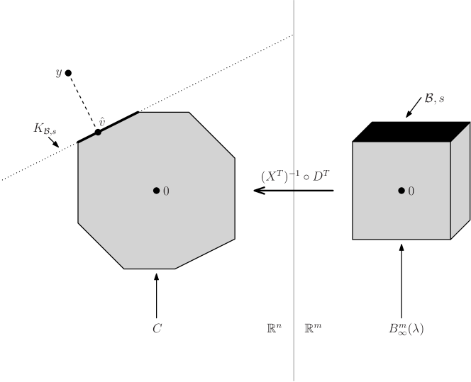
Figure 1: Geometry of the generalized lasso dual problem (4). As in (6), the dual solution $\hat{v}$ may be seen as the projection of $y$ onto a set $C$, and as in (7), the primal fit $X\hat{\beta}$ may be seen as the residual from this projection. Here, $C=(X^{T})^{-1}(D^{T}B^{m}_{\infty}(\lambda))$, and as $B^{m}_{\infty}(\lambda)$ is a polyhedron (and the image or inverse image of a polyhedron under a linear map is still a polyhedron), $C$ is a polyhedron as well. This can be used to derive the implicit form (8) for $X\hat{\beta}$, based on the face of $C$ on which $\hat{v}$ lies, as explained in Remark 2.

Remark 2.

As an alternative to the derivation based on the KKT conditions described above, the result (8) can be argued directly from the geometry surrounding the dual problem (4). See Figure 1 for an accompanying illustration. Given that $\hat{\gamma}$ has boundary set and signs $\mathcal{B},s$, and $\hat{u}=\lambda\hat{\gamma}$ from (5), we see that $\hat{u}$ must lie on the face of $B^{m}_{\infty}(\lambda)$ whose affine span is $E_{\mathcal{B},s}=\{u\in\mathbb{R}^{m}:u_{\mathcal{B},s}=\lambda s\}$; this face is colored in black on the right-hand side of the figure. Since $X^{T}\hat{v}=D^{T}\hat{u}$, this means that $\hat{v}$ lies on the face of $C$ whose affine span is $K_{\mathcal{B},s}=(X^{T})^{-1}D^{T}E_{\mathcal{B},s}$; this face is colored in black on the left-hand side of the figure, and its affine span $K_{\mathcal{B},s}$ is drawn as a dotted line. Hence, we may refine our view of $\hat{v}$ in (6), and in turn, $X\hat{\beta}$ in (7): namely, we may view $\hat{v}$ as the projection of $y$ onto the affine space $K_{\mathcal{B},s}$ (instead of $C$), and the fit $X\hat{\beta}$ as the residual from this affine projection. A straightforward calculation shows that $K_{\mathcal{B},s}=\lambda(P_{\mathrm{null}(D_{-\mathcal{B}})}X^{T})^{+}D_{\mathcal{B}}^{T}s+\mathrm{null}(P_{\mathrm{null}(D_{-\mathcal{B}})}X^{T})$, and another straightforward calculation shows that the residual from projecting $y$ onto $K_{\mathcal{B},s}$ is (8).

From the expression in (8) for the fit $X\hat{\beta}$, we also see that the solution $\hat{\beta}$ corresponding to the optimal subgradient $\hat{\gamma}$ and its boundary set and signs $\mathcal{B},s$ must take the form

$$\hat{\beta}=(XP_{\mathrm{null}(D_{-\mathcal{B}})})^{+}\big{(}y-\lambda(P_{\mathrm{null}(D_{-\mathcal{B}})}X^{T})^{+}D_{\mathcal{B}}^{T}s\big{)}+b,$$ (9)

for some $b\in\mathrm{null}(XP_{\mathrm{null}(D_{-\mathcal{B}})})$. Combining this with $b\in\mathrm{null}(D_{-\mathcal{B}})$ (following from $D_{-\mathcal{B}}\hat{\beta}=0$), we moreover have that $b\in\mathrm{null}(X)\cap\mathrm{null}(D_{-\mathcal{B}})$. In fact, any such point $b\in\mathrm{null}(X)\cap\mathrm{null}(D_{-\mathcal{B}})$ yields a generalized lasso solution $\hat{\beta}$ in (9) provided that

$$s_{i}\cdot D_{i}\Big{[}(XP_{\mathrm{null}(D_{-\mathcal{B}})})^{+}\big{(}y-\lambda(P_{\mathrm{null}(D_{-\mathcal{B}})}X^{T})^{+}D_{\mathcal{B}}^{T}s\big{)}+b\Big{]}\geq 0,\quad\text{for $i\in\mathcal{B}$},$$

which says that $\hat{\gamma}$ appropriately matches the signs of the nonzero components of $D\hat{\beta}$, thus $\hat{\gamma}$ remains a proper subgradient.

We can now begin to inspect conditions for uniqueness of the generalized lasso solution. For a given boundary set $\mathcal{B}$ of an optimal subgradient $\hat{\gamma}$, if we know that $\mathrm{null}(X)\cap\mathrm{null}(D_{-\mathcal{B}})=\{0\}$, then there can only be one solution $\hat{\beta}$ corresponding to $\hat{\gamma}$ (i.e., such that $(\hat{\beta},\hat{\gamma})$ jointly satisfy (2), (3)), and it is given by the expression in (9) with $b=0$. Further, if we know that $\mathrm{null}(X)\cap\mathrm{null}(D_{-\mathcal{B}})=\{0\}$ for all boundary sets $\mathcal{B}$ of optimal subgradients, and the space $\mathrm{null}(D_{-\mathcal{B}})$ is invariant over all choices of boundary sets $\mathcal{B}$ of optimal subgradients, then the right-hand side in (9) with $b=0$ must agree for all proper instantiations of $\mathcal{B},s$ and it gives the unique generalized lasso solution. We elaborate on this in the next section.

2.3 Invariance of the linear space $X\mathrm{null}(D_{-\mathcal{B}})$

Before diving into the technical details on conditions for uniqueness in the next section, we recall a key result from Tibshirani and Taylor (2012).

Lemma 3 (Lemma 10 in Tibshirani and Taylor, 2012).

Fix any $X,D$, and $\lambda>0$. There is a set $\mathcal{N}\subseteq\mathbb{R}^{n}$ of Lebesgue measure zero (that depends on $X,D,\lambda$), such that for $y\notin\mathcal{N}$, all boundary sets $\mathcal{B}$ associated with optimal subgradients in the generalized lasso problem (1) give rise to the same subspace $X\mathrm{null}(D_{-\mathcal{B}})$, i.e., there is a single linear subspace $L\subseteq\mathbb{R}^{n}$ such that $L=X\mathrm{null}(D_{-\mathcal{B}})$ for all boundary sets $\mathcal{B}$ of optimal subgradients. Moreover, for $y\notin\mathcal{N}$, $L=X\mathrm{null}(D_{-\mathcal{A}})$ for all active sets $\mathcal{A}$ associated with generalized lasso solutions.

3 Sufficient conditions for uniqueness

3.1 A condition on certain linear independencies

We start by formalizing the discussion on uniqueness in the paragraphs proceeding (9). As before, let $\lambda>0$, and let $\mathcal{B}$ denote the boundary set associated with an optimal subgradient in (1). Denote by $U(\mathcal{B})\in\mathbb{R}^{p\times k(\mathcal{B})}$ a matrix with linearly independent columns that span $\mathrm{null}(D_{-\mathcal{B}})$. It is not hard to see that

$$\mathrm{null}(X)\cap\mathrm{null}(D_{-\mathcal{B}})=\{0\}\iff\mathrm{null}\big{(}XU(\mathcal{B})\big{)}=\{0\}\iff\mathrm{rank}\big{(}XU(\mathcal{B})\big{)}=k(\mathcal{B}).$$

Let us assign now such a basis matrix $U(\mathcal{B})\in\mathbb{R}^{p\times k(\mathcal{B})}$ to each boundary set $\mathcal{B}$ corresponding to an optimal subgradient in (1). We claim that there is a unique generalized lasso solution, as given in (9) with $b=0$, provided that the following two conditions holds:

$$\mathrm{rank}\big{(}XU(\mathcal{B})\big{)}=k(\mathcal{B})\text{ for all boundary sets $\mathcal{B}$ associated with optimal subgradients, and}$$ (10)

$$\mathrm{null}(D_{-\mathcal{B}})\text{ is invariant across all boundary sets $\mathcal{B}$ associated with optimal subgradients}.$$ (11)

To see this, note that if the space $\mathrm{null}(D_{-\mathcal{B}})$ is invariant across all achieved boundary sets $\mathcal{B}$ then so is the matrix $P_{\mathrm{null}(D_{-\mathcal{B}})}$. This, and the fact that $P_{\mathrm{null}(D_{-\mathcal{B}})}D_{B}^{T}s=P_{\mathrm{null}(D_{-\mathcal{B}})}D^{T}\hat{\gamma}$ where $D^{T}\hat{\gamma}$ is unique from Lemma 2, ensures that the right-hand side in (9) with $b=0$ agrees no matter the choice of boundary set and signs $\mathcal{B},s$.

Remark 3.

For any subset $\mathcal{B}\subseteq\{1,\ldots,m\}$, and any matrices $U(\mathcal{B}),\tilde{U}(\mathcal{B})\in\mathbb{R}^{p\times k(\mathcal{B})}$ whose columns form a basis for $\mathrm{null}(D_{-\mathcal{B}})$, it is easy to check that $\mathrm{rank}(XU(\mathcal{B}))=k(\mathcal{B})\iff\mathrm{rank}(X\tilde{U}(\mathcal{B}))=k(\mathcal{B})$. Therefore condition (10) is well-defined, i.e., it does not depend on the choice of basis matrix $U(\mathcal{B})$ associated with $\mathrm{null}(D_{-\mathcal{B}})$ for each boundary set $\mathcal{B}$.

We now show that, thanks to Lemma 3, condition (10) (almost everywhere) implies (11), so the former is alone sufficient for uniqueness.

Lemma 4.

Fix any $X,D$, and $\lambda>0$. For $y\notin\mathcal{N}$, where $\mathcal{N}\subseteq\mathbb{R}^{n}$ has Lebesgue measure zero as in Lemma 3, condition (10) implies (11). Hence, for almost every $y$, condition (10) is itself sufficient to imply uniqueness of the generalized lasso solution.

Proof.

Let $y\notin\mathcal{N}$, and let $L$ be the linear subspace from Lemma 3, i.e., $L=X\mathrm{null}(D_{-\mathcal{B}})$ for any boundary set $\mathcal{B}$ associated with an optimal subgradient in the generalized lasso problem at $y$. Now fix a particular boundary set $\mathcal{B}$ associated with an optimal subgradient and define the linear map $\mathcal{X}:\mathrm{null}(D_{-\mathcal{B}})\to L$ by $\mathcal{X}(u)=Xu$. By construction, this map is surjective. Moreover, assuming (10), it is injective, as

$$XU(\mathcal{B})a=XU(\mathcal{B})b\iff XU(\mathcal{B})(a-b)=0,$$

and the right-hand side cannot be true unless $a=b$. Therefore, $\mathcal{X}$ is bijective and has a linear inverse, and we may write $\mathrm{null}(D_{-\mathcal{B}})=\mathcal{X}^{-1}(L)$. As $\mathcal{B}$ was arbitrary, this shows the invariance of $\mathrm{null}(D_{-\mathcal{B}})$ over all proper choices of $\mathcal{B}$, whenever $y\notin\mathcal{N}$. ∎

From Lemma 4, we see that an (almost everywhere) sufficient condition for a unique solution in (1) is that the vectors $XU_{i}(\mathcal{B})\in\mathbb{R}^{n}$, $i=1,\ldots,k(\mathcal{B})$ are linearly independent, for all instantiations of boundary sets $\mathcal{B}$ of optimal subgradients. This may seem a little circular, to give a condition for uniqueness that itself is expressed in terms of the subgradients of solutions. But we will not stop at (10), and will derive more explicit conditions on $y,X,D$, and $\lambda>0$ that imply (10) and therefore uniqueness of the solution in (1).

3.2 A refined condition on linear independencies

The next lemma shows that when condition (10) fails, there is a specific type of linear dependence among the columns of $XU(\mathcal{B})$, for a boundary set $\mathcal{B}$. The proof is not difficult, but involves careful manipulations of the KKT conditions (2), and we defer it until the appendix.

Lemma 5.

Fix any $X,D$, and $\lambda>0$. Let $y\notin\mathcal{N}$, the set of zero Lebesgue measure as in Lemma 3. Assume that $\mathrm{null}(X)\cap\mathrm{null}(D)=\{0\}$, and that the generalized lasso solution is not unique. Then there is a pair of boundary set and signs $\mathcal{B},s$ corresponding to an optimal subgradient in problem (1), such that for any matrix $U(\mathcal{B})\in\mathbb{R}^{p\times k(\mathcal{B})}$ whose columns form a basis for $\mathrm{null}(D_{-\mathcal{B}})$, the following property holds of $Z=XU(\mathcal{B})$ and $\tilde{s}=U(\mathcal{B})^{T}D_{\mathcal{B}}^{T}s$: there exist indices $i_{1},\ldots,i_{k}\in\{1,\ldots,k(\mathcal{B})\}$ with $k\leq n+1$ and $\tilde{s}_{i_{1}}\neq 0$, such that

$$Z_{i_{2}}\in\mathrm{span}(\{Z_{i_{3}},\ldots,Z_{i_{k}}\}),$$ (12)

when $\tilde{s}_{i_{2}}=\cdots=\tilde{s}_{i_{k}}=0$, and

$$Z_{i_{1}}/\tilde{s}_{i_{1}}\in\mathrm{aff}(\{Z_{i_{j}}/\tilde{s}_{i_{j}}:\tilde{s}_{i_{j}}\neq 0,\,j\geq 2\})+\mathrm{span}(\{Z_{i_{j}}:\tilde{s}_{i_{j}}=0\}),$$ (13)

when at least one of $\tilde{s}_{i_{2}},\ldots,\tilde{s}_{i_{k}}$ is nonzero.

The spaces on the right-hand sides of both (12), (13) are of dimension at most $n-1$. To see this, note that $\mathrm{dim}(\mathrm{span}(\{Z_{i_{3}},\ldots,Z_{i_{k}}\}))\leq k-2\leq n-1$, and also

$$\mathrm{dim}\big{(}\mathrm{aff}(\{Z_{i_{j}}/\tilde{s}_{i_{j}}:\tilde{s}_{i_{j}}\neq 0,\,j\geq 2\})\big{)}+\mathrm{dim}\big{(}\mathrm{span}(\{Z_{i_{j}}:\tilde{s}_{i_{j}}=0\})\big{)}\leq|\mathcal{J}|-2+|\mathcal{J}^{c}|=k-2\leq n-1,$$

where $\mathcal{J}=\{j\in\{1,\ldots,k\}:\tilde{s}_{i_{j}}\neq 0\}$. Hence, because these spaces are at most $(n-1)$-dimensional, neither condition (12) nor (13) should be “likely” under a continuous distribution for the predictor variables $X$. This is made precise in the next subsection.

Before this, we define a deterministic condition on $X$ that ensures special linear dependencies between the (transformed) columns, as in (12), (13), never hold.

Definition 1.

Fix $D\in\mathbb{R}^{m\times p}$. We say that a matrix $X\in\mathbb{R}^{n\times p}$ is in $D$-general position (or $D$-GP) if the following property holds. For each subset $\mathcal{B}\subseteq\{1,\ldots,m\}$ and sign vector $s\in\{-1,1\}^{|\mathcal{B}|}$, there is a matrix $U(\mathcal{B})\in\mathbb{R}^{p\times k(\mathcal{B})}$ whose columns form a basis for $\mathrm{null}(D_{-\mathcal{B}})$, such that for $Z=XU(\mathcal{B})$, $\tilde{s}=U(\mathcal{B})^{T}D_{\mathcal{B}}^{T}s$, and all $i_{1},\ldots,i_{k}\in\{1,\ldots,k(\mathcal{B})\}$ with $\tilde{s}_{i_{1}}\neq 0$ and $k\leq n+1$, it holds that

1. $Z_{i_{2}}\notin\mathrm{span}(\{Z_{i_{3}},\ldots,Z_{i_{k}}\})$, when $\tilde{s}_{i_{2}}=\cdots=\tilde{s}_{i_{k}}=0$;

2. $Z_{i_{1}}/\tilde{s}_{i_{1}}\notin\mathrm{aff}(\{Z_{i_{j}}/\tilde{s}_{i_{j}}:\tilde{s}_{i_{j}}\neq 0,\,j\geq 2\})+\mathrm{span}(\{Z_{i_{j}}:\tilde{s}_{i_{j}}=0\})$, when at least one of $\tilde{s}_{i_{2}},\ldots,\tilde{s}_{i_{k}}$ is nonzero.

Remark 4.

Though the definition may appear somewhat complicated, a matrix $X$ being in $D$-GP is actually quite a weak condition, and can hold regardless of the (relative) sizes of $n,p$. We will show in the next subsection that it holds almost surely under an arbitrary continuous probability distribution for the entries of $X$. Further, when $X=I$, the above definition essentially reduces to the usual notion of general position (refer to, e.g., Tibshirani, 2013 for this definition).

When $X$ is in $D$-GP, we have (by definition) that (12), (13) cannot hold for any $\mathcal{B}\subseteq\{1,\ldots,m\}$ and $s\in\{-1,1\}^{|\mathcal{B}|}$ (not just boundary sets and signs); therefore, by the contrapositive of Lemma 5, if we additionally have $y\notin\mathcal{N}$ and $\mathrm{null}(X)\cap\mathrm{null}(D)=\{0\}$, then the generalized lasso solution must be unique. To emphasize this, we state it as a lemma.

Lemma 6.

Fix any $X,D$, and $\lambda>0$. If $y\notin\mathcal{N}$, the set of zero Lebesgue measure as in Lemma 3, $\mathrm{null}(X)\cap\mathrm{null}(D)=\{0\}$, and $X$ is in $D$-GP, then the generalized lasso solution is unique.

3.3 Absolutely continuous predictor variables

We give an important result that shows the $D$-GP condition is met almost surely for continuously distributed predictors. There are no restrictions on the relative sizes of $n,p$. The proof of the next result uses elementary probability arguments and is deferred until the appendix.

Lemma 7.

Fix $D\in\mathbb{R}^{m\times p}$, and assume that the entries of $X\in\mathbb{R}^{n\times p}$ are drawn from a distribution that is absolutely continuous with respect to $(np)$-dimensional Lebesgue measure. Then $X$ is in $D$-GP almost surely.

We now present a result showing that the base condition $\mathrm{null}(X)\cap\mathrm{null}(D)=\{0\}$ is met almost surely for continuously distributed predictors, provided that $p\leq n$, or $p>n$ and the null space of $D$ is not too large. Its proof is elementary and found in the appendix.

Lemma 8.

Fix $D\in\mathbb{R}^{m\times p}$, and assume that the entries of $X\in\mathbb{R}^{n\times p}$ are drawn from a distribution that is absolutely continuous with respect to $(np)$-dimensional Lebesgue measure. If either $p\leq n$, or $p>n$ and $\mathrm{nullity}(D)\leq n$, then $\mathrm{null}(X)\cap\mathrm{null}(D)=\{0\}$ almost surely.

Putting together Lemmas 6, 7, 8 gives our main result on the uniqueness of the generalized lasso solution.

Theorem 1.

Fix any $D$ and $\lambda>0$. Assume the joint distribution of $(X,y)$ is absolutely continuous with respect to $(np+n)$-dimensional Lebesgue measure. If $p\leq n$, or else $p>n$ and $\mathrm{nullity}(D)\leq n$, then the solution in the generalized lasso problem (1) is unique almost surely.

Remark 5.

If $D$ has full row rank, then by Lemma 2 the optimal subgradient $\hat{\gamma}$ is unique and so the boundary set $\mathcal{B}$ is also unique. In this case, condition (11) is vacuous and condition (10) is sufficient for uniqueness of the generalized lasso solution for every $y$ (i.e., we do not need to rely on Lemma 4, which in turn uses Lemma 3, to prove that (10) is sufficient for almost every $y$). Hence, in this case, the condition in Theorem 1 that $y|X$ has an absolutely continuous distribution is not needed, and (with the other conditions in place) uniqueness holds for every $y$, almost surely over $X$. Under this (slight) sharpening, Theorem 1 with $D=I$ reduces to the result in Lemma 4 of Tibshirani (2013).

Remark 6.

Generally speaking, the condition that $\mathrm{nullity}(D)\leq n$ in Theorem 1 (assumed in the case $p>n$) is not strong. In many applications of the generalized lasso, the dimension of the null space of $D$ is small and fixed (i.e., it does not grow with $n$). For example, recall Corollary 1, where the lower bound $n$ in each of the cases reflects the dimension of the null space.

3.4 Standardized predictor variables

A common preprocessing step, in many applications of penalized modeling such as the generalized lasso, is to standardize the predictors $X\in\mathbb{R}^{n\times p}$, meaning, center each column to have mean 0, and then scale each column to have norm 1. Here we show that our main uniqueness results carry over, mutatis mutandis, to the case of standardized predictor variables. All proofs in this subsection are deferred until the appendix.

We begin by studying the case of centering alone. Let $M=I-\mathds{1}\mathds{1}^{T}/n\in\mathbb{R}^{n\times n}$ be the centering map, and consider the centered generalized lasso problem

$$\mathop{\mathrm{minimize}}_{\beta\in\mathbb{R}^{p}}\;\frac{1}{2}\|y-MX\beta\|_{2}^{2}+\lambda\|D\beta\|_{1}.$$ (14)

We have the following uniqueness result for centered predictors.

Corollary 2.

Fix any $D$ and $\lambda>0$. Assume the distribution of $(X,y)$ is absolutely continuous with respect to $(np+n)$-dimensional Lebesgue measure. If $p\leq n-1$, or $p>n-1$ and $\mathrm{nullity}(D)\leq n-1$, then the solution in the centered generalized lasso problem (14) is unique almost surely.

Remark 7.

The exact same result as stated in Corollary 2 holds for the generalized lasso problem with intercept

$$\mathop{\mathrm{minimize}}_{\beta_{0}\in\mathbb{R},\,\beta\in\mathbb{R}^{p}}\;\frac{1}{2}\|y-\beta_{0}\mathds{1}-X\beta\|_{2}^{2}+\lambda\|D\beta\|_{1}.$$ (15)

This is because, by minimizing over $\beta_{0}$ in problem (15), we find that this problem is equivalent to minimization of

$$\frac{1}{2}\|My-MX\beta\|_{2}^{2}+\lambda\|D\beta\|_{1}$$

over $\beta$, which is just a generalized lasso problem with response $V_{-1}^{T}y$ and predictors $V_{-1}^{T}X$, where the notation here is as in the proof of Corollary 2.

Next we treat the case of scaling alone. Let $W_{X}=\mathrm{diag}(\|X_{1}\|_{2},\ldots,\|X_{p}\|_{2})\in\mathbb{R}^{p\times p}$, and consider the scaled generalized lasso problem

$$\mathop{\mathrm{minimize}}_{\beta\in\mathbb{R}^{p}}\;\frac{1}{2}\|y-XW_{X}^{-1}\beta\|_{2}^{2}+\lambda\|D\beta\|_{1}.$$ (16)

We give a helper lemma, on the distribution of a continuous random vector, post scaling.

Lemma 9.

Let $Z\in\mathbb{R}^{n}$ be a random vector whose distribution is absolutely continuous with respect to $n$-dimensional Lebesgue measure. Then, the distribution of $Z/\|Z\|_{2}$ is absolutely continuous with respect to $(n-1)$-dimensional Hausdorff measure restricted to the $(n-1)$-dimensional unit sphere, $\mathbb{S}^{n-1}=\{x\in\mathbb{R}^{n}:\|x\|_{2}=1\}$.

We give a second helper lemma, on the $(n-1)$-dimensional Hausdorff measure of an affine space intersected with the unit sphere $\mathbb{S}^{n-1}$ (which is important for checking that the scaled predictor matrix is in $D$-GP, because here we must check that none of its columns lie in a finite union of affine spaces).

Lemma 10.

Let $A\subseteq\mathbb{R}^{n}$ be an arbitrary affine space, with $\mathrm{dim}(A)\leq n-1$. Then $\mathbb{S}^{n-1}\cap A$ has $(n-1)$-dimensional Hausdorff measure zero.

We present a third helper lemma, which establishes that for absolutely continuous $X$, the scaled predictor matrix $XW_{X}^{-1}$ is in $D$-GP and satisfies the appropriate null space condition, almost surely.

Lemma 11.

Fix $D\in\mathbb{R}^{m\times p}$, and assume that $X\in\mathbb{R}^{n\times p}$ has entries drawn from a distribution that is absolutely continuous with respect to $(np)$-dimensional Lebesgue measure. Then $XW_{X}^{-1}$ is in $D$-GP almost surely. Moreover, if $p\leq n$, or $p>n$ and $\mathrm{nullity}(D)\leq n$, then $\mathrm{null}(XW_{X}^{-1})\cap\mathrm{null}(D)=\{0\}$ almost surely.

Combining Lemmas 6, 11 gives the following uniqueness result for scaled predictors.

Corollary 3.

Fix any $D$ and $\lambda>0$. Assume the distribution of $(X,y)$ is absolutely continuous with respect to $(np+n)$-dimensional Lebesgue measure. If $p\leq n$, or else $p>n$ and $\mathrm{nullity}(D)\leq n$, then the solution in the scaled generalized lasso problem (16) is unique almost surely.

Finally, we consider the standardized generalized lasso problem,

$$\mathop{\mathrm{minimize}}_{\beta\in\mathbb{R}^{p}}\;\frac{1}{2}\|y-MXW_{MX}^{-1}\beta\|_{2}^{2}+\lambda\|D\beta\|_{1},$$ (17)

where, note, the predictor matrix $MXW_{MX}^{-1}$ has standardized columns, i.e., each column has been centered to have mean 0, then scaled to have norm 1. We have the following uniqueness result.

Corollary 4.

Fix any $D$ and $\lambda>0$. Assume the distribution of $(X,y)$ is absolutely continuous with respect to $(np+n)$-dimensional Lebesgue measure. If $p\leq n-1$, or $p>n-1$ and $\mathrm{nullity}(D)\leq n-1$, then the solution in the standardized generalized lasso problem (17) is unique almost surely.

4 Smooth, strictly convex loss functions

4.1 Generalized lasso with a general loss

We now extend some of the preceding results beyond the case of squared error loss, as considered previously. In particular, we consider the problem

$$\mathop{\mathrm{minimize}}_{\beta\in\mathbb{R}^{p}}\;G(X\beta;y)+\lambda\|D\beta\|_{1},$$ (18)

where we assume, for each $y\in\mathbb{R}^{n}$, that the function $G(\,\cdot\,;y)$ is essentially smooth and essentially strictly convex on $\mathbb{R}^{n}$. These two conditions together mean that $G(\,\cdot\,;y)$ is a closed proper convex function, differentiable and strictly convex on the interior of its domain (assumed to be nonempty), with the norm of its gradient approaching $\infty$ along any sequence approaching the boundary of its domain. A function that is essentially smooth and essentially strictly convex is also called, according to some authors, of Legendre type; see Chapter 26 of Rockafellar (1970). An important special case of a Legendre function is one that is differentiable and strictly convex, with full domain (all of $\mathbb{R}^{n}$).

For much of what follows, we will focus on loss functions of the form

$$G(z;y)=-y^{T}z+\psi(z),$$ (19)

for an essentially smooth and essentially strictly convex function $\psi$ on $\mathbb{R}^{n}$ (not depending on $y$). This is a weak restriction on $G$ and encompasses, e.g., the cases in which $G$ is the negative log-likelihood function from a generalized linear model (GLM) for the entries of $y|X$ with a canonical link function, where $\psi$ is the cumulant generating function. In the case of, say, Bernoulli or Poisson models, this is

$$G(z;y)=-y^{T}z+\sum_{i=1}^{n}\log(1+e^{z_{i}}),\quad\text{or}\quad G(z;y)=-y^{T}z+\sum_{i=1}^{n}e^{z_{i}},$$

respectively. For brevity, we will often write the loss function as $G(X\beta)$, hiding the dependence on the response vector $y$.

4.2 Basic facts, KKT conditions, and the dual

The next lemma follows from arguments identical to those for Lemma 1.

Lemma 12.

For any $y,X,D,\lambda\geq 0$, and for $G$ essentially smooth and essentially strictly convex, the following holds of problem (18).

1. There is either zero, one, or uncountably many solutions.

2. Every solution $\hat{\beta}$ gives rise to the same fitted value $X\hat{\beta}$.

3. If $\lambda>0$, then every solution $\hat{\beta}$ gives rise to the same penalty value $\|D\hat{\beta}\|_{1}$.

Note the difference between Lemmas 12 and 1, part (i): for an arbitrary (essentially smooth and essentially strictly convex) $G$, the criterion in (18) need not attain its infimum, whereas the criterion in (1) always does. This happens because the criterion in (18) can have directions of strict recession (i.e., directions of recession in which the criterion is not constant), whereas the citerion in (1) cannot. Thus in general, problem (18) need not have a solution; this is true even in the most fundamental cases of interest beyond squared loss, e.g., the case of a Bernoulli negative log-likelihood $G$. Later in Lemma 14, we give a sufficient condition for the existence of solutions in (18).

The KKT conditions for problem (18) are

$$-X^{T}\nabla G(X\hat{\beta})=\lambda D^{T}\hat{\gamma},$$ (20)

where $\hat{\gamma}\in\mathbb{R}^{m}$ is (as before) a subgradient of the $\ell_{1}$ norm evaluated at $D\hat{\beta}$,

$$\hat{\gamma}_{i}\in\begin{cases}\{\mathrm{sign}((D\hat{\beta})_{i})\}&\text{if $(D\hat{\beta})_{i}\neq 0$}\\ [-1,1]&\text{if $(D\hat{\beta})_{i}=0$}\end{cases},\quad\text{for $i=1,\ldots,m$}.$$ (21)

As in the squared loss case, uniqueness of $X\hat{\beta}$ by Lemma 12, along with (20), imply the next result.

Lemma 13.

For any $y,X,D,\lambda>0$, and $G$ essentially smooth and essentially strictly convex, every optimal subgradient $\hat{\gamma}$ in problem (18) gives rise to the same value of $D^{T}\hat{\gamma}$. Furthermore, when $D$ has full row rank, the optimal subgradient $\hat{\gamma}$ is unique, assuming that problem (18) has a solution in the first place.

Denote by $G^{*}$ the conjugate function of $G$. When $G$ is essentially smooth and essentially strictly convex, the following facts hold (e.g., see Theorem 26.5 of Rockafellar (1970)):

• its conjugate $G^{*}$ is also essentially smooth and essentially strictly convex; and

• the map $\nabla G:\mathrm{int}(\mathrm{dom}(G))\to\mathrm{int}(\mathrm{dom}(G^{*}))$ is a homeomorphism with inverse $(\nabla G)^{-1}=\nabla G^{*}$.

The conjugate function is intrinsically tied to duality, directions of recession, and the existence of solutions. Standard arguments in convex analysis, deferred to the appendix, give the next result.

Lemma 14.

Fix any $y,X,D$, and $\lambda\geq 0$. Assume $G$ is essentially smooth and essentially strictly convex. The Lagrangian dual of problem (18) can be written as

$$\mathop{\mathrm{minimize}}_{u\in\mathbb{R}^{m},\,v\in\mathbb{R}^{u}}\;G^{*}(-v)\quad\mathop{\mathrm{subject\,\,to}}\quad X^{T}v=D^{T}u,\;\|u\|_{\infty}\leq\lambda,$$ (22)

where $G^{*}$ is the conjugate of $G$. Any dual optimal pair $(\hat{u},\hat{v})$ in (22), and primal optimal solution-subgradient pair $(\hat{\beta},\hat{\gamma})$ in (18), i.e., satisfying (20), (21), assuming they all exist, must satisfy the primal-dual relationships

$$\nabla G(X\hat{\beta})=-\hat{v},\quad\text{and}\quad\hat{u}=\lambda\hat{\gamma}.$$ (23)

Lastly, existence of primal and dual solutions is guaranteed under the conditions

$$0\in\mathrm{int}(\mathrm{dom}(G)),$$ (24)

$$(-C)\cap\mathrm{int}(\mathrm{ran}(\nabla G))\neq\emptyset,$$ (25)

where $C=(X^{T})^{-1}(D^{T}B^{m}_{\infty}(\lambda))$. In particular, under (24) and $C\neq\emptyset$, a solution exists in the dual problem (22), and under (24), (25), a solution exists in the primal problem (18).

Assuming that primal and dual solutions exist, we see from (23) in the above lemma that $\hat{v}$ must be unique (by uniqueness of $X\hat{\beta}$, from Lemma 12), but $\hat{u}$ need not be (as $\hat{\gamma}$ is not necessarily unique). Moreover, under condition (24), we know that $G$ is differentiable at 0, and $\nabla G^{*}(\nabla G(0))=0$, hence we may rewrite (22) as

$$\mathop{\mathrm{minimize}}_{u\in\mathbb{R}^{m},\,v\in\mathbb{R}^{n}}\;D_{G^{*}}\big{(}-v,\nabla G(0)\big{)}\quad\mathop{\mathrm{subject\,\,to}}\quad X^{T}v=D^{T}u,\;\|u\|_{\infty}\leq\lambda,$$ (26)

where $D_{f}(x,z)=f(x)-f(z)-\langle\nabla f(z),x-z\rangle$ denotes the Bregman divergence between points $x,z$, with respect to a function $f$. Optimality of $\hat{v}$ in (26) may be expressed as

$$\hat{v}=-P^{G^{*}}_{-C}\big{(}\nabla G(0)\big{)},\quad\text{where}\;\,C=(X^{T})^{-1}\big{(}D^{T}B^{m}_{\infty}(\lambda)\big{)}.$$ (27)

Here, recall $(X^{T})^{-1}(S)$ denotes the preimage of a set $S$ under the linear map $X^{T}$, $D^{T}S$ denotes the image of a set $S$ under the linear map $D^{T}$, $B^{m}_{\infty}(\lambda)=\{u\in\mathbb{R}^{m}:\|u\|_{\infty}\leq\lambda\}$ is the $\ell_{\infty}$ ball of radius $\lambda$ in $\mathbb{R}^{m}$, and now $P^{f}_{S}(\cdot)$ is the projection operator onto a set $S$ with respect to the Bregman divergence of a function $f$, i.e., $P^{f}_{S}(z)=\mathop{\mathrm{arg\,min}}_{x\in S}D_{f}(x,z)$. From (27) and (23), we see that

$$X\hat{\beta}=\nabla G^{*}\Big{(}P^{G^{*}}_{-C}\big{(}\nabla G(0)\big{)}\Big{)}.$$ (28)

We note the analogy between (27), (28) and (6), (7) in the squared loss case; for $G(z)=\frac{1}{2}\|y-z\|_{2}^{2}$, we have $\nabla G(0)=-y$, $G^{*}(z)=\frac{1}{2}\|y+z\|_{2}^{2}-\frac{1}{2}\|y\|_{2}^{2}$, $\nabla G^{*}(z)=y+z$, $-P^{G^{*}}_{-C}(\nabla G(0))=P_{C}(y)$, and so (27), (28) match (6), (7), respectively. But when $G$ is non-quadratic, we see that the dual solution $\hat{v}$ and primal fit $X\hat{\beta}$ are given in terms of a non-Euclidean projection operator, defined with respect to the Bregman divergence of $G^{*}$. See Figure 2 for an illustration. This complicates the study of the primal and dual problems, in comparison to the squared loss case; still, as we will show in the coming subsections, several key properties of primal and dual solutions carry over to the current general loss setting.

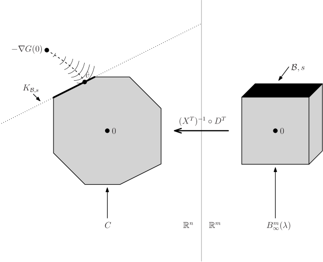
Figure 2: Geometry of the dual problem (26), for a general loss $G$. As in (27), the dual solution $\hat{v}$ may be seen as the Bregman projection of $-\nabla G(0)$ onto a set $C$ with respect to the map $x\mapsto G^{*}(-x)$ (where $G^{*}$ is the conjugate of $G$). Shown in the figure are the contours of this map, around $-\nabla G(0)$; the point $\hat{v}$ lies at the intersection of the lowest-level contour and $C$. Here, as in the squared loss case, $C=(X^{T})^{-1}(D^{T}B^{m}_{\infty}(\lambda))$, which is a polyhedron. This realization can be used to derive the implicit form (38) for $X\hat{\beta}$, based on (28) and the face of $C$ on which $\hat{v}$ lies, as explained in Remark 10.

4.3 Existence in (regularized) GLMs

Henceforth, we focus on the case in which $G$ takes the form (19). The stationarity condition (20) is

$$X^{T}\big{(}y-\nabla\psi(X\hat{\beta})\big{)}=\lambda D^{T}\hat{\gamma},$$ (29)

and using the identities $G^{*}(x)=\psi^{*}(x+y)$, $P^{G^{*}}_{S}(x)=P^{\psi^{*}}_{S+y}(x+y)-y$, the dual and primal projections, (27) and (28), become

$$\hat{v}=y-P^{\psi^{*}}_{y-C}\big{(}\nabla\psi(0)\big{)},\quad\text{and}\quad X\hat{\beta}=\nabla\psi^{*}\Big{(}P^{\psi^{*}}_{y-C}\big{(}\nabla\psi(0)\big{)}\Big{)}.$$ (30)

As a check, in the squared loss case, we have $\psi(z)=\frac{1}{2}\|z\|_{2}^{2}$, $\nabla\psi(0)=0$, $\psi^{*}(z)=\frac{1}{2}\|z\|_{2}^{2}$, $\nabla\psi^{*}(z)=z$, $P^{\psi^{*}}_{y-C}(\nabla\psi(0))=y-P_{C}(y)$, so (30) matches (6), (7). Finally, the conditions (24), (25) that guarantee the existence of primal and dual solutions become

$$0\in\mathrm{int}(\mathrm{dom}(\psi)),$$ (31)

$$y\in\mathrm{int}(\mathrm{ran}(\nabla\psi))+C,$$ (32)

where recall $C=(X^{T})^{-1}(D^{T}B^{m}_{\infty}(\lambda))$.

We take somewhat of a detour from our main goal (establishing uniqueness in (18)), and study the existence conditions (31), (32). To gather insight, we examine them in detail for some cases of interest. We begin by looking at unregularized ($\lambda=0$) logistic and Poisson regression. The proof of the next result is straightforward in all but the logistic regression case, and is given in the appendix.

Lemma 15.

Fix any $y,X$. Assume that $G$ is of the form (19), where $\psi$ is essentially smooth and essentially strictly convex, satisfying $0\in\mathrm{int}(\mathrm{dom}(\psi))$. Consider problem (18), with $\lambda=0$. Then the sufficient condition (32) for the existence of a solution is equivalent to

$$y\in\mathrm{int}(\mathrm{ran}(\nabla\psi))+\mathrm{null}(X^{T}).$$ (33)

For logistic regression, where $\psi(z)=\sum_{i=1}^{n}\log(1+e^{z_{i}})$ and $y\in\{0,1\}^{n}$, if we write $Y_{i}=2y_{i}-1\in\{-1,1\}$, $i=1,\ldots,n$, and we denote by $x_{i}\in\mathbb{R}^{p}$, $i=1,\ldots,n$ the rows of $X$, then condition (33) is equivalent to

$$\text{there does not exist $b\neq 0$ such that $Y_{i}x_{i}^{T}b\geq 0$, $i=1,\ldots,n$}.$$ (34)

For Poisson regression, where $\psi(z)=\sum_{i=1}^{n}e^{z_{i}}$ and $y\in\mathbb{N}^{n}$ (where $\mathbb{N}=\{0,1,2,\ldots\}$ denotes the set of natural numbers), condition (33) is equivalent to

$$\text{there exists $\delta\in\mathrm{null}(X^{T})$ such that $y_{i}+\delta_{i}>0$, $i=1,\ldots,n$}.$$ (35)

Remark 8.

For the cases of logistic and Poisson regression, the lemma shows that the sufficient condition (32) for the existence of a solution (note (31) is automatically satisfied, as $\mathrm{dom}(\psi)=\mathbb{R}^{n}$ in these cases) reduces to (34) and (35), respectively. Interestingly, in both cases, this recreates a well-known necessary and sufficient condition for the existence of the maximum likelihood estimate (MLE); see Albert and Anderson (1984) for the logistic regression condition (34), and Haberman (1974) for the Poisson regression condition (35). The former condition (34) is particularly intuitive, and says that the logistic MLE exists if and only if there is no hyperplane that “quasicompletely” separates the points $x_{i}$, $i=1,\ldots,n$ into the positive and negative classes (using the terminology of Albert and Anderson (1984)). For a modern take on this condition, see Candes and Sur (2018).

Now we inspect the regularized case ($\lambda>0$). The proof of the next result is straightforward and can be found in the appendix.

Lemma 16.

Fix any $y,X,D$, and $\lambda>0$. Assume that $G$ is of the form (19), where we are either in the logistic case, $\psi(z)=\sum_{i=1}^{n}\log(1+e^{z_{i}})$ and $y\in\{0,1\}^{n}$, or in the Poisson case, $\psi(z)=\sum_{i=1}^{n}e^{z_{i}}$ and $y\in\mathbb{N}^{n}$ In either case, a sufficient (but not necessary) condition for (32) to hold, and hence for a solution to exist in problem (18), is

$$\mathrm{null}(D)\subseteq\mathrm{null}(X).$$ (36)

Remark 9.

We note that, in particular, condition (36) always holds when $D=I$, which implies that lasso penalized logistic regression and lasso penalized Poisson regression always have solutions.

4.4 Implicit form of solutions

Fix an arbitrary $\lambda>0$, and let $(\hat{\beta},\hat{\gamma})$ denote an optimal solution-subgradient pair, i.e., satisfying (20), (21). As before, we define the boundary set and boundary signs in terms of $\hat{\gamma}$,

$$\mathcal{B}=\big{\{}i\in\{1,\ldots,m\}:|\hat{\gamma}_{i}|=1\big{\}},\quad\text{and}\quad s=\mathrm{sign}(\hat{\gamma}_{\mathcal{B}}).$$

and the active set and active signs in terms of $\hat{\beta}$,

$$\mathcal{A}=\mathrm{supp}(D\hat{\beta})=\big{\{}i\in\{1,\ldots,m\}:(D\hat{\beta})_{i}\neq 0\big{\}},\quad\text{and}\quad r=\mathrm{sign}(\hat{\gamma}_{\mathcal{A}}).$$

By (20), we have that $\mathcal{A}\subseteq\mathcal{B}$. In general, $\mathcal{A},r,\mathcal{B},s$ are not unique, as neither $\hat{\beta}$ nor $\hat{\gamma}$ are.

The next lemma gives an implicit form for the fit and solutions in (18), with $G$ as in (19), akin to the results (8), (9) in the squared loss case. Its proof stems directly from the KKT conditions (29); it is somewhat technical and deferred until the appendix.

Lemma 17.

Fix any $y,X,D$, and $\lambda>0$. Assume that $G$ is of the form (19), where $\psi$ is essentially smooth and essentially strictly convex, and satisfies (31), (32). Let $\hat{\beta}$ be a solution in problem (18), and let $\hat{\gamma}$ be a corresponding optimal subgradient, with boundary set and boundary signs $\mathcal{B},s$. Define the affine subspace

$$K_{\mathcal{B},s}=\lambda(P_{\mathrm{null}(D_{-\mathcal{B}})}X^{T})^{+}D_{\mathcal{B}}^{T}s+\mathrm{null}(P_{\mathrm{null}(D_{-\mathcal{B}})}X^{T}).$$ (37)

Then the unique fit can be expressed as

$$X\hat{\beta}=\nabla\psi^{*}\Big{(}P^{\psi^{*}}_{y-K_{\mathcal{B},s}}\big{(}\nabla\psi(0)\big{)}\Big{)},$$ (38)

and the solution can be expressed as

$$\hat{\beta}=(XP_{\mathrm{null}(D_{-\mathcal{B}})})^{+}\nabla\psi^{*}\Big{(}P^{\psi^{*}}_{y-K_{\mathcal{B},s}}\big{(}\nabla\psi(0)\big{)}\Big{)}+b,$$ (39)

for some $b\in\mathrm{null}(X)\cap\mathrm{null}(D_{-\mathcal{B}})$. Similarly, letting $\mathcal{A},r$ denote the active set and active signs of $\hat{\beta}$, the same expressions hold as in the last two displays with $\mathcal{B},s$ replaced by $\mathcal{A},r$ (i.e., with the affine subspace of interest now being $K_{\mathcal{A},r}=\lambda(P_{\mathrm{null}(D_{-\mathcal{A}})}X^{T})^{+}D_{\mathcal{A}}^{T}r+\mathrm{null}(P_{\mathrm{null}(D_{-\mathcal{A}})}X^{T})$).

Remark 10.

The proof of Lemma 17 derives the representation (38) using technical manipulation of the KKT conditions. But the same result can be derived using the geometry surrounding the dual problem (26). See Figure 2 for an accompanying illustration, and Remark 2 for a similar geometric argument in the squared loss case. As $\hat{\gamma}$ has boundary set and signs $\mathcal{B},s$, and $\hat{u}=\lambda\hat{\gamma}$ from (23), we see that $\hat{u}$ must lie on the face of $B^{m}_{\infty}(\lambda)$ whose affine span is $E_{\mathcal{B},s}=\{u\in\mathbb{R}^{m}:u_{\mathcal{B},s}=\lambda s\}$; and as $X^{T}\hat{v}=D^{T}\hat{u}$, we see that $\hat{v}$ lies on the face of $C$ whose affine span is $K_{\mathcal{B},s}=(X^{T})^{-1}D^{T}E_{\mathcal{B},s}$, which, it can be checked, can be rewritten explicitly as the affine subspace in (37). Hence, the projection of $\nabla G(0)$ onto $-C$ lies on a face whose affine span is $-K_{\mathcal{B},s}$, and we can write

$$-\hat{v}=P^{G^{*}}_{-K_{\mathcal{B},s}}\big{(}\nabla G(0)\big{)},$$

i.e., we can simply replace the set $-C$ in (27) with $-K_{\mathcal{B},s}$. When $G$ is of the form (19), repeating the same arguments as before therefore shows that the dual and primal projections in (30) hold with $-C$ replaced by $-K_{\mathcal{B},s}$, which yields the primal projection result in (38) in the lemma.

Though the form of solutions in (39) appears more complicated in form than the form (9) in the squared loss case, we see that one important property has carried over to the general loss setting, namely, the property that $b\in\mathrm{null}(X)\cap\mathrm{null}(D_{-\mathcal{B}})$. As before, let us assign to each boundary set $\mathcal{B}$ associated with an optimal subgradient in (18) a basis matrix $U(\mathcal{B})\in\mathbb{R}^{p\times k(\mathcal{B})}$, whose linearly independent columns that span $\mathrm{null}(D_{-\mathcal{B}})$. Then by the same logic as explained at the beginning of Section 3.1, we see that, under the conditions of Lemma 17, there is a unique solution in (18), given by (39) with $b=0$, provided that conditions (10), (11) hold.

The arguments in the squared loss case, proceeding the observation of (10), (11) as a sufficient condition, relied on the invariance of the linear subspace $X\mathrm{null}(D_{-\mathcal{B}})$ over all boundary sets $\mathcal{B}$ of optimal subgradients in the generalized lasso problem (1). This key result was established, recall, in Lemma 10 of Tibshirani and Taylor (2012), transcribed in our Lemma 3 for convenience. For the general loss setting, no such invariance result exists (as far as we know). Thus, with uniqueness in mind as the end goal, we take somewhat of a detour and study local properties of generalized lasso solutions, and invariance of the relevant linear subspaces, over the next two subsections.

4.5 Local stability

We establish a result on the local stability of the boundary set and boundary signs $\mathcal{B},s$ associated with an optimal solution-subgradient pair $(\hat{\beta},\hat{\gamma})$, i.e., satisfying (20), (21). This is a generalization of Lemma 9 in Tibshirani and Taylor (2012), which gives the analogous result for the case of squared loss. We must first introduce some notation. For arbitrary subsets $\mathcal{A}\subseteq\mathcal{B}\subseteq\{1,\ldots,m\}$, denote

$$M_{\mathcal{A},\mathcal{B}}=P_{[D_{\mathcal{B}\setminus\mathcal{A}}(\mathrm{null}(X)\cap\mathrm{null}(D_{-\mathcal{B}}))]^{\perp}}D_{\mathcal{B}\setminus\mathcal{A}}(XP_{\mathrm{null}(D_{-\mathcal{B}})})^{+}.$$ (40)

(By convention, when $\mathcal{A}=\mathcal{B}$, we set $M_{\mathcal{A},\mathcal{B}}=0$.) Define

$$\mathcal{N}=\bigcup_{\begin{subarray}{c}\mathcal{A},\mathcal{B},s:\\ M_{\mathcal{A},\mathcal{B}}\neq 0\end{subarray}}\Big{(}K_{\mathcal{B},s}+\nabla\psi\big{(}\mathrm{col}(XP_{\mathrm{null}(D_{-\mathcal{B}})})\cap\mathrm{null}(M_{\mathcal{A},\mathcal{B}})\big{)}\Big{)}.$$ (41)

The union above is taken over all subsets $A\subseteq\mathcal{B}\subseteq\{1,\ldots,m\}$ and vectors $s\in\{-1,1\}^{|\mathcal{B}|}$, such that $M_{\mathcal{A},\mathcal{B}}\neq 0$; and $K_{\mathcal{B},s},M_{\mathcal{A},\mathcal{B}}$, are as defined in (37), (40), respectively. We use somewhat of an abuse in notation in writing $\nabla\psi(\mathrm{col}(XP_{\mathrm{null}(D_{-\mathcal{B}})})\cap\mathrm{null}(M_{\mathcal{A},\mathcal{B}}))$; for an arbitrary triplet $(\mathcal{A},\mathcal{B},s)$, of course, $\mathrm{col}(XP_{\mathrm{null}(D_{-\mathcal{B}})})\cap\mathrm{null}(M_{\mathcal{A},\mathcal{B}})$ need not be contained in $\mathrm{int}(\mathrm{dom}(\psi))$, and so really, each such term in the above union should be interpreted as $\nabla\psi(\mathrm{col}(XP_{\mathrm{null}(D_{-\mathcal{B}})})\cap\mathrm{null}(M_{\mathcal{A},\mathcal{B}})\cap\mathrm{int}(\mathrm{dom}(\psi)))$.

Next we present the local stability result. Its proof is lengthy and deferred until the appendix.

Lemma 18.

Fix any $X,D$, and $\lambda>0$. Fix $y\notin\mathcal{N}$, where the set $\mathcal{N}$ is defined in (41). Assume that $G$ is of the form (19), where $\psi$ is essentially smooth and essentially strictly convex, satisfying (31), (32). That is, our assumptions on the response are succinctly: $y\in\mathcal{N}^{c}\cap(\mathrm{int}(\mathrm{ran}(\nabla\psi))+C)$. Denote an optimal solution-subgradient pair in problem (18) by $(\hat{\beta}(y),\hat{\gamma}(y))$, our notation here emphasizing the dependence on $y$, and similarly, denote the associated boundary set, boundary signs, active set, and active signs by $\mathcal{B}(y),s(y),\mathcal{A}(y),r(y)$, respectively. There is a neighborhood $U$ of $y$ such that, for any $y^{\prime}\in U$, problem (18) has a solution, and in particular, it has an optimal solution-subgradient pair $(\hat{\beta}(y^{\prime}),\hat{\gamma}(y^{\prime}))$ with the same boundary set $\mathcal{B}(y^{\prime})=\mathcal{B}(y)$, boundary signs $s(y^{\prime})=s(y)$, active set $\mathcal{A}(y^{\prime})=\mathcal{A}(y)$, and active signs $r(y^{\prime})=r(y)$.

Remark 11.

The set $\mathcal{N}$ defined in (41) is bigger than it needs to be; to be precise, the same result as in Lemma 18 actually holds with $\mathcal{N}$ replaced by the smaller set

$$\mathcal{N}^{*}=\bigcup_{\begin{subarray}{c}\mathcal{A},\mathcal{B},s:\\ M_{\mathcal{A},\mathcal{B}}\neq 0\end{subarray}}\bigg{\{}z\in\mathbb{R}^{n}:\nabla\psi^{*}\Big{(}P^{\psi^{*}}_{z-K_{\mathcal{B},s}}\big{(}\nabla\psi(0)\big{)}\Big{)}\in\mathrm{null}(M_{\mathcal{A},\mathcal{B}})\bigg{\}}.$$ (42)

which can be seen from the proof of Lemma 18, as can be $\mathcal{N}^{*}\subseteq\mathcal{N}$. However, the definition of $\mathcal{N}$ in (41) is more explicit than that of $\mathcal{N}^{*}$ in (42), so we stick with the former set for simplicity.

Remark 12.

For each triplet $\mathcal{A},\mathcal{B},s$ in the definition (41) over which the union is defined, the sets $K_{\mathcal{B},s}$ and $\mathrm{col}(XP_{\mathrm{null}(D_{-\mathcal{B}})})\cap\mathrm{null}(M_{\mathcal{A},\mathcal{B}})$ both have Lebesgue measure zero, as they are affine spaces of dimension at most $n-1$. When $\nabla\psi:\mathrm{int}(\mathrm{dom}(\psi))\to\mathrm{int}(\mathrm{dom}(\psi^{*}))$ is a $C^{1}$ diffeomorphism—this is true when $\psi$ is the cumulant generating function for the Bernoulli or Poisson cases—the image $\nabla\psi(\mathrm{col}(XP_{\mathrm{null}(D_{-\mathcal{B}})})\cap\mathrm{null}(M_{\mathcal{A},\mathcal{B}}))$ also has Lebesgue measure zero, for each triplet $\mathcal{A}\,\mathcal{B},s$, and thus $\mathcal{N}$ (being a finite union of measure zero sets) has measure zero.

4.6 Invariance of the linear space $X\mathrm{null}(D_{-\mathcal{B}})$

We leverage the local stability result from the last subsection to establish an invariance of the linear subspace $X\mathrm{null}(D_{-\mathcal{B}})$ over all choices of boundary sets $\mathcal{B}$ corresponding to an optimal subgradient in (18). This is a generalization of Lemma 10 in problem Tibshirani and Taylor (2012), which was transcribed in our Lemma 3. The proof is again deferred until the appendix.

Lemma 19.

Assume the conditions of Lemma 18. Then all boundary sets $\mathcal{B}$ associated with optimal subgradients in problem (18) give rise to the same subspace $X\mathrm{null}(D_{-\mathcal{B}})$, i.e., there is a single linear subspace $L\subseteq\mathbb{R}^{n}$ such that $L=X\mathrm{null}(D_{-\mathcal{B}})$ for all boundary sets $\mathcal{B}$ of optimal subgradients. Further, $L=X\mathrm{null}(D_{-\mathcal{A}})$ for all active sets $\mathcal{A}$ associated with solutions in (18).

As already mentioned, Lemmas 18 and 19 extend Lemmas 9 and 10, respectively, of Tibshirani and Taylor (2012) to the case of a general loss function $G$, taking the generalized linear model form in (19). This represents a significant advance in our understanding of the local nature of generalized lasso solutions outside of the squared loss case. For example, even for the special case $D=I$, that logistic lasso solutions have locally constant active sets, and that $\mathrm{col}(X_{A})$ is invariant to all choices of active set $A$, provided $y$ is not in an “exceptional set” $\mathcal{N}$, seem to be interesting and important findings. These results could be helpful, e.g., in characterizing the divergence, with respect to $y$, of the generalized lasso fit in (38), an idea that we leave to future work.

4.7 Sufficient conditions for uniqueness

We are now able to build on the invariance result in Lemma 19, just as we did in the squared loss case, to derive our main result on uniqueness in the current general loss setting.

Theorem 2.

Fix any $X,D$, and $\lambda>0$. Assume that $G$ is of the form (19), where $\psi$ is essentially smooth and essentially strictly convex, and satisfies (31). Assume:

1. $\mathrm{null}(X)\cap\mathrm{null}(D)=\{0\}$, and $X$ is in $D$-GP; or

2. the entries of $X$ are drawn from a distribution that is absolutely continuous on $\mathbb{R}^{np}$, and $p\leq n$; or

3. the entries of $X$ are drawn from a distribution that is absolutely continuous on $\mathbb{R}^{np}$, $p>n$, and $\mathrm{nullity}(D)\leq n$.

In case (a), the following holds deterministically, and in cases (b) or (c), it holds with almost surely with respect to the distribution of $X$: for any $y\in\mathcal{N}^{c}\cap(\mathrm{int}(\mathrm{ran}(\nabla\psi))+C)$, where $\mathcal{N}$ is as defined in (41), problem (18) has a unique solution.

Proof.

Under the conditions of the theorem, Lemma 17 shows that any solution in (18) must take the form (39). As in the arguments in Section 3.1, in the squared loss case, we see that (10), (11) are together sufficient for implying uniqueness of the solution in (18). Moreover, Lemma 19 implies the linear subspace $L=X\mathrm{null}(D_{-\mathcal{B}})$ is invariant under all choices of boundary sets $\mathcal{B}$ corresponding to optimal subgradients in (18); as in the proof of Lemma 4 in the squared loss case, such invariance implies that (10) is by itself a sufficient condition. Finally, if (10) does not hold, then $X$ cannot be in $D$-GP, which follows by the applying the arguments Lemma 5 in the squared loss case to the KKT conditions (29). This completes the proof under condition (a). Recall, conditions (b) or (c) simply imply (a) by Lemmas 7 and 8. ∎

As explained in Remark 12, the set $\mathcal{N}$ in (41) has Lebesgue measure zero for $G$ as in (19), when $\nabla\psi$ is a $C^{1}$ diffeomorphism, which is true, e.g., for $\psi$ the Bernoulli or Poisson cumulant generating function. However, in the case that $\psi$ is the Bernoulli cumulant generating function, and $G$ is the associated negative log-likelihood, it would of course be natural to assume that the entries of $y|X$ follow a Bernoulli distribution, and under this assumption it is not necessarily true that the event $y\in\mathcal{N}$ has zero probability. A similar statement holds for the Poisson case. Thus, it does not seem straightforward to bound the probability that $y\in\mathcal{N}$ in cases of fundamental interest, e.g., when the entries of $y|X$ follow a Bernoulli or Poisson model and $G$ is the associated negative log-likehood, but intuitively $y\in\mathcal{N}$ seems “unlikely” in these cases. A careful analysis is left to future work.

5 Discussion

In this paper, we derived sufficient conditions for the generalized lasso problem (1) to have a unique solution, which allow for $p>n$ (in fact, allow for $p$ to be arbitrarily larger than $n$): as long as the predictors and response jointly follow a continuous distribution, and the null space of the penalty matrix has dimension at most $n$, our main result in Theorem 1 shows that the solution is unique. We have also extended our study to the problem (18), where the loss is of generalized linear model form (19), and established an analogous (and more general) uniqueness result in Theorem 2. Along the way, we have also shown some new results on the local stability of boundary sets and active sets, in Lemma 18, and on the invariance of key linear subspaces, in Lemma 19, in the generalized linear model case, which may be of interest in their own right.

An interesting direction for future work is to carefully bound the probability that $y\in\mathcal{N}$, where $\mathcal{N}$ is as in (41), in some typical generalized linear models like the Bernoulli and Poisson cases. This would give us a more concrete probabillistic statement about uniqueness in such cases, following from Theorem 2. Another interesting direction is to inspect the application of Theorems 1 and 2 to additive trend filtering and varying-coefficient models. Lastly, the local stability result in Lemma 18 seems to suggest that a nice expression for the divergence of the fit (38), as a function of $y$, may be possible (furthermore, Lemma 19 suggests that this expression should be invariant to the choice of boundary set). This may prove useful for various purposes, e.g., for constructing unbiased risk estimates in penalized generalized linear models.

Acknowledgements

The authors would like to thank Emmanuel Candes and Kevin Lin for several helpful conversations, that led to the more careful inspection of the existence conditions for logistic and Poisson regression, in Section 4.3.

Appendix A Proofs

A.1 Proof of Lemma 5

As the generalized lasso solution is not unique, we know that condition (10) cannot hold, and there exist $\mathcal{B},s$ associated with an optimal subgradient in problem (1) for which $\mathrm{rank}(XU(\mathcal{B}))<k(\mathcal{B})$, for any $U(\mathcal{B})\in\mathbb{R}^{p\times k(\mathcal{B})}$ whose linearly independent columns span $\mathrm{null}(D_{-\mathcal{B}})$. Thus, fix an arbitrary choice of basis matrix $U(\mathcal{B})$. Then by construction we have that $Z_{i}=XU_{i}(\mathcal{B})\in\mathbb{R}^{n}$, $i=1,\ldots,k(\mathcal{B})$ are linearly dependent.

Note that multiplying both sides of the KKT conditions (2) by $U(\mathcal{B})^{T}$ gives

$$U(\mathcal{B})^{T}X^{T}(y-X\hat{\beta})=\tilde{s},$$ (43)

by definition of $\tilde{s}$. We will first show that the assumptions in the lemma, $\tilde{s}\neq 0$. To see this, if $\tilde{s}=0$, then at any solution $\hat{\beta}$ as in (9) associated with $\mathcal{B},s$,

$$\|D\hat{\beta}\|_{1}=\|D_{\mathcal{B}}\hat{\beta}\|_{1}=s^{T}D_{\mathcal{B}}\hat{\beta}=0,$$

since $\hat{\beta}\in\mathrm{col}(U(\mathcal{B}))$. Uniqueness of the penalty value as in Lemma 1 now implies that $\|D\hat{\beta}\|_{1}=0$ at all generalized lasso solutions (not only those stemming from $\mathcal{B},s$). Nonuniqueness of the solution is therefore only possible if $\mathrm{null}(X)\cap\mathrm{null}(D)\neq\{0\}$, contradicting the setup in the lemma.

We may now choose $i_{1}\in\{1,\ldots,k(\mathcal{B})\}$ such that $\tilde{s}_{i_{1}}\neq 0$, and $i_{2},\ldots,i_{k}\in\{1,\ldots,k(\mathcal{B})\}$ such that $k\leq n+1$ and

$$\sum_{j=1}^{k}c_{j}Z_{i_{j}}=0.$$ (44)

for some $c\neq 0$. Taking an inner product on both sides with the residual $y-X\hat{\beta}$, and invoking the modified KKT conditions (43), gives

$$\sum_{j=1}^{k}c_{j}\tilde{s}_{i_{j}}=0.$$ (45)

There are two cases to consider. If $\tilde{s}_{i_{j}}=0$ for all $j=2,\ldots,k$, then we must have $c_{1}=0$, so from (44),

$$\sum_{j=2}^{k}c_{j}Z_{i_{j}}=0.$$ (46)

If instead $\tilde{s}_{i_{j}}\neq 0$ for some $j=2,\ldots,k$, then define $\mathcal{J}=\{j\in\{1,\ldots,k\}:\tilde{s}_{i_{j}}\neq 0\}$ (which we know in the present case has cardinality $|\mathcal{J}|\geq 2$). Rewrite (45) as

$$c_{1}\tilde{s}_{i_{1}}=-\sum_{j\in\mathcal{J}\setminus\{1\}}c_{j}\tilde{s}_{i_{j}},$$

and hence rewrite (44) as

$$\sum_{j\in\mathcal{J}}c_{j}\tilde{s}_{i_{j}}\frac{Z_{i_{j}}}{\tilde{s}_{i_{j}}}+\sum_{j\notin\mathcal{J}}c_{j}Z_{i_{j}}=0,$$

or

$$\frac{Z_{i_{1}}}{\tilde{s}_{i_{1}}}=\frac{-1}{c_{1}\tilde{s}_{i_{1}}}\sum_{j\in\mathcal{J}\setminus\{1\}}c_{j}\tilde{s}_{i_{j}}\frac{Z_{i_{j}}}{\tilde{s}_{i_{j}}}+\frac{-1}{c_{1}\tilde{s}_{i_{1}}}\sum_{j\notin\mathcal{J}}c_{j}Z_{i_{j}}.$$

or letting $a_{i_{j}}=-c_{j}\tilde{s}_{i_{j}}/(c_{1}\tilde{s}_{i_{1}})$ for $j\in\mathcal{J}$,

$$\frac{Z_{i_{1}}}{\tilde{s}_{i_{1}}}=\sum_{j\in\mathcal{J}\setminus\{1\}}a_{i_{j}}\frac{Z_{i_{j}}}{\tilde{s}_{i_{j}}}+\frac{-1}{c_{1}\tilde{s}_{i_{1}}}\sum_{j\notin\mathcal{J}}c_{j}Z_{i_{j}},\quad\text{where $\sum_{j\in\mathcal{J}\setminus\{1\}}a_{i_{j}}=1$}.$$ (47)

Reflecting on the two conclusions (46), (47) from the two cases considered, we can reexpress these as (12), (13), respectively, completing the proof. ∎

A.2 Proof of Lemma 7

Fix an arbitrary $\mathcal{B}\subseteq\{1,\ldots,m\}$ and $s\in\{-1,1\}^{|\mathcal{B}|}$. Define $U(\mathcal{B})\in\mathbb{R}^{p\times k(\mathcal{B})}$ whose columns form a basis for $\mathrm{null}(D_{-\mathcal{B}})$ by running Gauss-Jordan elimination on $D_{-\mathcal{B}}$. We may assume without a loss of generality that this is of the form

$$U(\mathcal{B})=\left[\begin{array}[]{c}I\\ F\end{array}\right],$$

where $I\in\mathbb{R}^{k(\mathcal{B})\times k(\mathcal{B})}$ is the identity matrix and $F\in\mathbb{R}^{(p-k(\mathcal{B}))\times k(\mathcal{B})}$ is a generic dense matrix. (If need be, then we can always permute the columns of $X$, i.e., relabel the predictor variables, in order to obtain such a form.) This allows us to express the columns of $Z=XU(\mathcal{B})$ as

$$Z_{i}=\sum_{\ell=1}^{p}X_{\ell}U_{\ell i}(\mathcal{B})=X_{i}+\sum_{\ell=1}^{p-k(\mathcal{B})}X_{\ell+k(\mathcal{B})}F_{\ell i},\quad\text{for $i=1,\ldots,k(\mathcal{B})$}.$$

Importantly, for each $i=1,\ldots,k(\mathcal{B})$, we see that only $Z_{i}$ depends on $X_{i}$ (i.e., no other $Z_{j}$, $j\neq i$ depends on $X_{i}$). Select any $i_{1},\ldots,i_{k}\in\{1,\ldots,k(\mathcal{B})\}$ with $\tilde{s}_{i_{1}}\neq 0$ and $k\leq n+1$. Suppose first that $\tilde{s}_{i_{2}}=\cdots=\tilde{s}_{i_{k}}=0$. Then

$$Z_{i_{2}}\in\mathrm{span}(\{Z_{i_{3}},\ldots,Z_{i_{k}}\})\iff X_{i_{2}}\in-\sum_{\ell=1}^{p-k(\mathcal{B})}X_{\ell+k(\mathcal{B})}F_{\ell i}+\mathrm{span}(\{Z_{i_{3}},\ldots,Z_{i_{k}}\}).$$

Conditioning on $X_{j}$, $j\neq i_{2}$, the right-hand side above is just some fixed affine space of dimension at most $n-1$, and so

$$\mathbb{P}\bigg{(}X_{i_{2}}\in-\sum_{\ell=1}^{p-k(\mathcal{B})}X_{\ell+k(\mathcal{B})}F_{\ell i}+\mathrm{span}(\{Z_{i_{3}},\ldots,Z_{i_{k}}\})\,\bigg{|}\,X_{j},j\neq i_{2}\bigg{)}=0,$$

owing to the fact that $X_{i_{2}}\,|\,X_{j},j\neq i_{2}$ has a continuous distribution over $\mathbb{R}^{n}$. Integrating out over $X_{j}$, $j\neq i_{2}$ then gives

$$\mathbb{P}\bigg{(}X_{i_{2}}\in-\sum_{\ell=1}^{p-k(\mathcal{B})}X_{\ell+k(\mathcal{B})}F_{\ell i}+\mathrm{span}(\{Z_{i_{3}},\ldots,Z_{i_{k}}\})\bigg{)}=0,$$

which proves a violation of case (i) in the definition of $D$-GP happens with probability zero. Similar arguments show that a violation of case (ii) in the definition of $D$-GP happens with probability zero. Taking a union bound over all possible $\mathcal{B},s,i_{1},\ldots,i_{k}$, and $k$ shows that any violation of the defining properties of the $D$-GP condition happens with probability zero, completing the proof. ∎

A.3 Proof of Lemma 8

Checking that $\mathrm{null}(X)\cap\mathrm{null}(D)=\{0\}$ is equivalent to checking that the matrix

$$M=\left[\begin{array}[]{c}X\\ D\end{array}\right]$$

has linearly independent columns. In the case $p\leq n$, the columns of $X$ will be linearly independent almost surely (the argument for this is similar to the arguments in the proof of Lemma 7), so the columns of $M$ will be linearly independent almost surely.

Thus assume $p>n$. Let $q=\mathrm{nullity}(D)$, so $r=\mathrm{rank}(D)=p-q$. Pick $r$ columns of $D$ that are linearly independent; then the corresponding columns of $M$ are linearly independent. It now suffices to check linear independence of the remaining $p-r$ columns of $M$. But any $n$ columns of $X$ will be linearly independent almost surely (again, the argument for this is similar to the arguments from the proof of Lemma 7), so the result is given provided $p-r\leq n$, i.e., $q\leq n$. ∎

A.4 Proof of Corollary 2

Let $V=[\,V_{1}\;V_{-1}\,]\in\mathbb{R}^{n\times n}$ be an orthogonal matrix, where $V_{1}=\mathds{1}/\sqrt{n}\in\mathbb{R}^{n\times 1}$ and $V_{-1}\in\mathbb{R}^{n\times(n-1)}$ has columns that span $\mathrm{col}(M)$. Note that the centered generalized lasso criterion in (14) can be written as

$$\frac{1}{2}\|y-MX\beta\|_{2}^{2}+\lambda\|D\beta\|_{1}=\frac{1}{2}\|V_{1}^{T}y\|_{2}^{2}+\|V_{-1}^{T}y-V_{-1}^{T}X\beta\|_{2}^{2}+\lambda\|D\beta\|_{1},$$

hence problem (14) is equivalent to a regular (uncentered) generalized lasso problem with response $V_{-1}^{T}y\in\mathbb{R}^{n-1}$ and predictor matrix $V_{-1}^{T}X\in\mathbb{R}^{(n-1)\times p}$. By straightforward arguments (using integration and change of variables), $(X,y)$ having a density on $\mathbb{R}^{np+n}$ implies that $(V_{-1}^{T}X,V_{-1}^{T}y)$ has a density on $\mathbb{R}^{(n-1)p+(n-1)}$. Thus, we can apply Theorem 1 to the generalized lasso problem with response $V_{-1}^{T}y$ and predictor matrix $V_{-1}^{T}X$ to give the desired result. ∎

A.5 Proof of Lemma 9

Let $\sigma^{n-1}$ denote the $(n-1)$-dimensional spherical measure, which is just a normalized version of the $(n-1)$-dimensional Hausdorff measure $\mathcal{H}^{n-1}$ on the unit sphere $\mathbb{S}^{n-1}$, i.e., defined by

$$\sigma^{n-1}(S)=\frac{\mathcal{H}^{n-1}(S)}{\mathcal{H}^{n-1}(\mathbb{S}^{n-1})},\quad\text{for $S\subseteq\mathbb{S}^{n-1}$}.$$ (48)

Thus, it is sufficient to prove that the distribution of $Z/\|Z\|_{2}$ is absolutely continuous with respect to $\sigma^{n-1}$. For this, it is helpful to recall that an alternative definition of the $(n-1)$-dimensional spherical measure, for an arbitrary $\alpha>0$, is

$$\sigma^{n-1}(S)=\frac{\mathcal{L}^{n}(\mathrm{cone}_{\alpha}(S))}{\mathcal{L}(\mathbb{B}^{n}_{\alpha})},\quad\text{for $S\subseteq\mathbb{S}^{n-1}$}.$$ (49)

where $\mathcal{L}^{n}$ denotes $n$-dimensional Lebesgue measure, $\mathbb{B}^{n}_{\alpha}=\{x\in\mathbb{R}^{n}:\|x\|_{2}\leq\alpha\}$ is the $n$-dimensional ball of radius $\alpha$, and $\mathrm{cone}_{\alpha}(S)=\{tx:x\in S,\;t\in[0,\alpha]\}$. That (49) and (48) coincide is due to the fact that any two measures that are uniformly distributed over a separable metric space must be equal up to a positive constant (see Theorem 3.4 in Mattila (1995)), and as both (49) and (48) are probability measures on $\mathbb{S}^{n-1}$, this positive constant must be 1.

Now let $S\subseteq\mathbb{S}^{n-1}$ be a set of null spherical measure, $\sigma^{n-1}(S)=0$. From the representation for spherical measure in (49), we see that $\mathcal{L}^{n}(\mathrm{cone}_{\alpha}(S))=0$ for any $\alpha>0$. Denoting $\mathrm{cone}(S)=\{tx:x\in S,\;t\geq 0\}$, we have

$$\mathcal{L}^{n}(\mathrm{cone}(S))=\mathcal{L}^{n}\bigg{(}\bigcup_{k=1}^{\infty}\mathrm{cone}_{k}(S)\bigg{)}\leq\sum_{k=1}^{\infty}\mathcal{L}^{n}(\mathrm{cone}_{k}(S))=0.$$

This means that $\mathbb{P}(Z\in\mathrm{cone}(S))=0$, as the distribution of $Z$ is absolutely continuous with respect to $\mathcal{L}^{n}$, and moreover $\mathbb{P}(Z/\|Z\|_{2}\in S)=0$, since $Z\in\mathrm{cone}(S)\iff Z\in Z/\|Z\|_{2}\in S$. This completes the proof. ∎

A.6 Proof of Lemma 10

Denote the $n$-dimensional unit ball by $\mathbb{B}^{n}=\{x\in\mathbb{R}^{n}:\|x\|_{2}\leq 1\}$. Note that the relative boundary of $\mathbb{B}^{n}\cap A$ is precisely

$$\mathrm{relbd}(\mathbb{B}^{n}\cap A)=\mathbb{S}^{n-1}\cap A.$$

The boundary of a convex set has Lebesgue measure zero (see Theorem 1 in Lang (1986)), and so we claim $\mathbb{S}^{n-1}\cap A$ has $(n-1)$-dimensional Hausdorff measure zero. To see this, note first that we can assume without a loss of generality that $\mathrm{dim}(A)=n-1$, else the claim follows immediately. We can now interpret $\mathbb{B}^{n}\cap A$ as a set in the ambient space $A$, which is diffeomorphic—via a change of basis—to $\mathbb{R}^{n-1}$. To be more precise, if $V\in\mathbb{R}^{n\times(n-1)}$ is a matrix whose columns are orthonormal and span the linear part of $A$, and $a\in A$ is arbitrary, then $V^{T}(\mathbb{B}^{n}\cap A-a)\subseteq\mathbb{R}^{n-1}$ is a convex set, and by the fact cited above its boundary must have $(n-1)$-dimensional Lebesgue measure zero. It can be directly checked that

$$\mathrm{bd}(V^{T}(\mathbb{B}^{n}\cap A-a))=V^{T}(\mathrm{relbd}(\mathbb{B}^{n}\cap A)-a)=V^{T}(\mathbb{S}^{n-1}\cap A-a).$$

As the $(n-1)$-dimensional Lebesgue measure and $(n-1)$-dimensional Hausdorff measure coincide on $\mathbb{R}^{n-1}$, we see that $V^{T}(\mathbb{S}^{n-1}\cap A-a)$ has $(n-1)$-dimensional Hausdorff measure zero. Lifting this set back to $\mathbb{R}^{n}$, via the transformation

$$VV^{T}(\mathbb{S}^{n-1}\cap A-a)+a=\mathbb{S}^{n-1}\cap A,$$

we see that $\mathbb{S}^{n-1}\cap A$ too must have Hausdorff measure zero, the desired result, because the map $x\mapsto Vx+a$ is Lipschitz (then apply, e.g., Theorem 1 in Section 2.4.1 of Evans and Gariepy (1992)). ∎

A.7 Proof of Lemma 11

Let us abbreviate $\tilde{X}=XW_{X}^{-1}$ for the scaled predictor matrix, whose columns are $\tilde{X}_{i}=X_{i}/\|X_{i}\|_{2}$, $i=1,\ldots,p$. By similar arguments to those given in the proof of Lemma 7, to show $\tilde{X}$ is in $D$-GP almost surely, it suffices to show that for each $i=1,\ldots,p$,

$$\mathbb{P}\big{(}\tilde{X}_{i}\in A\,\big{|}\,\tilde{X}_{j},j\neq i\big{)}=0,$$

where $A\subseteq\mathbb{R}^{n}$ is an affine space depending on $\tilde{X}_{j}$, $j\neq i$. This follows by applying our previous two lemmas: the distribution of $\tilde{X}_{i}$ is absolutely continuous with respect $(n-1)$-dimensional Hausdorff measure on $\mathbb{S}^{n-1}$, by Lemma 9, and $\mathbb{S}^{n-1}\cap A$ has $(n-1)$-dimensional Hausdorff measure zero, by Lemma 10.

To establish that the null space condition $\mathrm{null}(\tilde{X})\cap\mathrm{null}(D)=\{0\}$ holds almost surely, note that the proof of Lemma 8 really only depends on the fact that any collection of $k$ columns of $X$, for $k\leq n$, are linearly independent almost surely. It can be directly checked that the scaled columns of $\tilde{X}$ share this same property, and thus we can repeat the same arguments as in Lemma 8 to give the result. ∎

A.8 Proof of Corollary 4

Let $V=[\,V_{1}\;V_{-1}\,]\in\mathbb{R}^{n\times n}$ be as in the proof of Corollary 2, and rewrite the criterion in (17) as

$$\frac{1}{2}\|y-MXW_{MX}^{-1}\beta\|_{2}^{2}+\lambda\|D\beta\|_{1}=\frac{1}{2}\|V_{1}^{T}y\|_{2}^{2}+\|V_{-1}^{T}y-V_{-1}^{T}XW_{MX}^{-1}\beta\|_{2}^{2}+\lambda\|D\beta\|_{1}.$$

Now for each $i=1,\ldots,p$, note that $\|V_{-1}^{T}X_{i}\|_{2}^{2}=X_{i}^{T}V_{-1}V_{-1}^{T}X_{i}=\|MX_{i}\|_{2}^{2}$, which means that

$$V_{-1}^{T}XW_{MX}=V_{-1}^{T}XW_{V_{-1}^{T}X}^{-1},$$

precisely the scaled version of $V_{-1}^{T}X$. From the second to last display, we see that the standardized generalized lasso problem (17) is the same as a scaled generalized lasso problem with response $V_{-1}^{T}y$ and scaled predictor matrix $V_{-1}^{T}XW_{V_{-1}^{T}X}^{-1}$. Under the conditions placed on $y,X$, as explained in the proof of Corollary 2, the distribution of $(V_{-1}^{T}X,V_{-1}^{T}y)$ is absolutely continuous. Therefore we can apply Corollary 3 to give the result. ∎

A.9 Proof of Lemma 14

Write $h(\beta)=\lambda\|D\beta\|_{1}$. We may rewrite problem (18) as thus

$$\mathop{\mathrm{minimize}}_{\beta\in\mathbb{R}^{p},\,z\in\mathbb{R}^{n}}\;G(z)+h(\beta)\quad\mathop{\mathrm{subject\,\,to}}\quad z=X\beta.$$ (50)

The Lagrangian of the above problem is

$$L(\beta,z,v)=G(z)+h(\beta)+v^{T}(z-X\beta),$$ (51)

and minimizing the Lagrangian over $\beta,z$ gives the dual problem

$$\mathop{\mathrm{maximize}}_{v\in\mathbb{R}^{n}}\;-G^{*}(-v)-h^{*}(X^{T}v),$$ (52)

where $G^{*}$ is the conjugate of $G$, and $h^{*}$ is the conjugate of $h$. Noting that $h(\beta)=\max_{\eta\in D^{T}B^{m}_{\infty}(\lambda)}\eta^{T}\beta$, we have

$$h^{*}(\alpha)=I_{D^{T}B^{m}_{\infty}(\lambda)}(\alpha)=\begin{cases}0&\alpha\in D^{T}B^{m}_{\infty}(\lambda)\\ \infty&\text{otherwise}\end{cases},$$

and hence the dual problem (52) is equivalent to the claimed one (22).

As $G$ is essentially smooth and essentially strictly convex, the interior of its domain is nonempty. Since the domain of $h$ is all of $\mathbb{R}^{p}$, this is enough to ensure that strong duality holds between (50) and (52) (see, e.g., Theorem 28.2 of Rockafellar (1970)). Moreover, if a solution $\hat{\beta},\hat{z}$ is attained in (50), and a solution $\hat{v}$ is attained in (52), then by minimizing the Lagrangian $L(\beta,z,\hat{v})$ in (51) over $z$ and $\beta$, we have the relationships

$$\nabla G(\hat{z})=-\hat{v},\quad\text{and}\quad X^{T}\hat{v}\in\partial h(\hat{\beta}),$$ (53)

respectively, where $\partial h(\cdot)$ is the subdifferential operator of $h$. The first relationship in (53) can be rewritten as $\nabla G(X\hat{\beta})=-\hat{v}$, matching the first relationship in (23). The second relationship in (53) can be rewritten as $D^{T}\hat{u}\in\partial h(\hat{\beta})$, where $\hat{u}\in B^{m}_{\infty}(\lambda)$ is such that $X^{T}\hat{v}=D^{T}\hat{u}$, and thus we can see that $\hat{u}/\lambda$ is simply a relabeling of the subgradient $\hat{\gamma}$ of the $\ell_{1}$ norm evaluated at $D\hat{\beta}$, matching the second relationship in (23).

Finally, we address the constraint qualification conditions (24), (25). When (24) holds, we know that $G^{*}$ has no directions of recession, and so if $C\neq\emptyset$, then the dual problem (22) has a solution (see, e.g., Theorems 27.1 and 27.3 in Rockafellar (1970)), equivalently, problem (52) has a solution. Suppose (25) also holds, or equivalently,

$$(-C)\cap\mathrm{int}(\mathrm{dom}(G^{*}))\neq\emptyset,$$

which follows as $\mathrm{int}(\mathrm{dom}(G^{*}))=\mathrm{int}(\mathrm{ran}(\nabla G))$, due to the fact that the map $\nabla G:\mathrm{int}(\mathrm{dom}(G))\to\mathrm{int}(\mathrm{dom}(G^{*}))$ is a homeomorphism. Then we have know further that $-\hat{v}\in\mathrm{int}(\mathrm{dom}(G^{*}))$ by essential smoothness and essential strict convexity of $G^{*}$ (in particular, by the property that $\|\nabla G^{*}\|_{2}$ diverges along any sequence convering to a boundary point of $\mathrm{dom}(G^{*})$; see, e.g., Theorem 3.12 in Bauschke and Borwein (1997)), so $\hat{z}=\nabla G^{*}(-\hat{v})$ is well-defined; by construction it satisfies the first relationship in (53), and minimizes the Lagrangian $L(\beta,z,\hat{v})$ over $z$. The second relationship in (53), recall, can be rewritten as $D^{T}\hat{u}\in\partial h(\hat{\beta})$; that the Lagrangian $L(\beta,z,\hat{v})$ attains its infimum over $\beta$ follows from the fact that the map $\beta\mapsto h(\beta)-\hat{u}^{T}D\beta$ has no strict directions of recession (directions of recession in which this map is not constant). We have shown that the Lagrangian $L(\beta,z,\hat{v})$ attains its infimum over $\beta,z$. By strong duality, this is enough to ensure that problem (50) has a solution, equivalently, that problem (18) has a solution, completing the proof.

A.10 Proof of Lemma 15

When $\lambda=0$, note that $C=\mathrm{null}(X^{T})$, so (32) becomes (33). For Poisson regression, the condition (35) is an immediate rewriting of (33), because $\mathrm{int}(\mathrm{ran}(\nabla\psi))=\mathbb{R}^{n}_{++}$, where $\mathbb{R}_{++}=(0,\infty)$ denotes the positive real numbers. For logistic regression, the argument leading to (34) is a little more tricky, and is given below.

Observe that in the logistic case, $\mathrm{int}(\mathrm{ran}(\nabla\psi))=(0,1)^{n}$, hence condition (33) holds if and only if there exists $a\in(0,1)^{n}$ such that $X^{T}(y-a)=0$, i.e., there exists $a^{\prime}\in(0,1)^{n}$ such that $X^{T}D_{Y}a^{\prime}=0$, where $D_{Y}=\mathrm{diag}(Y_{1},\ldots,Y_{n})$. The latter statement is equivalent to

$$\mathrm{null}(X^{T}D_{Y})\cap\mathbb{R}^{n}_{++}\neq\emptyset.$$ (54)

We claim that this is actually in turn equivalent to

$$\mathrm{col}(D_{Y}X)\cap\mathbb{R}^{n}_{+}=\{0\}.$$ (55)

where $\mathbb{R}_{+}=[0,\infty)$ denotes the nonnegative real numbers, which would complete the proof, as the claimed condition (55) is a direct rewriting of (34).

Intuitively, to see the equivalence of (54) and (55), it helps to draw a picture: the two subspaces $\mathrm{col}(D_{Y}X)$ and $\mathrm{null}(X^{T}D_{Y})$ are orthocomplements, and if the former only intersects the nonnegative orthant at $0$, then the latter must pass through the negative orthant. This intuition is formalized by Stiemke’s lemma. This is a theorem of alternatives, and a close relative of Farkas’ lemma (see, e.g., Theorem 2 in Chapter 1 of Kemp and Kimura (1978)); we state it below for reference.

Lemma 20.

Given $A\in\mathbb{R}^{n\times p}$, exactly one of the following systems has a solution:

• $Ax=0$, $x<0$ for some $x\in\mathbb{R}^{p}$;

• $A^{T}y\geq 0$ for some $y\in\mathbb{R}^{n}$, $y\neq 0$.

Applying this lemma to $A=X^{T}D_{Y}$ gives the equivalence of (54) and (55), as desired. ∎

A.11 Proof of Lemma 16

We prove the result for the logistic case; the result for the Poisson case follows similarly. Recall that in the logistic case, $\mathrm{int}(\mathrm{ran}(\nabla\psi))=(0,1)^{n}$. Given $y\in\{0,1\}^{n}$, and arbitrarily small $\epsilon>0$, note that we can always write $y=z+\delta$, where $z\in(0,1)^{n}$ and $\delta\in B^{m}_{\infty}(\epsilon)$. Thus (32) holds as long as

$$C=(X^{T})^{-1}\big{(}D^{T}B^{m}_{\infty}(\lambda)\big{)}=\big{\{}u\in\mathbb{R}^{n}:X^{T}u=D^{T}v,\;v\in B^{m}_{\infty}(\lambda)\big{\}}$$

contains a $\ell_{\infty}$ ball of arbitrarily small radius centered at the origin. As $\lambda>0$, this holds provided $\mathrm{row}(X)\subseteq\mathrm{row}(D)$, i.e., $\mathrm{null}(D)\subseteq\mathrm{null}(X)$, as claimed. ∎

A.12 Proof of Lemma 17

We first establish (38), (39). Multiplying both sides of stationarity condition (29) by $P_{\mathrm{null}(D_{-\mathcal{B}})}$ yields

$$P_{\mathrm{null}(D_{-\mathcal{B}})}X^{T}\big{(}y-\nabla\psi(X\hat{\beta})\big{)}=\lambda P_{\mathrm{null}(D_{-\mathcal{B}})}D_{\mathcal{B}}^{T}s.$$

Let us abbreviate $M=P_{\mathrm{null}(D_{-\mathcal{B}})}X^{T}$. After rearranging, the above becomes

$$M\nabla\psi(X\hat{\beta})=M(y-\lambda M^{+}P_{\mathrm{null}(D_{-\mathcal{B}})}D_{\mathcal{B}}^{T}s).$$

where we have used $P_{\mathrm{null}(D_{-\mathcal{B}})}D_{\mathcal{B}}^{T}s=MM^{+}P_{\mathrm{null}(D_{-\mathcal{B}})}D_{\mathcal{B}}^{T}s$, which holds as $P_{\mathrm{null}(D_{-\mathcal{B}})}D_{\mathcal{B}}^{T}s\in\mathrm{col}(M)$, from the second to last display. Moreover, we can simplify the above, using $M^{+}P_{\mathrm{null}(D_{-\mathcal{B}})}=M^{+}$, to yield

$$M\nabla\psi(X\hat{\beta})=M(y-\lambda M^{+}D_{\mathcal{B}}^{T}s),$$

and multiplying both sides by $M^{+}$,

$$P_{\mathrm{row}(M)}\nabla\psi(X\hat{\beta})=P_{\mathrm{row}(M)}(y-\lambda M^{+}D_{\mathcal{B}}^{T}s).$$ (56)

Lastly, by virtue of the fact that $D_{-\mathcal{B}}\hat{\beta}=0$, we have $X\hat{\beta}=XP_{\mathrm{null}(D_{-\mathcal{B}})}\hat{\beta}=M^{T}\hat{\beta}\in\mathrm{row}(M)$, so

$$P_{\mathrm{null}(M)}X\hat{\beta}=0.$$ (57)

We will now show that (56), (57) together imply $\nabla\psi(X\hat{\beta})$ can be expressed in terms of a certain Bregman projection onto an affine subspace, with respect to $\psi^{*}$. To this end, consider

$$\hat{x}=P_{S}^{f}(a)=\mathop{\mathrm{arg\,min}}_{x\in S}\Big{(}f(x)-f(a)-\langle\nabla f(a),x-a\rangle\Big{)},$$

for a function $f$, point $a$, and set $S$. The first-order optimality conditions are

$$\big{\langle}\nabla f(\hat{x})-\nabla f(a),z-\hat{x}\big{\rangle}\geq 0\;\,\text{for all $z\in S$},\quad\text{and}\quad\hat{x}\in S.$$

When $S$ is an affine subspace, i.e., $S=c+L$ for a point $c$ and linear subspace $L$, this reduces to

$$\big{\langle}\nabla f(\hat{x})-\nabla f(a),v\big{\rangle}=0\;\,\text{for all $v\in L$},\quad\text{and}\quad\hat{x}\in c+L.$$

i.e.,

$$P_{L}\nabla f(\hat{x})=P_{L}\nabla f(a),\quad\text{and}\quad P_{L^{\perp}}\hat{x}=P_{L^{\perp}}c.$$ (58)

In other words, $\hat{x}=P_{S}^{f}(a)$, for $S=c+L$, if and only if (58) holds.

Set $\hat{x}=\nabla\psi(X\hat{\beta})$, $f=\psi^{*}$, $a=\nabla\psi(0)$, $c=y-\lambda M^{+}D_{-\mathcal{B}}^{T}s$, and $L=\mathrm{null}(M)$. We see that (56) is equivalent to $P_{L^{\perp}}\hat{x}=P_{L^{\perp}}c$. Meanwhile, using $(\nabla\psi)^{-1}=\nabla\psi^{*}$ as guaranteed by essential smoothness and essential strict convexity of $\psi$, we see that (57) is equivalent to $P_{\mathrm{null}(M)}\nabla\psi^{*}(\nabla\psi(X\hat{\beta}))=0$, in turn equivalent to $P_{L}\nabla f(\hat{x})=P_{L}\nabla f(a)$. From the first-order optimality conditions (58), this shows that $\nabla\psi(X\hat{\beta})=P_{c+L}^{f}(a)=P_{y-K_{\mathcal{B},s}}^{\psi^{*}}(\nabla\psi(0))$. Using $(\nabla\psi)^{-1}=\nabla\psi^{*}$, once again, establishes (38).

As for (39), this follows by simply writing (38) as

$$M^{T}\hat{\beta}=\nabla\psi^{*}\Big{(}P^{\psi^{*}}_{y-K_{\mathcal{B},s}}\big{(}\nabla\psi(0)\big{)}\Big{)},$$

where we have again used $X\hat{\beta}=XP_{\mathrm{null}(D_{-\mathcal{B}})}\hat{\beta}=M^{T}\hat{\beta}$. Solving the above linear system for $\hat{\beta}$ gives (39), where $b\in\mathrm{null}(M^{T})=\mathrm{null}(XP_{\mathrm{null}(D_{-\mathcal{B}})})$. This constraint together with $b\in\mathrm{null}(D_{-\mathcal{B}})$ implies $b\in\mathrm{null}(X)\cap\mathrm{null}(D_{-\mathcal{B}})$, as claimed.

Finally, the results with $\mathcal{A},r$ in place of $\mathcal{B},s$ follow similarly. We begin by multiplying both sides of (29) by $P_{\mathrm{null}(D_{-\mathcal{A}})}$, and then proceed with the same chain of arguments as above. ∎

A.13 Proof of Lemma 18

The proof follows a similar general strategy to that of Lemma 9 in Tibshirani and Taylor (2012). We will abbreviate $\mathcal{B}=\mathcal{B}(y)$, $s=s(y)$, $\mathcal{A}=\mathcal{A}(y)$, and $r=r(y)$. Consider the representation for $\hat{\beta}(y)$ in (39) of Lemma 17. As the active set is $\mathcal{A}$, we know that

$$D_{\mathcal{B}\setminus\mathcal{A}}(XP_{\mathrm{null}(D_{-\mathcal{B}})})^{+}\nabla\psi^{*}\Big{(}P^{\psi^{*}}_{y-K_{\mathcal{B},s}}\big{(}\nabla\psi(0)\big{)}\Big{)}+D_{\mathcal{B}\setminus\mathcal{A}}b=0,$$

i.e.,

$$D_{\mathcal{B}\setminus\mathcal{A}}(XP_{\mathrm{null}(D_{-\mathcal{B}})})^{+}\nabla\psi^{*}\Big{(}P^{\psi^{*}}_{y-K_{\mathcal{B},s}}\big{(}\nabla\psi(0)\big{)}\Big{)}=-D_{\mathcal{B}\setminus\mathcal{A}}b\in D_{\mathcal{B}\setminus\mathcal{A}}\big{(}\mathrm{null}(X)\cap\mathrm{null}(D_{-\mathcal{B}})\big{)},$$

and so

$$P_{[D_{\mathcal{B}\setminus\mathcal{A}}(\mathrm{null}(X)\cap\mathrm{null}(D_{-\mathcal{B}}))]^{\perp}}D_{\mathcal{B}\setminus\mathcal{A}}(XP_{\mathrm{null}(D_{-\mathcal{B}})})^{+}\nabla\psi^{*}\Big{(}P^{\psi^{*}}_{y-K_{\mathcal{B},s}}\big{(}\nabla\psi(0)\big{)}\Big{)}=0.$$

Recalling $M_{\mathcal{A},\mathcal{B}}$ as defined in (40), and abbreviating $\hat{x}=P^{\psi^{*}}_{y-K_{\mathcal{B},s}}(\nabla\psi(0))$, we may write this simply as

$$\nabla\psi^{*}(\hat{x})\in\mathrm{null}(M_{\mathcal{A},\mathcal{B}}).$$

Since $\nabla\psi^{*}(\hat{x})=X\hat{\beta}(y)$, we have $\nabla\psi^{*}(\hat{x})\in\mathrm{col}(XP_{\mathrm{null}(D_{-\mathcal{B}})})$, so combining this with above display, and using $(\nabla\psi^{*})^{-1}=\nabla\psi$, gives

$$\hat{x}\in\nabla\psi\big{(}\mathrm{col}(XP_{\mathrm{null}(D_{-\mathcal{B}})})\cap\mathrm{null}(M_{\mathcal{A},\mathcal{B}})\big{)}.$$

And since $\hat{x}\in y-K_{\mathcal{B},s}$, with $K_{\mathcal{B},s}$ an affine space, as defined in (37), we have $y\in\hat{x}+K_{\mathcal{B},s}$, which combined with the last display implies

$$y\in K_{\mathcal{B},s}+\nabla\psi\big{(}\mathrm{col}(XP_{\mathrm{null}(D_{-\mathcal{B}})})\cap\mathrm{null}(M_{\mathcal{A},\mathcal{B}})\big{)}.$$

But as $y\notin\mathcal{N}$, where the set $\mathcal{N}$ is defined in (41), we arrive at

$$M_{\mathcal{A},\mathcal{B}}=P_{[D_{\mathcal{B}\setminus\mathcal{A}}(\mathrm{null}(X)\cap\mathrm{null}(D_{-\mathcal{B}}))]^{\perp}}D_{\mathcal{B}\setminus\mathcal{A}}(XP_{\mathrm{null}(D_{-\mathcal{B}})})^{+}=0,$$

which means

$$\mathrm{col}\big{(}D_{\mathcal{B}\setminus\mathcal{A}}(XP_{\mathrm{null}(D_{-\mathcal{B}})})^{+}\big{)}\subseteq D_{\mathcal{B}\setminus\mathcal{A}}\big{(}\mathrm{null}(X)\cap\mathrm{null}(D_{-\mathcal{B}})\big{)}.$$ (59)

This is an important realization that we will return to shortly.

As for the optimal subgradient $\hat{\gamma}(y)$ corresponding to $\hat{\beta}(y)$, note that we can write

$$\hat{\gamma}_{\mathcal{B}}(y) =\lambda s,$$

$$\hat{\gamma}_{-\mathcal{B}}(y) =\frac{1}{\lambda}(D_{-\mathcal{B}}^{T})^{+}\Big{[}X^{T}\Big{(}y-P^{\psi^{*}}_{y-K_{\mathcal{B},s}}\big{(}\nabla\psi(0)\big{)}\Big{)}-\lambda D_{\mathcal{B}}^{T}s\Big{]}+c,$$ (60)

for some $c\in\mathrm{null}(D_{-\mathcal{B}}^{T})$. The first expression holds by definition of $\mathcal{B},s$, and the second is a result of solving for $\hat{\gamma}_{-\mathcal{B}}(y)$ in the stationarity condition (29), after plugging in for the form of the fit in (38).

Now, at a new response $y^{\prime}$, consider defining

$$\hat{\beta}(y^{\prime}) =(XP_{\mathrm{null}(D_{-\mathcal{B}})})^{+}\nabla\psi^{*}\Big{(}P^{\psi^{*}}_{y^{\prime}-K_{\mathcal{B},s}}\big{(}\nabla\psi(0)\big{)}\Big{)}+b^{\prime},$$

$$\hat{\gamma}_{\mathcal{B}}(y^{\prime}) =\lambda s,$$

$$\hat{\gamma}_{-\mathcal{B}}(y^{\prime}) =\frac{1}{\lambda}(D_{-\mathcal{B}}^{T})^{+}\Big{[}X^{T}\Big{(}y^{\prime}-P^{\psi^{*}}_{y^{\prime}-K_{\mathcal{B},s}}\big{(}\nabla\psi(0)\big{)}\Big{)}-\lambda D_{\mathcal{B}}^{T}s\Big{]}+c,$$

for some $b^{\prime}\in\mathrm{null}(X)\cap\mathrm{null}(D_{-\mathcal{B}})$ to be specified later, and for the same value of $c\in\mathrm{null}(D_{-\mathcal{B}}^{T})$ as in (60). By the same arguments as given at the end of the proof of Lemma 14, where we discussed the constraint qualification conditions (24), (25), the Bregman projection $P^{\psi^{*}}_{y^{\prime}-K_{\mathcal{B},s}}(\nabla\psi(0))$ in the above expressions is well-defined, for any $y^{\prime}$, under (31). However, this Bregman projection need not lie in $\mathrm{int}(\mathrm{dom}(\psi^{*}))$—and therefore $\nabla\psi^{*}(P^{\psi^{*}}_{y^{\prime}-K_{\mathcal{B},s}}(\nabla\psi(0)))$ need not be well-defined—unless we have the additional condition $y^{\prime}\in\mathrm{int}(\mathrm{ran}(\nabla\psi))+C$. Fortunately, under (32), the latter condition on $y^{\prime}$ is implied as long as $y^{\prime}$ is sufficiently close to $y$, i.e., there exists a neighborhood $U_{0}$ of $y$ such that $y^{\prime}\in\mathrm{int}(\mathrm{ran}(\nabla\psi))+C$, provided $y^{\prime}\in U_{0}$. By Lemma 14, we see that a solution in (18) exists at such a point $y^{\prime}$. In what remains, we will show that this solution and its optimal subgradient obey the form in the above display.

Note that, by construction, the pair $(\hat{\beta}(y^{\prime}),\hat{\gamma}(y^{\prime}))$ defined above satisfy the stationarity condition (29) at $y^{\prime}$, and $\hat{\gamma}(y^{\prime})$ has boundary set and boundary signs $\mathcal{B},s$. It remains to show that $(\hat{\beta}(y^{\prime}),\hat{\gamma}(y^{\prime}))$ satisfy the subgradient condition (21), and that $\hat{\beta}(y^{\prime})$ has active set and active signs $\mathcal{A},r$; equivalently, it remains to verify the following three properties, for $y^{\prime}$ sufficiently close to $y$, and for an appropriate choice of $b^{\prime}$:

1. $\|\hat{\gamma}_{-\mathcal{B}}(y^{\prime})\|_{\infty}<1$;

2. $\mathrm{supp}(D\hat{\beta}(y^{\prime}))=\mathcal{A}$;

3. $\mathrm{sign}(D_{\mathcal{A}}\hat{\beta}(y^{\prime}))=r$.

Because $\hat{\gamma}(y)$ is a subgradient corresponding to $\hat{\beta}(y)$, and has boundary set and boundary signs $\mathcal{B},s$, we know that $\hat{\gamma}_{-\mathcal{B}}(y)$ in (60) has $\ell_{\infty}$ norm strictly less than 1. Thus, by continuity of

$$x\mapsto\bigg{\|}\frac{1}{\lambda}(D_{-\mathcal{B}}^{T})^{+}\Big{[}X^{T}\Big{(}x-P^{\psi^{*}}_{x-K_{\mathcal{B},s}}\big{(}\nabla\psi(0)\big{)}\Big{)}-\lambda D_{\mathcal{B}}^{T}s\Big{]}+c\,\bigg{\|}_{\infty}$$

at $y$, which is implied by continuity of $x\mapsto P^{\psi^{*}}_{x-K_{\mathcal{B},s}}(\nabla\psi(0))$ at $y$, by Lemma 21, we know that there exists some neighborhood $U_{1}$ of $y$ such that property (i) holds, provided $y^{\prime}\in U_{1}$.

By the important fact established in (59), we see that there exists $b^{\prime}\in\mathrm{null}(X)\cap\mathrm{null}(D_{-\mathcal{B}})$ such that

$$D_{\mathcal{B}\setminus\mathcal{A}}b^{\prime}=-D_{\mathcal{B}\setminus\mathcal{A}}(XP_{\mathrm{null}(D_{-\mathcal{B}})})^{+}\nabla\psi^{*}\Big{(}P^{\psi^{*}}_{y^{\prime}-K_{\mathcal{B},s}}\big{(}\nabla\psi(0)\big{)}\Big{)},$$

which implies that $D_{\mathcal{B}\setminus\mathcal{A}}\hat{\beta}(y^{\prime})=0$. To verify properties (ii) and (iii), we must show this choice of $b^{\prime}$ is such that $D_{\mathcal{A}}\hat{\beta}(y^{\prime})$ is nonzero in every coordinate and has signs matching $r$. Define a map

$$T(x)=(XP_{\mathrm{null}(D_{-\mathcal{B}})})^{+}\nabla\psi^{*}\Big{(}P^{\psi^{*}}_{x-K_{\mathcal{B},s}}\big{(}\nabla\psi(0)\big{)}\Big{)},$$

which is continuous at $y$, again by continuity of $x\mapsto P^{\psi^{*}}_{x-K_{\mathcal{B},s}}(\nabla\psi(0))$ at $y$, by Lemma 21. Observe that

$$D_{\mathcal{A}}\hat{\beta}(y^{\prime})=D_{\mathcal{A}}T(y^{\prime})+D_{\mathcal{A}}b^{\prime}=D_{\mathcal{A}}T(y^{\prime})+D_{\mathcal{A}}b+D_{\mathcal{A}}(b-b^{\prime}).$$

As $D_{\mathcal{A}}\hat{\beta}(y)=D_{\mathcal{A}}T(y)+D_{\mathcal{A}}b$ is nonzero in every coordinate and has signs equal to $r$, by definition of $\mathcal{A},r$, and $T$ is continuous at $y$, there exists a neighborhood $U_{2}$ of $y$ such that $D_{\mathcal{A}}T(y^{\prime})+D_{\mathcal{A}}b$ is nonzero in each coordinate with signs matching $r$, provided $y^{\prime}\in U_{2}$. Furthermore, as

$$\|D_{\mathcal{A}}(b-b^{\prime})\|_{\infty}\leq\|D^{T}\|_{2,\infty}\|b-b^{\prime}\|_{2},$$

where $\|D^{T}\|_{2,\infty}$ denotes the maximum $\ell_{2}$ norm of rows of $D$, we see that $D_{\mathcal{A}}T(y^{\prime})+D_{\mathcal{A}}b^{\prime}$ will be nonzero in each coordinate with the correct signs, provided $b^{\prime}$ can be chosen arbitrarily close to $b$, subject to the restrictions $b^{\prime}\in\mathrm{null}(X)\cap\mathrm{null}(D_{-\mathcal{B}})$ and $D_{\mathcal{B}\setminus\mathcal{A}}b^{\prime}=-D_{\mathcal{B}\setminus\mathcal{A}}T(y^{\prime})$.

Such a $b^{\prime}$ does indeed exist, by the bounded inverse theorem. Let $L=\mathrm{null}(X)\cap\mathrm{null}(D_{-\mathcal{B}})$, and $N=\mathrm{null}(D_{\mathcal{B}\setminus\mathcal{A}})\cap L$. Consider the linear map $D_{\mathcal{B}\setminus\mathcal{A}}$, viewed as a function from $L/N$ (the quotient of $L$ by $N$) to $D_{\mathcal{B}\setminus\mathcal{A}}(L)$: this is a bijection, and therefore it has a bounded inverse. This means that there exists some $R>0$ such that

$$\|b-b^{\prime}\|_{2}\leq R\big{\|}D_{\mathcal{B}\setminus\mathcal{A}}T(y^{\prime})-D_{\mathcal{B}\setminus\mathcal{A}}T(y)\big{\|}_{2},$$

for a choice of $b^{\prime}\in\mathrm{null}(X)\cap\mathrm{null}(D_{-\mathcal{B}})$ with $D_{\mathcal{B}\setminus\mathcal{A}}b^{\prime}=-D_{\mathcal{B}\setminus\mathcal{A}}T(y^{\prime})$. By continuity of $T$ at $y$, once again, there exists a neighborhood $U_{3}$ of $y$ such that the right-hand side above is sufficiently small, i.e., such that $\|b-b^{\prime}\|_{2}$ is sufficiently small, provided $y^{\prime}\in U_{3}$.

Finally, letting $U=U_{0}\cap U_{1}\cap U_{2}\cap U_{3}$, we see that we have established properties (i), (ii), and (iii), and hence the desired result, provided $y^{\prime}\in U$. ∎

A.14 Continuity result for Bregman projections

Lemma 21.

Let $f,f^{*}$ be a conjugate pair of Legendre (essentially smooth and essentially strictly convex) functions on $\mathbb{R}^{n}$, with $0\in\mathrm{int}(\mathrm{dom}(f^{*}))$. Let $S\subseteq\mathbb{R}^{n}$ be a nonempty closed convex set. Then the Bregman projection map

$$x\mapsto P^{f}_{x-S}\big{(}\nabla f^{*}(0)\big{)}$$

is continuous on all of $\mathbb{R}^{n}$. Moreover, $P^{f}_{x-S}(\nabla f^{*}(0))\in\mathrm{int}(\mathrm{dom}(f))$ for any $x\in\mathrm{int}(\mathrm{dom}(f))+S$.

Proof.

As $0\in\mathrm{int}(\mathrm{dom}(f^{*}))$, we know that $f$ has no directions of recession (e.g., by Theorems 27.1 and 27.3 in Rockafellar (1970)), thus the Bregman projection $P^{f}_{x-S}(\nabla f^{*}(0))$ is well-defined for any $x\in\mathbb{R}^{n}$. Further, for $x-S\in\mathrm{int}(\mathrm{dom}(f))$, we know that $P^{f}_{x-S}(\nabla f^{*}(0))\in\mathrm{int}(\mathrm{dom}(f))$, by essential smoothness of $f$ (by the property that $\|\nabla f\|_{2}$ approaches $\infty$ along any sequence that converges to boundary point of $\mathrm{dom}(f)$; e.g., see Theorem 3.12 in Bauschke and Borwein (1997)).

It remains to verify continuity of $x\mapsto P^{f}_{x-S}(\nabla f^{*}(0))$. Write $P^{f}_{x-S}(\nabla f^{*}(0))=\hat{v}$, where $\hat{v}$ is the unique solution of

$$\mathop{\mathrm{minimize}}_{v\in x-S}\;f(v),$$

or equivalently, $P^{f}_{x-S}(\nabla f^{*}(0))=\hat{w}+x$, where $\hat{w}$ is the unique solution of

$$\mathop{\mathrm{minimize}}_{w\in-S}\;f(w+x).$$

It suffices to show continuity of the unique solution in the above problem, as a function of $x$. This can be established using results from variational analysis, provided some conditions are met on the bi-criterion function $f_{0}(w,x)=f(w+x)$. In particular, Corollary 7.43 in Rockafellar and Wets (2009) implies that the unique minimizer in the above problem is continuous in $x$, provided $f_{0}$ is a closed proper convex function that is level-bounded in $w$ locally uniformly in $x$. By assumption, $f$ is a closed proper convex function (it is Legendre), and thus so is $f_{0}$. The level-boundedness condition can be checked as follows. Fix any $\alpha\in\mathbb{R}$ and $x\in\mathbb{R}^{n}$. The $\alpha$-level set $\{w:f(w+x)\leq\alpha\}$ is bounded since $x\mapsto f(x+w)$ has no directions of recession (to see that this implies boundedness of all level sets, e.g., combine Theorem 27.1 and Corollary 8.7.1 of Rockafellar (1970)). Meanwhile, for any $x^{\prime}\in\mathbb{R}^{n}$,

$$\{w:f(w+x^{\prime})\leq\alpha\}=\{w:f(w+x)\leq\alpha\}+x^{\prime}-x.$$

Hence, the $\alpha$-level set of $f_{0}(\cdot,x^{\prime})$ is uniformly bounded for all $x^{\prime}$ in a neighborhood of $x$, as desired. This completes the proof. ∎

A.15 Proof of Lemma 19

The proof is similar to that of Lemma 10 in Tibshirani and Taylor (2012). Let $\mathcal{B},s$ be the boundary set and signs of an arbitrary optimal subgradient in $\hat{\gamma}(y)$ in (18), and let $\mathcal{A},r$ be the active set and active signs of an arbitrary solution in $\hat{\beta}(y)$ in (18). (Note that $\hat{\gamma}(y)$ need not correspond to $\hat{\beta}(y)$; it may be a subgradient corresponding to another solution in (18).)

By (two applications of) Lemma 18, there exist neighborhoods $U_{1},U_{2}$ of $y$ such that, over $U_{1}$, optimal subgradients exist with boundary set and boundary signs $\mathcal{B},s$, and over $U_{2}$, solutions exist with active set and active signs $\mathcal{A},r$. For any $y^{\prime}\in U=U_{1}\cap U_{2}$, by Lemma 17 and the uniqueness of the fit from Lemma 12, we have

$$X\hat{\beta}(y)=\nabla\psi^{*}\Big{(}P^{\psi^{*}}_{y-K_{\mathcal{B},s}}\big{(}\nabla\psi(0)\big{)}\Big{)}=\nabla\psi^{*}\Big{(}P^{\psi^{*}}_{y-K_{\mathcal{A},r}}\big{(}\nabla\psi(0)\big{)}\Big{)},$$

and as $\nabla\psi^{*}$ is a homeomorphism,

$$P^{\psi^{*}}_{y^{\prime}-K_{\mathcal{B},s}}\big{(}\nabla\psi(0)\big{)}=P^{\psi^{*}}_{y^{\prime}-K_{\mathcal{A},r}}\big{(}\nabla\psi(0)\big{)}.$$ (61)

We claim that this implies $\mathrm{null}(P_{\mathrm{null}(D_{-\mathcal{B}})}X^{T})=\mathrm{null}(P_{\mathrm{null}(D_{-\mathcal{A}})}X^{T})$.

To see this, take any direction $z\in\mathrm{null}(P_{\mathrm{null}(D_{-\mathcal{B}})}X^{T})$, and let $\epsilon>0$ be sufficiently small so that $y^{\prime}=y+\epsilon z\in U$. From (61), we have

$$P^{\psi^{*}}_{y^{\prime}-K_{\mathcal{A},r}}\big{(}\nabla\psi(0)\big{)}=P^{\psi^{*}}_{y^{\prime}-K_{\mathcal{B},s}}\big{(}\nabla\psi(0)\big{)}=P^{\psi^{*}}_{y-K_{\mathcal{B},s}}\big{(}\nabla\psi(0)\big{)}=P^{\psi^{*}}_{y-K_{\mathcal{A},r}}\big{(}\nabla\psi(0)\big{)},$$

where the second equality used $y^{\prime}-K_{\mathcal{B},s}=y-K_{\mathcal{B},s}$, and the third used the fact that (61) indeed holds at $y$. Now consider the left-most and right-most expressions above. For these two projections to match, we must have $z\in\mathrm{null}(P_{\mathrm{null}(D_{-\mathcal{A}})}X^{T})$; otherwise, the affine subspaces $y^{\prime}-K_{\mathcal{A},r}$ and $y-K_{\mathcal{A},r}$ would be parallel, in which case clearly the projections cannot coincide. Hence, we have shown that $\mathrm{null}(P_{\mathrm{null}(D_{-\mathcal{B}})}X^{T})\subseteq\mathrm{null}(P_{\mathrm{null}(D_{-\mathcal{A}})}X^{T})$. The reverse inclusion follows similarly, establishing the desired claim.

Lastly, as $\mathcal{B},\mathcal{A}$ were arbitrary, the linear subspace $L=\mathrm{null}(P_{\mathrm{null}(D_{-\mathcal{B}})}X^{T})=\mathrm{null}(P_{\mathrm{null}(D_{-\mathcal{A}})}X^{T})$ must be unchanged for any choice of boundary set $\mathcal{B}$ and active set $\mathcal{A}$ at $y$, completing the proof. ∎

References

- Adhikari et al. (2019) Samrachana Adhikari, Fabrizio Lecci, James T. Becker, Brian W. Junker, Lewis H. Kuller, Oscar L. Lopez, and Ryan J. Tibshirani. High-dimensional longitudinal classification with the multinomial fused lasso. Statistics in Medicine, 38(12):2184–2205, 2019.
- Albert and Anderson (1984) A. Albert and J. A. Anderson. On the existence of maximum likelihood estimates in logistic regression models. Biometrika, 71(1):1–10, 1984.
- Bauschke and Borwein (1997) Heinz H. Bauschke and Jonathan M. Borwein. Legendre functions and the method of random Bregman projections. Journal of Convex Analysis, 4(1):27–67, 1997.
- Candes and Plan (2009) Emmanuel J. Candes and Yaniv Plan. Near ideal model selection by minimization. Annals of Statistics, 37(5):2145–2177, 2009.
- Candes and Sur (2018) Emmanuel J. Candes and Pragya Sur. The phase transition for the existence of the maximum likelihood estimate in high-dimensional logistic regression. arXiv: 1804.09753, 2018.
- Donoho (2006) David L. Donoho. For most large underdetermined systems of linear equations, the minimal solution is also the sparsest solution. Communications on Pure and Applied Mathematics, 59(6):797–829, 2006.
- Dossal (2012) Charles Dossal. A necessary and sufficient condition for exact sparse recovery by minimization. Comptes Rendus Mathematique, 350(1–2):117–120, 2012.
- Evans and Gariepy (1992) Lawrence C. Evans and Ronald F. Gariepy. Measure Theory and Fine Properties of Functions. CRC Press, 1992.
- Fuchs (2005) Jean Jacques Fuchs. Recovery of exact sparse representations in the presense of bounded noise. IEEE Transactions on Information Theory, 51(10):3601–3608, 2005.
- Haberman (1974) Shelby J. Haberman. Log-linear models for frequency tables derived by indirect observation: Maximum likelihood equations. Annals of Statistics, 2(5):911–924, 1974.
- Hoefling (2010) Holger Hoefling. A path algorithm for the fused lasso signal approximator. Journal of Computational and Graphical Statistics, 19(4):984–1006, 2010.
- Kemp and Kimura (1978) Murray C. Kemp and Yoshio Kimura. Introduction to Mathematical Economics. Springer, 1978.
- Khabbazian et al. (2016) Mohammad Khabbazian, Ricardo Kriebel, Karl Rohe, and Cecile Ane. Fast and accurate detection of evolutionary shifts in Ornstein-Uhlenbeck models. Evolutionary Quantitative Genetics, 7:811–824, 2016.
- Kim et al. (2009) Seung-Jean Kim, Kwangmoo Koh, Stephen Boyd, and Dimitry Gorinevsky. trend filtering. SIAM Review, 51(2):339–360, 2009.
- Lang (1986) Robert Lang. A note on the measurability of convex sets. Archiv der Mathematik, 47(1):90–92, 1986.
- Lee et al. (2015) Jason Lee, Yuekai Sun, and Jonathan Taylor. On model selection consistency of M-estimators with geometrically decomposable penalties. Electronic Journal of Statistics, 9(1):608–642, 2015.
- Madrid-Padilla and Scott (2017) Oscar Hernan Madrid-Padilla and James Scott. Tensor decomposition with generalized lasso penalties. Journal of Computational and Graphical Statistics, 26(3):537–546, 2017.
- Mattila (1995) Pertti Mattila. Geometry of Sets and Measures in Euclidean Spaces: Fractals and Rectifiability. Cambridge University Press, 1995.
- Nam et al. (2013) Sangnam Nam, Mike E. Davies, Michael Elad, and Remi Gribonval. The cosparse analysis model and algorithms. Applied and Computational Harmonic Analysis, 34(1):30–56, 2013.
- Osborne et al. (2000) Michael Osborne, Brett Presnell, and Berwin Turlach. On the lasso and its dual. Journal of Computational and Graphical Statistics, 9(2):319–337, 2000.
- Rockafellar (1970) R. Tyrrell Rockafellar. Convex Analysis. Princeton University Press, 1970.
- Rockafellar and Wets (2009) R. Tyrrell Rockafellar and Roger J-B Wets. Variational Analysis. Springer, 2009.
- Rosset et al. (2004) Saharon Rosset, Ji Zhu, and Trevor Hastie. Boosting as a regularized path to a maximum margin classifier. Journal of Machine Learning Research, 5:941–973, 2004.
- Rudin et al. (1992) Leonid I. Rudin, Stanley Osher, and Emad Faterni. Nonlinear total variation based noise removal algorithms. Physica D: Nonlinear Phenomena, 60(1):259–268, 1992.
- Sadhanala and Tibshirani (2017) Veeranjaneyulu Sadhanala and Ryan J. Tibshirani. Additive models via trend filtering. arXiv: 1702.05037, 2017.
- Sadhanala et al. (2017) Veeranjaneyulu Sadhanala, Yu-Xiang Wang, James Sharpnack, and Ryan J. Tibshirani. Higher-total variation classes on grids: Minimax theory and trend filtering methods. Advances in Neural Information Processing Systems, 30, 2017.
- Schneider and Ewald (2017) Ulrike Schneider and Karl Ewald. On the distribution, model selection properties and uniqueness of the lasso estimator in low and high dimensions. arXiv: 1708.09608, 2017.
- Steidl et al. (2006) Gabriel Steidl, Stephan Didas, and Julia Neumann. Splines in higher order TV regularization. International Journal of Computer Vision, 70(3):214–255, 2006.
- Tibshirani (1996) Robert Tibshirani. Regression shrinkage and selection via the lasso. Journal of the Royal Statistical Society: Series B, 58(1):267–288, 1996.
- Tibshirani and Wang (2008) Robert Tibshirani and Pei Wang. Spatial smoothing and hot spot detection for CGH data using the fused lasso. Biostatistics, 9(1):18–29, 2008.
- Tibshirani et al. (2005) Robert Tibshirani, Michael Saunders, Saharon Rosset, Ji Zhu, and Keith Knight. Sparsity and smoothness via the fused lasso. Journal of the Royal Statistical Society: Series B, 67(1):91–108, 2005.
- Tibshirani (2013) Ryan J. Tibshirani. The lasso problem and uniqueness. Electronic Journal of Statistics, 7:1456–1490, 2013.
- Tibshirani and Taylor (2011) Ryan J. Tibshirani and Jonathan Taylor. The solution path of the generalized lasso. Annals of Statistics, 39(3):1335–1371, 2011.
- Tibshirani and Taylor (2012) Ryan J. Tibshirani and Jonathan Taylor. Degrees of freedom in lasso problems. Annals of Statistics, 40(2):1198–1232, 2012.
- Wainwright (2009) Martin J. Wainwright. Sharp thresholds for high-dimensional and noisy sparsity recovery using -constrained quadratic programming (lasso). IEEE Transactions on Information Theory, 55(5):2183–2202, 2009.
- Wang et al. (2016) Yu-Xiang Wang, James Sharpnack, Alex Smola, and Ryan J. Tibshirani. Trend filtering on graphs. Journal of Machine Learning Research, 17(105):1–41, 2016.
- Xin et al. (2014) Bo Xin, Yoshinobu Kawahara, Yizhou Wang, and Wen Gao. Efficient generalized fused lasso and its application to the diagnosis of Alzheimer’s disease. AAAI Conference on Artificial Intelligence, 28, 2014.