A Compositional Approach to Network Algorithms

Abstract

We present elements of a typing theory for flow networks, where “types”, “typings”, and “type inference” are formulated in terms of familiar notions from polyhedral analysis and convex optimization. Based on this typing theory, we develop an alternative approach to the design and analysis of network algorithms, which we illustrate by applying it to the max-flow problem in multiple-source, multiple-sink, capacited directed planar graphs.

1 Introduction

Background and motivation.

The work reported herein stems from a group effort to develop an integrated enviroment for system modeling and system analysis that are simultaneously: modular (“distributed in space”), incremental (“distributed in time”), and order-oblivious (“components can be analyzed and assembled in any order”). These are the three defining properties of what we call a compositional approach to system development. Several papers explain how this environment is defined and used, as well as its current state of development and implementation [4, 5, 6, 35, 34, 47]. An extra fortuitous benefit of our work has been a fresh perspective on the design and analysis of network algorithms.

For this approach to succeed at all, we need to appropriately encapsulate a system’s components as they are modeled and become available for analysis: We hide their internal workings, but also infer enough information to safely connect them at their boundaries and to later guarantee the safe operation of the system as a whole. The inferred information has to be formally encoded, and somehow composable at the interfaces, to enforce safety invariants throughout the process of assembling components and later during system operation. This is precisely the traditional role assigned to types and typings in a different context – namely, for a strongly-typed programming language, their purpose is to enforce safety invariants across program modules and abstractions. Naturally, our types and typings will be formalized differently here, depending on how we specify systems and on the choice of invariant properties.

To illustrate our methodology, we consider the classical max-flow problem in capacited directed graphs. Since it comes at no extra cost for us, we simultaneously consider the min-flow problem as well as the presence of multiple sources and multiple sinks. The min-flow problem is meaningful only if arcs are assigned lower-bound capacities (or thresholds) which feasible flows are not allowed to go under. Every arc in our networks is therefore assigned two capacities, one lower bound and one upper bound.

For favorable comparison with other approaches, as far as run-time complexities are concerned, we limit our attention to planar networks, a sufficiently large class with many practical applications. It is also a class that has been studied extensively, often with further restrictions on the topology (e.g., undirected graphs vs. directed graphs) and/or the capacities (e.g., integral vs. rational). None of the latter restrictions are necessary for our approach to work. However, as of now, if we lift the planarity restriction, our run-time complexities exceed those of other approaches.

We stress that our methodology has applicability beyond the max-flow problem: It can be applied to tackle other network-related algorithmic problems, with different or additional measures of what qualify as desirable solutions, even if the associated run-time complexities are not linear or nearly linear.

Overview of our methodology.

The central concept of our approach is what we call a network typing. To make this work, a network (or network component) ${\cal N}$ is allowed to have “dangling” arcs; in effect, ${\cal N}$ is allowed to have multiple sources or input arcs (i.e., arcs whose tails are not incident to any node) and multiple sinks or output arcs (i.e., arcs whose heads are not incident to any node). Given a network ${\cal N}$, now with multiple input arcs and multiple output arcs, a typing for ${\cal N}$ is an algebraic characterization of all the feasible flows in ${\cal N}$ – including, in particular, all maximum feasible flows and all minimum feasible flows.

More precisely, a sound typing $T$ for network ${\cal N}$ specifies constraints on the latter’s inputs and outputs, such that every assignment $f$ of values to its input/output arcs satisfying these constraints can be extended to a feasible flow $f^{\prime}$ in ${\cal N}$. Moreover, if the input/output constraints specified by $T$ are satisfied by every input/output assignment $f$ extendable to a feasible flow $f^{\prime}$, then we say that $T$ is complete for ${\cal N}$. In analogy with a similar concept in strongly-typed programming languages, we call principal a typing which is both sound and complete – and satisfying a few additional syntactic requirements for easier inference of types and typings.

In our formulation, a typing $T$ for network ${\cal N}$ defines a compact convex polyhedral set (or polytope), which we denote $\mathsf{Poly}(T)$, in the vector space ${\mathbb{R}}^{p+q}$, where $\mathbb{R}$ is the set of reals, and $p$ and $q$ are the numbers of input arcs and output arcs in ${\cal N}$. An input/output assignment $f$ satisfies $T$ if $f$, viewed as a point in the space ${\mathbb{R}}^{p+q}$, is inside $\mathsf{Poly}(T)$. Hence, $T$ is a sound typing (resp. sound+complete or principal typing) if $\mathsf{Poly}(T)$ is contained in (resp. equal to) the set of all input/output assignments extendable to feasible flows in ${\cal N}$.

Let $T_{1}$ and $T_{2}$ be principal typings for networks ${\cal N}_{1}$ and ${\cal N}_{2}$. If we connect ${\cal N}_{1}$ and ${\cal N}_{2}$ by linking some of their output arcs to some of their input arcs, we obtain a new network which we denote (only in this introduction) ${\cal N}_{1}\oplus{\cal N}_{2}$. One of our results shows that a principal typing of ${\cal N}_{1}\oplus{\cal N}_{2}$ can be obtained by direct (and relatively easy) algebraic operations on $T_{1}$ and $T_{2}$, without any need to re-examine the internal details of the two components ${\cal N}_{1}$ and ${\cal N}_{2}$. Put differently, an analysis (to produce a principal typing) for the assembled network ${\cal N}_{1}\oplus{\cal N}_{2}$ can be directly and easily obtained from the analysis of ${\cal N}_{1}$ and the analysis of ${\cal N}_{2}$.

What we have just described is the counterpart of what programming-language theorists call a modular (or syntax-directed) analysis (or type inference), which infers a type for the whole program from the types of its subprograms, and the latter from the types of their respective subprograms, and so on recursively, down to the types of the smallest program fragments.

Because our network typings denote polytopes, we can in fact make our approach not only modular but also compositional, now mathematically stated as follows: If $T_{1}$ and $T_{2}$ are sound and complete typings for networks ${\cal N}_{1}$ and ${\cal N}_{2}$, then the calculation of $T_{1}$ and the calculation of $T_{2}$ can be done independently of each other; that is, the analysis (to produce $T_{1}$) for ${\cal N}_{1}$ and the analysis (to produce $T_{2}$) for ${\cal N}_{2}$ can be carried out separately without prior knowledge that the two will be subsequently assembled together.

Given a network ${\cal N}$ partitioned into finitely many components ${\cal N}_{1},{\cal N}_{2},{\cal N}_{3},\ldots$ with respective principal typings $T_{1},T_{2},T_{3},\ldots$, we can then assemble these typings in any order to obtain a principal typing $T$ for the whole of ${\cal N}$. Efficiency in computing the final principal typing $T$ depends on a judicious partitioning of ${\cal N}$, which is to decrease as much as possible the number of arcs running between separate components, and again recursively when assembling larger components from smaller components. At the end of this procedure, every input/output assignment $f$ extendable to a maximum feasible flow $f^{\prime}$ in ${\cal N}$, and every input/output assignment $g$ extendable to a minimum feasible flow $g^{\prime}$, can be directly read off the final typing $T$ – but observe: not $f^{\prime}$ and $g^{\prime}$ themselves.

Whole-network versus compositional.

We qualified our approach as being compositional because a network is not required to be fully assembled, nor its constituent components to be all available, in order to start an analysis of those already in place and connected. What’s more, an already-connected component $A$ can be removed and swapped with another one $B$, as long as $A$ and $B$ have the same typing, i.e., as far as the rest of the network is concerned, the invariants encoded by typings are oblivious to the swapping of $A$ and $B$. In the conventional categories of algorithm design and analysis, our compositional approach can be viewed as a form of divide-and-conquer that allows the re-design of parts without forcing a re-analysis of the same parts.

These aspects of compositionality are important when modeling very large networks which may contain broken or missing components, or failure-prone and obsolete components that need to be replaced. But if these aspects do not matter, then there is an immediate drawback to our compositional approach, as currently devised and used: It returns the value $\lvert f\rvert$ of a maximum flow $f$, but not $f$ itself.

By contrast, other approaches (any of those cited in footnote 3) construct a specific maximum flow $f$, whose value $\lvert f\rvert$ can be immediately read off from the total leaving the source(s) or, equivalently, the total entering the sink(s). We may qualify the other approaches as being whole-network, because they presume all the pieces (nodes, arcs, and their capacities) of a network are in place before an analysis is started.

There is more than one way to bypass the forementioned drawback of our compositional approach, none entirely satisfactory (as of now). A natural but costly option is to augment the information that typings encode: A typing $T$ is made to also encode information about paths that carry a maximum flow in the component for which $T$ is a principal typing, but the incurred cost is prohibitive, generally exponential in the external dimension $p+q$ of the component (the number of its input/output ports).

A more promising option is a two-phase process, yet to be investigated. In the first phase, we use our compositional approach to return the value of a max-flow. In the second phase, we use this max-flow value to compute an actual maximum flow in the network. It remains to be seen whether this is doable efficiently, or within the resource bounds of our algorithms below. We delay this question to future research.

Highlights and wider connections.

Our main contribution in this report is a different framework for the design and analysis of network algorithms, which we here illustrate by presenting a new algorithm for the classical max-flow problem. When restricted to the class of planar networks with bounded “outerplanarity” and bounded “external dimension”, our algorithm runs in linear time.

The external dimension (or interface dimension) of a network is the number of its input/output ports, i.e., the number $p$ of its sources $+$ the number $q$ of its sinks. A network’s planar embedding has outerplanarity $k\geqslant 1$ if it has $k$ layers of nodes, i.e., after iteratively removing the nodes (and incident arcs) on the outer face at most $k$ times, we obtain the empty network. A planar network is of outerplanarity $k$ if it has a planar embedding (not necessarily unique) of outerplanarity $k$. A more precise statement of our final result is this:

Given fixed parameters $k\geqslant 1$ and $\ell\geqslant 2$, for every planar $n$-node network ${\cal N}$ of outerplanarity $\leqslant k$ and external dimension $\leqslant\ell$, our algorithm simultaneously returns a max-flow value and a min-flow value in time ${\cal O}(n)$, where the hidden multiplicative constant depends on $k$ and $\ell$ only.

Our final algorithm combines several intermediate algorithms, each of independent interest for computing network typings. We mention several salient features that distinguish our approach:

1. Nowhere do we invoke a linear-programming algorithm (e.g., the simplex network algorithm). Our many optimizations relative to linear constraints are entirely carried out by various transformations on networks and their underlying graphs, and by using no more than the operations of addition, subtraction, and comparison of numbers. At the end, our complexity bounds are all functions of only the number of nodes and arcs, and are independent of costs and capacities, i.e., these are strongly-polynomial bounds.

2. In all cases, our algorithms do not impose any restrictions on flow capacities and costs. These capacities and costs can be arbitrarily large or small, independent of each other, and not restricted to integral values.

3. Part of our results are a contribution to the vast body of work on fixed-parameter low-degree-polynomial time algorithms, or linear-time algorithms, for problems that are intractable (e.g., NP-hard) or impractical on very large input data (e.g., non-linear polynomial time) when these parameters are unrestricted.

4. In the process of building a full system from smaller components, interface dimensions figure prominently in our analysis. The quality of our results, in minimizing algorithm complexities and simplifying their proofs, depends on keeping interface dimensions as small as possible. This part of our work rejoins research on efficient algorithms for graph separators and decomposition. (One of our results below depends on the linear-time computation of an optimal partioning of a $3$-regular planar embedding.)

Organization of the report.

This introduction and the following sections until the reference pages, less than ten pages, are an extended abstract, which includes several propositions and theorems without their proofs. Proofs and further technical material in support of claims in the earlier part of the report are in the four appendices after the reference pages. Sections 2, 3, and 4, present elements of our compositional approach. Section 5 is our application to the max-flow problem in planar networks. Section 6 presents immediate extensions of this report and proposes directions for future research.

2 Flow Networks and Their Typings

We take flow networks in their simplest form, as capacited finite directed graphs. We repeat standard notions [1], but now adapted to our context. A flow network ${\cal N}$ is a pair ${\cal N}=(\mathbf{N},\mathbf{A})$, where $\mathbf{N}$ is a finite set of nodes and $\mathbf{A}$ a finite set of directed arcs, with each arc connecting two distinct nodes (no self-loops and no multiple arcs in the same direction connecting the same two nodes). We write $\mathbb{R}$ and $\mathbb{R}_{+}$ for the sets of reals and non-negative reals. Such a flow network ${\cal N}$ is supplied with capacity functions on the arcs, $\underline{\bm{c}}:\mathbf{A}\to\mathbb{R}_{+}$ (lower-bound capacity) and $\overline{\bm{c}}:\mathbf{A}\to\mathbb{R}_{+}$ (upper-bound capacity), such that $0\leqslant\underline{\bm{c}}(a)\leqslant\overline{\bm{c}}(a)$ and $\overline{\bm{c}}(a)\neq 0$ for every $a\in\mathbf{A}$.

We write $\text{\em tail}(a)$ and $\text{\em head}(a)$ for the two ends of arc $a\in\mathbf{A}$. The set $\mathbf{A}$ of arcs is the disjoint union of three sets, i.e., $\mathbf{A}=\mathbf{A}_{\text{\#}}\uplus\mathbf{A}_{\text{in}}\uplus\mathbf{A}_{\text{out}}$ where:

$$\mathbf{A}_{\text{\#}} :=\ \ \{\,a\in\mathbf{A}\;|\;\text{\em head}(a)\in\mathbf{N}\text{ \& }\text{\em tail}(a)\in\mathbf{N}\,\}\qquad \text{(the internal arcs of ${\cal N}$)},$$

$$\mathbf{A}_{\text{in}} := \{\,a\in\mathbf{A}\;|\;\text{\em head}(a)\in\mathbf{N}\text{ \& }\text{\em tail}(a)\not\in\mathbf{N}\,\}\qquad \text{(the input arcs of ${\cal N}$)},$$

$$\mathbf{A}_{\text{out}}\ := \{\,a\in\mathbf{A}\;|\;\text{\em head}(a)\not\in\mathbf{N}\text{ \& }\text{\em tail}(a)\in\mathbf{N}\,\}\qquad \text{(the output arcs of ${\cal N}$)}.$$

A flow is a function $f:\mathbf{A}\to\mathbb{R}_{+}$ which, if feasible, satisfies “flow conservation” at every node and “capacity constraints” at every arc, both defined as in the standard formulation [1].

We call a bounded closed interval $[r,r^{\prime}]$ of real numbers (possibly negative) a type. A typing is a partial map $T$ (possibly total) that assigns types to subsets of the input and output arcs. Formally, $T$ is of the following form, where $\mathbf{A}_{\text{in,out}}=\mathbf{A}_{\text{in}}\cup\mathbf{A}_{\text{out}}$ and $\mathscr{P}(\ )$ is the power-set operator, $\mathscr{P}(\mathbf{A}_{\text{in,out}})=\{A\,|\,A\subseteq\mathbf{A}_{\text{in,out}}\}$:

• $T\;:\ \mathscr{P}(\mathbf{A}_{\text{in,out}})\ \to\ {\cal I}(\mathbb{R})\qquad\text{where\ \ }{\cal I}(\mathbb{R})\ :=\ \Bigl{\{}\,[r,r^{\prime}]\;\Bigl{|}\;r,r^{\prime}\in\mathbb{R}\text{ and }r\leqslant r^{\prime}\,\Bigr{\}},$

i.e., ${\cal I}(\mathbb{R})$ is the set of bounded closed intervals. As a function, $T$ is not totally arbitrary and satisfies conditions that make it a network typing; in particular, it will always be that $T(\varnothing)=[0,0]=\{0\}=T(\mathbf{A}_{\text{in,out}})$, the latter condition expressing the fact that the total amount entering a network must equal the total amount exiting it.

An input/output assignment (or IO assignment) is a function $f:\mathbf{A}_{\text{in,out}}\to\mathbb{R}_{+}$. For a flow $f:\mathbf{A}\to\mathbb{R}_{+}$ or an IO assignment $f:\mathbf{A}_{\text{in,out}}\to\mathbb{R}_{+}$, we say $f$ satisfies the typing $T$ iff, for every $A\in\mathscr{P}(\mathbf{A}_{\text{in,out}})$ such that $T(A)$ is defined and $T(A)=[r_{1},r_{2}]$, we have:

• $r_{1}\ \leqslant\ \sum\,f(A\cap\mathbf{A}_{\text{in}})\ -\ \sum\,f(A\cap\mathbf{A}_{\text{out}})\ \leqslant\ r_{2}$

where $\sum f(X)$ means $\sum\{f(x)|x\in X\}$. In words, this says that the “sum of the values assigned by $f$ to input arcs” minus the “sum of the values assigned by $f$ to output arcs” is within the interval $[r_{1},r_{2}]$.

3 Principal Typings

We say a typing $T$ is sound for network ${\cal N}$ if:

• Every IO assignment $f:\mathbf{A}_{\text{in,out}}\to\mathbb{R}_{+}$ satisfying $T$ is extendable to a feasible flow $f^{\prime}:\mathbf{A}\to\mathbb{R}_{+}$ in ${\cal N}$.

A sound typing is one that is generally more conservative than required to prevent system’s malfunction: It filters out all unsafe IO assignments, i.e., not extendable to feasible flows, and perhaps a few more that are safe.

For our application here (max-flow and min-flow values), not only do we want to assemble networks for their safe operation, we want to operate them to the limit of their safety guarantees. We therefore use the two limits of each interval/type to specify the exact minimum and the exact maximum that an input/output arc (or a subset of input/output arcs) can carry across interfaces. We thus say a typing $T$ is complete for network ${\cal N}$ if:

• Every feasible flow $f:\mathbf{A}\to\mathbb{R}_{+}$ in ${\cal N}$ satisfies $T$.

Every min-flow in ${\cal N}$ and every max-flow in ${\cal N}$ satisfy a sound and complete typing $T$ for ${\cal N}$.

Let $|\,\mathbf{A}_{\text{in}}\,|=p\geqslant 1$ and $|\,\mathbf{A}_{\text{out}}\,|=q\geqslant 1$, and assume a fixed ordering of the arcs in $\mathbf{A}_{\text{in,out}}$. An IO assignment $f:\mathbf{A}_{\text{in,out}}\to\mathbb{R}_{+}$ specifies a point, namely $\langle f(a)\;|\;a\in\mathbf{A}_{\text{in,out}}\rangle$, in the vector space ${\mathbb{R}}^{p+q}$, and the collection of all IO assignments satisfying a typing $T$ form a compact convex polyhedral set (or polytope) in the first orthant $(\mathbb{R}_{+})^{p+q}$, which we denote $\mathsf{Poly}(T)$. Using standard notions of convexity in vector spaces ${\mathbb{R}}^{n}$ and polyhedral analysis [45, 10], the following are straightforward:

Proposition 1 (Sound and Complete Typings Are Equivalent).

If $T_{1}$ and $T_{2}$ are sound and complete typings for the same network ${\cal N}$, then $\mathsf{Poly}(T_{1})=\mathsf{Poly}(T_{2})$.

Proposition 2 (Sound Typings Are Subtypings of Sound and Complete Typings).

If $T_{1}$ is a sound and complete typing for network ${\cal N}$ and $T_{2}$ is a sound typing for the same ${\cal N}$, then $\mathsf{Poly}(T_{1})\supseteq\mathsf{Poly}(T_{2})$.

The “subtyping” relation is contravariant w.r.t. “$\subseteq$”. We say two networks ${\cal N}_{1}$ and ${\cal N}_{2}$ are similar if they have the same number $p$ of input arcs and same number $q$ of output arcs. Proposition 2 implies this: Given similar networks ${\cal N}_{1}$ and ${\cal N}_{2}$, with respective sound and complete typings $T_{1}$ and $T_{2}$, if $\mathsf{Poly}(T_{1})\supseteq\mathsf{Poly}(T_{2})$, i.e., if $T_{1}$ is a subtyping of $T_{2}$, then ${\cal N}_{1}$ can be safely substituted for ${\cal N}_{2}$, in any assembly of networks containing ${\cal N}_{2}$.

One complication when dealing with typings as polytopes are the alternatives in representing them (convex hulls vs. intersections of halfspaces). We choose to represent them by intersecting halfspaces, with some (not all) redundancies in their defining linear inequalities eliminated. We thus say the typing $T$ is tight if, for every $A\subseteq\mathbf{A}_{\text{in,out}}$ for which $T(A)$ is defined and every $r\in T(A)$, there is an IO assignment $f\in\mathsf{Poly}(T)$ such that:

• $r=\sum f(A\cap\mathbf{A}_{\text{in}})-\sum f(A\cap\mathbf{A}_{\text{out}}).$

Informally, $T$ is tight if no defined $T(A)$ contains redundant information.

Another kind of redundancy occurs when an interval/type $T(A)$ is defined for some $A=B\cup B^{\prime}\subseteq\mathbf{A}_{\text{in,out}}$ with $B\neq\varnothing\neq B^{\prime}$ even though there is no communication between $B$ and $B^{\prime}$. We eliminate this kind of redundancy via what we call “locally total” typings. We need a preliminary notion. A network ${\cal M}=(\mathbf{M},\mathbf{B})$ is a subnetwork of network ${\cal N}=(\mathbf{N},\mathbf{A})$ if $\mathbf{M}\subseteq\mathbf{N}$ and $\mathbf{B}\subseteq\mathbf{A}$ such that:

$$\mathbf{B}_{\text{\#}} = \{\,a\in\mathbf{A}\;|\;\text{\em head}(a)\in\mathbf{M}\text{ \& }\text{\em tail}(a)\in\mathbf{M}\,\},$$

$$\mathbf{B}_{\text{in}} = \{\,a\in\mathbf{A}\;|\;\text{\em head}(a)\in\mathbf{M}\text{ \& }\text{\em tail}(a)\not\in\mathbf{M}\,\},$$

$$\mathbf{B}_{\text{out}} = \{\,a\in\mathbf{A}\;|\;\text{\em head}(a)\not\in\mathbf{M}\text{ \& }\text{\em tail}(a)\in\mathbf{M}\,\}.$$

We also say ${\cal M}$ is the subnetwork of ${\cal N}$ induced by $\mathbf{M}$. The subnetwork ${\cal M}$ is a component of ${\cal N}$ if ${\cal M}$ is connected and $\mathbf{B}_{\text{\#}}\subseteq\mathbf{A}_{\text{\#}}$, $\mathbf{B}_{\text{in}}\subseteq\mathbf{A}_{\text{in}}$, and $\mathbf{B}_{\text{out}}\subseteq\mathbf{A}_{\text{out}}$, i.e., ${\cal M}$ is a maximal connected subnetwork of ${\cal N}$. If network ${\cal N}$ contains two distinct component ${\cal M}$ and ${\cal M}^{\prime}$, there is no communication between ${\cal M}$ and ${\cal M}^{\prime}$, and the typings of the latter two can be computed independently of each other. We say a typing $T$ for ${\cal N}$ is locally total if, for all components ${\cal M}=(\mathbf{M},\mathbf{B})$ and ${\cal M}^{\prime}=(\mathbf{M}^{\prime},\mathbf{B}^{\prime})$ of ${\cal N}$, and all $B\subseteq\mathbf{B}_{\text{in,out}}$ and $B^{\prime}\subseteq\mathbf{B}^{\prime}_{\text{in,out}}$:

• The interval/type $T(B)$ is defined.

• If ${\cal M}^{\prime}\neq{\cal M}$ and $B\neq\varnothing\neq B^{\prime}$, the interval/type $T(B\cup B^{\prime})$ is not defined.

Whereas “tight” and “locally total” can be viewed (and are in fact) properties of a typing $T$, independent of any network ${\cal N}$ for which $T$ is a typing, “sound” and “complete” are properties of $T$ relative to a particular ${\cal N}$. If ${\cal N}$ has only one component (itself), a locally-total typing for ${\cal N}$ is a total function on $\mathscr{P}(\mathbf{A}_{\text{in,out}})$. We can prove:

Theorem 3 (Uniqueness of Locally Total, Tight, Sound and Complete Typings).

For all networks ${\cal N}$, there is a unique typing $T$ which is locally total, tight, sound and complete – henceforth called the principal typing of ${\cal N}$.

The principal typing of ${\cal N}$ is a characterization of all IO assignments extendable to feasible flows in ${\cal N}$. In particular, if ${\cal N}$ is connected, its min-flow and max-flow values are the two limits of the type $T(\mathbf{A}_{\text{in}})$, or equivalently, the negated two limits of $T(\mathbf{A}_{\text{out}})$. Theorem 3 implies that two similar networks ${\cal N}_{1}$ and ${\cal N}_{2}$ are equivalent iff their principal typings are equal, regardless of their respective sizes and internal details.

We can compute a principal typing typing $T$ via linear-programming (but we do not): For every component ${\cal M}=(\mathbf{M},\mathbf{B})$ of ${\cal N}$ and every $B\subseteq\mathbf{B}_{\text{in,out}}$, we specify an objective $\theta_{B}$ to be minimized and maximized, corresponding to the two limits of the type $T(B)$, relative to the collection $\mathscr{C}$ of flow-preservation equations (one for each node) and capacity-constraint inequalities (two for each arc). Following this approach in the proof of Theorem 3, it is relatively easy to show that the resulting $T$ is locally total, tight, and complete – but it takes non-trivial work in polyhedral analysis to prove that $T$ is also sound. Besides being relatively expensive (the result of invoking a linear-programming procedure), the drawback of this approach is that it is whole-network, as opposed to compositional, requiring prior knowledge of all constraints in $\mathscr{C}$ before $T$ can be computed.

4 Disassembling and Reassembling Networks

In earlier reports [4, 5, 6, 35, 34], we used our compositional approach to model/design/analyze systems incrementally, from components that are supplied separately at different times. Here, we assume we are given all of a network ${\cal N}$ at once, which we then disassemble into its smallest units (i.e., one-node components), compute their principal typings, and then combine the latter to produce a principal typing for ${\cal N}$. Because we are given all of ${\cal N}$ at once, we can control the order in which we reassemble it. A schematic example is Figure 1.

Figure 1: Disassembling a network with external dimension $3$ (left top row: initially given ${\cal N}$, right top row: broken-up into one-node components as ${\cal N}_{0}$), then reassembling it in stages so as to minimize the external dimension (here $3$ or $4$) of each component (in the shaded areas) in each of the intermediate networks.

The process of disassembling ${\cal N}=(\mathbf{N},\mathbf{A})$ involves “cutting in halves” some of its internal arcs: If internal arc $a\in\mathbf{A}_{\text{\#}}$ is cut in two halves, then we remove $a$ and introduce a new input arc $a^{+}$ with $\text{\em head}(a^{+})=\text{\em head}(a)$ and a new output arc $a^{-}$ with $\text{\em tail}(a^{-})=\text{\em tail}(a)$. Formally, given a two-part partition of $X\uplus Y=\mathbf{A}_{\text{\#}}$, we define:

• $\mathbf{A}_{\text{\#}}^{(+)}:=\,\{\,a^{+}\;|\;a\in X\,\}\ \text{(the new input arcs)},\ \mathbf{A}_{\text{\#}}^{(-)}:=\,\{\,a^{-}\;|\;a\in X\,\}\ \text{(the new output arcs)},\ \mathbf{A}_{\text{\#}}^{(\pm)}:=\,Y.$

$Y$ is the set of internal arcs that are not cut or that have had their two halves reconnected.

Given the initial network ${\cal N}=(\mathbf{N},\mathbf{A})$ where every internal arc is connected, we define another network $\mathsf{BreakUp}({\cal N})$ where every internal arc $a\in\mathbf{A}_{\text{\#}}$ is cut into two halves $a^{+}$ and $a^{-}$. The input arcs and output arcs of $\mathsf{BreakUp}({\cal N})$ are therefore: $\mathbf{A}_{\text{in}}\cup\mathbf{A}_{\text{\#}}^{(+)}$ and $\mathbf{A}_{\text{out}}\cup\mathbf{A}_{\text{\#}}^{(-)}$, respectively, with $\mathbf{A}_{\text{\#}}^{(\pm)}=\varnothing$. $\mathsf{BreakUp}({\cal N})$ is a network of $n=|\,\mathbf{N}\,|\geqslant 1$ one-node components. If we call ${\cal N}_{0}$ the fully disassembled network:

• ${\cal N}_{0}=\mathsf{BreakUp}({\cal N})=\{{\cal M}_{1},{\cal M}_{2},\ldots,{\cal M}_{n}\}$

we reassemble the original ${\cal N}$ by defining the sequence of networks: ${\cal N}_{0},{\cal N}_{1},\ldots,{\cal N}_{m}$ where ${\cal N}_{m}={\cal N}$ and ${\cal N}_{i+1}=\mathsf{Bind}\bigl{(}a,{\cal N}_{i}\bigr{)}$ for every $0\leqslant i<m=|\,\mathbf{A}_{\text{\#}}\,|$, where $\mathsf{Bind}$ is the operation that splices $a^{+}$ and $a^{-}$. What we call the binding schedule $\sigma$ is the order in which the internal arcs are spliced, i.e., if:

• ${\cal N}_{1}=\mathsf{Bind}\bigl{(}b_{1},{\cal N}_{0}\bigr{)},\quad{\cal N}_{2}=\mathsf{Bind}\bigl{(}b_{2},{\cal N}_{1}\bigr{)},\quad\ldots\quad,\quad{\cal N}_{m}=\mathsf{Bind}\bigl{(}b_{m},{\cal N}_{m-1}\bigr{)}$

then $\sigma=b_{1}b_{2}\cdots b_{m}$, where $\{b_{1},\ldots,b_{m}\}=\mathbf{A}_{\text{\#}}$. If ${\cal M}$ is a connected network, we write $\mathsf{exDim}({\cal M})$ for the external dimension of ${\cal M}$. For each of the intermediate networks ${\cal N}_{i}$ with $0\leqslant i\leqslant m$, we define:

• ${\mathit{index}}({\cal N}_{i}):=\max\,\{\mathsf{exDim}({\cal M})\;|\;{\cal M}\text{ is a component of ${\cal N}_{i}$}\,\}$

and also ${\mathit{index}}(\sigma):=\max\,\{{\mathit{index}}({\cal N}_{0}),{\mathit{index}}({\cal N}_{1}),\ldots,{\mathit{index}}({\cal N}_{n})\}$. Without invoking a linear-programming procedure and only using the arithmetical operators $\{\max,\min,+,-\}$ on arc capacities, we can prove:

Theorem 4 (Principal Typing of ${\cal N}$ from the Principal Typing of $\mathsf{BreakUp}({\cal N})$ in Stages).

1. We can compute the principal typing of a one-node network ${\cal M}$ in time ${\cal O}(2^{d})$ where $d=\mathsf{exDim}({\cal M})$.

2. We can compute ${\cal N}_{i+1}$’s principal typing from ${\cal N}_{i}$’s principal typing in time $2^{{\cal O}(d)}$ where $d={\mathit{index}}({\cal N}_{i})$.

3. Let ${\cal N}$ be reassembled from $\mathsf{BreakUp}({\cal N})$ using the binding schedule $\sigma$. We can compute the principal typing of ${\cal N}$ in time $m\cdot 2^{{\cal O}({\mathit{index}}(\sigma))}$ where $m=|\,\mathbf{A}_{\text{\#}}\,|$.

Part 3 in Theorem 4 follows from parts 1 and 2. It implies that, to minimize the time to compute a principal typing for network ${\cal N}$, we need to minimize ${\mathit{index}}(\sigma)$. There are natural network topologies for which there is a binding schedule $\sigma$ with constant or slow-growing ${\mathit{index}}(\sigma)$ as a function of $m$ and $n$. Section 5 is an example.

5 An Application: Max-Flows and Min-Flows in Planar Networks

There is a wide range of algorithms for the max-flow problem. Some produce exact max-flows, others approximate max-flows [46, 33]. They all achieve nearly linear time in the graph size – but not quite linear, unless arc capacities obey restrictions [20, 40]. A recent result is the following: There exists an algorithm that solves the max-flow problem with multiple sources and sinks in an $n$-node directed planar graph in ${\cal O}(n\log^{3}n)$ time [9].

Our type-based compositional approach offers an alternative, with other benefits unrelated to algorithm run-time. Assume ${\cal N}$ is given with a planar embedding already, i.e., we do not have to compute the embedding (which can be computed in linear time in any case [44]). Every planar embedding of an undirected graph has an outerplanarity $\geqslant 1$, and so does therefore the network ${\cal N}$ by considering its underlying graph where all arcs directions are ignored. The planar embedding of ${\cal N}$ has outerplanarity $k\geqslant 1$ if deleting all the nodes on the unbounded face leaves an embedding of outerplanarity $(k-1)$. An example of a $1$-outerplanar embedding is the network shown in Figure 1. Based on Theorem 4, we can prove:

Theorem 5 (Principal Typing of Planar Network).

If an $n$-node network ${\cal N}$ is given in a planar embedding of outerplanarity $k\geqslant 1$, with $p\geqslant 1$ input ports and $q\geqslant 1$ output ports, we can compute a principal typing for ${\cal N}$ in time ${\cal O}(n)$ where the hidden multiplicative constant depends only on $k$, $p$ and $q$.

If the algorithm in Theorem 5 is made to work on the planar embedding of a $3$-regular network ${\cal N}$ (e.g., the network in Figure 1), it proceeds by disassembling and reassembling ${\cal N}$ in a manner to minimize the interface dimension of all components in intermediate stages (as in Figure 1). The proof of Theorem 5 is a simple generalization of this operation to the $3$-regular planar embedding of an arbitrary planar ${\cal N}$, based on:

Lemma 6 (From Arbitrary Networks to 3-Regular Networks).

Let ${\cal N}=(\mathbf{N},\mathbf{A})$ be a flow network, not necessarily planar. In time ${\cal O}(n)$, we can transform ${\cal N}$ into a similar network ${\cal N}^{\prime}=(\mathbf{N}^{\prime},\mathbf{A}^{\prime})$ such that:

1. There are no two-node cycles in ${\cal N}^{\prime}$.

2. The degree of every node in ${\cal N}^{\prime}$ is $3$.

3. Every typing $T:\mathscr{P}(\mathbf{A}_{\text{\rm in,out}})\to{\cal I}(\mathbb{R})$ is principal for ${\cal N}$ iff $T$ is principal for ${\cal N}^{\prime}$.

4. $|\,\mathbf{N}^{\prime}\,|\leqslant 2m$ and  $|\,\mathbf{A}^{\prime}\,|\leqslant 3m$,  where $m=|\,\mathbf{A}\,|$.

5. If ${\cal N}$ is given in a $k$-outerplanar embedding, ${\cal N}^{\prime}$ is returned in a $k^{\prime}$-outerplanar embedding with $k^{\prime}\leqslant 2k$.

The proofs for parts 1-4 in Lemma 6 are relatively straightforward, only the proof for part 5 is complicated. An immediate consequence of Theorem 5 is: For every $k,p,q\geqslant 1$, we have an algorithm which, given an arbitrary $n$-node network ${\cal N}$ in a planar embedding of outerplanarity $\leqslant k$ and external dimension $\leqslant p+q$, simultaneously computes a max-flow value and a min-flow value in time ${\cal O}(n)$.

6 Extensions and Future Work

There are natural generalizations that will provide material for a more substantial comparison with other approaches. Among such generalizations:

1. Adjust the formal framework to handle the commonly-considered cases of:

   • multicommodity flows (formal definitions in [1], Chapt. 17)

   • minimum-cost flows, minimum-cost max flows, and variations (formal definitions in [1], Chapt. 9-11)

   These cases introduce new kinds of linear constraints, often more general than flow-conservation equations and capacity-constraint inequalities (as in this report), where all coefficients are $+1$ or $-1$.

2. Identify natural network topologies that are amenable to the kind of examination we already applied to planar networks, following the presentation in Section 5 and leading to similar results.

Beyond commonly-studied generalizations and topologies, there are a number of questions more directly related to the fine-tuning of our approach and/or to the modeling and analysis of networking systems.

Among such questions are practical situations where flows are regulated by non-linear constraints. For example, a common case is that of a non-linear convex cost function which may or may not be transformed into a piecewise linear cost function (Chapt. 14 in [1]). Another example is provided by mass conservation, more general than flow conservation: If $\delta(a)$ denotes the “density” of the flow carried by arc/channel $a\in\mathbf{A}$ and $v(a)$ the “velocity” at which it travels along $a$, then mass conservation at node $\nu\in\mathbf{N}$ is expressed as the non-linear constraint: $\sum\{\delta(a)\cdot v(a)\,|\,\text{arc $a$ enters node $\nu$}\}=\sum\{\,\delta(b)\cdot v(b)\;|\;\text{arc $b$ exits node $\nu$}\,\},$ which is equivalent to flow conservation at node $\nu$ only when velocity $v$ is uniformly the same on all arcs.

We leave all of the preceding questions for future research. Below we mention three specific directions under current investigation.

Leaner Representations of Principal Typings.

We have not eliminated all redundancies in our representation of principal typings. The presence of these redundancies increases the run-time of our algorithms, as well as complicates the process of inferring typings and reasoning about them. For example, by Lemma 12 in Appendix B, if $A\uplus B=\mathbf{A}_{\text{\rm in,out}}$ is a two-part partition of $\mathbf{A}_{\text{\rm in,out}}$ and $T:\mathscr{P}(\mathbf{A}_{\text{\rm in,out}})\to{\cal I}(\mathbb{R})$ is the principal typing (as defined in this report) for a network ${\cal N}$ with input/output arcs $\mathbf{A}_{\text{\rm in,out}}$, then $T(A)=-T(B)$, which means that at most one of the two intervals/types, $T(A)$ and $T(B)$, is necessary for defining $\mathsf{Poly}(T)$.

For two concrete examples, consider typings $T_{1}$ and $T_{2}$ in Examples 9 and 10 in Appendix A. These are principal typings. In addition to the interval/type assigned to $\varnothing$ and $\{a_{1},a_{2},a_{3},a_{4}\}$, which is always $[0,0]$, the remaining $14$ intervals/types are “symmetric”, in the sense that $T(A)=-T(B)$ whenever $A\uplus B=\{a_{1},a_{2},a_{3},a_{4}\}$. Hence, $7$ type assignments will suffice to uniquely define $\mathsf{Poly}(T_{1})$ and $\mathsf{Poly}(T_{2})$.

This is a general fact: For a network ${\cal N}$ of external dimension $\mathsf{exDim}({\cal N})=4$, at most $7$ non-zero interval/type assignments are required to uniquely define a tight, sound, and complete, typing for ${\cal N}$. Hence, we need a weaker requirement than “locally total” to guarantee uniqueness of a new notion of “principal typing”.

Augmenting Typings for Resource Management.

In recent years, programming-language theorists have augmented types and typings to enforce more than safety invariants. In particular, there are strongly-typed functional languages (mostly experimental now) where types encode information related to resource management and security guarantees. The same can be done with our network typings encoded as polytopes.

For example, researchers in traffic engineering consider objective functions (to be optimized relative to such constraints as “flow conservation”, “capacity constraints”, and others), which also keep track of uses of resources (e.g., see [3]). Possible measurements of resources are – let $\underline{\bm{c}}(a)=0$ for all arcs $a$ for simplicity:

1. Hop Routing (HR). The hop-routing value of $f$ is the number of channels $a\in\mathbf{A}$ such that $f(a)\neq 0$.

2. Channel Utilization (CU). The utilization of a channel $a$ is defined as $u(a)=f(a)/\overline{\bm{c}}(a)$.

3. Mean Delay (MD). The mean delay of a channel $a$ can be measured by $d(a)=1/(\overline{\bm{c}}(a)-f(a))$.

HR, CU, and MD, can be taken as objectives to be minimized, along with flow to be maximized, resulting in a more complex optimization problem. But HR, CU, and MD, can also be taken as measures to be composed across interfaces, requiring a different (and simpler) adjustment of our network typings.

Sensitivity (aka Robustness) Analysis.

A key concept in many research areas is function robustness or, by another name, function sensitivity. The concept appears in programming-language studies, which more directly informed our own work [13, 14]: A program is said to be $K$-robust if an $\varepsilon$-variation of the input can cause the output to vary by at most $\pm K\varepsilon$. More recently, a type-based approach to robustness analysis of functional programs was introduced and shown to offer additional benefits [16].

The counterpart of function robustness in network-flow problems is sensitivity analysis, which has a longer history (Chapt. 9-11 in [1], Chapt. 3 in [11]). The purpose is to determine changes in the optimal solution of a flow problem resulting from small changes in the data (supply/demand vector or the capacity or cost of any arc). There are two basic different ways of performing sensitivity analysis in relation to flow problems (Chapt. 9 in [1]): (1) using combinatorial methods and (2) using simplex-based methods from linear programming – and both are essentially whole-system approaches.

A natural outgrowth from these earlier studies will be to adapt them to our particular type-based compositional approach. In particular, in our case, robustness analysis should account for the effects of, not only small changes in network parameters, but also complete break-down of an arc/channel or a subnetwork – and, preferably, in such a way as to not obstruct efficient inference of network typings.

Appendix A Appendix: Further Comments and Examples for Section 2 and Section 3

Our notion of a network “typing” as an assignment of intervals/types to members of a powerset resembles in some ways, but is still different from, the notion of a “typing” (different from a “type”) in the study of strongly-typed programming languages. This is quite apart from the differences in syntactic conventions – the first from vector spaces and polyhedral analysis, the second from first-order logic. In strongly-typed programming languages, a “typing” refers to the result of what is called a “derivable typing judgment” and consists of: a program expression $M$; a type (not a typing) assigned to $M$ and, at least implicitly, to every well-formed subexpression of $M$; and a type environment that includes a type for every variable occurring free in $M$.

Report [31] and the longer [30] are at the origin of this notion of “typing” in programming languages. These two reports also discuss the distinction between “modular” and “compositional”, in the same sense we explained in Section 1, but now in the context of type inference for strongly-typed functional programs. The notion of a “typing” for a program, as opposed to a “type” for it, came about as a result of the need to develop a “compositional”, as opposed to a just “modular”, static analysis of programs.

Proof 7 (for Theorem 3).

There are different approaches to proving Theorem 3. One approach relies heavily on polyhedral analysis and invokes a linear-programming procedure (such as the simplex) repeatedly. Moreover, it requires a preliminary collection of all flow-preservation equations (one for each node) and all capacity-constraint inequalities (two for each arc), for the given network ${\cal N}$, before we can start an analysis to compute the principal typing of ${\cal N}$. This is the approach taken in [36].

But we can do better here. The alternative is to simply invoke Theorem 4 later in this report. This alternative approach does not use any pre-defined linear-programming procedure, and is also in harmony with our emphasis on “compositionality” – allowing for partial analyses to be incrementally composed. $\square$

Terminology 8.

In all previous articles that informed the work reported in this report, we made a distinction between valid typings and principal typings (for the same network ${\cal N}$). What we called “valid” before is what we call “sound” here, and what we called “principal” before is what we call “sound and complete” here.

What we call “principal” here is not only “sound and complete”, but also satifies uniqueness conditions – in this report, expressed by the notions of “tight” and “locally total”. $\square$

The three examples below illustrate several of the concepts in Sections 2 and 3. These are three similar networks, i.e., they each have $p=2$ input arcs and $q=2$ output arcs. Their principal typings are generated using the material in Section 4.

Example 9.

Network ${\cal N}_{1}$ is shown on the left in Figure 2, where all omitted lower-bound capacities are $0$ and all omitted upper-bound capacities are $K$. $K$ is an unspecified “very large number”. A min-flow in ${\cal N}_{1}$ pushes $0$ units through, and a max-flow in ${\cal N}_{1}$ pushes $30$ units. The value of every feasible flow in ${\cal N}_{3}$ will therefore be in the interval $[0,30]$. A principal typing $T_{1}$ for ${\cal N}_{1}$ is such that $T_{1}(\varnothing)=[0,0]=T_{1}(\{a_{1},a_{2},a_{3},a_{4}\})$ and makes the following type assignments:

$$\framebox{$a_{1}:[0,15]$}\quad \framebox{$a_{2}:[0,25]$}\quad \framebox{$-a_{3}:[-15,0]$}\quad \framebox{$-a_{4}:[-25,0]$}$$

$$\framebox{$a_{1}+a_{2}:[0,30]$}\quad \underline{a_{1}-a_{3}:[-10,10]}\quad \underline{a_{1}-a_{4}:[-25,15]}$$

$$\underline{a_{2}-a_{3}:[-15,25]}\quad \underline{a_{2}-a_{4}:[-10,10]} \framebox{$-a_{3}-a_{4}:[-30,0]$}\quad$$

$$a_{1}+a_{2}-a_{3}:[0,25]\qquad a_{1}+a_{2}-a_{4}:[0,15]\qquad a_{1}-a_{3}-a_{4}:[-25,0]\qquad a_{2}-a_{3}-a_{4}:[-15,0]\quad$$

To explain our notational convention, consider the type assignment “$a_{1}+a_{2}-a_{3}:[0,25]$”, one of the $14$ non-trivial assignments made by $T_{1}$. We write “$a_{1}+a_{2}-a_{3}:[0,25]$” to mean that $T_{1}(\{a_{1},a_{2},a_{3}\})=[0,25]$. The minus preceding $a_{3}$ in the expression “$a_{1}+a_{2}-a_{3}$” indicates that $a_{3}$ is an output arc, whereas $a_{1}$ and $a_{2}$ are input arcs. The boxed type assignments and the underlined type assignments are for purposes of comparison with the typing $T_{2}$ in Example 10 and typing $T_{3}$ in Example 11. $\square$

Example 10.

Network ${\cal N}_{2}$ is shown in the middle in Figure 2. A min-flow in ${\cal N}_{2}$ pushes $0$ units through, and a max-flow in ${\cal N}_{2}$ pushes $30$ units. The value of all feasible flows in ${\cal N}_{2}$ will therefore be in the interval $[0,30]$, the same as for ${\cal N}_{1}$ in Example 9. A principal typing $T_{2}$ for ${\cal N}_{2}$ is such that $T_{2}(\varnothing)=[0,0]=T_{2}(\{a_{1},a_{2},a_{3},a_{4}\})$, and makes the following type assignments:

$$\framebox{$a_{1}:[0,15]$}\quad \framebox{$a_{2}:[0,25]$}\quad \framebox{$-a_{3}:[-15,0]$}\quad \framebox{$-a_{4}:[-25,0]$}$$

$$\framebox{$a_{1}+a_{2}:[0,30]$}\quad \underline{a_{1}-a_{3}:[-10,12]}\quad \underline{a_{1}-a_{4}:[-23,15]}$$

$$\underline{a_{2}-a_{3}:[-15,23]}\quad \underline{a_{2}-a_{4}:[-12,10]} \framebox{$-a_{3}-a_{4}:[-30,0]$}\quad$$

$$a_{1}+a_{2}-a_{3}:[0,25]\qquad a_{1}+a_{2}-a_{4}:[0,15]\qquad a_{1}-a_{3}-a_{4}:[-25,0]\qquad a_{2}-a_{3}-a_{4}:[-15,0]\quad$$

In this example and the preceding one, the type assignments in rectangular boxes are for subsets of the input arcs $\{a_{1},a_{2}\}$ and for subsets of the output arcs $\{a_{3},a_{4}\}$, but not for subsets mixing input arcs and output arcs. Note that the boxed assignments are the same for $T_{1}$ and $T_{2}$.

The underlined type assignments are among those that mix input and output arcs. We underline those in Example 9 that are different from the corresponding ones in this Example 10. This difference implies there are IO assignments $f:\{a_{1},a_{2},a_{3},a_{4}\}\to\mathbb{R}_{+}$ extendable to feasible flows in ${\cal N}_{1}$ (resp. in ${\cal N}_{2}$) but not in ${\cal N}_{2}$ (resp. in ${\cal N}_{1}$). This is perhaps counter-intuitive, since $T_{1}$ and $T_{2}$ make exactly the same type assignments to input arcs and, separately, output arcs (the boxed assignments). For example, the IO assignment $f$ defined by:

$$f(a_{1})=15\qquad f(a_{2})=0\qquad f(a_{3})=3\qquad f(a_{4})=12$$

is extendable to a feasible flow in ${\cal N}_{2}$ but not in ${\cal N}_{1}$. The reason is that $f(a_{1})-f(a_{3})=12$ violates (i.e., is outside) the type $T_{1}(\{a_{1},a_{3}\})=[-10,10]$. Similarly, the IO assignment $f$ defined by:

$$f(a_{0})=0\qquad f(a_{2})=25\qquad f(a_{3})=0\qquad f(a_{4})=25$$

is extendable to a feasible flow in ${\cal N}_{1}$ but not in ${\cal N}_{2}$, the reason being that $f(a_{2})-f(a_{3})=25$ violates the type $T_{2}(\{a_{2},a_{3}\})=[-15,23]$.

From the preceding, neither $T_{1}$ nor $T_{2}$ is a subtyping of the other, in the sense explained in Section 3. Neither ${\cal N}_{1}$ nor ${\cal N}_{2}$ can be safely substituted for the other in a larger assembly of networks. $\square$

Example 11.

Network ${\cal N}_{3}$ is shown on the right in Figure 2. A principal typing $T_{3}$ for ${\cal N}_{3}$ is such that $T_{3}(\varnothing)=[0,0]=T_{3}(\{a_{1},a_{2},a_{3},a_{4}\})$ and makes the following type assignments:

$$\framebox{$a_{1}:[0,15]$}\quad \framebox{$a_{2}:[0,25]$}\quad \framebox{$-a_{3}:[-15,0]$}\quad \framebox{$-a_{4}:[-25,0]$}$$

$$\framebox{$a_{1}+a_{2}:[0,30]$}\quad \underline{a_{1}-a_{3}:[-10,10]}\quad \underline{a_{1}-a_{4}:[-23,15]}$$

$$\underline{a_{2}-a_{3}:[-15,23]}\quad \underline{a_{2}-a_{4}:[-10,10]} \framebox{$-a_{3}-a_{4}:[-30,0]$}\quad$$

$$a_{1}+a_{2}-a_{3}:[0,25]\qquad a_{1}+a_{2}-a_{4}:[0,15]\qquad a_{1}-a_{3}-a_{4}:[-25,0]\qquad a_{2}-a_{3}-a_{4}:[-15,0]\quad$$

In this example and the two preceding, the type assignments in rectangular boxes are for subsets of the input arcs $\{a_{1},a_{2}\}$ and for subsets of the output arcs $\{a_{3},a_{4}\}$, but not for subsets mixing input arcs and output arcs. Again, the boxed assignments are the same for $T_{1}$, $T_{2}$, and $T_{3}$. The differences between $T_{1}$, $T_{2}$, and $T_{3}$ are in the underlined type assignments.

We write $T_{1}<:T_{3}$ and $T_{2}<:T_{3}$ to indicate that $T_{1}$ and $T_{2}$ are subtypings of $T_{3}$, contravariantly corresponding to the fact that $\mathsf{Poly}\bigl{(}T_{1}\bigr{)}\supseteq\mathsf{Poly}\bigl{(}T_{3}\bigr{)}$ and $\mathsf{Poly}\bigl{(}T_{2}\bigr{)}\supseteq\mathsf{Poly}\bigl{(}T_{3}\bigr{)}$. In fact, $T_{3}$ is the least typing (in the partial order “$<:$”) such that both $T_{1}$ and $T_{2}$ are subtypings of $T_{3}$, because $T_{3}(A)=T_{1}(A)\cap T_{2}(A)$ for every $A\subseteq\{a_{1},a_{2},a_{3},a_{4}\}$. To be specific, the subsets $A$ on which $T_{1}$ and $T_{2}$ disagree are:

$$\{a_{1},a_{3}\},\ \ \{a_{1},a_{4}\},\ \ \{a_{2},a_{3}\},\ \ \{a_{2},a_{4}\},$$

and intersecting the intervals/types assigned by $T_{1}$ and $T_{2}$ to these sets, we obtain the following equalities:

$$T_{1}(\{a_{1},a_{3}\})\cap T_{2}(\{a_{1},a_{3}\})\ =\ \ T_{3}(\{a_{1},a_{3}\}),\qquad T_{1}(\{a_{1},a_{4}\})\cap T_{2}(\{a_{1},a_{4}\})\ =\ \ T_{3}(\{a_{1},a_{4}\}),$$

$$T_{1}(\{a_{2},a_{3}\})\cap T_{2}(\{a_{2},a_{3}\})\ =\ \ T_{3}(\{a_{2},a_{3}\}),\qquad T_{1}(\{a_{2},a_{4}\})\cap T_{2}(\{a_{2},a_{4}\})\ =\ \ T_{3}(\{a_{2},a_{4}\}),$$

Both ${\cal N}_{1}$ and ${\cal N}_{2}$ can be safely substituted for ${\cal N}_{3}$ in a larger assembly of networks – provided the non-determinism of flow movement through ${\cal N}_{1}$ and ${\cal N}_{2}$ is angelic. $\square$

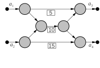
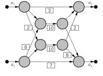
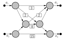
Figure 2: ${\cal N}_{1}$ (on the left) in Example 9, ${\cal N}_{2}$ (in the middle) in Example 10, and ${\cal N}_{3}$ (on the right) in Example 11, are similar networks, i.e., they have the same number of input arcs and the same number of output arcs. All missing capacities are the trivial lower bound $0$ and the trivial upper bound $K$ (a “very large number”).

Appendix B Appendix: Proofs and Supporting Lemmas for Section 4

Let $\mathbf{A}_{\text{in}}=\{a_{1},\ldots,a_{p}\}$ and $\mathbf{A}_{\text{out}}=\{a_{p+1},\ldots,a_{p+q}\}$ be fixed, where $p,q\geqslant 1$. Let $T\;:\;\mathscr{P}(\mathbf{A}_{\text{\rm in,out}})\,\to\,{\cal I}(\mathbb{R})$. If $[r,s]$ is an interval of real numbers for some $r\leqslant s$, we write $-[r,s]$ to denote the interval $[-s,-r]$. If $T(A)=[r,s]$ for some $A\subseteq\mathbf{A}_{\text{in,out}}$, we define $T^{\text{\rm min}}(A)=r$ and $T^{\text{\rm max}}(A)=s$.

The next two results, Lemma 12 and Lemma 13, are about tight typings $T$, independently of whether $T$ is sound and/or complete for a network ${\cal N}$.

Lemma 12.

Let $T\;:\;\mathscr{P}(\mathbf{A}_{\text{\rm in,out}})\,\to\,{\cal I}(\mathbb{R})$ be a tight typing such that: $T(\varnothing)=T(\mathbf{A}_{\text{\rm in,out}})=[0,0]$.

Conclusion: For every two-part partition of $\mathbf{A}_{\text{\rm in,out}}$, say $A\uplus B=\mathbf{A}_{\text{\rm in,out}}$, if both $T(A)$ and $T(B)$ are defined, then $T(A)=-T(B)$.

Proof.

One particular case in the conclusion is when $A=\varnothing$ and $B=\mathbf{A}_{\text{\rm in,out}}$, so that trivially $A\uplus B=\mathbf{A}_{\text{\rm in,out}}$, which also implies $T(A)=-T(B)$.

Consider the general case when $\varnothing\neq A,B\subsetneq\mathbf{A}_{\text{\rm in,out}}$. From Section 3, $\mathsf{Poly}(T)$ is the polytope defined by $T$ and $\mathsf{Constraints}(T)$ is the set of linear inequalities induced by $T$. For every $(p+q)$-dimensional point $f\in\mathsf{Poly}(T)$, we have:

$$\sum\,f(\mathbf{A}_{\text{in}})\ -\ \sum\,f(\mathbf{A}_{\text{out}})\ =\ 0$$

because $T(\mathbf{A}_{\text{\rm in,out}})=\{0\}$ and therefore:

$$0\ \leqslant\ \sum\,\{\,a\;|\;a\in\mathbf{A}_{\text{in}}\,\}\ -\ \sum\,\{\,a\;|\;a\in\mathbf{A}_{\text{out}}\,\}\ \leqslant 0$$

are among the inequalities in $\mathsf{Constraints}(T)$. Consider arbitrary $\varnothing\neq A,B\subsetneq\mathbf{A}_{\text{\rm in,out}}$ such that $A\uplus B=\mathbf{A}_{\text{\rm in,out}}$. We can therefore write the equation:

$$\quad\sum\,f(A\cap\mathbf{A}_{\text{in}})\ +\ \sum\,f(B\cap\mathbf{A}_{\text{in}})\ -\ \sum\,f(A\cap\mathbf{A}_{\text{out}})\ \ -\ \sum\,f(B\cap\mathbf{A}_{\text{out}})=\ 0$$

Or, equivalently:

• $\displaystyle\sum\,f(A\cap\mathbf{A}_{\text{in}})\ -\ \sum\,f(A\cap\mathbf{A}_{\text{out}})=-\sum\,f(B\cap\mathbf{A}_{\text{in}})\ +\ \sum\,f(B\cap\mathbf{A}_{\text{out}})$

for every $f\in\mathsf{Poly}(T)$. Hence, relative to $\mathsf{Constraints}(T)$, $f$ maximizes (resp. minimizes) the left-hand side of equation $({\ddagger})$ iff $f$ maximizes (resp. minimizes) the right-hand side of $({\ddagger})$. Negating the right-hand side of $({\ddagger})$, we also have:

$f$ maximizes (resp. minimizes) $\sum f(A\cap\mathbf{A}_{\text{in}})-\sum f(A\cap\mathbf{A}_{\text{out}})$   if and only if
$f$ minimizes (resp. maximizes) $\sum\,f(B\cap\mathbf{A}_{\text{in}})-\sum f(B\cap\mathbf{A}_{\text{out}})$   and the two quantities are equal.

Because $T$ is tight, every point $f\in\mathsf{Poly}(T)$ which maximizes (resp. minimizes) the objective function:

$$\sum\,\{\,a\;|\;a\in A\cap\mathbf{A}_{\text{in}}\,\}\ -\ \sum\,\{\,a\;|\;a\in A\cap\mathbf{A}_{\text{out}}\,\}$$

must be such that:

$$T^{\text{\rm max}}(A)\ =\ \sum f(A\cap\mathbf{A}_{\text{in}})\ -\ \sum f(A\cap\mathbf{A}_{\text{out}})$$

$$\Bigl{(}\text{resp.\ \ }T^{\text{\rm min}}(A)\ =\ \sum f(A\cap\mathbf{A}_{\text{in}})\ -\ \sum f(A\cap\mathbf{A}_{\text{out}})\Bigr{)}$$

We can repeat the same reasoning for $B$. Hence, if $f\in\mathsf{Poly}(T)$ maximizes both sides of $({\ddagger})$, then:

$$T^{\text{\rm max}}(A)\ =\ +\sum f(A\cap\mathbf{A}_{\text{in}})\ -\ \sum f(A\cap\mathbf{A}_{\text{out}})$$

$$=\ -\sum f(B\cap\mathbf{A}_{\text{in}})\ +\ \sum f(B\cap\mathbf{A}_{\text{out}})$$

$$=\ -T^{\text{\rm min}}(B)$$

and, respectively, if $f\in\mathsf{Poly}(T)$ minimizes both sides of $({\ddagger})$, then:

$$T^{\text{\rm min}}(A)\ =\ +\sum f(A\cap\mathbf{A}_{\text{in}})\ -\ \sum f(A\cap\mathbf{A}_{\text{out}})$$

$$=\ -\sum f(B\cap\mathbf{A}_{\text{in}})\ +\ \sum f(B\cap\mathbf{A}_{\text{out}})$$

$$=\ -T^{\text{\rm max}}(B)$$

The preceding implies $T(A)=-T(B)$ and concludes the proof. ∎

Lemma 13.

Let $T\;:\;\mathscr{P}(\mathbf{A}_{\text{\rm in,out}})\,\to\,{\cal I}(\mathbb{R})$ be a tight typing such that $T(\varnothing)=T(\mathbf{A}_{\text{\rm in,out}})=[0,0]$.

Conclusion: For every two-part partition $A\uplus B=\mathbf{A}_{\text{\rm in,out}}$, if $T(A)$ is defined and $T(B)$ is undefined, then:

$$\min\;\theta(B)=-T^{\text{\rm max}}(A)\quad\text{and}\quad\max\;\theta(B)=-T^{\text{\rm min}}(A),$$

where the objective function $\theta(B):=\sum(B\cap\mathbf{A}_{\text{\rm in}})-\sum(B\cap\mathbf{A}_{\text{\rm out}})$ is minimized and maximized, respectively, w.r.t. $\mathsf{Constraints}(T)$.

Hence, if we extend the typing $T$ to a typing $T^{\prime}$ that includes the type assignment $T^{\prime}(B):=-T(A)$, then $T^{\prime}$ is a tight typing such that $\mathsf{Poly}(T)=\mathsf{Poly}(T^{\prime})$.

Proof.

If $T(A)=[r,s]$, then $r=\min\theta(A)$ and $s=\max\theta(A)$ where $\theta(A):=\sum(A\cap\mathbf{A}_{\text{\rm in}})-\sum(A\cap\mathbf{A}_{\text{\rm out}})$ is minimized/maximized w.r.t. $\mathsf{Constraints}(T)$. Consider the objective function $\Theta:=\theta(A)+\theta(B)$. Because $T(\mathbf{A}_{\text{\rm in,out}})=[0,0]$, we have $\min\Theta=0=\max\Theta$ where $\Theta$ is minimized/maximized w.r.t. $\mathsf{Constraints}(T)$. Think of $\Theta$ as defining a line through the origin of the $\bigl{(}\theta(A),\theta(B)\bigr{)}$-plane with slope $-45^{o}$ with, say, $\theta(A)$ the horizontal coordinate and $\theta(B)$ the vertical coordinate. Hence, $\min\theta(B)=-\max\theta(A)$ and $\max\theta(B)=-\min\theta(A)$, which implies the desired conclusion. ∎

Proof 14 (for part 1 in Theorem 4).

Let ${\cal N}=(\mathbf{N},\mathbf{A})$ be a one-node flow network, i.e., $\mathbf{N}=\{\nu\}$ with all input arcs in $\mathbf{A}_{\text{in}}$ and all output arcs in $\mathbf{A}_{\text{out}}$ incident to the single node $\nu$. Algorithm 1 computes a principal typing for ${\cal N}$ and Lemma 15 proves its correctness.

Algorithm 1  Calculate Principal Typing for One-Node Network ${\cal N}$

1:algorithm name: $\mathsf{OneNodePT}$

2:input: one-node network ${\cal N}$ with input/output arcs $\mathbf{A}_{\text{in,out}}=\mathbf{A}_{\text{in}}\uplus\mathbf{A}_{\text{out}}$

3:         and lower-bound and upper-bound capacities $\underline{\bm{c}},\overline{\bm{c}}:\mathbf{A}_{\text{in,out}}\to\mathbb{R}_{+}$

4:output: principal typing $T:\mathscr{P}(\mathbf{A}_{\text{\rm in,out}})\to{\cal I}(\mathbb{R})$ for ${\cal N}$

5: 

6:$T(\varnothing)\ :=\ [0,0]$

7:$T(\mathbf{A}_{\text{\rm in,out}})\ :=\ [0,0]$

8:for every two-part partition $A\uplus B=\mathbf{A}_{\text{in,out}}$ with $A\neq\varnothing\neq B$ do

9:     $A_{\text{in}}:=A\cap\mathbf{A}_{\text{in}}$; $A_{\text{out}}:=A\cap\mathbf{A}_{\text{out}}$

10:     $B_{\text{in}}:=B\cap\mathbf{A}_{\text{in}}$; $B_{\text{out}}:=B\cap\mathbf{A}_{\text{out}}$

11:      $r_{1}:=-\min\bigl{\{}\sum\overline{\bm{c}}(B_{\text{in}})-\sum\underline{\bm{c}}(B_{\text{out}}),\ \sum\overline{\bm{c}}(A_{\text{out}})-\sum\underline{\bm{c}}(A_{\text{in}})\bigr{\}}$

12:      $r_{2}:=+\min\bigl{\{}\sum\overline{\bm{c}}(A_{\text{in}})-\sum\underline{\bm{c}}(A_{\text{out}}),\ \sum\overline{\bm{c}}(B_{\text{out}})-\sum\underline{\bm{c}}(B_{\text{in}})\bigr{\}}$

13:     $T(A)\ :=\ [r_{1},r_{2}]$

14:end for

15:return $T$

Lemma 15 (Principal Typings for One-Node Networks).

Let ${\cal N}$ be a network with one node, input arcs $\mathbf{A}_{\text{\rm in}}$, output arcs $\mathbf{A}_{\text{\rm out}}$, and lower-bound and upper-bound capacities $\underline{\bm{c}},\overline{\bm{c}}:\mathbf{A}_{\text{\rm in}}\uplus\mathbf{A}_{\text{\rm out}}\to\mathbb{R}_{+}$.

Conclusion: $\mathsf{OneNodePT}({\cal N})$ is a principal typing for ${\cal N}$.

Proof.

Let $A\uplus B=\mathbf{A}_{\text{in,out}}$ be an arbitrary two-part partition of $\mathbf{A}_{\text{in,out}}$, with $A\neq\varnothing\neq B$. Let $A_{\text{in}}:=A\cap\mathbf{A}_{\text{in}}$, $A_{\text{out}}:=A\cap\mathbf{A}_{\text{out}}$, $B_{\text{in}}:=B\cap\mathbf{A}_{\text{in}}$, and $B_{\text{out}}:=B\cap\mathbf{A}_{\text{out}}$. Define the non-negative numbers:

$$s_{\text{in}}\ :=\ \sum\underline{\bm{c}}(A_{\text{in}})\qquad s^{\prime}_{\text{in}}\ :=\ \sum\overline{\bm{c}}(A_{\text{in}})$$

$$s_{\text{out}}\ :=\ \sum\underline{\bm{c}}(A_{\text{out}})\quad s^{\prime}_{\text{out}}\ :=\ \sum\overline{\bm{c}}(A_{\text{out}})$$

$$t_{\text{in}} := \sum\underline{\bm{c}}(B_{\text{in}})\qquad t^{\prime}_{\text{in}} := \sum\overline{\bm{c}}(B_{\text{in}})$$

$$t_{\text{out}} := \sum\underline{\bm{c}}(B_{\text{out}})\quad t^{\prime}_{\text{out}} := \sum\overline{\bm{c}}(B_{\text{out}})$$

Although tedious and long, one approach to complete the proof is to exhaustively consider all possible orderings of the 8 values just defined, using the standard ordering on real numbers. Cases that do not allow any feasible flow can be eliminated from consideration; for feasible flows to be possible, we can assume that:

$$s_{\text{in}}\leqslant s^{\prime}_{\text{in}},\quad s_{\text{out}}\leqslant s^{\prime}_{\text{out}},\quad t_{\text{in}}\leqslant t^{\prime}_{\text{in}},\quad t_{\text{out}}\leqslant t^{\prime}_{\text{out}},\quad$$

and also assume that:

$$s_{\text{in}}+t_{\text{in}}\leqslant s^{\prime}_{\text{out}}+t^{\prime}_{\text{out}},\quad s_{\text{out}}+t_{\text{out}}\leqslant s^{\prime}_{\text{in}}+t^{\prime}_{\text{in}},\quad$$

thus reducing the total number of cases to consider. We consider the intervals $[s_{\text{in}},s^{\prime}_{\text{in}}]$, $[s_{\text{out}},s^{\prime}_{\text{out}}]$, $[t_{\text{in}},t^{\prime}_{\text{in}}]$, and $[t_{\text{out}},t^{\prime}_{\text{out}}]$, and their relative positions, under the preceding assumptions. Define the objective $\theta(A)$:

$$\theta(A)\ :=\ \sum A_{\text{in}}-\sum A_{\text{out}}.$$

If $T$ is a principal typing for ${\cal N}$, and therefore tight, with $T(A)=[r_{1},r_{2}]$, then $r_{1}$ is the minimum possible feasible value of $\theta(A)$ and $r_{2}$ is the maximum possible feasible value of $\theta(A)$ relative to $\mathsf{Constraints}(T)$.

We omit the details of the just-outlined exhaustive proof by cases. Instead, we argue for the correctness of $\mathsf{OneNodePT}$ more informally. It is helpful to consider the particular case when all lower-bound capacities are zero, i.e., the case when $s_{\text{in}}=s_{\text{out}}=t_{\text{in}}=t_{\text{out}}=0$. In this case, it is easy to see that:

$$r_{1}\ =\ -\min\bigl{\{}\sum\overline{\bm{c}}(B_{\text{in}}),\sum\overline{\bm{c}}(A_{\text{out}})\bigr{\}}\quad \text{maximum amount entering at $B_{\text{in}}$ and exiting at $A_{\text{out}}$},$$

$$\text{while minimizing amount entering at $A_{\text{in}}$},$$

$$r_{2}\ =\ +\min\bigl{\{}\sum\overline{\bm{c}}(A_{\text{in}}),\sum\overline{\bm{c}}(B_{\text{out}})\bigr{\}}\quad \text{maximum amount entering at $A_{\text{in}}$ and exiting at $B_{\text{out}}$},$$

$$\text{while minimizing amount exiting at $A_{\text{out}}$},$$

which are exactly the endpoints of the type $T(A)$ returned by $\mathsf{OneNodePT}({\cal N})$ in the particular case when all lower-bounds are zero.

Consider now the case when some of the lower-bounds are not zero. To determine the maximum throughput $r_{2}$ using the arcs of $A$, we consider two quantities:

$$r_{2}^{\prime}:=\sum\overline{\bm{c}}(A_{\text{in}})-\sum\underline{\bm{c}}(A_{\text{out}})\quad\text{and}\quad r_{2}^{\prime\prime}:=\sum\overline{\bm{c}}(B_{\text{out}})-\sum\underline{\bm{c}}(B_{\text{in}}).$$

It is easy to see that $r_{2}^{\prime}$ is the flow that is simultaneously maximized at $A_{\text{in}}$ and minimized at $A_{\text{out}}$, provided that $r_{2}^{\prime}\leqslant r_{2}^{\prime\prime}$, i.e., the whole amount $r_{2}^{\prime}$ can be made to enter at $A_{\text{in}}$ and to exit at $B_{\text{out}}$. However, if $r_{2}^{\prime}>r_{2}^{\prime\prime}$, then only the amount $r_{2}^{\prime\prime}$ can be made to enter at $A_{\text{in}}$ and to exit at $B_{\text{out}}$. Hence, the desired value of $r_{2}$ is $\min\{r_{2}^{\prime},r_{2}^{\prime\prime}\}$, which is exactly the higher endpoint of the type $T(A)$ returned by $\mathsf{OneNodePT}({\cal N})$. A similar argument, here omitted, is used again to determine the minimum throughput $r_{1}$ using the arcs of $A$. ∎

Complexity of $\mathsf{OneNodePT}$.

We estimate the run-time of $\mathsf{OneNodePT}$ as a function of: $d=|\,\mathbf{A}_{\text{in,out}}\,|\geqslant 2$, the number of input/output arcs, also assuming that there is at least one input arc and one output arc in ${\cal N}$. $\mathsf{OneNodePT}$ assigns the type/interval $[0,0]$ to $\varnothing$ and $\mathbf{A}_{\text{in,out}}$. For every $\varnothing\neq A\subsetneq\mathbf{A}_{\text{in,out}}$, it then computes a type $[r_{1},r_{2}]$, simultaneously for $A$ and its complement $B=\mathbf{A}_{\text{in,out}}-A$. (That $B$ is assigned $[-r_{2},-r_{1}]$ is not explicitly shown in Algorithm 1.) Hence, $\mathsf{OneNodePT}$ computes $(2^{d}-2)/2=(2^{d-1}-1)$ such types/intervals, each involving $8$ summations and $4$ subtractions, in lines 11 and 12, on the lower-bound capacities ($d$ of them) and upper-bound capacities ($d$ of them) of the input/output arcs. The run-time complexity of $\mathsf{OneNodePT}$ is therefore ${\cal O}\bigl{(}2^{d}\bigr{)}$.

Proof 16 (for part 2 in Theorem 4).

Given a principal typing $T$ for network ${\cal N}$ with arcs $\mathbf{A}=\mathbf{A}_{\text{in}}\uplus\mathbf{A}_{\text{out}}\uplus\mathbf{A}_{\text{\#}}$, together with $a^{+}\in\mathbf{A}_{\text{in}}$ and $a^{-}\in\mathbf{A}_{\text{out}}$, we need to compute a principal typing $T^{\prime}$ for the network $\mathsf{Bind}\bigl{(}a,{\cal N}\bigr{)}$. This is carried out by Algorithm 2 below and its correctness established by Lemma 17.

Algorithm 2  Bind One Input-Output Pair Efficiently

1:algorithm name: $\mathsf{BindPT}_{1}$

2:input: principal typing $T:\mathscr{P}(\mathbf{A}_{\text{\rm in,out}})\to{\cal I}(\mathbb{R})$,  $a^{+}\in\mathbf{A}_{\text{\rm in}}$,  $a^{-}\in\mathbf{A}_{\text{\rm out}}$

3:         where for every two-part partition $A\uplus B=\mathbf{A}^{\prime}_{\text{\rm in,out}}:={\mathbf{A}_{\text{\rm in,out}}}-\{a^{+},a^{-}\}$,

4:         either both $T(A)$ and $T(B)$ are defined or both $T(A)$ and $T(B)$ are undefined

5:output: principal typing $T^{\prime}:\mathscr{P}(\mathbf{A}^{\prime}_{\text{\rm in,out}})\to{\cal I}(\mathbb{R})$

6:           where $\mathsf{Poly}(T^{\prime})=[\mathsf{Poly}(\mathsf{Constraints}(T)\cup\{a^{+}=a^{-}\})]_{\mathbf{A}^{\prime}_{\text{\rm in,out}}}$

7: 

8:Definition of intermediate typing $T_{1}:\mathscr{P}(\mathbf{A}^{\prime}_{\text{\rm in,out}})\to{\cal I}(\mathbb{R})$

9: $T_{1}\ :=\ [T]_{\mathscr{P}(\mathbf{A}^{\prime}_{\text{\rm in,out}})}$,

10:i.e., every type assigned by $T$ to a set $A$ such that $A\cap\{a^{+},a^{-}\}\neq\varnothing$ is omitted in $T_{1}$

11: 

12:Definition of intermediate typing $T_{2}:\mathscr{P}(\mathbf{A}^{\prime}_{\text{\rm in,out}})\to{\cal I}(\mathbb{R})$

13: $T_{2}\ :=\ T_{1}\bigl{[}\mathbf{A}^{\prime}_{\text{\rm in,out}}\mapsto[0,0]\bigr{]}$

14:i.e., the type assigned by $T_{1}$ to $\mathbf{A}^{\prime}_{\text{\rm in,out}}$, if any, is changed to the type $[0,0]$ in $T_{2}$

15: 

16:Definition of final typing $T^{\prime}:\mathscr{P}(\mathbf{A}^{\prime}_{\text{\rm in,out}})\to{\cal I}(\mathbb{R})$

17:for every two-part partition $A\uplus B=\mathbf{A}^{\prime}_{\text{in,out}}$ do

18:     if $T_{2}(A)$ is defined with $T_{2}(A)=[r_{1},s_{1}]$ and $T_{2}(B)$ is defined with $-T_{2}(B)=[r_{2},s_{2}]$ then

19:          $T^{\prime}(A):=[\max\{r_{1},r_{2}\},\min\{s_{1},s_{2}\}]$ ; $T^{\prime}(B):=-T^{\prime}(A)$

20:     else if both $T_{2}(A)$ and $T_{2}(B)$ are undefined then

21:         $T^{\prime}(A)$ is undefined ; $T^{\prime}(B)$ is undefined

22:     end if

23:end for

24:return $T^{\prime}$

Lemma 17 (Typing for Binding One Input/Output Pair).

Let $T:\mathscr{P}(\mathbf{A}_{\text{\rm in,out}})\to{\cal I}(\mathbb{R})$ be a principal typing for network ${\cal N}$, with input/output arcs $\mathbf{A}_{\text{\rm in,out}}=\mathbf{A}_{\text{\rm in}}\uplus\mathbf{A}_{\text{\rm out}}$, and let $a^{+}\in\mathbf{A}_{\text{\rm in}}$ and $a^{-}\in\mathbf{A}_{\text{\rm out}}$.

Conclusion: $\mathsf{BindPT}_{1}(a,T)$ is a principal typing for $\mathsf{Bind}\bigl{(}a,{\cal N}\bigr{)}$.

Proof.

Consider the intermediate typings $T_{1}$ and $T_{2}$ as defined in algorithm $\mathsf{BindPT}_{1}$:

$$T_{1},T_{2}:\mathscr{P}(\mathbf{A}^{\prime}_{\text{\rm in,out}})\to{\cal I}(\mathbb{R})\quad\text{where $\mathbf{A}^{\prime}_{\text{\rm in,out}}=\mathbf{A}_{\text{\rm in,out}}-\{a^{+},a^{-}\}$.}$$

The definitions of $T_{1}$ and $T_{2}$ can be repeated differently as follows. For every $A\subseteq\mathbf{A}_{\text{\rm in,out}}$:

$$T_{1}(A)\ :=\ \begin{cases}T(A)&\text{if $A\subseteq\mathbf{A}^{\prime}_{\text{\rm in,out}}$ and $T(A)$ is defined},\\ \text{undefined}\quad&\text{if $A\not\subseteq\mathbf{A}^{\prime}_{\text{\rm in,out}}$ or $T(A)$ is undefined},\end{cases}$$

$$T_{2}(A)\ :=\ \begin{cases}T_{1}(A)\qquad&\text{if $A\subsetneq\mathbf{A}^{\prime}_{\text{\rm in,out}}$ and $T_{1}(A)$ is defined},\\ [0,0]\qquad&\text{if $A=\mathbf{A}^{\prime}_{\text{\rm in,out}}$},\\ \text{undefined}\quad&\text{if $A\not\subseteq\mathbf{A}^{\prime}_{\text{\rm in,out}}$ or $T_{1}(A)$ is undefined}.\end{cases}$$

If $T$ is tight, then so is $T_{1}$. The only difference between $T_{1}$ and $T_{2}$ is that the latter includes the new type assignment $T_{2}(\mathbf{A}^{\prime}_{\text{\rm in,out}})=[0,0]$, which is equivalent to the constraint:

$$\sum\mathbf{A}^{\prime}_{\text{\rm in}}-\sum\mathbf{A}^{\prime}_{\text{\rm out}}=0,\qquad\text{where $\mathbf{A}^{\prime}_{\text{\rm in}}=\mathbf{A}_{\text{\rm in}}-\{a^{+}\}$ and $\mathbf{A}^{\prime}_{\text{\rm out}}=\mathbf{A}_{\text{\rm out}}-\{a^{-}\}$},$$

which, given the fact that $\sum\mathbf{A}_{\text{\rm in}}-\sum\mathbf{A}_{\text{\rm out}}=0$, is in turn equivalent to the constraint $a^{+}=a^{-}$. This implies the following equalities:

$$[\mathsf{Poly}(\mathsf{Constraints}(T)\cup\{a^{+}=a^{-}\})]_{\mathbf{A}^{\prime}_{\text{\rm in,out}}}\ =\ \mathsf{Poly}(\mathsf{Constraints}(T_{1})\cup\{\mathbf{A}^{\prime}_{\text{\rm in}}=\mathbf{A}^{\prime}_{\text{\rm out}}\})$$

$$=\ \mathsf{Poly}(\mathsf{Constraints}(T_{2}))$$

$$=\ \mathsf{Poly}(T_{2})$$

Hence, if $T$ is a principal typing for ${\cal N}$, then $T_{2}$ is a principal typing for $\mathsf{Bind}\bigl{(}a,{\cal N}\bigr{)}$. It remains to show that $T^{\prime}$ as defined in algorithm $\mathsf{BindPT}_{1}$ is the tight version of $T_{2}$.

We define an additional typing $T_{3}:\mathscr{P}(\mathbf{A}^{\prime}_{\text{\rm in,out}})\to{\cal I}(\mathbb{R})$ as follows – for the purposes of this proof only, $T_{3}$ is not computed by algorithm $\mathsf{BindPT}_{1}$. For every $A\subseteq\mathbf{A}^{\prime}_{\text{\rm in,out}}$ for which $T_{2}(A)$ is defined, let the objective $\theta_{A}$ be $\sum(A\cap\mathbf{A}^{\prime}_{\text{\rm in}})-\sum(A\cap\mathbf{A}^{\prime}_{\text{\rm out}})$ and let:

$$T_{3}(A)\ :=\ [r,s]\qquad\text{where $r=\min\theta_{A}$ and $s=\max\theta_{A}$ relative to $\mathsf{Constraints}(T_{2})$}.$$

$T_{3}$ is obtained from $T_{2}$ in an “expensive” process, because it uses a linear-programming algorithm to minimize/maximize the objectives $\theta_{A}$. Clearly $\mathsf{Poly}(T_{2})=\mathsf{Poly}(T_{3})$. Moreover, $T_{3}$ is guaranteed to be tight by the definitions and results in Section 2 – we leave to the reader the straightforward details showing that $T_{3}$ is tight. In particular, for every $A\subseteq\mathbf{A}^{\prime}_{\text{\rm in,out}}$ for which $T_{2}(A)$ is defined, it holds that $T_{3}(A)\subseteq T_{2}(A)$. Hence, for every $A\uplus B=\mathbf{A}^{\prime}_{\text{\rm in,out}}$ for which $T_{2}(A)$ and $T_{2}(B)$ are both defined:

(1) $$T_{3}(A)\ \subseteq\ T_{2}(A)\,\cap\,-T_{2}(B),$$

since $T_{3}(A)=-T_{3}(B)$ by Lemma 12. Keep in mind that:

(2) $$\text{$\mathsf{Poly}(T_{3})$ is the largest polytope satisfying $\mathsf{Constraints}(T_{2})$},$$

and every other polytope satisfying $\mathsf{Constraints}(T_{2})$ is a subset of $\mathsf{Poly}(T_{3})$. We define one more typing $T_{4}:\mathscr{P}(\mathbf{A}^{\prime}_{\text{\rm in,out}})\to{\cal I}(\mathbb{R})$ by appropriately restricting $T_{2}$; namely, for every two-part partition $A\uplus B=\mathbf{A}^{\prime}_{\text{\rm in,out}}$:

$$T_{4}(A)\ :=\ \begin{cases}\phantom{-}T_{2}(A)\,\cap\,-T_{2}(B)\quad&\text{if both $T_{2}(A)$ and $T_{2}(B)$ are defined},\\ \phantom{-}\text{undefined}&\text{if both $T_{2}(A)$ and $T_{2}(B)$ are undefined}.\end{cases}$$

Hence, $\mathsf{Poly}(T_{4})$ satisfies $\mathsf{Constraints}(T_{2})$, so that also for every $A\subseteq\mathbf{A}^{\prime}_{\text{\rm in,out}}$ for which $T_{4}(A)$ is defined, we have $T_{3}(A)\supseteq T_{4}(A)$, by (2) above. Hence, for every $A\uplus B=\mathbf{A}^{\prime}_{\text{\rm in,out}}$ for which $T_{4}(A)$ and $T_{4}(B)$ are both defined, we have:

(3) $$T_{3}(A)\ \supseteq\ T_{4}(A)\ =\ -T_{4}(B)\ =\ T_{2}(A)\,\cap\,-T_{2}(B).$$

Putting (1) and (3) together:

$$T_{2}(A)\,\cap\,-T_{2}(B)\ \subseteq\ T_{3}(A)\ \subseteq\ \ T_{2}(A)\,\cap\,-T_{2}(B),$$

which implies $T_{3}(A)=T_{2}(A)\,\cap\,-T_{2}(B)=T_{4}(A)$. Hence, also, for every $A\subseteq\mathbf{A}^{\prime}_{\text{\rm in,out}}$ for which $T_{3}(A)$ is defined, $T_{3}(A)=T_{4}(A)$. This implies $\mathsf{Poly}(T_{3})=\mathsf{Poly}(T_{4})$ and that $T_{4}$ is tight. $T_{4}$ is none other than $T^{\prime}$ in algorithm $\mathsf{BindPT}_{1}$, thus concluding the proof of the first part in the conclusion of the proposition. For the second part, it is readily checked that if $T$ is a total typing, then so is $T^{\prime}$ (details omitted). ∎

Complexity of $\mathsf{BindPT}_{1}$.

We measure the run-time of $\mathsf{BindPT}_{1}$ by the number of bookkeeping steps (whether a variable/arc name is in a set or not) and the number of number-comparisons (there are no additions and subtractions in $\mathsf{BindPT}_{1}$) as a function of:

• $|\,\mathbf{A}_{\text{in,out}}\,|$, the number of input/output arcs,

• $|\,T\,|$, the number of assigned types in the initial typing $T$.

We consider each of the three parts separately:

1. The first part, line 9, runs in ${\cal O}\bigl{(}|\,\mathbf{A}_{\text{in,out}}\,|\cdot|\,T\,|\bigr{)}$ time, according to the following reasoning. Suppose the types of $T$ are organized as a list with $|\,T\,|$ entries, which we can scan from left to right. The algorithm removes every type assigned to a subset $A\subseteq\mathbf{A}_{\text{in,out}}$ intersecting $\{a^{+},a^{-}\}$. There are $|\,T\,|$ types to be inspected, and the subset $A$ to which $T(A)$ is assigned has to be checked that it does not contain $a^{+}$ or $a^{-}$. The resulting intermediate typing $T_{1}$ is such that $|\,T_{1}\,|\leqslant|\,T\,|$.

2. The second part of $\mathsf{BindPT}_{1}$, line 13, runs in ${\cal O}\bigl{(}|\,\mathbf{A}^{\prime}_{\text{in,out}}\,|\cdot|\,T_{1}\,|\bigr{)}$ time. It inspects each of the $|\,T_{1}\,|$ types, looking for one assigned to $\mathbf{A}^{\prime}_{\text{in,out}}$, each such inspection requiring $|\,\mathbf{A}^{\prime}_{\text{in,out}}\,|$ comparison steps. If it finds such a type, it replaces it by $[0,0]$. If it does not find such a type, it adds the type assignment $\{\mathbf{A}^{\prime}_{\text{in,out}}\mapsto[0,0]\}$. The resulting intermediate typing $T_{2}$ is such that $|\,T_{2}\,|=|\,T_{1}\,|$ or $|\,T_{2}\,|=1+|\,T_{1}\,|$.

3. The third part, from line 17 to line 23, runs in ${\cal O}\bigl{(}|\,\mathbf{A}^{\prime}_{\text{in,out}}\,|\cdot|\,T_{2}\,|^{2}\bigr{)}$ time. For every type $T_{2}(A)$, it looks for a type $T_{2}(B)$ in at most $|\,T_{2}\,|$ scanning steps, such that $A\uplus B=\mathbf{A}^{\prime}_{\text{in,out}}$ in at most $|\,\mathbf{A}^{\prime}_{\text{in,out}}\,|$ comparison steps; if and when it finds a type $T_{2}(B)$, which is guaranteed to be defined, it carries out the operation in line 19.

Adding the estimated run-times in the three parts, the overall run-time of $\mathsf{BindPT}_{1}$ is ${\cal O}\bigl{(}|\,\mathbf{A}_{\text{in,out}}\,|\cdot|\,T\,|^{2}\bigr{)}$. Let $\delta=|\,\mathbf{A}_{\text{in,out}}\,|\geqslant 2$. In the particular case when $T$ is a total typing which therefore assigns a type to each of the $2^{\delta}$ subsets of $\mathbf{A}_{\text{in,out}}$, the overall run-time of $\mathsf{BindPT}_{1}$ is ${\cal O}\bigl{(}\delta\cdot 2^{2\delta}\bigr{)}={\cal O}\bigl{(}2^{\log\delta+2\delta}\bigr{)}=2^{{\cal O}(\delta)}$.

Note there are no arithmetical steps (addition, multiplication, etc.) in the execution of $\mathsf{BindPT}_{1}$; besides the bookkeeping involved in partitioning $\mathbf{A}^{\prime}_{\text{in,out}}$ in two disjoint parts, $\mathsf{BindPT}_{1}$ uses only comparison of numbers in line 19.

Proof 18 (for part 3 in Theorem 4).

Let ${\cal N}^{\prime}$ and ${\cal N}^{\prime\prime}$ be two separate networks, with arcs $\mathbf{A}^{\prime}=\mathbf{A}^{\prime}_{\text{in}}\uplus\mathbf{A}^{\prime}_{\text{out}}\uplus\mathbf{A}^{\prime}_{\text{\#}}$ and $\mathbf{A}^{\prime\prime}=\mathbf{A}^{\prime\prime}_{\text{in}}\uplus\mathbf{A}^{\prime\prime}_{\text{out}}\uplus\mathbf{A}^{\prime\prime}_{\text{\#}}$, respectively. The parallel addition of ${\cal N}^{\prime}$ and ${\cal N}^{\prime\prime}$, denoted $({\cal N}^{\prime}\,\bm{\|}\,{\cal N}^{\prime\prime})$, simply places ${\cal N}^{\prime}$ and ${\cal N}^{\prime\prime}$ next to each other without connecting any of their external arcs. If ${\cal N}=({\cal N}^{\prime}\,\bm{\|}\,{\cal N}^{\prime\prime})$, then the input and output arcs of ${\cal N}$ are $\mathbf{A}^{\prime}_{\text{in}}\uplus\mathbf{A}^{\prime\prime}_{\text{in}}$ and $\mathbf{A}^{\prime}_{\text{out}}\uplus\mathbf{A}^{\prime\prime}_{\text{out}}$, respectively, and its internal arcs are $\mathbf{A}^{\prime}_{\text{\#}}\uplus\mathbf{A}^{\prime\prime}_{\text{\#}}$. If ${\cal N}^{\prime}$ and ${\cal N}^{\prime\prime}$ are each connected, we view ${\cal N}$ as a network with two separate connected components.

Let $T^{\prime}$ and $T^{\prime\prime}$ be principal typings for the two separate networks ${\cal N}^{\prime}$ and ${\cal N}^{\prime\prime}$. We define the the parallel addition of $T^{\prime}$ and $T^{\prime\prime}$ as follows:

$$(T^{\prime}\bm{\oplus}T^{\prime\prime})(A)\ :=\ \begin{cases}[0,0]\qquad&\text{if $A=\varnothing$ or $A=\mathbf{A}^{\prime}_{\text{\rm in,out}}\cup\mathbf{A}^{\prime\prime}_{\text{\rm in,out}}$},\\[4.30554pt] T^{\prime}(A)&\text{if $A\subseteq\mathbf{A}^{\prime}_{\text{\rm in,out}}$ and $T^{\prime}(A)$ is defined},\\[4.30554pt] T^{\prime\prime}(A)&\text{if $A\subseteq\mathbf{A}^{\prime\prime}_{\text{\rm in,out}}$ and $T^{\prime\prime}(A)$ is defined},\\[4.30554pt] \text{undefined}\qquad&\text{otherwise}.\end{cases}$$

Lemma 19 (Typing for Parallel Addition).

Let ${\cal N}^{\prime}$ and ${\cal N}^{\prime\prime}$ be two separate networks with external arcs $\mathbf{A}^{\prime}_{\text{\rm in,out}}=\mathbf{A}^{\prime}_{\text{\rm in}}\uplus\mathbf{A}^{\prime}_{\text{\rm out}}$ and $\mathbf{A}^{\prime\prime}_{\text{\rm in,out}}=\mathbf{A}^{\prime\prime}_{\text{\rm in}}\uplus\mathbf{A}^{\prime\prime}_{\text{\rm out}}$, respectively. Let $T^{\prime}$ and $T^{\prime\prime}$ be principal typings for ${\cal N}^{\prime}$ and ${\cal N}^{\prime\prime}$, respectively.

Conclusion: $(T^{\prime}\bm{\oplus}T^{\prime\prime})$ is a principal typing for the network $({\cal N}^{\prime}\,\bm{\|}\,{\cal N}^{\prime\prime})$.

Proof.

There is no communication between ${\cal N}^{\prime}$ and ${\cal N}^{\prime\prime}$. The conclusion of the proposition is a straightforward consequence of the definitions. All details omitted. ∎

The typing $(T^{\prime}\bm{\oplus}T^{\prime\prime})$ is partial even when $T^{\prime}$ and $T^{\prime\prime}$ are total typings. We need to define the total parallel addition of total typings which is another total typing. If $[r_{1},s_{1}]$ and $[r_{2},s_{1}]$ are intervals of real numbers for some $r_{1}\leqslant s_{1}$ and $r_{2}\leqslant s_{2}$, we write $[r_{1},s_{1}]+[r_{2},s_{2}]$ to denote the interval $[r_{1}+r_{2},s_{1}+s_{2}]$:

$$[r_{1},s_{1}]+[r_{2},s_{2}]\ :=\ \{\,t\in\mathbb{R}\;|\;r_{1}+r_{2}\leqslant t\leqslant s_{1}+s_{2}\,\}$$

Let $T^{\prime}$ and $T^{\prime\prime}$ be tight and total typings over disjoint sets of external arcs, $\mathbf{A}^{\prime}_{\text{\rm in,out}}=\mathbf{A}^{\prime}_{\text{\rm in}}\uplus\mathbf{A}^{\prime}_{\text{\rm out}}$ and $\mathbf{A}^{\prime\prime}_{\text{\rm in,out}}=\mathbf{A}^{\prime\prime}_{\text{\rm in}}\uplus\mathbf{A}^{\prime\prime}_{\text{\rm out}}$, respectively. We define the total parallel addition $(T^{\prime}\bm{\oplus_{\text{\rm t}}}T^{\prime\prime})$ of the typings $T^{\prime}$ and $T^{\prime\prime}$ as follows. For every $A\subseteq\mathbf{A}^{\prime}_{\text{\rm in,out}}\cup\mathbf{A}^{\prime\prime}_{\text{\rm in,out}}$:

$$(T^{\prime}\bm{\oplus_{\text{\rm t}}}T^{\prime\prime})(A)\ :=\ \begin{cases}[0,0]\qquad&\text{if $A=\varnothing$ or $A=\mathbf{A}^{\prime}_{\text{\rm in,out}}\cup\mathbf{A}^{\prime\prime}_{\text{\rm in,out}}$},\\[4.30554pt] T^{\prime}(A^{\prime})+T^{\prime\prime}(A^{\prime\prime})&\text{if $A=A^{\prime}\uplus A^{\prime\prime}$ with $A^{\prime}=A\cap\mathbf{A}^{\prime}_{\text{\rm in,out}}$ and $A^{\prime\prime}=A\cap\mathbf{A}^{\prime\prime}_{\text{\rm in,out}}$.}\end{cases}$$

Lemma 20 (Total Typing for Parallel Addition).

Let ${\cal N}^{\prime}$ and ${\cal N}^{\prime\prime}$ be two separate networks with external arcs $\mathbf{A}^{\prime}_{\text{\rm in,out}}=\mathbf{A}^{\prime}_{\text{\rm in}}\uplus\mathbf{A}^{\prime}_{\text{\rm out}}$ and $\mathbf{A}^{\prime\prime}_{\text{\rm in,out}}=\mathbf{A}^{\prime\prime}_{\text{\rm in}}\uplus\mathbf{A}^{\prime\prime}_{\text{\rm out}}$, respectively. Let $T^{\prime}$ and $T^{\prime\prime}$ be principal typings for ${\cal N}^{\prime}$ and ${\cal N}^{\prime\prime}$, respectively.

Conclusion: $(T^{\prime}\bm{\oplus_{\text{\rm t}}}T^{\prime\prime})$ is a tight, sound, and complete typing for the network $({\cal N}^{\prime}\,\bm{\|}\,{\cal N}^{\prime\prime})$. Moreover, if $T^{\prime}$ and $T^{\prime\prime}$ are total (because ${\cal N}^{\prime}$ and ${\cal N}^{\prime\prime}$ are each a connected network), then $(T^{\prime}\bm{\oplus_{\text{\rm t}}}T^{\prime\prime})$ is also total – but not locally total, because $({\cal N}^{\prime}\,\bm{\|}\,{\cal N}^{\prime\prime})$ consists of two separate components.

Proof.

Similar to the proof of Lemma 19. Straightforward consequence from the fact there is no communication between ${\cal N}^{\prime}$ and ${\cal N}^{\prime\prime}$. All details omitted. ∎

Complexity of $\bm{\oplus}$ and $\bm{\oplus_{\text{\rm t}}}$.

The cost of $(T^{\prime}\bm{\oplus}T^{\prime\prime})(A)$ is the cost of determining whether $A\subseteq\mathbf{A}^{\prime}_{\text{\rm in,out}}$ or $A\subseteq\mathbf{A}^{\prime\prime}_{\text{\rm in,out}}$, which is therefore a number of bookkeeping steps linear in $|\,\mathbf{A}^{\prime}_{\text{\rm in,out}}\,|+|\,\mathbf{A}^{\prime\prime}_{\text{\rm in,out}}\,|$. There are no arithmetical operations in the computation of $(T^{\prime}\bm{\oplus}T^{\prime\prime})(A)$.

The cost of $(T^{\prime}\bm{\oplus_{\text{\rm t}}}T^{\prime\prime})(A)$ is a little more involved. In addition to the bookkeeping steps, it includes two number-additions after the two subsets $A^{\prime}=A\cap\mathbf{A}^{\prime}_{\text{\rm in,out}}$ and $A^{\prime\prime}=A\cap\mathbf{A}^{\prime\prime}_{\text{\rm in,out}}$ are determined.

We need one more operation on typings, $\mathsf{BindPT}$, to define Algorithm 3 precisely. $\mathsf{BindPT}$ uses operations $\bm{\oplus_{\text{\rm t}}}$ defined above and $\mathsf{BindPT}_{1}$ defined in the proof of part 2 of Theorem 4. Let ${\cal N}$ be a network with $k\geqslant 2$ components, say, ${\cal N}={\cal M}_{1}\,\bm{\|}\,{\cal M}_{2}\,\bm{\|}\,\cdots\,\bm{\|}\,{\cal M}_{k}$, with input arcs $\mathbf{A}_{\text{in}}$ and output arcs $\mathbf{A}_{\text{out}}$. Let $T$ be a principal typing for ${\cal N}$, say, $T=U_{1}\bm{\oplus}U_{2}\bm{\oplus}\cdots\bm{\oplus}U_{k}$, where $U_{i}$ is a principal typing for component ${\cal M}_{i}$. Let $a^{+}\in\mathbf{A}_{\text{in}}$ and $a^{-}\in\mathbf{A}_{\text{out}}$.

There are two cases: (1) The two halves $a^{+}$ and $a^{-}$ occur in the same component ${\cal M}_{i}$, and (2) the two halves occur in two separate components ${\cal M}_{i}$ and ${\cal M}_{j}$ with $i\neq j$. We define $\mathsf{BindPT}(a,T)$ by:

$$\mathsf{BindPT}(a,T)\ :=\ \begin{cases}\bigoplus\bigl{(}\{U_{1},\ldots,U_{k}\}-\{U_{i}\}\bigr{)}\ \oplus\ \mathsf{BindPT}_{1}(a,U_{i})\quad&\text{if $a^{+}$ and $a^{-}$ are both in}\\ \quad&\text{component ${\cal M}_{i}$,}\\[5.16663pt] \bigoplus\bigl{(}\{U_{1},\ldots,U_{k}\}-\{U_{i},U_{j}\}\bigr{)}\ \oplus\ \mathsf{BindPT}_{1}(a,U_{i}\bm{\oplus_{\text{\rm t}}}U_{j})\quad&\text{if $a^{+}$ and $a^{-}$ are in two}\\ \quad&\text{separate components,}\\ \quad&\text{${\cal M}_{i}$ and ${\cal M}_{j}$, with $i\neq j$.}\end{cases}$$

Complexity of $\mathsf{BindPT}$.

Part of the information given to $\mathsf{BindPT}$ is whether $a^{+}$ and $a^{-}$ are in the same component ${\cal M}_{i}$ or in two different components ${\cal M}_{i}$ and ${\cal M}_{j}$ of ${\cal N}$. This is a bookkeeping task that can be included in the execution of Algorithm 3. Suppose $\delta\geqslant 2$ is an upper bound on the number of external arcs of ${\cal M}_{i}$ (in the first case) or $({\cal M}_{i}\,\bm{\|}\,{\cal M}_{j})$ (in the second case).

In the first case, the cost of executing $\mathsf{BindPT}(a,T)$ is the cost of executing $\mathsf{BindPT}_{1}(a,T)$, which is ${\cal O}\bigl{(}\delta\cdot 2^{2\delta}\bigr{)}=2^{{\cal O}(\delta)}$. In the second case, we need to add the initial cost of computing $U_{i}\bm{\oplus_{\text{\rm t}}}U_{j}$, which consists of performing two additions for each of $2^{\delta}-2$ subsets (of the external arcs of $({\cal M}_{i}\,\bm{\|}\,{\cal M}_{j})$, i.e., the set of arcs/variables over which $U_{i}\bm{\oplus_{\text{\rm t}}}U_{j}$ is defined). This initial cost is ${\cal O}\bigl{(}2^{\delta}\bigr{)}$, so that the total of executing $\mathsf{BindPT}(a,T)$ in the second case is again $2^{{\cal O}(\delta)}$.

Algorithm 3  Calculate a Principal Typing for Network ${\cal N}$

1:algorithm name: $\mathsf{CompPT}$

2:input: ${\cal N}=(\mathbf{N},\mathbf{A})$ is a connected flow network,

3:         $\sigma=b_{1}b_{2}\cdots b_{m}$ is an ordering of the internal arcs of ${\cal N}$ (a “binding schedule”),

4:         where $\mathbf{N}=\{\nu_{1},\nu_{2},\ldots,\nu_{n}\}$,   $\mathbf{A}=\mathbf{A}_{\text{in,out}}\uplus\mathbf{A}_{\text{\#}}$,  and  $\mathbf{A}_{\text{\#}}=\{b_{1},b_{2},\ldots,b_{m}\}$

5:output: principal typing $T$ for ${\cal N}$

6: 

7: ${\cal N}_{0}\ :=\ {\cal M}_{1}\,\bm{\|}\,{\cal M}_{2}\,\bm{\|}\,\cdots\,\bm{\|}\,{\cal M}_{n}$

8:  where $\{{\cal M}_{1},{\cal M}_{2},\ldots,{\cal M}_{n}\}=\mathsf{BreakUp}({\cal N})$

9: $T_{0}\ :=\ \mathsf{OneNodePT}({\cal M}_{1})\bm{\oplus}\mathsf{OneNodePT}({\cal M}_{2})\bm{\oplus}\cdots\bm{\oplus}\mathsf{OneNodePT}({\cal M}_{n})$

10:for every $k=0,1,\ldots,m-1$ do

11:      ${\cal N}_{k+1}\ :=\ \mathsf{Bind}\bigl{(}b_{k+1},{\cal N}_{k}\bigr{)}$

12:     $T_{k+1}\ :=\ \mathsf{BindPT}(b_{k+1},T_{k})$

13:end for

14:$T:=T_{m}$

15:return $T$

Lemma 21 (Inferring Principal Typings).

Let ${\cal N}$ be a connected flow network and let  $\sigma=b_{1}b_{2}\cdots b_{m}$  be an ordering of all the internal arcs of ${\cal N}$ (a “binding schedule”). Then the typing $T=\mathsf{CompPT}({\cal N},\sigma)$ is principal for network ${\cal N}$.

Proof.

It suffices to show that, for every $k=0,1,2,\ldots,m$, the typing $T_{k}$ is principal for ${\cal N}_{k}$, where $T_{k}$ consists of the parallel addition of as many principal typings as there are components in ${\cal N}_{k}$. This is true for $k=0$ by Lemmas 15 and 19, and is true again for each $k\geqslant 1$ by Lemmas 17 and 20. The final ${\cal N}_{m}$ consists of a single component (itself) and the resulting typing $T_{m}$ is therefore total. ∎

Let ${\cal N}$ be a connected network and $\sigma=b_{1}b_{2}\cdots b_{m}$ an ordering of the internal arcs of ${\cal N}$. As in line 7 of Algorithm 3, let:

$${\cal N}_{0}\ =\ {\cal M}_{1}\,\bm{\|}\,{\cal M}_{2}\,\bm{\|}\,\cdots\,\bm{\|}\,{\cal M}_{n}$$

where $\{{\cal M}_{1},{\cal M}_{2},\ldots,{\cal M}_{n}\}=\mathsf{BreakUp}({\cal N})$, and as in line 11, let:

$${\cal N}_{1}\ =\ \mathsf{Bind}\bigl{(}b_{1},{\cal N}_{0}\bigr{)},\ {\cal N}_{2}\ =\ \mathsf{Bind}\bigl{(}b_{2},{\cal N}_{1}\bigr{)},\ \ldots\ ,\ {\cal N}_{m}\ =\ \mathsf{Bind}\bigl{(}b_{m},{\cal N}_{m-1}\bigr{)}.$$

These ${\cal N}_{0},{\cal N}_{1},\ldots,{\cal N}_{m}$ are the same as in Section 4.

Complexity of $\mathsf{CompPT}$.

We ignore the effort to define the initial network ${\cal N}_{0}$ and then to update it to ${\cal N}_{1},{\cal N}_{2},\ldots,{\cal N}_{m}$. In fact, beyond the initial ${\cal N}_{0}$, which we use to define the initial typing $T_{0}$, the intermediate networks ${\cal N}_{1},{\cal N}_{2},\ldots,{\cal N}_{m}$ play no role in the computation of the final typing $T=T_{m}$ returned by $\mathsf{CompPT}$. We included the intermediate networks in the algorithm for clarity and to make explicit the correspondence between $T_{k}$ and ${\cal N}_{k}$ for every $1\leqslant k\leqslant m$ (which is used in the proof of Lemma 21).

The run-time complexity of $\mathsf{CompPT}$ is dominated by the computation of type assignments (involving arithmetical additions, subtractions, and comparisons), not by the bookkeeping steps. Let $\delta={\mathit{index}}(\sigma)$.

There are at most $n\cdot 2^{\delta}$ type assignments in $T_{0}$ in line 9. In the for-loop from line 10 to line 13, $\mathsf{CompPT}$ calls $\mathsf{BindPT}$ once in each of $m$ iterations, for a total of $m$ calls. Each such call to $\mathsf{BindPT}$ runs in time ${\cal O}\bigl{(}\delta\cdot 2^{2\delta}\bigr{)}=2^{{\cal O}(\delta)}$. Hence, the run-time complexity of $\mathsf{CompPT}$ is:

$${\cal O}\bigl{(}n\cdot 2^{\delta}+m\cdot\delta\cdot 2^{2\delta}\bigr{)}={\cal O}\bigl{(}(m+n)\cdot\delta\cdot 2^{2\delta}\bigr{)}=(m+n)\cdot 2^{{\cal O}(\delta)}.$$

Appendix C Appendix: Proofs and Supporting Lemmas for Section 5

We need a few definitions and several technical result before we can prove Theorem 5 and Lemma 6 in Section 5.

Definition 22 (Onion-Peel Arcs and Cross Arcs).

Let ${\cal N}={\cal N}_{1}=(\mathbf{N},\mathbf{A})$ be a planar network, given with a specific planar embedding. We define $L_{1}$ as the set of nodes incident to $\mathsf{OuterFace}({\cal N}_{1})$, and define $L_{i}$ for $i>1$ recursively as the set of nodes incident to $\mathsf{OuterFace}({\cal N}_{i})$, where ${\cal N}_{i}$ is the planar embedding obtained after deleting all the nodes in $L_{1}\cup\cdots\cup L_{i-1}$ and all the arcs incident to them.

We call $L_{i}$, for $i\geqslant 1$, the $i$-th onion peel, or the $i$-th peeling, of the given planar embedding of ${\cal N}$. If the outerplanarity of the planar embedding is $k$, then there are $k$ non-empty peelings. We pose ${\cal N}_{k+1}=\varnothing$, the empty network obtained after deleting the $k$-th and last non-empty peeling $L_{k}$.

We call an arc $a$ which is bounding $\mathsf{OuterFace}({\cal N}_{i})$ an arc of level-$i$ peeling, or also a level-$i$ peeling arc. If we ignore the level of $a$, we simply say $a$ is a peeling arc. The two endpoints of $a$ are necessarily two distinct nodes in $L_{i}$.

All the arcs of ${\cal N}$ which are not peeling arcs, and which are not input/output arcs, are called cross arcs. If $a$ is a cross arc with endpoints $\{\nu,\nu^{\prime}\}=\{\text{\em head}(a),\text{\em tail}(a)\}$, then there are one of two cases:

• either there are two consecutive peelings $L_{i}$ and $L_{i+1}$, with $1\leqslant i<k$, such that $\nu\in L_{i}$ and $\nu^{\prime}\in L_{i+1}$,

• or there is a peeling $L_{i}$, with $1\leqslant i\leqslant k$, such that $\nu,\nu^{\prime}\in L_{i}$ and $a$ is not bounding $\mathsf{OuterFace}({\cal N}_{i})$.

In either case, a cross arc $a$ bounds two adjacent inner faces of ${\cal N}_{i}$ and is one of the arcs to be deleted when we define ${\cal N}_{i+i}$ from ${\cal N}_{i}$.

We thus have a classification of all arcs in a $k$-outerplanar embedding of a planar network: (1) the peeling arcs, which are further partioned into $k$ disjoint levels, (2) the cross arcs, and (3) the input/output arcs. $\square$

Definition 22 is written for a planar network ${\cal N}$, but it applies just as well to an undirected planar graph. We can view networks as undirected finite graphs, ignoring directions of arcs and ignoring the presence of input arcs and output arcs. To make the distinction between networks and graphs explicit, we switch from “nodes” and “directed arcs” (for networks) to “vertices” and “undirected edges” (for graphs).

We write $G=(V(G),E(G))$ to denote an undirected simple (no self-loops, no multiple edges) graph $G$, whose set of vertices is $V(G)$ and set of edges is $E(G)\subseteq V(G)\times V(G)$. We write $\langle v,w\rangle$ for an edge whose endpoints are the vertices $v$ and $w$, which is the same as $\langle w,v\rangle$, ignoring the direction in the two ordered pairs.

Lemma 23.

Let $G$ be a simple planar graph, given with a fixed planar embedding. Let $G^{\prime}$ be obtained from $G$ by the following operation, for every vertex $v$ of degree $\geqslant 4$:

1. If ${\mathit{deg}}(v)=d\geqslant 4$ and $\{e_{1},\ldots,e_{d}\}$ are the $d$ edges incident to $v$, we replace vertex $v$ by a simple cycle with $d$ fresh vertices $\{v_{1},\ldots,v_{d}\}$.

2. For every $1\leqslant i\leqslant d$, we replace vertex $v$ by $v_{i}$ as one of the two endpoints of edge $e_{i}$.

Conclusion: If the planar embedding of $G$ has outerplanarity $k$, the resulting $G^{\prime}$ is a planar graph with a planar embedding of outerplanarity $k^{\prime}\leqslant 2k$ and where every vertex has degree $\leqslant 3$.

Proof.

The proof is by induction on the outerplanarity $k\geqslant 1$. We omit the straightforward proof for the case $k=1$: The construction of $G^{\prime}$ produces a planar embedding with outerplanarity $\leqslant 2$ and where every vertex has degree $\leqslant 3$. To be more specific, if $G$ has an inner face $F$, a vertex $v$ on the boundary of $F$ with ${\mathit{deg}}(v)\geqslant 4$, and an edge $\langle v,w\rangle$ not contained in $\mathsf{OuterFace}(G)$, then the new $G^{\prime}$ has outerplanarity $2$. Otherwise, if this condition is not satisfied, $G^{\prime}$ has outerplanarity $1$.

Proceeding inductively, the induction hypothesis assumes that, given an arbitrary planar $G$ with a planar embedding of outerplanarity $k\geqslant 1$, the transformation described in the lemma statement produces a planar $G^{\prime}$ with a planar embedding of outerplanarity $k^{\prime}\leqslant 2k$ and where every vertex has degree $\leqslant 3$.

We prove the result again for an arbitrary planar graph $G$ with a planar embedding of outerplanarity $k+1$. For the rest of the proof, we uniquely label every edge with a positive integer. Thus, we denote an edge $e$ by a triple $\langle v,w,\ell\rangle$ where $v$ and $w$ are distinct vertices and $\ell\in{\mathbb{N}}_{+}$. We also introduce an additional set of vertices, which we call hooks. For every $v\in V(G)$, the set of hooks associated with $v$ is:

$$\mathsf{hook}_{*}(v)\ :=\ \{\,\mathsf{hook}_{\ell}(v)\;|\;\text{there is $w\in V(G)$ and $\ell\in{\mathbb{N}}_{+}$ such that $\langle v,w,\ell\rangle\in E(G)$}\,\},$$

i.e., there are as many hooks associated with $v$ as there are edges incident to $v$. The set of all the hooks in $G$ is $\mathsf{hook}_{*}(G):=\bigcup\{\mathsf{hook}_{*}(v)\,|\,v\in V(G)\}$.

Let $P$ and $Q$ be the first and second onion-peels of $G$, respectively. $P$ and $Q$ are disjoint subsets of vertices. Although “$\langle v,w,\ell\rangle$” and “$\langle w,v,\ell\rangle$” denote the same edge, it will be clearer to write $\langle v,w,\ell\rangle$ instead of $\langle w,v,\ell\rangle$ whenever $v\in P$ and $w\in Q$. We define two graphs $G_{1}$ and $G_{2}$ from the $(k+1)$-outerplanar $G$:

$$V(G_{1})\ :=\ P\ \cup\ \{\,\mathsf{hook}_{\ell}(w)\;|\;\text{$w\in Q$, $\ell\in{\mathbb{N}}_{+}$, and there is $v\in P$ such that $\langle v,w,\ell\rangle\in E(G)$}\,\}$$

$$E(G_{1})\ :=\ \{\,\langle v,w,\ell\rangle\;|\;v,w\in P\text{ and }\langle v,w,\ell\rangle\in E(G)\,\}\ \cup$$

$$\{\,\langle v,\mathsf{hook}_{\ell}(w),\ell\rangle\;|\;\text{$v\in P$, $w\in Q$, and $\langle v,w,\ell\rangle\in E(G)$}\,\}$$

$$V(G_{2}) := (V(G)-P)\ \cup\ \{\,\mathsf{hook}_{\ell}(v)\;|\;\text{$v\in P$, $\ell\in{\mathbb{N}}_{+}$, and there is $w\in Q$ such that $\langle v,w,\ell\rangle\in E(G)$}\,\}$$

$$E(G_{2})\ :=\ \{\,\langle v,w,\ell\rangle\;|\;v,w\in(V(G)-P)\text{ and }\langle v,w,\ell\rangle\in E(G)\,\}\ \cup$$

$$\{\,\langle\mathsf{hook}_{\ell}(v),w,\ell\rangle\;|\;\text{$v\in P$, $w\in Q$, and $\langle v,w,\ell\rangle\in E(G)$}\,\}$$

Observe that every hook, i.e., a vertex of the form $\mathsf{hook}_{\ell}(v)$ has degree $=1$, and that every edge of the form $\langle v,\mathsf{hook}_{\ell}(w),\ell\rangle$ or $\langle\mathsf{hook}_{\ell}(v),w,\ell\rangle$ is entirely contained in both $\mathsf{OuterFace}(G_{1})$ and $\mathsf{OuterFace}(G_{2})$. We need to distinguish between open edges and closed edges of $G_{1}$ and $G_{2}$. For $G_{1}$ first:

$$E_{o}(G_{1})\ :=\ \{\,\langle v,\mathsf{hook}_{\ell}(w),\ell\rangle\;|\;v\in P,\ w\in Q,\ \ell\in{\mathbb{N}}_{+}\,\}\qquad G_{1}$$ the open edges of

$$E_{c}(G_{1})\ :=\ E(G_{1})-E_{o}(G_{1})\qquad G_{1}$$ the closed edges of

And similarly for $G_{2}$:

$$E_{o}(G_{2})\ :=\ \{\,\langle\mathsf{hook}_{\ell}(v),w,\ell\rangle\;|\;v\in P,\ w\in Q,\ \ell\in{\mathbb{N}}_{+}\,\}\qquad G_{2}$$ the open edges of

$$E_{c}(G_{2})\ :=\ E(G_{2})-E_{o}(G_{2})\qquad G_{2}$$ the closed edges of

An open edge is therefore an edge with a hook as one of its two endpoints, which is always of degree $=1$. The graphs $G_{1}$ and $G_{2}$ are planar, and their definitions are such that they produce a planar embedding of $G_{1}$ with outerplanarity $=2$ and a planar embedding of $G_{2}$ with outerplanarity $=k$. These assertions follow from the two facts below, together with the fact that the presence of open edges drawn inward (as in $G_{1}$) increases outerplanarity by $1$, and drawn outward (as in $G_{2}$) does not increase outerplanarity:

• If we delete every open edge in $G_{1}$, we obtain the $1$-outerplanar subgraph of $G$ induced by $P$.

• If we delete every open edge in $G_{2}$, we obtain the $k$-outerplanar subgraph of $G$ induced by $(V(G)-P)$.

An example of how $G$ is broken up into two graphs $G_{1}$ and $G_{2}$ is shown in Figure 3.

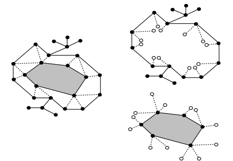
Figure 3: Example for the proof of Lemma 23. The outermost edges in $G$ form its first peeling; the edges enclosing the shaded area form its second peeling; the shaded area, including the nodes of the second peeling, is a subgraph of $G$ of outerplanarity $k$. $G_{1}$ and $G_{2}$ are shown in planar embeddings of outerplanarity $2$ and $k$, respectively. An open edge (dashed line) in $G_{1}$ and $G_{2}$ has a hook (white node) as one of its two endpoints.

$G_{1}$

$G$                                                                              $G_{2}$

We can “re-build” $G$ from $G_{1}$ and $G_{2}$ as follows:

$$V(G)\ =\ \ \bigl{(}V(G_{1})\cup V(G_{2})\bigr{)}\ -\ \bigl{(}\mathsf{hook}_{*}(G_{1})\cup\mathsf{hook}_{*}(G_{2})\bigr{)}$$

$$E(G)\ = E_{c}(G_{1})\ \cup\ E_{c}(G_{2})\ \cup$$

$$\{\,\langle v,w,\ell\rangle\;|\;\langle v,\mathsf{hook}_{\ell}(w),\ell\rangle\in E_{o}(G_{1})\text{ and }\langle\mathsf{hook}_{\ell}(v),w,\ell\rangle\in E_{o}(G_{2})\,\}$$

The preceding are not definitions of $V(G)$ and $E(G)$, but rather equalities that are easily checked against the earlier definitions. They make explicit the way in which we use hooks and open edges to connect two graphs.

Let $G_{1}^{\prime}$ be the graph obtained from $G_{1}$ according to the transformation defined in the lemma statement, which produces a planar embedding of $G_{1}^{\prime}$ with outerplanarity $\leqslant 2$. And let $G_{2}^{\prime}$ be the graph obtained from $G_{2}$ according to the transformation defined in the lemma statement, which, by the induction hypothesis, produces a planar embedding of $G_{2}^{\prime}$ with outerplanarity $\leqslant 2k$.

We note carefully how open edges in $G_{1}$ may get transformed into open edges in $G_{1}^{\prime}$. Consider a vertex $v\in P$ with ${\mathit{deg}}(v)=d\geqslant 4$ and let the open edges of $G_{1}$ that have $v$ as one of their two endpoints be:

$$\langle v,\mathsf{hook}_{\ell_{1}}(w_{1}),\ell_{1}\rangle\ ,\ \ \ldots\ \ ,\ \langle v,\mathsf{hook}_{\ell_{t}}(w_{t}),\ell_{t}\rangle$$

where $1\leqslant t\leqslant d$. The number $t$ of open edges with endpoint $v$ is not necessarily $d$. The corresponding open edges in $G_{1}^{\prime}$ are:

$$\langle v_{i_{1}},\mathsf{hook}_{\ell_{1}}(w_{1}),\ell_{1}\rangle,\ \ldots\ ,\langle v_{i_{t}},\mathsf{hook}_{\ell_{t}}(w_{t}),\ell_{t}\rangle$$

where $\{v_{i_{1}},\ldots,v_{i_{t}}\}\subseteq\{v_{1},\ldots,v_{d}\}$, and $\{v_{1},\ldots,v_{d}\}$ is the set of fresh vertices in the simple cycle that replaces $v$ in $G^{\prime}_{1}$. Note that the transformation from $G_{1}$ to $G^{\prime}_{1}$ does not affect the second endpoints (the hooks) of these open edges, because the degree of a hook is always $=1$. Similar observations apply to the way in which open edges in $G_{2}$ get transformed into open edges in $G_{2}^{\prime}$.

We are ready to define the desired graph $G^{\prime}$ by connecting $G_{1}^{\prime}$ and $G_{2}^{\prime}$ via their hooks and open edges, in the same way in which we can re-connect $G$ from $G_{1}$ and $G_{2}$:

$$V(G^{\prime})\ =\ \ \bigl{(}V(G^{\prime}_{1})\ \ \cup\ V(G^{\prime}_{2})\bigr{)}\ -\ \bigl{(}\mathsf{hook}_{*}(G^{\prime}_{1})\cup\mathsf{hook}_{*}(G^{\prime}_{2})\bigr{)}$$

$$E(G^{\prime})\ = E_{c}(G^{\prime}_{1})\ \ \cup\ E_{c}(G^{\prime}_{2})\ \ \cup$$

$$\{\,\langle v_{i},w_{j},\ell\rangle\; |\;\text{there are $v\in P$ and $w\in Q$ such that}$$

$$\;\;\;\langle v_{i},\mathsf{hook}_{\ell}(w),\ell\rangle\in E_{o}(G^{\prime}_{1})\text{ and }\langle\mathsf{hook}_{\ell}(v),w_{j},\ell\rangle\in E_{o}(G^{\prime}_{2}),$$

$$\;\;\;\text{where $1\leqslant i\leqslant{\mathit{deg}}(v)$ and $1\leqslant j\leqslant{\mathit{deg}}(w)$}\,\}$$

This produces a planar graph $G^{\prime}$ together with a planar embedding. To conclude the induction and the proof, it suffices to note that the outerplanarity of $G^{\prime}$ is “the outerplanarity of $G_{1}$” + “the outerplanarity of $G_{2}$” which is therefore $\leqslant 2k$. ∎

Proof 24 (for Lemma 6).

The computation is a little easier if we introduce a new node $\nu_{\text{in,out}}$ and connect the tail of every input arc $a\in\mathbf{A}_{\text{in}}$ to $\nu_{\text{in,out}}$, i.e., $\text{\em tail}(a)=\nu_{\text{in,out}}$, and the head of every output arc $b\in\mathbf{A}_{\text{out}}$ to $\nu_{\text{in,out}}$, i.e., $\text{\em head}(b)=\nu_{\text{in,out}}$. In the resulting network, there are no input arcs and no output arcs, with $r=n+1$ nodes. The number $m$ of arcs remains unchanged, and they are now all internal arcs. With no loss of generality, we assume for every $\nu\in\mathbf{N}$:

• ${\mathit{deg}}(\nu)\geqslant 3$,

• $\mathsf{in\text{-}degree}(\nu)\neq 0\neq\mathsf{out\text{-}degree}(\nu)$.

It is easy to see that every node $\nu$ violating one of the preceding assumptions can be eliminated from ${\cal N}$. Also, with no loss of generality, assume that $|\,\mathbf{A}_{\text{in}}\,|+|\,\mathbf{A}_{\text{out}}\,|=p+q\geqslant 3$, so that ${\mathit{deg}}(\nu_{\text{in,out}})\geqslant 3$. We also assume:

• the outerplanarity $k$ of ${\cal N}$ is $\geqslant 2$.

The case $k=1$ is handled similarly, with few minor adjustments (which, in fact, makes it easier).

The construction of ${\cal N}^{\prime}$ from ${\cal N}$ proceeds in two parts, with each taking time ${\cal O}(n)$. The first part consists in eliminating all two-node cycles. Let $\gamma$ be a two-node cycle, i.e., there are two arcs $a$ and $a^{\prime}$ such that:

$$\text{\em tail}(a)=\text{\em head}(a^{\prime})=\nu\quad\text{\ and\ }\quad\text{\em head}(a)=\text{\em tail}(a^{\prime})=\nu^{\prime}.$$

To eliminate $\gamma$ as a two-node cycle, we insert a new node $\mu$ in the middle of $a$, another new node $\mu^{\prime}$ in the middle of $a^{\prime}$, and add a new arc $b=\langle\mu,\mu^{\prime}\rangle$. We make the new arc $b$ dummy, by setting $\underline{\bm{c}}(b)=\overline{\bm{c}}(b)=0$, which prevents it from carrying any flow. Clearly:

• ${\mathit{deg}}(\mu)={\mathit{deg}}(\mu^{\prime})=3$.

• If the two arcs $a$ and $a^{\prime}$ do not enclose an inner face of ${\cal N}$, one of the two can be redrawn so that after inserting the new arc $b$, planarity is preserved.

• If $k\geqslant 2$, it is easy to see that the outerplanarity remains the same. (This is the reason for assumption (3).)

This operation can be extended to all two-node cycles in ${\cal N}$ in time ${\cal O}(n)$, resulting in an equivalent network, with fewer than $m$ new nodes and fewer than $\lceil m/2\rceil$ new arcs, and where the degree of every node $\geqslant 3$.

The second part of the construction consists in replacing every node $\nu\in\mathbf{N}$ with ${\mathit{deg}}(\nu)=s\geqslant 4$ by an appropriate cycle with $s$ new nodes, say $\{\nu_{1},\ldots,\nu_{s}\}$, to obtain a network satisfying conclusions 2, 3, 4, and 5. More specifically, consider the arcs incident to $\nu$, say:

$$\{a_{1},\ldots,a_{s}\}\ :=\ \{\,a\in\mathbf{A}\;|\;\text{\em head}(a)=\nu\text{ or }\text{\em tail}(a)=\nu\,\}.$$

We introduce $s$ new arcs, say $\{b_{1},\ldots,b_{s}\}$, to form a directed cycle connecting the new nodes $\{\nu_{1},\ldots,\nu_{s}\}$. We make each new node $\nu_{i}$ the endpoint of an arc in $\{a_{1},\ldots,a_{s}\}$, i.e., for every $1\leqslant i\leqslant s$:

• if $\text{\em head}(a_{i})=\nu$, we set $\text{\em head}(a_{i}):=\nu_{i}$,

• if $\text{\em tail}(a_{i})=\nu$, we set $\text{\em tail}(a_{i}):=\nu_{i}$.

An example of the transformation from the node $\nu$ to the directed cycle replacing it is shown in Figure 4.

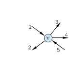
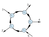
Figure 4: A node $\nu$ of degree $=5$ (on the left) is transformed into a cycle with $5$ nodes $\nu_{1},\nu_{2},\nu_{3},\nu_{4},$ and $\nu_{5}$, (on the right), each of degree $=3$. The transformation preserves planarity.

We want the cycle connecting the new nodes $\{\nu_{1},\ldots,\nu_{s}\}$ to put no restriction on flows, so we set all the lower bounds to $0$ and all the upper bounds to the “very large number” $K$:

$$\underline{\bm{c}}(b_{1}):=\cdots:=\underline{\bm{c}}(b_{s}):=0\quad\text{ and }\quad\overline{\bm{c}}(b_{1}):=\cdots:=\overline{\bm{c}}(b_{s}):=K.$$

Repeating the preceding operation for every node $\nu\in\mathbf{N}$, it is straightforward to check that conclusions 1, 2, and 3, in the statement of Lemma 6 are satisfied, and the construction can be carried out in time ${\cal O}(n)$.

For conclusion 4, consider an arc $a\in\mathbf{A}$. If $a$ is incident to one node $\nu$ of degree $\geqslant 4$ (resp. two nodes $\nu$ and $\mu$ of degree $\geqslant 4$), then the preceding construction introduces one new arc corresponding to $a$ in the cycle simulating $\nu$ in ${\cal N}^{\prime}$ (resp. two new arcs corresponding to $a$, one in the cycle simulating $\nu$ and one in the cycle simulating $\mu$, in ${\cal N}^{\prime}$). Hence, the number $m^{\prime}$ of arcs in ${\cal N}^{\prime}$ is such that $m^{\prime}\leqslant 3m$.

Moreover, because every arc is incident to two distinct nodes and for every node $\nu$ in ${\cal N}^{\prime}$ there are exactly three arcs incident to $\nu$, the number $n^{\prime}$ of nodes in ${\cal N}^{\prime}$ is such that $n^{\prime}=2m^{\prime}/3\leqslant 2m$.

It remains to prove conlusion 5. The preceding construction preserves planarity: If ${\cal N}$ is given with a planar embedding, the new ${\cal N}^{\prime}$ is produced with a planar embedding.

The standard notion of an undirected graph $G$ does not include the presence of one-ended edges corresponding to input/output arcs in a network ${\cal N}$. In order to turn the input/output arcs of network ${\cal N}$ into two-ended edges in graph $G$ we simply add a new node of degree $=1$ at the end of every input/output arc missing a node.

With the preceding qualification, we can take $G$ to be the undirected simple graph corresponding to network ${\cal N}$ after elimination of all two-node directed cycles. This is the first part in the two-part construction of ${\cal N}^{\prime}$ from ${\cal N}$. Absence of two-node cycles allows us to take $G$ as a simple graph (no multiple edges). Every vertex in $G$ has thus degree $1$ or degree $\geqslant 3$, as we assume that all nodes in ${\cal N}$ have degrees $\geqslant 3$.

We take $G^{\prime}$ to be the undirected simple graph corresponding to network ${\cal N}^{\prime}$ after the second part in the construction. The construction of $G^{\prime}$ from $G$ in Lemma 23 corresponds to the construction of ${\cal N}^{\prime}$ from ${\cal N}$ after elimination of all two-node cycles. The conclusion of Lemma 23 implies conclusion 5 in Lemma 6. $\square$

Example 25.

Consider the planar network ${\cal N}$ on the left in Figure 5. We transform ${\cal N}$ into a $3$-regular network ${\cal N}^{\prime}$ according to the construction in the proof of Lemma 6. We omit all arc directions in ${\cal N}$ which play no role in the transformation.

The outerplanarity of ${\cal N}$ is $3$: There are three enclosing peelings (drawn with foldface arcs on the left in Figure 5). The outerplanarity of ${\cal N}^{\prime}$ is guaranteed not to exceed $6$ by Lemma 23, but is also $3$ in this example, as one can easily check.

On the right in Figure 6, ${\cal N}^{\prime}$ is re-drawn on a rectangular grid – except for two arcs because of a missing north-east corner and a missing south-west corner – which makes its outerplanarity ($=3$) explicit and reasoning in the proof of Theorem 5 easier to follow. This re-drawing can always be done in linear time [42]. $\square$

Assumption 26.

From now on, there is no loss of generality if we assume that:

1. Networks are connected.

2. Networks are $3$-regular.

3. There are no two-node cycles in networks.

4. No two distinct input/output arcs are incident to the same node.

The second and third conditions follow from the construction in the proof of Lemma 6. The fourth condition is equivalent to saying that a node cannot be both a source and a sink. $\square$

The next definition, and lemma based on it, are not essential. But, together with the preceding assumption, they simplify considerably Algorithm 4 and proving its correctness.

Definition 27 (Good Planar Embeddings).

Let ${\cal N}=(\mathbf{N},\mathbf{A})$ be a network satisfying Assumption 26 and given in a fixed $k$-outerplanar embedding, for some $k\geqslant 1$. From the peelings $L_{1},\ldots,L_{k}$ specified in Definition 22, we define the sets of nodes $L^{\prime}_{1},\ldots,L^{\prime}_{k}$, respectively, as follows. For every $1\leqslant i\leqslant k$:

$$L_{i}^{\prime}:=L_{i}-\{\,\nu\in L_{i}\;|\;\text{$\nu$ is incident to at most one peeling arc}\,\}.$$

In words, $L_{i}^{\prime}$ is a subset of $L_{i}$ which is proper whenever $L_{i}$ contains a node $\nu$ such that:

1. $\nu$ is incident to three cross arcs.

2. $\nu$ is incident to two cross arcs and one input/output arc.

3. $\nu$ is incident to one cross arc and one input/output arc.

Thus, $L_{i}^{\prime}$ is defined to exclude all the nodes of $L_{i}$ that are of degree $\leqslant 1$ in the network ${\cal N}_{i}$ (see Definition 22).

We say the planar embedding of ${\cal N}$ is good if for every $1\leqslant i\leqslant k$, the nodes in $L_{i}^{\prime}$ form a single (undirected) simple cycle, namely, the outermost one, in the network ${\cal N}_{i}$. $\square$

Example 28.

For an example of how $L_{i}^{\prime}$ may be different from $L_{i}$, consider the $3$-outerplanar embedding in Figure 6: $L_{1}=L_{1}^{\prime}$ and $L_{3}=L_{3}^{\prime}$, but $L_{2}\neq L_{2}^{\prime}$. The latter inequality is caused by one of the nodes on the periphery of the south-east face, which is incident to one cross arc and one input/output arc.

In a good planar embedding, the sets $L^{\prime}_{1},\ldots,L^{\prime}_{k}$ can be viewed as forming $k$ concentric simple cycles. All the nodes in $(L_{i}-L_{i}^{\prime})$ occur between the level-$i$ concentric cycle and the one immediately enclosing it (the level-$(i-1)$ concentric cycle). This implies that, if ${\cal N}$ is $3$-regular and no two distinct input/output arcs are incident to the same node (as required by Assumption 26), then $L_{1}=L_{1}^{\prime}$ but we may have $L_{i}\neq L_{i}^{\prime}$ for $i\geqslant 2$. The $3$-outerplanar embedding in Figure 6 is good. $\square$

Lemma 29 (From Planar Embeddings to Good Planar Embeddings).

Let ${\cal N}=(\mathbf{N},\mathbf{A})$ be a network satisfying Assumption 26 and given in a specific planar embedding. In time ${\cal O}(n)$, where $n=|\,\mathbf{N}\,|$, we can transform the given planar embedding of ${\cal N}$ into a planar embedding of an equivalent ${\cal N}^{\prime}=(\mathbf{N}^{\prime},\mathbf{A}^{\prime})$ such that:

1. The planar embedding of ${\cal N}^{\prime}$ is good (and, in particular, ${\cal N}^{\prime}$ satisfies Assumption 26).

2. $|\,\mathbf{N}^{\prime}\,|\leqslant 2\cdot|\,\mathbf{N}\,|$ and $|\,\mathbf{A}^{\prime}\,|\leqslant 2\cdot|\,\mathbf{A}\,|$.

3. ${\cal N}$ and ${\cal N}^{\prime}$ have the same outerplanarity.

Proof.

Straightforward, by appropriately inserting dummy arcs, also making sure not to violate $3$-regularity and not to increase outerplanarity. An arc $a$ is dummy arc if $\underline{\bm{c}}(a)=\overline{\bm{c}}(a)=0$, i.e., $a$ cannot carry any flow and therefore cannot affect the overall flow properties of the network. ∎

Lemma 30 (Paths of Nodes in $(L_{i}-L_{i}^{\prime})$).

Let network ${\cal N}$ be given in a good $k$-outerplanar embedding, for some $k\geqslant 1$, which satisfies in particular Assumption 26. Suppose $(L_{i}-L_{i}^{\prime})\neq\varnothing$ for some $1\leqslant i\leqslant k$ and consider a maximal-length undirected path $\langle\nu_{0},\nu_{1},\ldots,\nu_{p-1}\rangle$ formed by node $\nu_{0}\in L_{i}^{\prime}$ and nodes $\{\nu_{1},\ldots,\nu_{p-1}\}\subseteq(L_{i}-L_{i}^{\prime})$ for some $p\geqslant 2$.

Conclusion: There is a node $\nu_{p}\in L^{\prime}_{i-1}$, together with $(p-1)$ level-$i$ peeling arcs $\{a_{1},\ldots,a_{p-1}\}$, one cross arc $a_{p}$, and $(p-1)$ input/output arcs $\{b_{1},\ldots,b_{p-1}\}$ of ${\cal N}$, such that:

1. $\{\text{\em head}(a_{1}),\text{\em tail}(a_{1})\}=\{\nu_{0},\nu_{1}\},\ \ldots\ ,\{\text{\em head}(a_{p-1}),\text{\em tail}(a_{p-1})\}=\{\nu_{p-2},\nu_{p-1}\}$
   and $\{\text{\em head}(a_{p}),\text{\em tail}(a_{p})\}=\{\nu_{p-1},\nu_{p}\}$.

2. For every $1\leqslant j\leqslant p-1$, either $\text{\em head}(b_{j})$ is defined and $\text{\em head}(b_{j})=\nu_{j}$ or $\text{\em tail}(b_{j})$ is defined and $\text{\em tail}(b_{j})=\nu_{j}$.

In words, the undirected path $\langle\nu_{0},\nu_{1},\ldots,\nu_{p-1},\nu_{p}\rangle$, which is the same as $\langle a_{1},\ldots,a_{p}\rangle$ as a sequence of internal arcs, connects node $\nu_{0}\in L_{i}^{\prime}$ and node $\nu_{p}\in L^{\prime}_{i-1}$, with $(p-1)$ input/output arcs incident to the $(p-1)$ intermediate nodes along this path.

Proof.

Straightforward from the definitions. All details omitted. ∎

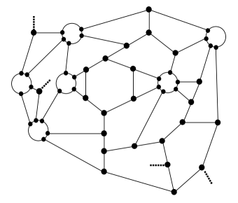
Figure 5: Example of a planar network ${\cal N}$ (with all arc directions ignored) on the left, its transformation into a 3-regular network ${\cal N}^{\prime}$ according to Lemma 6 on the right. The dashed arcs are input/output arcs, $4$ of them.

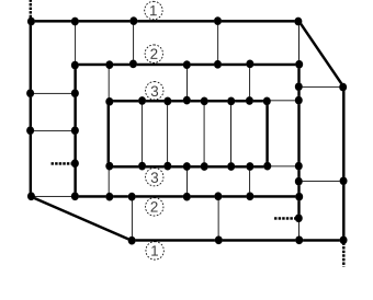
Figure 6: The planar network ${\cal N}^{\prime}$ on the right in Figure 5 is reproduced without change on the left in this figure, and re-drawn on a rectangular grid on the right in this figure – except for two arcs because of the missing north-east corner and south-west corner. The dashed arcs are input/output arcs, $4$ of them.

Remark 31.

In Section 4 and Appendix B, where we had to worry about finding typings of subnetworks of the given network ${\cal N}=(\mathbf{N},\mathbf{A})$, the same arc $a\in\mathbf{A}$ could be an input arc in a subnetwork ${\cal M}^{\prime}$ and an output arc in another subnetwork ${\cal M}^{\prime\prime}$, in which case we temporarily re-named it $a^{+}$ in ${\cal M}^{\prime}$ and $a^{-}$ in ${\cal M}^{\prime\prime}$. In this appendix, there is no issue about computing typings and we can do away with this distinction between “$a$ as input arc” and “$a$ as output arc” in two distinct subnetworks.

Moreover, whenever convenient, we ignore arc directions. Our concern is to minimize the number of interface links, as we break up and re-assemble networks, and this is not affected by arc directions. $\square$

Recall the definitions of “subnetwork” and “component” of a network ${\cal N}$ in Section 3, which mimic the standard defnitions of “subgraph” and “component” except for the presence of input/output arcs. For a precise statement of Algorithm 4, we need the notions of “neighbor subnetworks” and how to “merge” them.

Definition 32 (Neighbor Subnetworks and their Merge).

Let ${\cal N}=(\mathbf{N},\mathbf{A})$ be a network, and consider two non-empty disjoint subsets of nodes: $X,X^{\prime}\subseteq\mathbf{N}$ with $X\cap X^{\prime}=\varnothing$. Let ${\cal M}$ and ${\cal M}^{\prime}$ be the subnetworks of ${\cal N}$ induced by $X$ and $X^{\prime}$, respectively. Let $\mathbf{B}_{\text{in,out}}$ and $\mathbf{B}^{\prime}_{\text{in,out}}$ be the input/output arcs of ${\cal M}$ and ${\cal M}^{\prime}$. We say ${\cal M}$ and ${\cal M}^{\prime}$ are neighbor subnetworks, or just neighbors, iff $|\,\mathbf{B}_{\text{in,out}}\cap\mathbf{B}^{\prime}_{\text{in,out}}\,|\geqslant 1$, i.e., ${\cal M}$ and ${\cal M}^{\prime}$ have one input/output arc or more in common. We refer to the sequence of arcs in $\mathbf{B}_{\text{in,out}}\cap\mathbf{B}^{\prime}_{\text{in,out}}$ listed according to some fixed (but otherwise arbitrary) ordering scheme as the sequence of joint arcs of ${\cal M}$ and ${\cal M}^{\prime}$:

$$\mathsf{joint\text{-}arcs}({\cal M},{\cal M}^{\prime})\ :=\ \text{a fixed ordering of the arcs in $\mathbf{B}_{\text{in,out}}\cap\mathbf{B}^{\prime}_{\text{in,out}}$}.$$

Observe that we restrict the notion of “neighbors” to two subnetworks ${\cal M}$ and ${\cal M}^{\prime}$ induced by disjoint subsets of nodes $X$ and $X^{\prime}$, but which share some input/output arcs.

To merge ${\cal M}$ and ${\cal M}^{\prime}$ means to produce the subnetwork of ${\cal N}$ induced by $X\cup X^{\prime}$, which we denote $({\cal M}{\otimes}{\cal M}^{\prime})$. If ${\cal M}$ and ${\cal M}^{\prime}$ are not neighbors, then $({\cal M}{\otimes}{\cal M}^{\prime})$ is undefined. $\square$

Definition 33 (Strong Neighbors).

Let ${\cal N}=(\mathbf{N},\mathbf{A})$ be a network, and ${\cal M}^{\prime}$ and ${\cal M}^{\prime\prime}$ be neighbors in ${\cal N}$ induced by the disjoint subsets of nodes $X^{\prime}$ and $X^{\prime\prime}$, as in Definition 32. We define the binding strength of the neighbors ${\cal M}^{\prime}$ and ${\cal M}^{\prime\prime}$ as follows:

$$\mathsf{binding\text{-}strength}({\cal M}^{\prime},{\cal M}^{\prime\prime})\ :=\ \ |\,\mathsf{joint\text{-}arcs}({\cal M}^{\prime},{\cal M}^{\prime\prime})\,|.$$

Because ${\cal M}^{\prime}$ and ${\cal M}^{\prime\prime}$ are neighbors, $\mathsf{binding\text{-}strength}({\cal M}^{\prime},{\cal M}^{\prime\prime})\geqslant 1$. The external dimension of ${\cal M}^{\prime}{\otimes}{\cal M}^{\prime\prime}$ is:

$$\mathsf{exDim}({\cal M}^{\prime}{\otimes}{\cal M}^{\prime\prime})\ =\ \mathsf{exDim}({\cal M}^{\prime})+\mathsf{exDim}({\cal M}^{\prime\prime})-2\cdot\mathsf{binding\text{-}strength}({\cal M}^{\prime},{\cal M}^{\prime\prime}).$$

We say ${\cal M}^{\prime}$ and ${\cal M}^{\prime\prime}$ are strong neighbors if the following inequality is satisfied:

$$\mathsf{exDim}({\cal M}^{\prime}{\otimes}{\cal M}^{\prime\prime})\ \leqslant$$

$$\min\;\bigl{(}\{\,\mathsf{exDim}({\cal M}^{\prime}{\otimes}{\cal M})\;|\;\text{${\cal M}$ is a neighbor of ${\cal M}^{\prime}$}\,\}$$

$$\qquad\ \ \ \cup\{\,\mathsf{exDim}({\cal M}^{\prime\prime}{\otimes}{\cal M})\;|\;\text{${\cal M}$ is a neighbor of ${\cal M}^{\prime\prime}$}\,\}\bigr{)}.$$

Equivalently, ${\cal M}^{\prime}$ and ${\cal M}^{\prime\prime}$ are strong neighbors if:

$$\mathsf{binding\text{-}strength}({\cal M}^{\prime},{\cal M}^{\prime\prime})\ \geqslant$$

$$\max\;\bigl{(}\{\,\mathsf{binding\text{-}strength}({\cal M}^{\prime},{\cal M})\;|\;\text{${\cal M}$ is a neighbor of ${\cal M}^{\prime}$}\,\}$$

$$\qquad\ \ \ \cup\{\,\mathsf{binding\text{-}strength}({\cal M}^{\prime\prime},{\cal M})\;|\;\text{${\cal M}$ is a neighbor of ${\cal M}^{\prime\prime}$}\,\}\bigr{)}.$$

In words, ${\cal M}^{\prime}$ and ${\cal M}^{\prime\prime}$ are strong neighbors if they have at least as many external arcs in common as each has in common with another neighbor ${\cal M}$. $\square$

In Algorithm 4, we use repeatedly the same group of instructions, which we here collect together as a single “macro” instruction called $\mathsf{Merge}$. Let $X_{1}\uplus\cdots\uplus X_{p}=\mathbf{N}$ be a partition of the nodes of the given network ${\cal N}$. Let $\mathscr{C}=\{{\cal M}_{1},\ldots,{\cal M}_{p}\}$ be the subnetworks of ${\cal N}$ induced by $X_{1},\ldots,X_{p}$, respectively. Let $\mathbf{B}_{\text{\#}}^{1},\ldots,\mathbf{B}_{\text{\#}}^{p}$ be the (necessarily disjoint) sets of internal arcs of ${\cal M}_{1},\ldots,{\cal M}_{p}$, respectively. With ${\cal N}$ thus disassembled, if we select two distinct subnetworks ${\cal M},{\cal M}^{\prime}\in\mathscr{C}$ that are neighbors, we write $\mathsf{Merge}$ with $5$ arguments as:

$$\mathsf{Merge}({\cal M},{\cal M}^{\prime},\sigma,\delta,\mathscr{C})$$

where the last $3$ are the following quantities:

• $\sigma=\text{an ordering of the arcs in $\mathbf{B}_{\text{\#}}^{1}\cup\cdots\cup\mathbf{B}_{\text{\#}}^{p}$}$   (the binding schedule computed by the algorithm)

• $\delta\geqslant 3$   (a tight upper bound on ${\mathit{index}}(\sigma)$)

• $\mathscr{C}=\{{\cal M}_{1},\ldots,{\cal M}_{p}\}$

The notions of a “binding schedule” and its “index” were defined in Section 4. The macro expansion of $\mathsf{Merge}({\cal M},{\cal M}^{\prime},\sigma,\delta,\mathscr{C})$ is shown in Figure 7.

$\displaystyle 1.\quad$ $\displaystyle\sigma\$ $\displaystyle:=\ \$ $\displaystyle\sigma\ \;\mathsf{joint\text{-}arcs}({\cal M},{\cal M}^{\prime})\quad$ // append $\mathsf{joint\text{-}arcs}({\cal M},{\cal M}^{\prime})$ to $\sigma$ $\displaystyle 2.$ $\displaystyle\delta\$ $\displaystyle:=\$ $\displaystyle\max\{\delta,\;\mathsf{exDim}({\cal M})+\mathsf{exDim}({\cal M}^{\prime})-2\}\quad$ // new tight upper bound on ${\mathit{index}}(\sigma)$ $\displaystyle 3.$ $\displaystyle\mathscr{C}\$ $\displaystyle:=\$ $\displaystyle(\mathscr{C}-\{{\cal M},{\cal M}^{\prime}\})\cup\{{\cal M}{\otimes}{\cal M}^{\prime}\}\quad$ // exclude ${\cal M}$ and ${\cal M}^{\prime}$, include their merge ${\cal M}{\otimes}{\cal M}^{\prime}$

Figure 7: Macro expansion of $\mathsf{Merge}({\cal M},{\cal M}^{\prime},\sigma,\delta,\mathscr{C})$.

Instead of the three instructions shown in Figure 7, we can now write a single macro instruction:

$$(\sigma,\,\delta,\,\mathscr{C})\ :=\ \mathsf{Merge}({\cal M},{\cal M}^{\prime},\sigma,\delta,\mathscr{C})$$

We need one more classification of arcs before we define Algorithm 4. Let network ${\cal N}=(\mathbf{N},\mathbf{A})$ be given in a good $k$-outerplanar embedding, with $\mathbf{A}=\mathbf{A}_{\text{in,out}}\uplus\mathbf{A}_{\text{\#}}$. Using Lemma 30, we partition the internal arcs of ${\cal N}$ into two parts, $\mathbf{A}_{\text{\#}}=\mathbf{A}_{\text{\#,1}}\uplus\mathbf{A}_{\text{\#,2}}$, where:

$$\mathbf{A}_{\text{\#,1}}\ :=\ \bigl{\{}\,a\in\mathbf{A}_{\text{\#}}\;|\;\text{$a$ is a cross arc}\,\bigr{\}}\ \cup$$

$$\bigl{\{}\,a\in\mathbf{A}_{\text{\#}}\;|\;\text{there is $1\leqslant i\leqslant k$ such that such that $\{\text{\em head}(a),\text{\em tail}(a)\}\cap(L_{i}-L_{i}^{\prime})\neq\varnothing$}\,\bigr{\}},$$

$$\mathbf{A}_{\text{\#,2}}\ :=\ \mathbf{A}_{\text{\#}}-\mathbf{A}_{\text{\#,1}}.$$

In words, $\mathbf{A}_{\text{\#,1}}$ is the set of: (1) all cross arcs, and (2) all peeling arcs on a path connecting two consecutive concentric cycles of the good embedding of ${\cal N}$. See the statement of Lemma 30 for further explanation.

Algorithm 4  $\mathsf{BindSchedule}$: Define Optimal Binding Schedule

1:input: good planar embedding of network ${\cal N}=(\mathbf{N},\mathbf{A})$, with $\mathbf{A}=\mathbf{A}_{\text{in,out}}\uplus\mathbf{A}_{\text{\#,1}}\uplus\mathbf{A}_{\text{\#,2}}$

2:output: $\sigma=b_{1}b_{2}\cdots b_{m}$, an ordering of internal arcs of ${\cal N}$ (a “binding schedule”),

3:           where  $\mathbf{A}_{\text{\#}}=\{b_{1},b_{2},\ldots,b_{m}\}$, together with a tight upper bound $\delta$ on ${\mathit{index}}(\sigma)$.

4: 

5:initialization

6:$k:=\ \text{outerplanarity of ${\cal N}$}$

7:$\sigma:=\ \varepsilon$         // $\sigma$ is initially the empty “binding schedule”

8:$\mathscr{C}:=\ \bigl{\{}\,{\cal M}\;\bigl{|}\;\text{${\cal M}$ subnetwork of ${\cal N}$ induced by $\{\nu\}$ with $\nu\in\mathbf{N}$}\,\bigr{\}}$

9:                 // ${\cal N}$ is disassembled into $|\,{\cal N}\,|$ one-node subnetworks, each of external dimension $3$

10:first iteration   // pre-processing

11:for every arc $a\in\mathbf{A}_{\text{\#,1}}$ do

12:     $(\sigma,\delta,\mathscr{C}):=\ \mathsf{Merge}({\cal M},{\cal M}^{\prime},\sigma,\delta,\mathscr{C})$

13:  where ${\cal M},{\cal M}^{\prime}\in\mathscr{C}$ are the two subnetworks such that $a\in\mathsf{joint\text{-}arcs}({\cal M},{\cal M}^{\prime})$

14:end for  // every arc $a\in\mathbf{A}_{\text{\#,1}}$ is now included in $\sigma$,

15:     // for every ${\cal M}\in\mathscr{C}$ such that $|\,{\cal M}\,|=1$, the single node of ${\cal M}$ is an input/output node,

16:     // for every ${\cal M}\in\mathscr{C}$ such that $|\,{\cal M}\,|\geqslant 2$, ignoring input/output arcs of ${\cal N}$, $\mathsf{exDim}({\cal M})=4$

17:second iteration   // pre-processing

18:while there are neighbors ${\cal M},{\cal M}^{\prime}\in\mathscr{C}$ such that: $|\,{\cal M}\,|=1$  or $\mathsf{binding\text{-}strength}({\cal M},{\cal M}^{\prime})=2$  do

19:     $(\sigma,\delta,\mathscr{C}):=\ \mathsf{Merge}({\cal M},{\cal M}^{\prime},\sigma,\delta,\mathscr{C})$

20:end while  // for every ${\cal M}\in\mathscr{C}$, ignoring input/output arcs of ${\cal N}$, $\mathsf{exDim}({\cal M})=4$

21:main iteration   // re-assemble ${\cal N}$ from the subnetworks in $\mathscr{C}$ and store it in ${\cal P}$

22: ${\cal P}:=\ {\cal M}$ where ${\cal M}$ is any “outermost” subnetwork in $\mathscr{C}$

23:$\mathscr{C}:=\ \mathscr{C}-\{{\cal P}\}$

24:while $\mathscr{C}\neq\varnothing$ do

25:      select ${\cal M}\in\mathscr{C}$ which is a strong neighbor of ${\cal P}$

26:     $\sigma:=\ \sigma\ \;\mathsf{joint\text{-}arcs}({\cal P},{\cal M})$

27:     $\delta:=\ \max\{\delta,\;\mathsf{dim}({\cal P})+\mathsf{dim}({\cal M})-2\}$

28:     ${\cal P}:={\cal P}{\otimes}{\cal M}$

29:     $\mathscr{C}:=\mathscr{C}-\{{\cal M}\}$

30:end while  // ${\cal N}$ is now re-assembled and stored in ${\cal P}$

31:return $\sigma$ and $\delta$

Example 34.

This is a continuation of the network considered in Examples 25 and 28. They refer to the good $3$-outerplanar embedding on the right in Figure 5, and again in Figure 6, which we use to illustrate the operation of Algorithm 4. The progress of Algorithm 4 is shown in Figure 8, for the first iteration and the second iteration, and in Figure 9 for the main iteration. $\square$

Proof 35 (for Theorem 5).

Let ${\cal N}_{0}$ be the network ${\cal N}$ in the statement of Theorem 5, to distinguish it from the “${\cal N}$” introduced below. Let ${\cal N}_{0}=(\mathbf{N}_{0},\mathbf{A}_{0})$ be given in a $k_{0}$-outerplanar embedding, for some $k_{0}\geqslant 1$. Let $p=|\,\mathbf{A}_{0,\text{in}}\,|\geqslant 1$, $q=|\,\mathbf{A}_{0,\text{out}}\,|\geqslant 1$, $m_{0}=|\,\mathbf{A}_{0,\text{\#}}\,|\geqslant 1$ and $n_{0}=|\,\mathbf{N}_{0}\,|\geqslant 1$. Because ${\cal N}_{0}$ is planar, ${\cal N}_{0}$ is sparse; more specifically, $m_{0}\leqslant 3n_{0}-6$ (see, for example, Theorem 4.2.7 and its corollaries in [18]). Hence, the complexity bound ${\cal O}(m_{0}+n_{0})$ is the same as ${\cal O}(n_{0})$.

By Lemmas 6 and 29, we can transform the $k_{0}$-outerplanar embedding of ${\cal N}_{0}$ into a good $k$-outerplanar embedding of an equivalent ${\cal N}$, with $k\leqslant 2k_{0}$. The transformation is such that $\mathsf{exDim}({\cal N}_{0})=\mathsf{exDim}({\cal N})=p+q$. Let $m=|\,\mathbf{A}_{\text{\#}}\,|$ and $n=|\,\mathbf{N}\,|$. By Lemma 6, $m\leqslant 3m_{0}+{\cal O}(m_{0})$ and $n\leqslant 2m_{0}+{\cal O}(m_{0})$, where “${\cal O}(m_{0})$” accounts for the arcs and nodes introduced in the construction of Lemma 29.

We next run Algorithm 4 on the good $k$-outerplanar embedding of ${\cal N}$. We first consider the correctness of the algorithm, and then its run-time complexity. The initialization consists in breaking up ${\cal N}$ into $n$ one-node subnetworks, each of external dimension $=3$.

The first iteration assembles new subnetworks ${\cal M}$ of external dimension $=4$, if we ignore the presence of all input/output arcs of ${\cal N}$. See Figure 8 for an illustration. Such a subnetwork ${\cal M}$ of external dimension $=4$ has two nodes – say $\{\nu_{1},\nu_{2}\}$ – that are either on the same peeling level or on two consecutive peeling levels. Specifically, there is $1\leqslant i\leqslant k$, such that either both $\nu_{1},\nu_{2}\in L_{i}^{\prime}$ or $\nu_{1}\in L_{i}^{\prime}$ and $\nu_{2}\in L_{i+1}^{\prime}$.

A similar conclusion applies to the second iteration: It assembles new subnetworks ${\cal M}$ of external dimension $=4$, again ignoring the presence of all input/output arcs of ${\cal N}$. See Figure 8 for an illustration. Such a subnetwork has external dimension $=4$, with four input/output nodes (these are not the same as the input/output nodes of ${\cal N}$) – say $\{\nu_{1},\nu_{2},\nu_{3},\nu_{4}\}$ – that are either all on the same peeling level or on two consecutive peeling levels with two nodes on each. Specifically, there is $1\leqslant i\leqslant k$, such that either both $\{\nu_{1},\nu_{2},\nu_{3},\nu_{4}\}\subseteq L_{i}^{\prime}$ or $\{\nu_{1},\nu_{2}\}\subseteq L_{i}^{\prime}$ and $\{\nu_{3},\nu_{4}\}\subseteq L_{i+1}^{\prime}$.

At the end of the second iteration, if we ignore all input/output arcs of ${\cal N}$, every subnetwork ${\cal M}$ in $\mathscr{C}$ has external dimension $=4$ and is one of two kinds:

• ${\cal M}$ is assembled in the first iteration and not affected by the second iteration. In this case, ${\cal M}$ straddles either two opposite nodes of the same level $L_{i}^{\prime}$ or two nodes of two consecutive levels $L_{i}^{\prime}$ and $L_{i+1}^{\prime}$.

• ${\cal M}$ is assembled in the second iteration from two or more networks of the previous kind. In this case, ${\cal M}$ straddles either two opposite peeling arcs on the same level or two peeling arcs on two consecutive levels.

At the end of the second iteration, for any two subnetworks ${\cal M}_{1},{\cal M}_{2}\in\mathscr{C}$, if ${\cal M}_{1}$ and ${\cal M}_{2}$ are neighbors, then $\mathsf{binding\text{-}strength}({\cal M}_{1},{\cal M}_{2})=1$.

The task of the main iteration in Algorithm 4 is to re-assemble the original ${\cal N}$ from the subnetworks in $\mathscr{C}$ at the end of the second iteration in such a way as to minimize the external dimension of the intermediate subnetwork ${\cal P}$. We initialize ${\cal P}$ by selecting for it an “outermost” ${\cal M}$ in $\mathscr{C}$ (line 22 of Algorithm 4), i.e., we choose ${\cal M}$ so that all its nodes are either all on level $L_{1}^{\prime}$ or on two consecutive levels $L_{1}^{\prime}$ and $L_{2}^{\prime}$.

The selection of the initial ${\cal M}$ in the main iteration is totally arbitrary. For example, in the third assembly on the right of Figure 8, we choose for this initial ${\cal M}$ the subnetwork containing the north-west corner of ${\cal N}$, and the corresponding progress of Algorithm 4 during the main iteration is shown in Figure 9.

To minimize the external dimension of ${\cal P}$ at every turn of the main iteration, it suffices to select any ${\cal M}\in\mathscr{C}$ which is a strong neighbor of ${\cal P}$ (line 25 of Algorithm 4). For every ${\cal M}\in\mathscr{C}$ which is a neighbor of ${\cal P}$, we have $\mathsf{binding\text{-}strength}({\cal P},{\cal M})\geqslant 1$. Initially, $\mathsf{exDim}({\cal P})=4$ (ignoring all input/output arcs of ${\cal N}$), and the maximum number of strong neighbors ${\cal M}\in\mathscr{C}$ such that $\mathsf{binding\text{-}strength}({\cal P},{\cal M})=1$ in consecutive turns of the main iteration is $(k-1)$. It is now easy to see that $\mathsf{exDim}({\cal P})\leqslant 2k+2$ is an invariant of the main iteration. Figure 9 shows how ${\cal P}$ may be assembled during the main iteration. For a schematic example, which is also easier to follow by making the peeling levels $L_{1}^{\prime},L_{2}^{\prime},L_{3}^{\prime},\ldots$ drawn as concentric ellipses, see Figures 10 and 11.

Consider now a subnetwork ${\cal M}$ which is obtained by merging subnetworks ${\cal M}^{\prime}$ and ${\cal M}^{\prime\prime}$, i.e., ${\cal M}={\cal M}^{\prime}{\otimes}{\cal M}^{\prime\prime}$, where:

• $\mathsf{exDim}({\cal M}^{\prime})=\ell^{\prime}\geqslant 2$ and $\mathsf{exDim}({\cal M}^{\prime\prime})=\ell^{\prime\prime}\geqslant 2$,

• $\mathsf{joint\text{-}arcs}({\cal M}^{\prime},{\cal M}^{\prime\prime})=\{a_{1},\ldots,a_{j}\}$ where $j\leqslant\min\{\ell^{\prime},\ell^{\prime\prime}\}$.

The arcs in $\{a_{1},\ldots,a_{j}\}$ are re-connected one at a time, so that, starting from $\{{\cal M}^{\prime},{\cal M}^{\prime\prime}\}$ and ending with ${\cal M}$, the merge operation produces $j$ intermediate subnetworks (including ${\cal M}$) with external dimensions:

$$(\ell^{\prime}+\ell^{\prime\prime}-2),\ (\ell^{\prime}+\ell^{\prime\prime}-4),\ \ldots\ ,\ (\ell^{\prime}+\ell^{\prime\prime}-2j),$$

respectively. Hence, while $\mathsf{exDim}({\cal P})\leqslant 2k+2$, the maximum external dimension encountered in the course of the operation of Algorithm 4 is – again ignoring all input/output arcs of ${\cal N}$:

$$\text{``maximum external dimension of ${\cal P}$''}+\text{``external dimension of all subnetworks in $\mathscr{C}$''}-2$$

$$\leqslant\ (2k+2)+4-2\ =\ 2k+4,$$

Hence, if we include the presence of the $p+q$ input/output arcs of ${\cal N}$, the maximum external dimension of subnetworks produced during the entire operation of Algorithm 4 cannot exceed $2k+4+p+q$, which is precisely the final value assigned to $\delta$ by Algorithm 4, which is also $\leqslant 4k_{0}+4+p+q$ where $k_{0}$ is the outerplanarity of the original network ${\cal N}_{0}$.

To conclude the proof of Theorem 5, we need to show that the run-time complexity is ${\cal O}(n_{0})={\cal O}(n)$. This is a straightforward consequence of the fact that:

1. The initial transformation from ${\cal N}_{0}$ to ${\cal N}$ is carried out in time ${\cal O}(n_{0})$, according to Lemmas 6 and 29.

2. Each of the four stages in Algorithm 4 (initialization, first iteration, second iteration, and main iteration) runs in time ${\cal O}(m)$, which is the same as ${\cal O}(m_{0})={\cal O}(n_{0})$.

Using the binding schedule $\sigma$ returned by Algorithm 4, whose index is $\leqslant 4k_{0}+4+p+q$ , we now invoke part 3 in Theorem 4, which is based on Algorithm 3 in Appendix B. We conclude that the principal typing of the initial network ${\cal N}_{0}$ can be computed in time $m_{0}\cdot 2^{{\cal O}(k_{0}+p+q)}$ or, equivalently, in time ${\cal O}(n_{0})$ where the multiplicative constant depends on $k_{0},p$, and $q$ only. $\square$

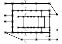
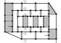
Figure 8: Progress of Algorithm 4 on a good $3$-outerplanar embedding (same as in Figure 6). The shaded areas demarcate the subnetworks already assembled. Left assembly: after initialization, Middle assembly: after first iteration, Right assembly: after second iteration.

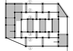
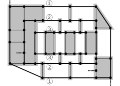
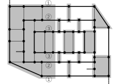
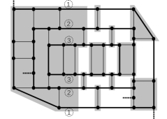
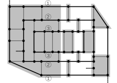
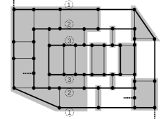
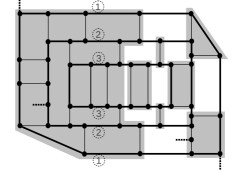
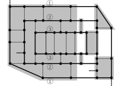
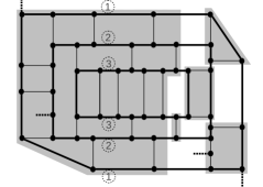
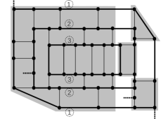
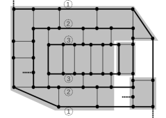
Figure 9: Progress of Algorithm 4 on a good $3$-outerplanar embedding (same as in Figure 6) during the main iteration.

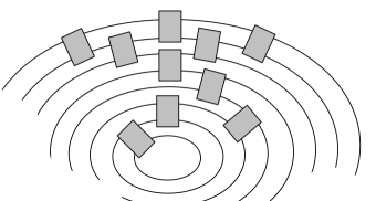
Figure 10: Two possible configurations of assembled subnetworks, in a good $8$-outerplanar embedding, at the end of the second iteration of Algorithm 4.

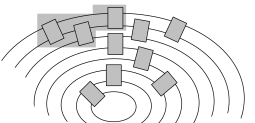
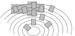
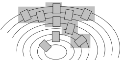
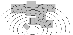
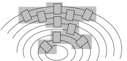
Figure 11: Progress of Algorithm 4 during its main iteration, starting from the configuration on the right in Figure 10.

Appendix D Appendix: Further Comments for Section 6

Beyond the future work mentioned in Section 6, we here mention two other areas of future research. These will build on results already obtained and provide a wider range of useful applications in system modeling and analysis. The second area below (Subsection D.2) was alluded to earlier, in footnote 12 and in Example 11. They should separately open a different line of investigation.

D.1 Algebraic Characterization of Principality

A typing $T$ is a function of the form $T:\mathscr{P}(\mathbf{A}_{\text{in,out}})\to{\cal I}(\mathbb{R})$, but not every function of this form is a typing of some network. To be a network typing, such a function must satisfy certain conditions. For example, it must always be such that $T(\varnothing)=T(\mathbf{A}_{\text{in,out}})=[0,0]=\{0\}$. Another necessary condition is expressed by the conclusion of Lemma 12 (there are simple examples, with $|\,\mathbf{A}_{\text{in,out}}\,|\geqslant 4$, showing this condition is not sufficient to make $T$ a principal typing). Tasks ahead include the following:

1. Define an algebraic characterization, preferably in the form of necessary and sufficient conditions, such that a partial function $T:\mathscr{P}(\mathbf{A}_{\text{in,out}})\to{\cal I}(\mathbb{R})$ satisfies these conditions iff there exists a network ${\cal N}$ of which $T$ is the principal typing.

2. Once such an algebraic characterization is established, develop an implementation methodology which, given a $T:\mathscr{P}(\mathbf{A}_{\text{in,out}})\to{\cal I}(\mathbb{R})$ satisfying it, can be used to implement $T$ in the form of a network ${\cal N}$. More precisely, given such a $T$, develop a methodology to construct a network ${\cal N}$ such that $T$ is the principal typing of ${\cal N}$.

3. Refine this implementation methodology so that it constructs a smallest-size network ${\cal N}$ for which $T$ is the principal typing. Such a network ${\cal N}$ can be viewed as the “best” implementation of the given $T$.

When the external dimension $|\,\mathbf{A}_{\text{in,out}}\,|=2$, with one input arc $a_{1}$ and one output arc $a_{2}$, these questions are trivial. In such a case, $T$ is the principal typing of some network iff there are numbers $0\leqslant r\leqslant s$ such that

$$T(\varnothing)=T(\{a_{1},a_{2}\})=[0,0],\quad T(\{a_{1}\})=[r,s],\quad T(\{a_{2}\})=[-s,-r].$$

For such a $T$, there is always a one-node implementation.

When the external dimension $|\,\mathbf{A}_{\text{in,out}}\,|=3$, with, say, input arcs $\{a_{1},a_{2}\}$ and output arc $a_{3}$, these questions are again easy. In such a case, $T$ is the principal typing of some network iff there are numbers $0\leqslant r_{i}\leqslant s_{i}$, for every $i\in\{1,2,3\}$, such that:

$$T(\varnothing)\ =\ \ \ T(\{a_{1},a_{2},a_{3}\})\ =\ [0,0],$$

$$T(\{a_{1}\})\ =\ -T(\{a_{2},a_{3}\})\ =\ [r_{1},s_{2}],$$

$$T(\{a_{2}\})\ =\ -T(\{a_{1},a_{3}\})\ =\ [r_{2},s_{2}],$$

$$T(\{a_{3}\})\ =\ -T(\{a_{1},a_{2}\})\ =\ [-s_{3},-r_{3}],$$

where $r_{1}+r_{2}=r_{3}$ and $\max\{s_{1},s_{2}\}\leqslant s_{3}\leqslant s_{1}+s_{2}$. For such a $T$, there is always a one-node implementation.

The problem becomes interesting and non-trivial when $|\,\mathbf{A}_{\text{in,out}}\,|\geqslant 4$. For a sense of the difficulty in such a case, consider the network ${\cal N}_{2}$ in Example 10. It is not the smallest-size implementation of the typing $T_{2}$ in Example 10, as illustrated by the next example.

Example 36.

The network ${\cal N}_{4}$ in Figure 12 was obtained by brute-force trial-and-error. It is equivalent to ${\cal N}_{2}$ in Example 10, and qualifies as a better implementation of $T_{2}$, because ${\cal N}_{4}$ has fewer nodes than ${\cal N}_{2}$, with $6$ nodes in ${\cal N}_{4}$ against $8$ nodes in ${\cal N}_{2}$. (We can also compare network sizes by counting both nodes and arcs: $6+12=18$ in ${\cal N}_{4}$ against $8+16=24$ in ${\cal N}_{2}$.) $\square$

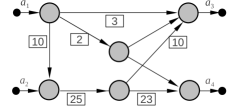
Figure 12: For Example 36: Network ${\cal N}_{4}$ is equivalent to ${\cal N}_{2}$ in Example 10, but is a better implementation of the same principal typing $T_{2}$. Missing lower bounds are $0$, missing upper bounds are a “very large number” $K$.

We conjecture that, if $|\,\mathbf{A}_{\text{in,out}}\,|=4$ and $T:\mathscr{P}(\mathbf{A}_{\text{in,out}})\to{\cal I}(\mathbb{R})$ is the principal typing of some network with external arcs $\mathbf{A}_{\text{in,out}}$, then there is a smallest-size implementation of $T$ requiring at most $6$ nodes.

D.2 Angelic Non-Determinism versus Demonic Non-Determinism

Suppose $\mathscr{A}$ is a large assembly of networks containing network ${\cal M}$ as a subnetwork. Under what conditions can we safely substitute another network ${\cal N}$ for ${\cal M}$? A minimal requirement is that ${\cal M}$ and ${\cal N}$ are similar, i.e., they have the same number of input arcs and the same number of output arcs. If we are given principal typings $T$ and $U$ for ${\cal M}$ and ${\cal N}$, respectively, we should have enough information to decide whether the substitution is safe. To simplify a little, let the input and output arcs of ${\cal M}$ and ${\cal N}$ be $\mathbf{A}_{\text{in}}=\{a_{1},a_{2}\}$ and $\mathbf{A}_{\text{out}}=\{a_{3},a_{4}\}$. If the substitution of ${\cal N}$ for ${\cal M}$ is safe, then ${\cal N}$ should be able to consume every input flow that ${\cal M}$ is able to consume, i.e., if an input assignment $f_{\text{in}}:\{a_{1},a_{2}\}\to\mathbb{R}_{+}$ satisfies $[T]_{\mathscr{P}(\{a_{1},a_{2}\})}$, then it must also satisfy $[U]_{\mathscr{P}(\{a_{1},a_{2}\})}$. Hence, the following inclusions are a reasonable requirement for safe substitution:

• $T(\{a_{1}\})\subseteq U(\{a_{1}\}),\quad T(\{a_{2}\})\subseteq U(\{a_{2}\}),\quad\text{and}\quad T(\{a_{1},a_{2}\})\subseteq U(\{a_{1},a_{2}\}).$

Symmetrically, for safe substitution, every output flow produced by ${\cal N}$ should not exceed the limits of an output flow produced by ${\cal M}$, i.e., if an input assignment $f_{\text{out}}:\{a_{3},a_{4}\}\to\mathbb{R}_{+}$ satisfies $[U]_{\mathscr{P}(\{a_{3},a_{4}\})}$, then it must also satisfy $[T]_{\mathscr{P}(\{a_{3},a_{4}\})}$. Hence, another reasonable requirement consists of the following reversed inclusions:

• $T(\{a_{3}\})\supseteq U(\{a_{3}\}),\quad T(\{a_{4}\})\supseteq U(\{a_{4}\}),\quad\text{and}\quad T(\{a_{3},a_{4}\})\supseteq U(\{a_{3},a_{4}\}).$

If $U$ satisfies both $({\dagger})$ and $({\ddagger})$, is the substitution of ${\cal N}$ for ${\cal M}$ in $\mathscr{A}$ safe? It depends. Conditions $({\dagger})$ and $({\ddagger})$ are necessary, but there are other issues which we elaborate in the next example.

Example 37.

In the larger assembly $\mathscr{A}$ described above, let ${\cal M}={\cal N}_{3}$ from Example 11 and ${\cal N}={\cal N}_{2}$ from Example 10. We have the following relationship $T_{2}<:T_{3}$, where “$<:$” is the subtyping relation, defined in Examples 10 and 11. More, in fact, $T=T_{3}$ and $U=T_{2}$ satisfy both conditions $({\dagger})$ and $({\ddagger})$, which are therefore not sufficient to prevent the unsafe situation we now describe.

As we explain below, if ${\cal N}_{2}$ operates in a way to preserve the feasibility of flows in $\mathscr{A}$, i.e., if it operates angelically and tries to keep $\mathscr{A}$ in good working order, then replacing ${\cal N}_{3}$ by ${\cal N}_{2}$ is safe. However, if ${\cal N}_{2}$ makes choices that disrupt $\mathscr{A}$’s good working order, maliciously or unintentionally, i.e., if it operates demonically and violates the feasibility of flows in $\mathscr{A}$, then the substitution is unsafe. This can happen because for the same assignment $f_{\text{in}}$ to the input arcs (resp., the same assignment $f_{\text{out}}$ to the output arcs), corresponds several possible output assignments $f_{\text{out}}$ (resp., input assignments $f_{\text{in}}$), without violating any of ${\cal N}_{2}$’s internal constraints.

Suppose ${\cal N}_{3}$ in $\mathscr{A}$ is prompted to consume some flow entering at input arcs $a_{1}$ and $a_{2}$. (A similar and symmetric argument can be made when ${\cal N}_{3}$ is asked to produce some flow at output arcs $a_{3}$ and $a_{4}$.) Suppose the incoming flow is given by the assignment $f_{\text{in}}(a_{1})=15$ and $f_{\text{in}}(a_{2})=0$. Flow is then pushed along the internal arcs of ${\cal N}_{3}$, respecting capacity constraints and flow conservation at nodes. There are many different ways in which flow can be pushed through. By direct inspection, relative to the given $f_{\text{in}}$, the largest possible quantity exiting at output arc $a_{4}$ is $10$. So, relative to the given $f_{\text{in}}$, the output assignment which is most skewed in favor of $a_{4}$ is $f_{\text{out}}(a_{3})=5$ and $f_{\text{out}}(a_{4})=10$.

Under the assumption that $\mathscr{A}$ works safely with ${\cal N}_{3}$ inserted, we take this conclusion to mean that any output quantity exceeding $10$ at arc $a_{4}$, when $f_{\text{in}}(a_{1})=15$ and $f_{\text{in}}(a_{2})=0$, disrupts $\mathscr{A}$’s overall operation. For a concrete situation, when $f_{\text{in}}(a_{1})=15$ and $f_{\text{in}}(a_{2})=0$, it can occur that the $10$ units exiting from $a_{4}$ enter some node $\nu$ in $\mathscr{A}$ and cannot be increased without violating a capacity constraint on an arc exiting $\nu$.

Next, suppose we substitute ${\cal N}_{2}$ for ${\cal N}_{3}$ and examine ${\cal N}_{2}$’s behavior with the same $f_{\text{in}}(a_{1})=15$ and $f_{\text{in}}(a_{2})=0$. By inspection, the flow that is most skewed in favor of $a_{4}$ gives rise to the output assignment $f_{\text{out}}(a_{3})=3$ and $f_{\text{out}}(a_{4})=12$. In this case, the output quantity at $a_{4}$ exceeds $10$, which, as argued above, is disruptive of $\mathscr{A}$’s overall operation. Note that the presumed disruption occurs in the enclosing context that is part of $\mathscr{A}$, not inside ${\cal N}_{2}$ itself, where flow is still directed by respecting flow conservation at ${\cal N}_{2}$’s nodes and lower-bound/upper-bound capacities at ${\cal N}_{2}$’s arcs. Thus, ${\cal N}_{2}$’s harmful behavior is not the result of violating its own internal constraints, but of its malicious or (unintended) faulty interaction with the enclosing context.

Consider now a slight adjustment of ${\cal N}_{3}$, call it ${\cal N}_{3}^{\prime}$, where we make a single change in ${\cal N}_{3}$, namely, in the upper-bound capacity of input arc $a_{1}$: Decrease $\overline{\bm{c}}(a_{1})$ from $K$ (“very large number”) to $10$. The typing $T_{3}$ is no longer principal for ${\cal N}_{3}^{\prime}$. We compute a new principal typing $T_{3}^{\prime}$ for ${\cal N}_{3}^{\prime}$ which, in addition to the type assignments $T_{3}^{\prime}(\varnothing)=T_{3}^{\prime}(\{a_{1},a_{2},a_{3},a_{4}\})=[0,0]$, makes the following type assignments:

$$\underline{a_{1}:[0,10]}\quad a_{2}:[0,25]\quad -a_{3}:[-15,0]\quad -a_{4}:[-25,0]$$

$$a_{1}+a_{2}:[0,30]\quad a_{1}-a_{3}:[-10,10]\quad \underline{a_{1}-a_{4}:[-23,10]}$$

$$\underline{a_{2}-a_{3}:[-10,23]}\quad a_{2}-a_{4}:[-10,10] -a_{3}-a_{4}:[-30,0]\quad$$

$$a_{1}+a_{2}-a_{3}:[0,25]\qquad a_{1}+a_{2}-a_{4}:[0,15]\qquad a_{1}-a_{3}-a_{4}:[-23,0]\qquad \underline{a_{2}-a_{3}-a_{4}:[-10,0]}\quad$$

The underlined type assignments here are those that differ from the corresponding type assignments made by $T_{3}$. It is easy to check that, however demonically ${\cal N}_{2}$ chooses to push flow through its internal arcs, the substitution of ${\cal N}_{2}$ for ${\cal N}_{3}^{\prime}$ is “input safe”; i.e., for every input assignment $f_{\text{in}}:\{a_{1},a_{2}\}\to\mathbb{R}_{+}$ satisfying $[T_{3}^{\prime}]_{\mathscr{P}(\{a_{1},a_{2}\})}$, and every extension $g:\{a_{1},a_{2},a_{3},a_{4}\}\to\mathbb{R}_{+}$ of $f_{\text{in}}$, the IO assignment $g$ satisfies $T_{2}$ iff $g$ satisfies $T_{3}^{\prime}$.

Similarly, consider an outgoing flow in ${\cal N}_{3}$ given by the assignment $f_{\text{out}}(a_{3})=0$ and $f_{\text{out}}(a_{4})=25$. Relative to this $f_{\text{out}}$, consider the entering flow at $\{a_{1},a_{2}\}$ which is most skewed in favor of $a_{1}$. By inspection, this is the input assignment $f_{\text{in}}(a_{1})=10$ and $f_{\text{in}}(a_{2})=15$. By contrast in ${\cal N}_{2}$, if $f_{\text{out}}(a_{3})=0$ and $f_{\text{out}}(a_{4})=25$, then the corresponding input assignment which is most skewed in favor of $a_{1}$ is $f_{\text{in}}(a_{1})=12$ and $f_{\text{in}}(a_{2})=13$.

We can adjust ${\cal N}_{3}$, to define another network ${\cal N}_{3}^{\prime\prime}$, for which the substitution of ${\cal N}_{2}$ is “output safe”. ${\cal N}_{3}^{\prime\prime}$ is obtained by making a single change: Decrease $\overline{\bm{c}}(a_{4})$ from $K$ (“very large number”) to $10$. The principal typing $T_{3}^{\prime\prime}$ for ${\cal N}_{3}^{\prime\prime}$ makes the type assignments $T_{3}^{\prime\prime}(\varnothing)=T_{3}^{\prime\prime}(\{a_{1},a_{2},a_{3},a_{4}\})=[0,0]$ in addition to:

$$a_{1}:[0,15]\quad \underline{a_{2}:[0,20]}\quad -a_{3}:[-15,0]\quad \underline{-a_{4}:[-10,0]}$$

$$\underline{a_{1}+a_{2}:[0,25]}\quad a_{1}-a_{3}:[-10,10]\quad \underline{a_{1}-a_{4}:[-10,15]}$$

$$\underline{a_{2}-a_{3}:[-15,10]}\quad a_{2}-a_{4}:[-10,10] -a_{3}-a_{4}:[-25,0]\quad$$

$$\underline{a_{1}+a_{2}-a_{3}:[0,10]}\qquad a_{1}+a_{2}-a_{4}:[0,15]\qquad \underline{a_{1}-a_{3}-a_{4}:[-20,0]}\qquad a_{2}-a_{3}-a_{4}:[-15,0]\quad$$

Finally, we can make both of the preceding adjustments in ${\cal N}_{3}$: Decrease both $\overline{\bm{c}}(a_{1})$ and $\overline{\bm{c}}(a_{4})$ from $K$ (“very large number”) to $10$, so that the substitution of ${\cal N}_{2}$ is both “input safe” and “output safe”. $\square$

Based on the discussion in Example 37, in the presence of demonic non-determinism, we need a notion of subtyping more restrictive than “$<:$”, which we call “strong subtyping” and denote by “$\ll:$”.

Definition 38 (Strong Subtyping).

Let $T,U:\mathscr{P}(\mathbf{A}_{\text{in,out}})\to{\cal I}(\mathbb{R})$ be principal typings for similar networks ${\cal M}$ and ${\cal N}$, respectively, both with the same set $\mathbf{A}_{\text{in,out}}$ of input/output arcs. We say $T$ is input-safe for $U$ iff:

• For every $f_{\text{in}}:\mathbf{A}_{\text{in}}\to\mathbb{R}_{+}$ satisfying $[T]_{\mathscr{P}(\mathbf{A}_{\text{in}})}$, and for every $g:\mathbf{A}_{\text{in,out}}\to\mathbb{R}_{+}$ extending $f_{\text{in}}$, it holds that:
  $g$ satisfies $T$ $\Leftrightarrow$ $g$ satisfies $U$.

We say $T$ is output-safe for $U$ iff:

• For every $f_{\text{out}}:\mathbf{A}_{\text{out}}\to\mathbb{R}_{+}$ satisfying $[T]_{\mathscr{P}(\mathbf{A}_{\text{out}})}$, and for every $g:\mathbf{A}_{\text{in,out}}\to\mathbb{R}_{+}$ extending $f_{\text{out}}$, it holds that: $g$ satisfies $T$ $\Leftrightarrow$ $g$ satisfies $U$.

We say $T$ is safe for $U$, or say $U$ is a strong subtyping of $T$ and write $U\ll:T$, iff $T$ is both input-safe and output-safe for $U$. Strong subtyping expresses the condition for the safe substitution of ${\cal N}$ (whose principal typing is $U$) for ${\cal M}$ (whose principal typing is $T$) in the presence of demonic non-determinism. $\square$

We state without proof some simple properties of “$\ll:$”, the starting point of an investigation of how to extend our typing theory to handle demonic non-determinism.

Fact 39 (Strong Subtyping is a Partial Order).

Let $S,T,U:\mathscr{P}(\mathbf{A}_{\text{\rm in,out}})\to{\cal I}(\mathbb{R})$ be principal typings (of some similar networks) over the same input/output set $\mathbf{A}_{\text{\rm in,out}}$.

1. $T\ll:T$ (reflexivity).

2. If $T\ll:U$ and $U\ll:T$, then $T=U$ (anti-symmetry).

3. If $S\ll:T$ and $T\ll:U$, then $S\ll:U$ (transitivity).

4. If $T\ll:U$, then $T<:U$, but not the other way around in general. (A counter-example for the converse is in Example 37, where $T_{2}<:T_{3}$ but $T_{2}\not{\ll}:T_{3}$.)

Points 1-3 say that “$\ll:$” is a partial order, just as “$<:$” is, and point 4 says that this partial order can be embedded in the partial order of “$<:$”.

References

- [1] R.K. Ahuja, T. L. Magnanti, and J.B. Orlin. Network Flows: Theory, Algorithms, and Applications. Prentice Hall, Englewood Cliffs, N.J., 1993.
- [2] Takao Asano and Yasuhito Asano. Recent Developments in Maximum Flow Algorithms. Journal of the Operations Research Society of Japan, 43(1), March 2000.
- [3] S. Balon and G. Leduc. Dividing the Traffic Matrix to Approach Optimal Traffic Engineering. In 14th IEEE Int’l Conf. on Networks (ICON 2006), volume 2, pages 566–571, September 2006.
- [4] A. Bestavros, A. Kfoury, A. Lapets, and M. Ocean. Safe Compositional Network Sketches: Tool and Use Cases. In IEEE Workshop on Compositional Theory and Technology for Real-Time Embedded Systems, Wash D.C., December 2009.
- [5] A. Bestavros, A. Kfoury, A. Lapets, and M. Ocean. Safe Compositional Network Sketches: The Formal Framework. In 13th ACM HSCC, Stockholm, April 2010.
- [6] Azer Bestavros and Assaf Kfoury. A Domain-Specific Language for Incremental and Modular Design of Large-Scale Verifiably-Safe Flow Networks. In Proc. of IFIP Working Conference on Domain-Specific Languages (DSL 2011), EPTCS Volume 66, pages 24–47, Sept 2011.
- [7] Hans L. Bodlaender. A Partial -Arboretum of Graphs with Bounded Treewidth. Theoretical Computer Science, 209(1-2):1–45, 1998.
- [8] Glencora Borradaile and Philip Klein. An Algorithm for Maximum st-Flow in a Directed Planar Graph. Journal of the ACM, 56(2):1–30, April 2009.
- [9] Glencora Borradaile, Philip Klein, Shay Mozes, Yahav Nussbaum, and Christian Wulff-Nilsen. Multiple-Source Multiple-Sink Maximum Flow in Directed Planar Graphs in Near-Linear Time. In FOCS 2011, Proc. of 52nd Annual Symposium on Foundations of Computer Science, pages 170–179. IEEE, October 2011.
- [10] S. Boyd and L. Vanderberghe. Convex Optimization. Cambridge University Press, New York, USA, (second printing with corrections) 2009.
- [11] Stephen P. Bradley, Arnoldo C. Hax, and Thomas L. Magnanti. Applied Mathematical Programming. Addison-Wesley, Reading, MA, 1977.
- [12] Bala G. Chandran and Dorit S. Hochbaum. A Computational Study of the Pseudoflow and Push-Relabel Algorithms for the Maximum Flow Problem. Oper. Res., 57(2):358–376, March/April 2009.
- [13] Swarat Chaudhuri, Sumit Gulwani, and Roberto Lublinerman. Continuity and Robustness of Programs. Commun. ACM, 55(8):107–115, August 2012.
- [14] Swarat Chaudhuri, Sumit Gulwani, Roberto Lublinerman, and Sara Navidpour. Proving Programs Robust. In Proc. of 19th ACM SIGSOFT Symposium and the 13th European Conference on Foundations of Software Engineering, ESEC/FSE ’11, pages 102–112, New York, NY, USA, 2011. ACM.
- [15] Paul Christiano, Jonathan A. Kelner, Aleksander Madry, Daniel A. Spielman, and Shang-Hua Teng. Electrical Flows, Laplacian Systems, and Faster Approximation of Maximum Flow in Undirected Graphs. In L. Fortnow and S. P. Vadhan, editors, STOC 2011, Proc. of 43rd Symp. on Theory of Computing, pages 273–282. ACM, 2011.
- [16] Loris D’Antoni, Marco Gaboardi, Emilio Jesús Gallego Arias, Andreas Haeberlen, and Benjamin Pierce. Sensitivity Analysis Using Type-Based Constraints. In Proc. of 1st Annual Workshop on Functional Programming Concepts in Domain-Specific Languages, FPCDSL ’13, pages 43–50, New York, NY, USA, 2013. ACM.
- [17] Samir Datta and Prakriya. Planarity Testing Revisited. Electronic Colloquium on Computational Complexity, 9, 2011.
- [18] Reinhard Deistel. Graph Theory. Springer Verlag, 2012.
- [19] E.A. Dinic. Algorithm for Solution of a Problem of Maximum Flow in Networks with Power Estimation. Soviet Mathematics Doklady, 11:1277–1280, 1970.
- [20] David Eisenstat and Philip N. Klein. Linear-Time Algorithms for Max Flow and Multiple-Source Shortest Paths in Unit-Weight Planar Graphs. In STOC 2013, Proc. of 45th Symp. on Theory of Computing, pages 735–744, June 2013.
- [21] L.R. Ford and D.R. Fulkerson. Maximal Flow Through a Network. Canadian Journal of Mathematics, 8:399–404, 1956.
- [22] Alexandru Florian Gaiu. Sequential Parameter Tuning of Algorithms for the Vehicle Routing Problem. Technical Report Internal Report 2013-04, Computer Science Department, Universiteit Leiden, February 2013.
- [23] Andrew V. Goldberg. A New Max-Flow Algorithm. Technical Report MIT/LCS/TM-291, Laboratory for Computer Science, MIT, 1985.
- [24] Andrew V. Goldberg. Recent Developments in Maximum Flow Algorithms (Invited Lecture). In SWAT ’98: Proc. of 6th Scandinavian Workshop on Algorithm Theory, pages 1–10. Springer Verlag, 1998.
- [25] Andrew V. Goldberg. Two-Level Push-Relabel Algorithm for the Maximum Flow Problem. In Proc. of 5th International Conference on Algorithmic Aspects in Information and Management, AAIM ’09, pages 212–225, Berlin, Heidelberg, 2009. Springer-Verlag.
- [26] Andrew V. Goldberg and Satish Rao. Beyond the Flow Decomposition Barrier. J. ACM, 45(5):783–797, September 1998.
- [27] Andrew V. Goldberg and Robert E. Tarjan. A New Approach to the Maximum Flow Problem. In STOC 1986, Proc. of 18th Annual ACM Symposium on the Theory of Computing, pages 136–146, 1986.
- [28] Torben Hagerup, Jyrki Katajainen, Naomi Nishimura, and Prabhakar Ragde. Characterizing Multiterminal Flow Networks and Computing Flows in Networks of Small Treewidth. Journal of Computer and System Sciences, 57(3):366–375, December 1998.
- [29] Dorit S. Hochbaum. The Pseudoflow Algorithm: A New Algorithm for the Maximum-Flow Problem. Oper. Res., 56(4):992–1009, July 2008.
- [30] Trevor Jim. What Are Principal Typings and What Are They Good For? Tech. memo. MIT/LCS/TM-532, MIT, 1995.
- [31] Trevor Jim. What Are Principal Typings and What Are They Good For? In Proc. of 23rd ACM Symp. on Principles of Programming Languages, pages 42–53, 1996.
- [32] Frank Kammer. Determining the Smallest Such That Is -Outerplanar. In Lars Arge, Michael Hoffmann, and Emo Welzl, editors, Proc. of 15th Annual European Symposium on Algorithms, ESA 2007, pages 359–370. LNCS 4698, Springer Verlag, September 2007.
- [33] Jonathan A. Kelner, Lorenzo Orecchia, Yin Tat Lee, and Aaron Sidford. An Almost-Linear-Time Algorithm for Approximate Max Flow in Undirected Graphs, and its Multicommodity Generalizations. Computing Research Repository (CoRR), abs/1304.2338, 2013.
- [34] Assaf Kfoury. A Domain-Specific Language for Incremental and Modular Design of Large-Scale Verifiably-Safe Flow Networks (Part 1). Technical Report BUCS-TR-2011-011, CS Dept, Boston Univ, May 2011.
- [35] Assaf Kfoury. The Denotational, Operational, and Static Semantics of a Domain-Specific Language for the Design of Flow Networks. In Proc. of SBLP 2011: Brazilian Symposium on Programming Languages, Sept 2011.
- [36] Assaf Kfoury. A Typing Theory for Flow Networks (Part I), CS Dept, Boston Univ, BUCS-TR-2012-021. http://www.cs.bu.edu/techreports/pdf/2012-021-cfn-typing-theory-a.pdf, December 2012.
- [37] Assaf Kfoury. A Compositional Approach to Network Algorithms. Technical Report BUCS-TR-2013-015, CS Dept, Boston University, November 2013.
- [38] Philip N. Klein. Optimization Algorithms for Planar Graphs. http://planarity.org/, 2012.
- [39] Jakub Lacki, Yahav Nussbaum, Piotr Sankowski, and Christian Wulff-Nilsen. Single Source – All Sinks Max Flows in Planar Digraphs. In IEEE 53rd Annual Symposium on Foundations of Computer Science, volume 0 of FOCS ’11, pages 599–608, Los Alamitos, CA, USA, 2012. IEEE Computer Society.
- [40] Yin Tat Lee, Satish Rao, and Nikhil Srivastava. A New Approach to Computing Maximum Flows Using Electrical Flows. In STOC 2013, Proc. of 45th Symp. on Theory of Computing, pages 755–764. ACM, June 2013.
- [41] G. Mazzoni, S. Pallottino, and M.G. Scutella. The Maximum Flow Problem: A Max-Preflow Approach. European Journal of Operational Research, 53:257–278, 1991.
- [42] Takao Nishizeki and Md. Saidur Rahman. Rectangular Drawing Algorithms. In Roberto Tamassia, editor, Hanbook of Graph Drawing and Visualization, pages 317–348. CRC Press, Baton Rouge, FL, 2013.
- [43] James B. Orlin. Max Flows in Time or Less. In STOC 2013, Proc. of 45th Symposium on the Theory of Computing, pages 765–774. ACM, June 2013.
- [44] Maurizio Patrignani. Planarity Testing and Embedding. In Roberto Tamassia, editor, Hanbook of Graph Drawing and Visualization, pages 1–42. CRC Press, Baton Rouge, FL, 2013.
- [45] A. Schrijver. A Course in Combinatorial Optimization. CWI (the manuscript can be downloaded from the author’s webpage http://homepages.cwi.nl/~lex/), Amsterdam, The Netherlands, 2012.
- [46] Jonah Sherman. Nearly Maximum Flows in Nearly Linear Time. Computing Research Repository (CoRR), abs/1304.2077 (also in Proc. of FOCS 2013), 2013.
- [47] Nate Soule, Azer Bestavros, Assaf Kfoury, and Andrei Lapets. Safe Compositional Equation-based Modeling of Constrained Flow Networks. In Proc. of 4th Int’l Workshop on Equation-Based Object-Oriented Modeling Languages and Tools, Zürich, September 2011.