Three-Dimensional Multicomponent Vesicles: Dynamics & Influence of Material Properties

Abstract

In this work, the nonlinear dynamics of a fully three-dimensional multicomponent vesicle in shear flow are explored. Using a volume- and area-conserving projection method coupled to a gradient-augmented level set and surface phase method, the dynamics are systematically studied as a function of the membrane bending rigidity difference between the components, the speed of diffusion compared to the underlying shear flow, and the strength of the phase domain energy compared to the bending energy. Using a pre-segregated vesicle, three dynamics are observed: stationary phase, phase-treading, and a new dynamic called vertical banding. These regimes are very sensitive to the strength of the domain line energy, as the vertical banding regime is not observed when line energy is larger than the bending energy. These findings demonstrate that a complete understanding of multicomponent vesicle dynamics require that the full three-dimensional system be modeled, and show the complexity obtained when considering heterogeneous material properties.

I Introduction

Biological cells have a bilayer membrane which protects the enclosed material and acts as a medium of communication between the intra- and extra-cellular environments. Variation in the composition of the membrane have shown to impact fundamental cellular processes such as signal transduction Simons and Toomre (2000); Sackmann and Smith (2014), membrane trafficking Simons and Vaz (2004), and membrane sorting Mukherjee and Maxfield (2004). The inhomogeneous membranes of living cells have a complex and a dynamic structure and thus the simplified membrane model system of lipid vesicles is of major significance Lipowsky and Sackmann (1995).

A multicomponent membrane of a vesicle is typically composed of a mixture of saturated lipids, unsaturated lipids, and cholesterol. Due to the molecular structure, saturated lipids tend to combine with cholesterol to form energetically stable and relatively ordered domains, also known as an ordered phase Baumgart et al. (2003); Veatch and Keller (2003). These are surrounded by the unsaturated lipids, known as the disordered phase, and the process of phase segregation occurs to achieve a lower state of energy Veatch and Keller (2005). In general, the phases have differing material properties, which causes morphological changes to the underlying surface of the vesicle, as observed in experiments Baumgart et al. (2005, 2003); McMahon and Gallop (2005). While not considered here, variation of the domains between the inner and outer leaflet have also been shown to influence the overall material properties and dynamics Lu et al. (2016).

Extensive work in the literature is present for a single component membrane Deschamps et al. (2009); Biben and Misbah (2003); Aranda et al. (2008); Staykova et al. (2008); Vlahovska et al. (2009); Kolahdouz and Salac (2015); Salac and Miksis (2012); Vlahovska and Gracia (2007); Kantsler et al. (2008), but there is limited work for inhomogeneous vesicles Elliott and Stinner (2013, 2010); Barrett et al. (2017). In cases where multicomponent vesicles are studied, material properties, such as the bending rigidity, have been shown to dramatically influence the dynamics Allain and Ben Amar (2004); Fournier and Ben Amar (2006). Du et al. demonstrated interesting and exotic dynamic patterns in 3D multicomponent vesicles Wang and Du (2008). Funkhouser et al. examined the dynamics of vesicles with non-uniform mechanical properties Funkhouser et al. (2014). These works are however done in absence of an aqueous medium. Other works which include the influence of the fluid are limited to two-dimensions, which cannot include all aspects of multicomponent vesicle such as the line energy associated with domain boundaries Liu et al. (2017).

In this work, the hydrodynamics of a three-dimensional multicomponent vesicle in shear flow is systematically explored. The goal of this work is to investigate and understand the influence of material properties on the dynamics of multicomponent vesicles in the presence of shear flow. To the best of the authors’ knowledge, this is the first work to carry out such an investigation in three-dimensional space. The parameters considered are the membrane bending rigidity, the rate of surface diffusion, and the influence of the domain line energy. Using the model presented here, three major dynamics are observed: stationary phases, vertical stationary band, and the treading of the surface phases. Using two characteristic values of domain line energy, the phase diagrams of these dynamics as a function of surface diffusion rate and membrane bending rigidity is presented. An extensive investigation is performed and sample dynamics, energy curves, treading period, and time for domain merging are presented.

The remainder of this work describes the models and numerical methods used. This is followed by a demonstration of the major observed dynamics. Considering two characteristic domain line energy values, a systematic investigation of the dynamics as a function of the surface diffusion rate and bending rigidity difference is performed. This is followed by further discussion and conclusions.

II Model and Methods

Consider a multicomponent vesicle suspended in an aqueous fluid that differs from the fluid encapsulated inside the membrane. The membrane $\Gamma$ separates the fluid outside $\Omega^{+}$ from the fluid inside $\Omega^{-}$ as shown in Fig. 1. The vesicle is characterized using a reduced volume parameter $\nu$, which is defined as the ratio of the vesicle volume $V$ to the volume of a sphere with the same surface area $A$: $\nu=3V/4\pi a^{3}$, where $a=\sqrt{A/4\pi}$. The vesicles considered here have a radius $\sim 10\mu$m and a membrane thickness of $\sim 5$ nm, and therefore the membrane is considered as an infinitesimally thin interface. Additionally, the membrane is impermeable to fluids and the number of lipid molecules on the surface of the membrane does not change over time, which results in an inextensible membrane. Therefore, such systems are both volume and surface area conserving.

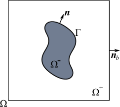
Figure 1: A vesicle membrane $\Gamma$ separating the fluid outside $\Omega^{+}$ from the fluid inside $\Omega^{-}$.

II.1 Fluid Field

In general, such systems are governed by the Navier-Stokes equation and a volume-incompressibility constraint,

$$\rho\dfrac{D\boldsymbol{u}^{\pm}}{Dt}=\nabla\cdot\boldsymbol{T}_{hd}^{\pm}\text{\hskip 8.53581pt and \hskip 8.53581pt}\nabla\cdot\boldsymbol{u}^{\pm}=0\hskip 8.53581pt\text{in \hskip 8.53581pt}\Omega^{\pm},$$

where $\rho$ is the density, $\boldsymbol{u}$ is the fluid velocity vector, and $\boldsymbol{T}_{hd}$ is the bulk hydrodynamic stress tensor. This tensor is given by

$$\boldsymbol{T}_{hd}=-p^{\pm}\boldsymbol{I}+\mu^{\pm}(\nabla\boldsymbol{u}^{\pm}+\nabla^{T}\boldsymbol{u}^{\pm})\hskip 8.53581pt\text{in \hskip 8.53581pt}\Omega^{\pm},$$ (1)

where $p$ is the pressure and $\mu$ is the fluid viscosity.

The inextensible membrane introduces three additional conditions. First, the velocity on the surface of the membrane is assumed to be continuous $[\boldsymbol{u}]=0$, where $[\cdot]$ represents the jump of a parameter across the interface. Second, the hydrodynamic stress tensor undergoes a jump across the interface which is balanced by the forces exerted by the membrane,

$$\boldsymbol{n}\cdot[\boldsymbol{T}_{hd}]=\boldsymbol{f},$$ (2)

where $\boldsymbol{f}$ is the total membrane force. Finally, since the membrane area is conserved, the local area is conserved via a surface-incompressibility constraint on the fluid field,

$$\nabla_{s}\cdot\boldsymbol{u}=0\hskip 8.53581pt\text{on}\hskip 8.53581pt\Gamma.$$

II.2 Surface Material Field

The membrane surface of the vesicle is composed of saturated lipids that combine with cholesterol to form energetically stable domains also known as the ordered phase. The ordered phase is surrounded by unsaturated lipids, also called the disordered phase. To model the multicomponent surface dynamics, a two phase Cahn-Hilliard system is used. Consider one surface phase $B$ with surface concentration $q(\boldsymbol{x},t)$ while $1-q(\boldsymbol{x},t)$ indicates the amount of the second, $A$ phase. There is no mass transfer from the bulk to the interface or vice versa, and therefore the mass of the surface concentration is conserved,

$$M_{q}(t)=\int_{\Gamma(t)}q(\boldsymbol{x},t)=M_{q}(0).$$ (3)

This surface concentration evolves on the interface via a mass-conserving convection-diffusion equation, which in Eulerian form is written as

$$\dfrac{\partial q}{\partial t}+\boldsymbol{u}\cdot\nabla q=\nabla_{s}\cdot\boldsymbol{J}_{s},$$ (4)

where $J_{s}$ is the surface flux and is defined in the next section. Note that the advection as written accounts for motion both in the tangential direction and in the normal direction, which accounts for movement of the interface.

II.3 Constitutive Equations

The total energy of the system, $E$, consists of three contributions:

$$E=E_{b}+E_{\gamma}+E_{q},$$ (5)

where

$$E_{b} =\int_{\Gamma}\dfrac{\kappa_{c}(q)}{2}H^{2}\;\textrm{dA},$$ (6)

$$E_{\gamma} =\int_{\Gamma}\gamma\;\textrm{dA},$$ (7)

$$E_{q} =\int_{\Gamma}\left(g(q)+\dfrac{k_{f}^{2}}{2}\|\nabla_{s}q\|^{2}\right)\;\textrm{dA}.$$ (8)

The first energy functional, $E_{b}$, is the total bending energy of the interface where $\kappa_{c}(q)$ and $H$ are the bending rigidity and total curvature, respectively. The total curvature $H$ is defined as $H=c_{1}+c_{2}$, where $c_{1}$ and $c_{2}$ are the principal curvatures on the surface. Note that this bending energy form assumes zero spontaneous curvature and constant Gaussian bending rigidity. Due to the Gauss-Bonnet theorem the Gaussian bending energy term is constant for membranes which do no undergo splitting or merging events Guillemin and Pollack (2010).

The energy due to surface tension is given by $E_{\gamma}$, where $\gamma$ is the surface tension. The phase field energy $E_{q}$ has two components. The first term $g(q)$ is the mixing energy of a phase and is typically taken as a double well potential. In this work it is defined as $g(q)=q^{2}(1-q)^{2}$, with two minimas at $q=0$ and $q=1$. The second component of the surface phase field free energy is associated with surface domain boundaries, where $k_{f}$ is a constant associated with the surface domain energy.

The forces applied by the membrane can be computed by taking the variation of the energy with respect to the interface position,

$$\boldsymbol{f}=-\dfrac{\partial E}{\partial\Gamma}=-\left(\dfrac{\partial E_{b}}{\partial\Gamma}+\dfrac{\partial E_{\gamma}}{\partial\Gamma}+\dfrac{\partial E_{q}}{\partial\Gamma}\right).$$ (9)

Each component is given by

$$\dfrac{\partial E_{b}}{\partial\Gamma} =-\kappa_{c}\left(\dfrac{1}{2}H^{3}-2HK+\Delta_{s}H\right)\boldsymbol{n}-\dfrac{1}{2}H^{2}\nabla_{s}\kappa_{c}-\boldsymbol{n}H\Delta_{s}\kappa_{c},$$ (10)

$$\dfrac{\partial E_{\gamma}}{\partial\Gamma} =-\nabla_{s}\gamma+\gamma H\boldsymbol{n},$$ (11)

$$\dfrac{\partial E_{q}}{\partial\Gamma} =-k_{f}\left(\nabla_{s}q\cdot\boldsymbol{L}\nabla_{s}q\right)\boldsymbol{n}+\dfrac{k_{f}}{2}\|\nabla_{s}q\|^{2}H\boldsymbol{n}+k_{f}\left(\nabla_{s}q\right)\Delta_{s}q,$$ (12)

where $\boldsymbol{L}=\nabla_{s}\boldsymbol{n}$ is the surface curvature tensor. Full details of the derivation for the above expressions can be found in Gera and Salac Gera and Salac (2018). As the tension will be determined to enforce surface incompressibility, all terms which have a similar form as Eq. 11 are neglected Gera and Salac (2018).

The surface flux in the phase evolution system is given by Fick’s law,

$$\boldsymbol{J}_{s}=\nu\nabla_{s}\beta,$$ (13)

where $\nu$ is the mobility and $\beta$ is the chemical potential. In this work, it is assumed that mobility is constant, $\nu=\nu_{0}$. This chemical potential is computed by variation of the total energy in the system with respect to the surface concentration Gera and Salac (2018),

$$\beta=\dfrac{\partial E}{\partial q}=\dfrac{\partial E_{b}}{\partial q}+\dfrac{\partial E_{q}}{\partial q},$$ (14)

with

$$\dfrac{\partial E_{b}}{\partial q} =\dfrac{1}{2}\dfrac{d\kappa_{c}}{dq}\;H^{2},$$ (15)

$$\dfrac{\partial E_{q}}{\partial q} =\dfrac{dg}{dq}-k_{f}\Delta_{s}q.$$ (16)

II.4 Nondimensional Model

All properties in the system are made dimensionless using the properties of the outer fluid, lipid phase $A$, a characteristic length given by $r_{0}$ and a characteristic time of $t_{0}$. The Reynolds number relates the strength of fluid advection to viscosity and is taken to be $\textnormal{Re}=\rho^{+}u_{0}r_{0}/\mu^{+}$, where the characteristic velocity is $u_{0}=r_{0}/t_{0}$. The capillary bending number is defined as the strength of the membrane bending compared to viscous effects, $\textnormal{Ca}=\mu^{+}r_{0}^{3}/(\kappa_{c}^{A}t_{0})$. The rate of diffusion of lipid phases compared to the characteristic time is given by the surface Peclet number, $\textnormal{Pe}=r_{0}^{2}/(t_{0}\beta_{0}\nu_{0})$, where $\nu_{0}$ is the characteristic and constant mobility and $\beta_{0}$ is the characteristic surface chemical potential. The strength of the bending forces to the domain tension force is characterized by $\alpha=\kappa_{c}^{A}/k_{f}$, while the Cahn number relates the strength of domain line tension to the chemical potential, $\textnormal{Cn}^{2}=k_{f}/\beta_{0}r_{0}^{2}$.

Using the dimensionless parameters and the Continuum-Surface-Force Method Chang et al. (1996), a single equation describes the dynamics of the fluid over the entire domain,

$$\begin{split}\rho\frac{D\boldsymbol{u}}{Dt}=&-\nabla p+\frac{1}{\textnormal{Re}}\nabla\cdot\left[\mu(\phi)\left(\nabla\boldsymbol{u}+\nabla^{T}\boldsymbol{u}\right)\right]\\ &+\delta(\phi)||\nabla\phi||\left(\nabla_{s}\gamma-\gamma H\boldsymbol{n}\right)\\ &+\dfrac{\delta(\phi)}{\textnormal{Re}}\|\nabla\phi\|\left(\frac{1}{\textnormal{Ca}}\boldsymbol{f}_{b}+\frac{1}{\alpha\textnormal{Ca}}\boldsymbol{f}_{spf}\right),\\ \nabla\cdot\boldsymbol{u}=&0,\end{split}$$ (17)

where

$$\boldsymbol{f}_{b} =\kappa_{c}\left(\dfrac{1}{2}H^{3}-2HK+\Delta_{s}H\right)\boldsymbol{n}+\dfrac{1}{2}H^{2}\nabla_{s}\kappa_{c}+\boldsymbol{n}H\Delta_{s}\kappa_{c},$$ (18)

$$\boldsymbol{f}_{spf} =k_{f}\left(\nabla_{s}q\cdot\boldsymbol{L}\nabla_{s}q\right)\boldsymbol{n}-\dfrac{k_{f}}{2}\|\nabla_{s}q\|^{2}H\boldsymbol{n}-k_{f}\left(\nabla_{s}q\right)\Delta_{s}q,$$ (19)

and $\delta(\phi)$ is a smoothed Dirac-delta function Towers (2008) and $\phi$ is an implicit representation of the interface.

Finally, the Cahn-Hilliard system defining the dynamics on the surface, Eqs. (4), (13), and (14) is written as a pair of coupled partial differential equation,

$$\dfrac{Dq}{Dt}= \dfrac{1}{\textnormal{Pe}}\nabla_{s}\cdot\left(\nu\nabla_{s}\beta\right),$$ (20)

$$\vskip 12.0pt plus 4.0pt minus 4.0pt\beta= \dfrac{dg}{dq}-\textnormal{Cn}^{2}\nabla_{s}^{2}q+\alpha\dfrac{\textnormal{Cn}^{2}}{2}\dfrac{d\kappa_{c}}{dq}H^{2}.$$ (21)

II.5 Numerical Methods

The vesicle surface is modeled using a level-set Jet scheme where the membrane $\Gamma$ is represented using the zero of a mathematical function $\phi$, which called the level set function Nave et al. (2010); Seibold et al. (2012),

$$\Gamma(\boldsymbol{x},t)=\{\boldsymbol{x}:\phi(\boldsymbol{x},t)=0\}.$$ (22)

In a given flow-field, the membrane motion is captured using standard advection. Written in Lagrangian form this is

$$\dfrac{\mathrm{D}\phi}{\mathrm{D}t}=0,$$ (23)

which indicates that the level set function behaves as if it was a material property being advected by the underlying fluid field.

The above equation is discretized using a second-order semi-implicit, semi-Lagrangian scheme as follows,

$$\dfrac{3\phi^{n+1}-4\phi_{d}^{n}+\phi_{d}^{n-1}}{2\Delta t}+\dfrac{1}{2}\Delta\phi^{n+1}=\dfrac{1}{2}\Delta\phi^{n},$$ (24)

where $\phi_{d}^{n}$ and $\phi_{d}^{n-1}$ are the departure level set values at the two prior time steps $t^{n}$ and $t^{n-1}$ where $\Delta t=t^{n}-t^{n-1}$ is a constant time step. The inclusion of the $\Delta\phi$ results in better stability properties than fully explicit schemes. When applied to a level set jet, this scheme is known as the SemiJet level-set method. Details, including convergence results, can be found in Velmurugan et al. Velmurugan et al. (2016).

The coupled surface Cahn-Hilliard equation Eq. (20) and Eq. (21) is discretized using a second-order backward-finite-difference scheme Fornberg (1988),

$$\begin{bmatrix}\boldsymbol{I}&\textnormal{Cn}^{2}\boldsymbol{L}_{s}\\ -\dfrac{2\Delta t}{3\textnormal{Pe}}\boldsymbol{L}_{s}&\boldsymbol{I}\end{bmatrix}\begin{bmatrix}\boldsymbol{\beta}^{n+1}\\ \boldsymbol{q}^{n+1}\end{bmatrix}=\begin{bmatrix}2\boldsymbol{\beta}^{n}_{rhs}-\boldsymbol{\beta}^{n-1}_{rhs}\\ \dfrac{4}{3}\boldsymbol{q}^{n}-\dfrac{1}{3}\boldsymbol{q}^{n-1}\end{bmatrix},$$ (25)

where $\boldsymbol{q}^{n}$ and $\boldsymbol{q}^{n-1}$ are the solutions at times $t^{n}$ and $t^{n-1}$, respectively, $\boldsymbol{\beta}_{rhs}=g^{\prime}+0.5\textnormal{Cn}^{2}\alpha\kappa^{\prime}_{c}H^{2}$, and $\boldsymbol{I}$ is the identity matrix, while the surface Laplacian is given by $\boldsymbol{L}_{s}\approx\Delta_{s}$. The surface partial differential equation is approximated using a closest point method, where the solution of a surface partial differential equation is extended such that it is constant in normal direction. This enables the solution to the surface partial differential equation using discretizations in the embedding space. For more details on this method, readers are referred to Chen et al. Chen and Macdonald (2015).

To compute the velocity, pressure, and tension, a projection method is employed. A semi-implicit and semi-Lagrangian update is performed to obtain a tentative velocity field,

$$\dfrac{3\boldsymbol{u}^{\ast}-4\boldsymbol{u}_{d}^{n}+\boldsymbol{u}_{d}^{n-1}}{2\Delta t}= -\nabla p^{n}+\delta(\phi)\|\nabla\phi\|\left(\nabla_{s}\gamma^{n}-\gamma^{n}H\|\nabla\phi\|\boldsymbol{n}\right)$$

$$+\dfrac{1}{\textnormal{Re}}\nabla\cdot\left(\mu\left(\nabla\boldsymbol{u}^{\ast}+\left(\nabla\hat{\boldsymbol{u}}\right)^{T}\right)\right)$$

$$+\dfrac{\delta(\phi)}{\textnormal{Re}\textnormal{Ca}}\left(\boldsymbol{f}_{b}+\dfrac{1}{\alpha}\boldsymbol{f}_{spf}\right),$$ (26)

where the material derivative is described using a Lagrangian approach with $\boldsymbol{u}_{d}^{n}$ being the departure velocity at time $t^{n}$ and $\boldsymbol{u}_{d}^{n-1}$ the departure velocity at time $t^{n-1}$. The tentative velocity field is then projected onto the volume- and surface-divergence free velocity space,

$$\dfrac{3\left(\boldsymbol{u}^{n+1}-\boldsymbol{u}^{\ast}\right)}{2\Delta t}=-\nabla r+\delta(\phi)\|\nabla\phi\|\left(\nabla_{s}\xi-\xi H\nabla\phi\right),$$ (27)

where $r$ and $\xi$ are the corrections needed for the pressure and tension, respectively. Finally, the pressure and tension are updated by including the corrections,

$$p^{n+1} =p^{n}+r,$$ (28)

$$\gamma^{n+1} =\gamma^{n}+\xi.$$ (29)

Complete details of the method including convergence study can be found in Kolahdouz et al. Kolahdouz and Salac (2015). For more details on the algorithm used to couple the system, readers are referred to Gera et al. Gera and Salac (2018).

	Time
View	$0.0$	$0.5$	$2.5$	$5.0$	$15.0$	$18.5$	$20.0$	$22.5$
Iso
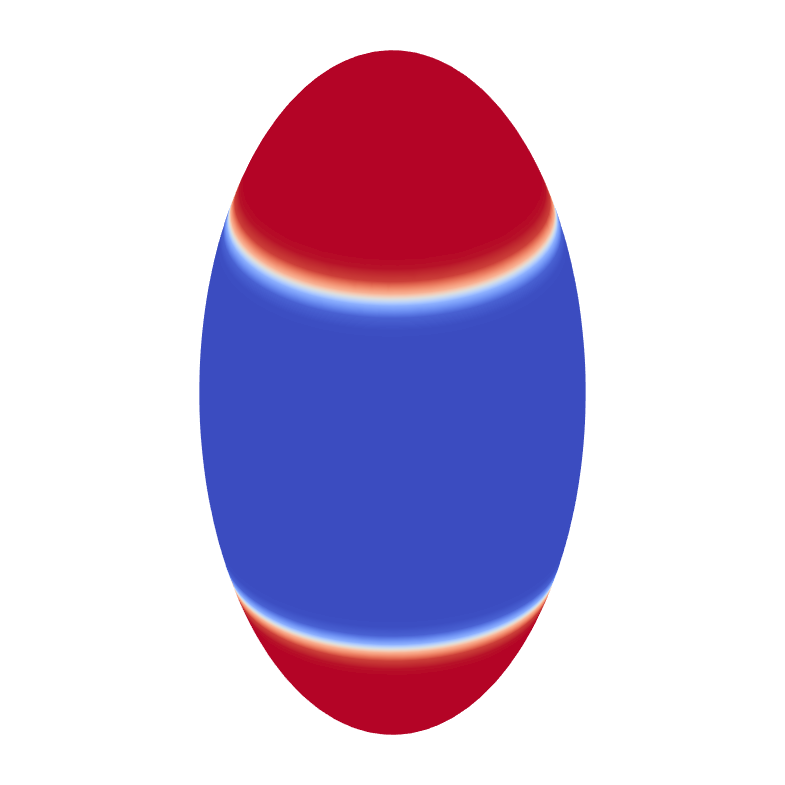
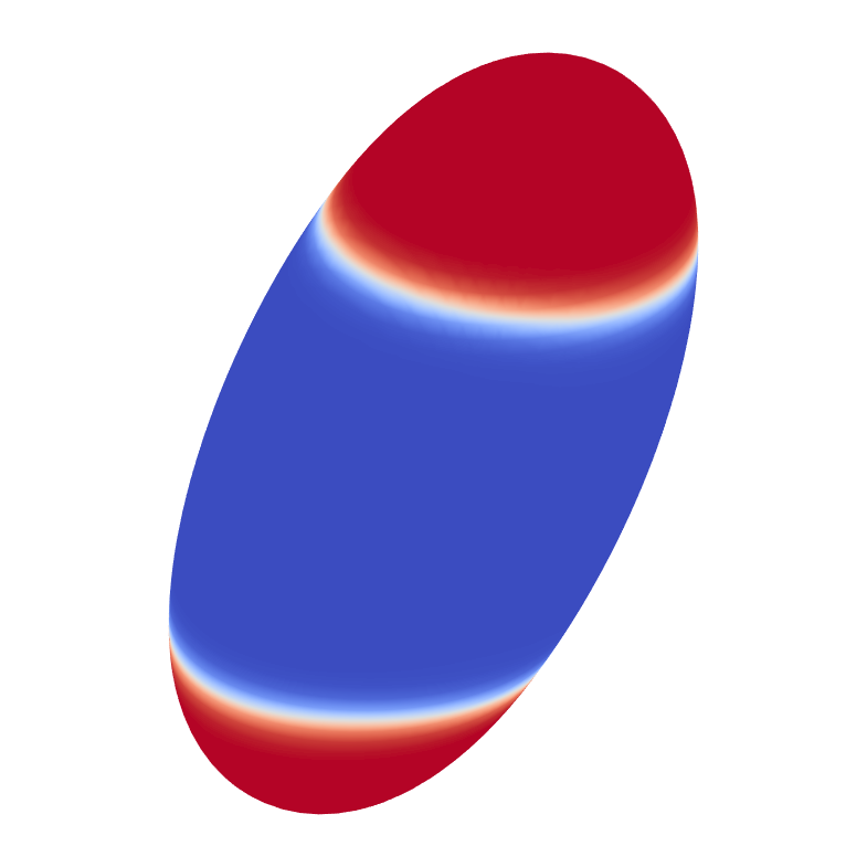
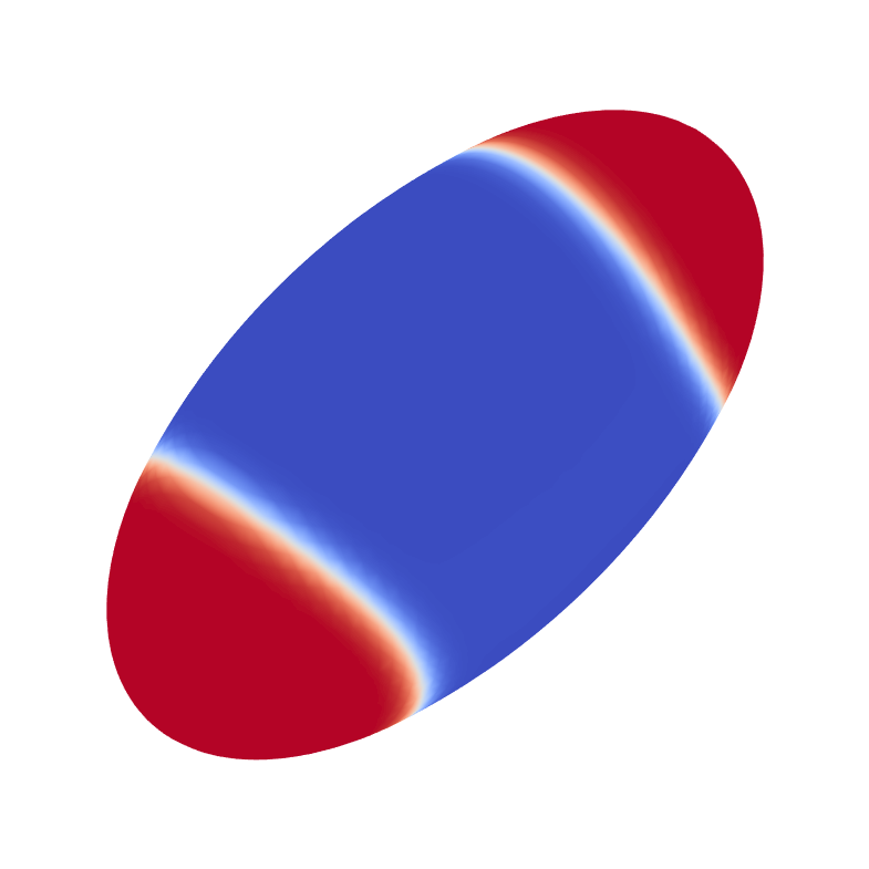
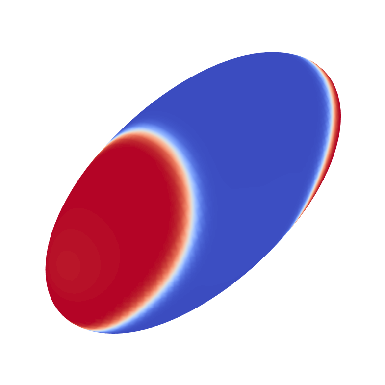
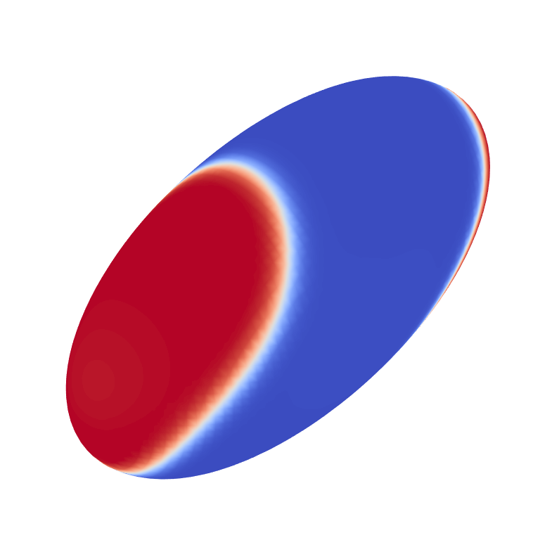
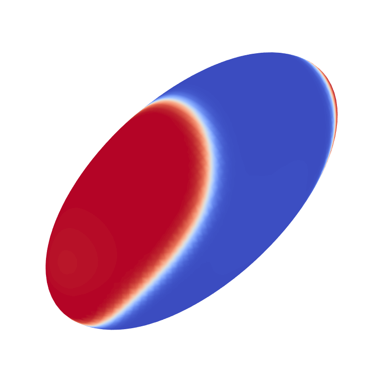
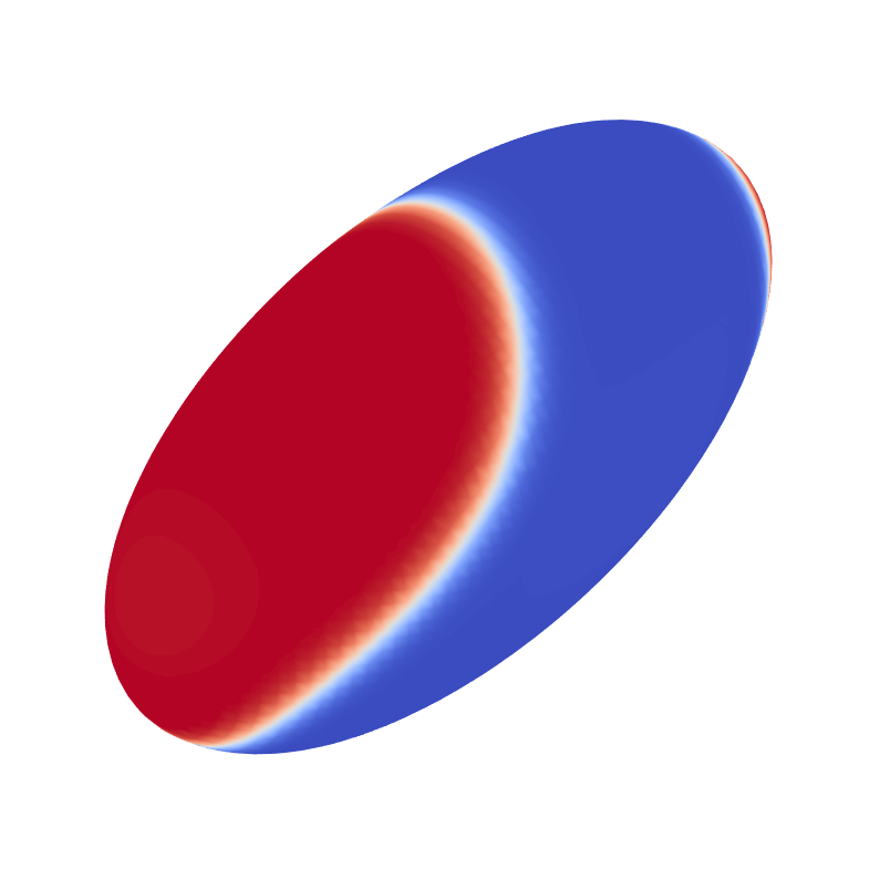
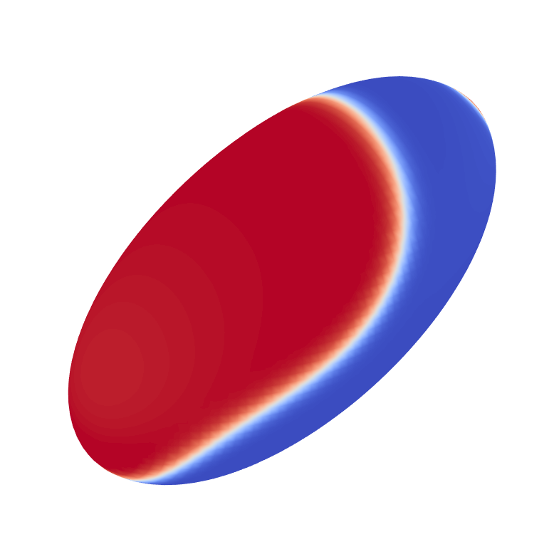
X-Y

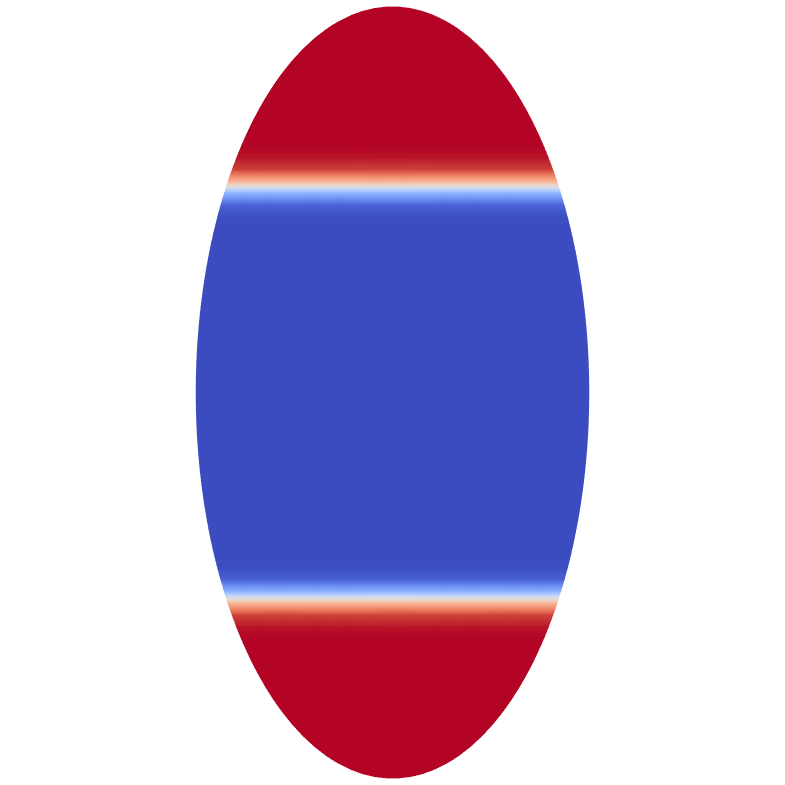
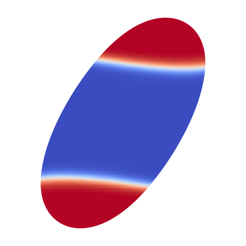
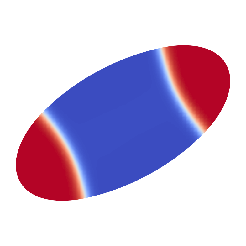
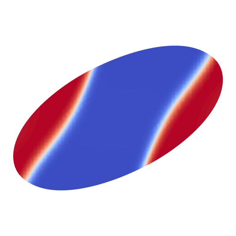
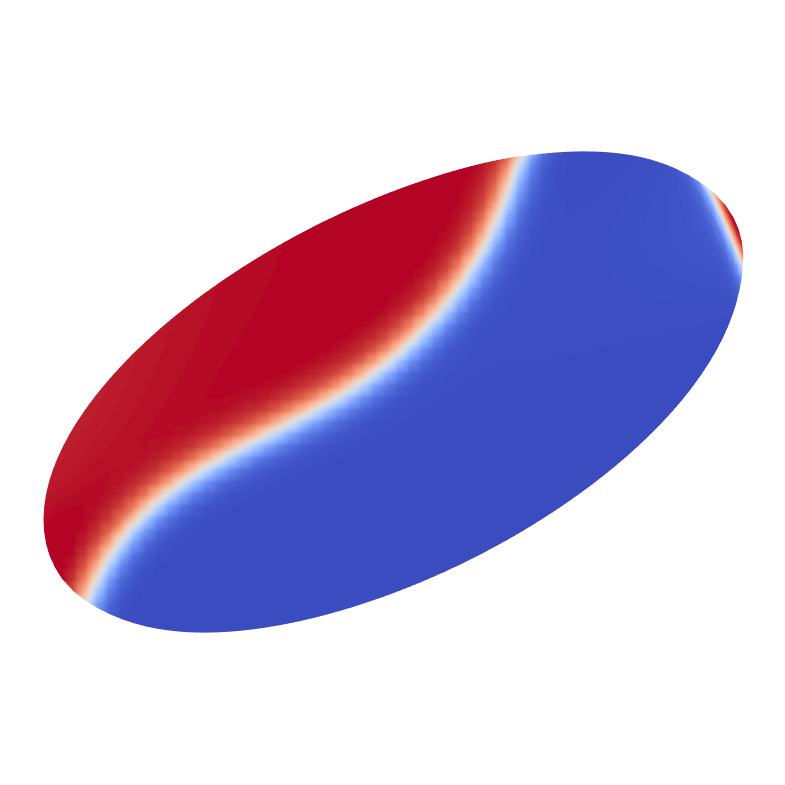
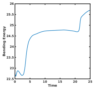
(a) Bending Energy

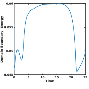
(b) Domain Boundary Energy

Figure 2: Stationary dynamics of a vesicle with $\bar{c}=0.4$ and $\alpha=20$. The soft phase has a bending rigidity of $\kappa_{c}^{B}=0.6$ and the Peclet number is $\textnormal{Pe}=0.2$. The domains remain stationary until one domain diffuses into the other.

III Results

In this section, the dynamics of a multicomponent vesicle in the presence of shear flow is examined. Unless otherwise noted, the initial shape is a prolate-ellipsoid with half-axes lengths of $0.77$, $1.51$, $0.77$ in the x-, y-, and z-directions, respectively. This results in a reduced volume of $0.9$, which measures the deviation of the volume from a perfect sphere with the same surface area. The computational domain spans $[-3,3]^{3}$ with a mesh size of $128^{3}$, while a constant time step of $5\times 10^{-3}$ is used. In a prior work the authors demonstrate qualitative convergence with these parameters Gera and Salac (2018). The computational domain is periodic in the x- and z- directions, with wall boundary conditions in the y-direction. Shear flow is applied by imposing a velocity of $\boldsymbol{u}_{bc}=(\chi\textnormal{y},0,0)$, where $\chi=1$ is the normalized shear rate, on the wall boundaries.

To remove dependence on the initial phase distribution, the initial condition for the lipid phases are assumed to be pre-segregated domains covering the tips of the vesicles. Specifically, the initial field is given by $q_{0}=((2+\textnormal{tanh}(20(y-y_{0})))+\textnormal{tanh}(-20(y+y_{0})))/2$, where $y_{0}=0.682$, which results in an average concentration of $\bar{q}=0.4$.

In all cases the Cahn number is taken to be $\textnormal{Cn}=0.05$ while the capillary bending number is fixed at $\textnormal{Ca}=20$ and the Reynolds number is $\textnormal{Re}=10^{-3}$. For simplicity, matched viscosity and density between the inner and outer fluids is assumed. As stated previously, the spontaneous curvature is zero and the two lipid domains have matched Gaussian bending rigidity. The normalized bending rigidity of the $q=0$ (hard-)phase, shown in blue below, is taken to be one, $\kappa_{c}^{A}=1$, while the bending rigidity of the $q=1$ (soft-)phase, shown in red, has a value less than one, $\kappa_{c}^{B}<1$. In most cases the surface Peclet number will vary between $\textnormal{Pe}=0.01$ and $\textnormal{Pe}=1$. Two ratios between the bending rigidity and the domain line energy are considered: $\alpha=0.5$ and $\alpha=20$. The value of $\alpha$ will be clearly stated.

The results begin with a characterization of the different dynamics observed while using the present model. The bending energy and the interfacial energy curves are shown to describe and explain the distinguishing features observed. Following this, the influence of varying bending rigidity, surface Peclet number, and domain line energy is explored.

III.1 Sample Dynamics

This section describes the spectrum of dynamics observed with the variation of the bending rigidities and surface Peclet number when a multicomponent vesicle is subjected to an external shear flow. For a single-component vesicle, matching the inner and outer fluid viscosities results in the tank-treading regime Kantsler and Steinberg (2006). When a multicomponent vesicle is exposed to shear flow, this may no longer be true as two primary competing forces exist. First, the surrounding fluid attempts to advect the phase along the vesicle membrane. As will be demonstrated, this movement results in changes in the overall energy of the vesicle. This results in the second, restorative, force: the surface diffusion of the domains to reduce the energy of the system. Varying the soft phase bending rigidity and surface Peclet number results in three different types of observed dynamics: 1) Stationary/Diffusion Dominated, 2) Vertical Banding, and 3) Phase Treading.

	Time
View	$0.0$	$2.0$	$5.0$	$10.0$	$12.5$	$15.0$	$20.0$
Iso
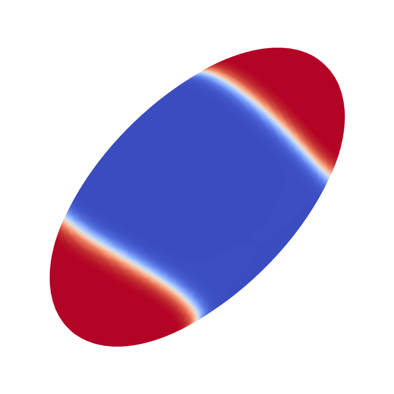
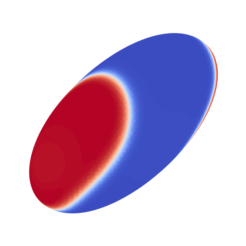
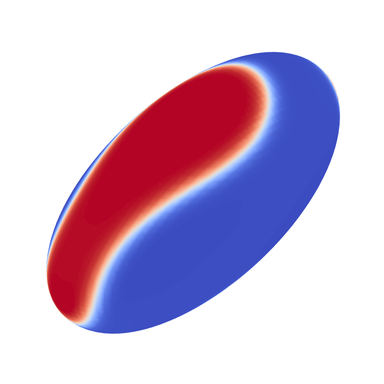
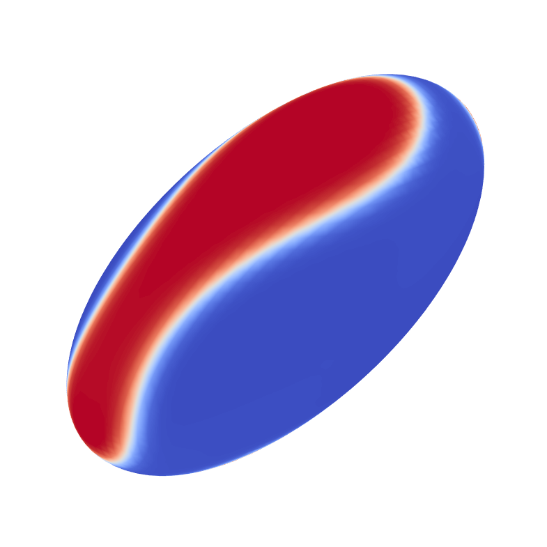
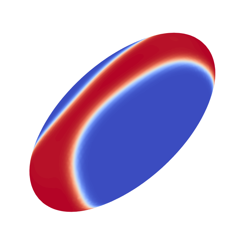
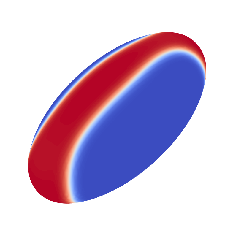
X-Y
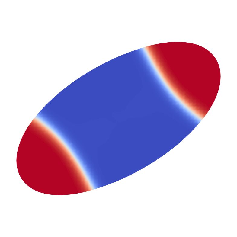
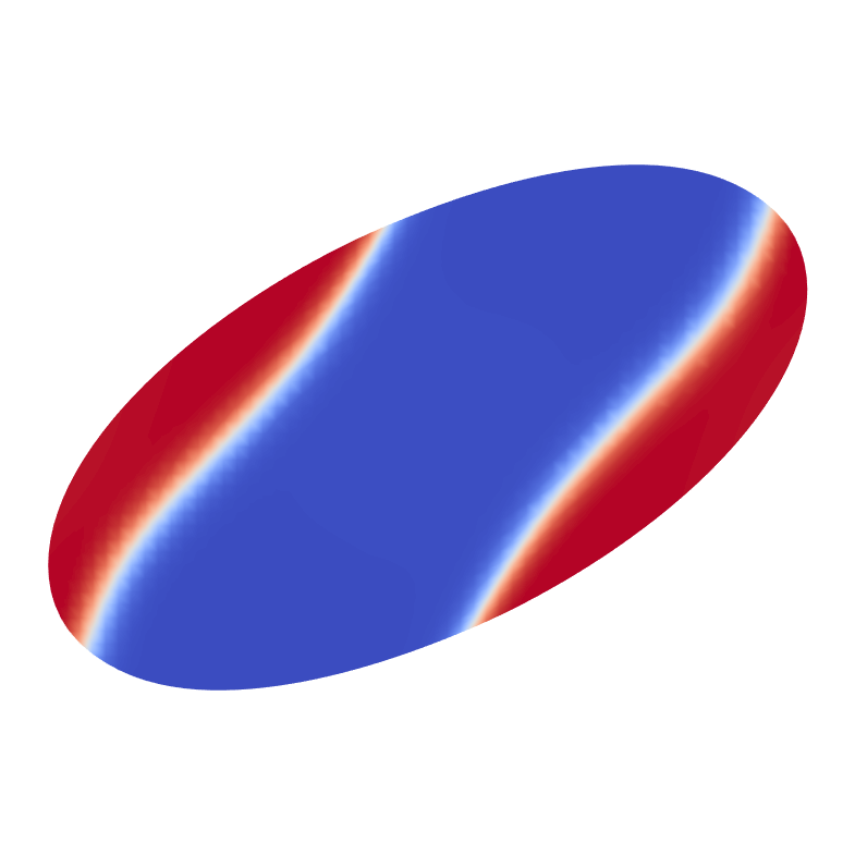
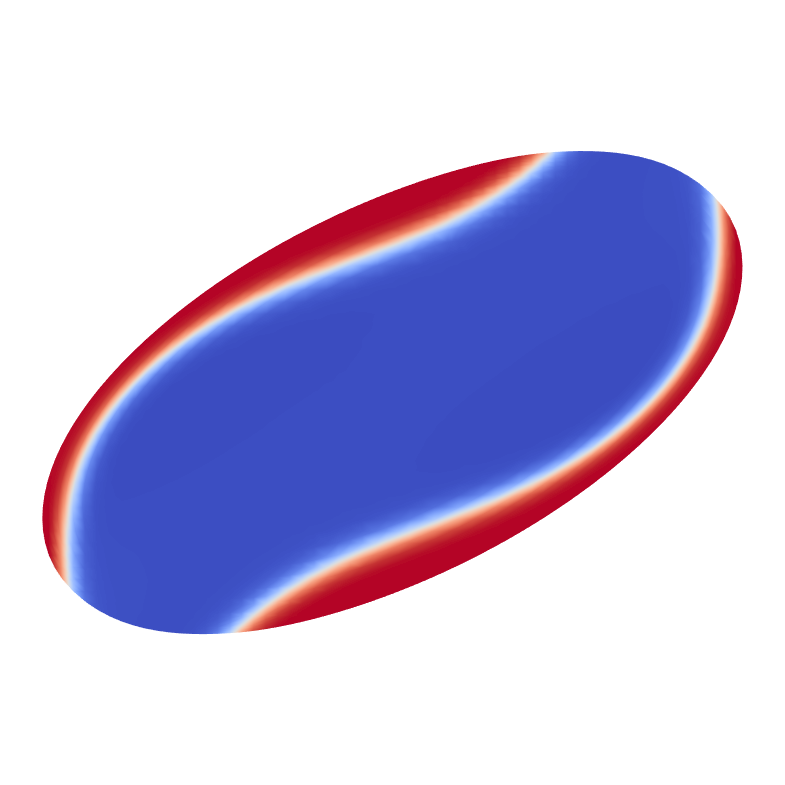
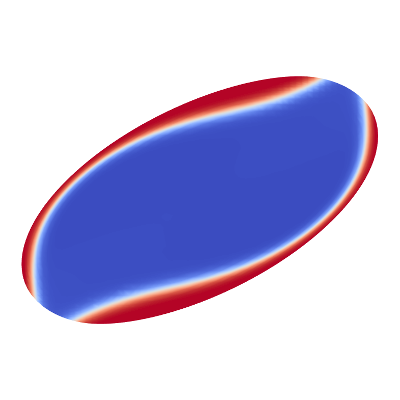
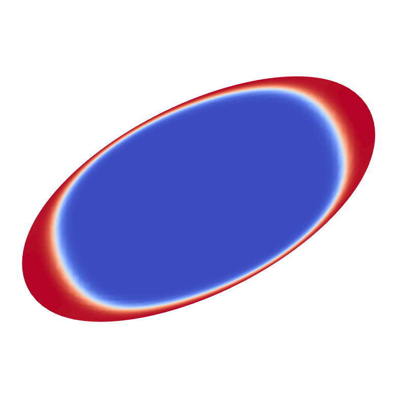
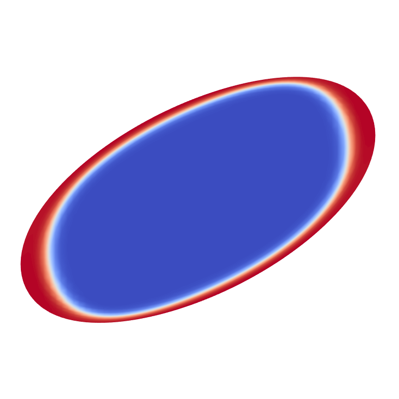
X-Z

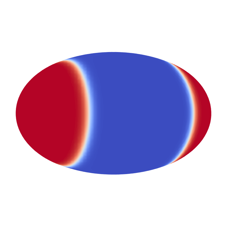
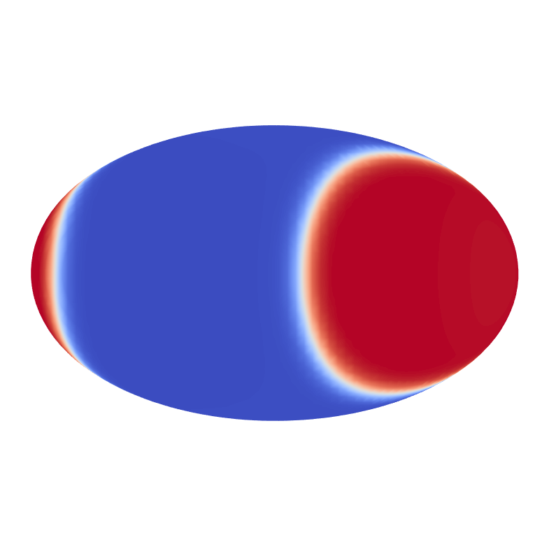
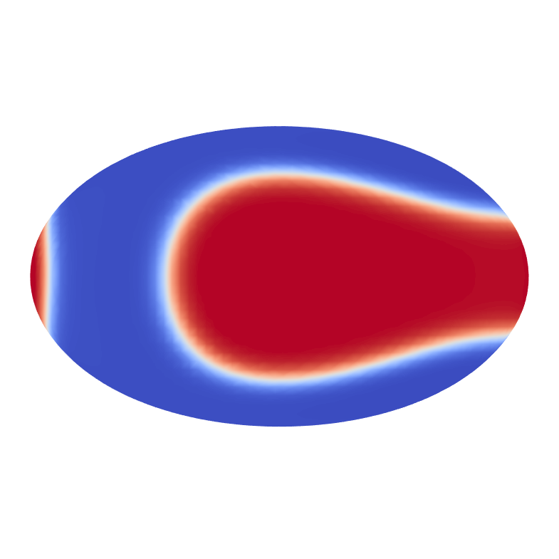
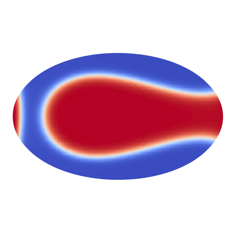
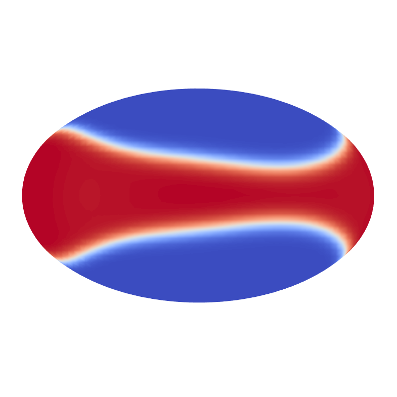
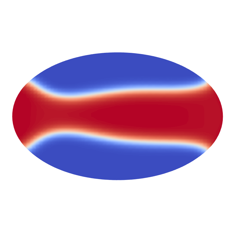
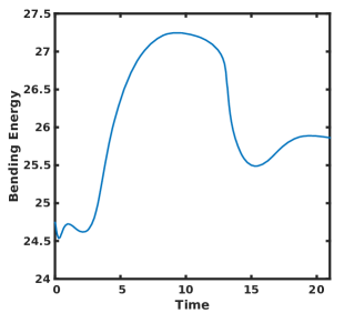
(a) Bending Energy

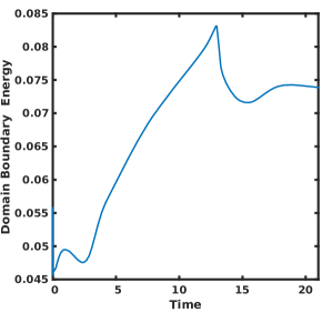
(b) Domain Boundary Energy

Figure 3: Vertical banding dynamics of a vesicle with $\bar{c}=0.4$ and $\alpha=20$. The soft phase has a bending rigidity of $\kappa_{c}^{B}=0.7$ and the Peclet number is $\textnormal{Pe}=0.5$. The higher Peclet number allows for the domains to extend and eventually merge.

III.1.1 Stationary/Diffusion Dominated Dynamics

Recall that the surface Peclet number indicates how quickly the surface phases can adjust to changes in the system energy; smaller values of Pe indicate the surface phases can adjust quickly relative to the advection forces. Alternatively, decreasing the bending rigidity of the soft phase decreases the overall energy when the soft phase inhabits the high curvature regions of the vesicle. For small values of Pe and $\kappa_{c}^{B}$, it has been observed that the domains remain at the vesicle tips until one domain grows at the expense of the other (which is typical of Cahn-Hilliard models). This type of dynamic is denoted as stationary or diffusion dominated, and has been previously seen for two-dimensional multicomponent vesicles Liu et al. (2017).

For example, consider a vesicle where the soft-phase bending rigidity is given by $\kappa_{c}^{B}=0.6$ with a Peclet number of $\textnormal{Pe}=0.2$, Fig 2. Until a time of $t=2.5$ very little deformation of the domains is observed as the vesicle reaches the equilibrium inclination angle. From a time of $t=2.5$ to $t=5$, the domains deform until reaching an equilibrium, elongated shape. They remain in this shape until a time of $t=15$, after which one domain grows at the expense of the other domain.

This dynamic is confirmed by considering the bending and domain boundary energy, Fig 2. Initially, there is growth in the bending and domain boundary energy as the domains on the surface of the vesicle change from circular to slight elongated. Both energies remain relatively constant, until one of the domains grows dramatically to reduce the domain boundary energy. This merging event results in a larger bending energy, as a smaller amount of the softer phase is in the high curvature tips. After reaching the minima, there is a slight increase in domain boundary and bending energy as the domains slightly elongate, and a major portion of it lies on the low curvature region of the vesicle. Similar dynamics have been observed in the recent two-dimensional work of Liu et al. Liu et al. (2017).

	Time
View	$0.0$	$0.5$	$9.0$	$13.0$	$15.0$	$17.0$	$18.0$	$20.0$
Iso
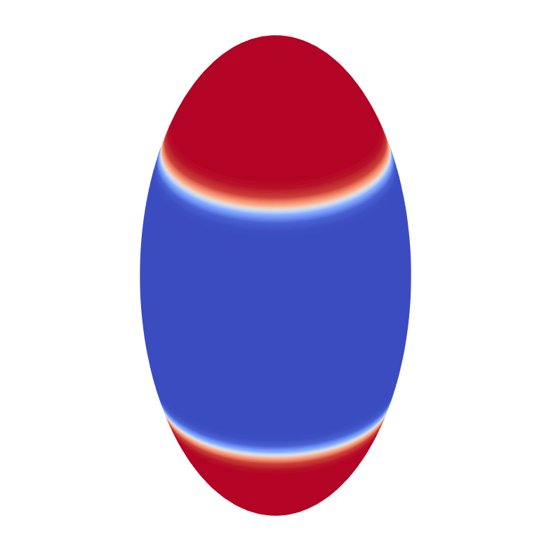
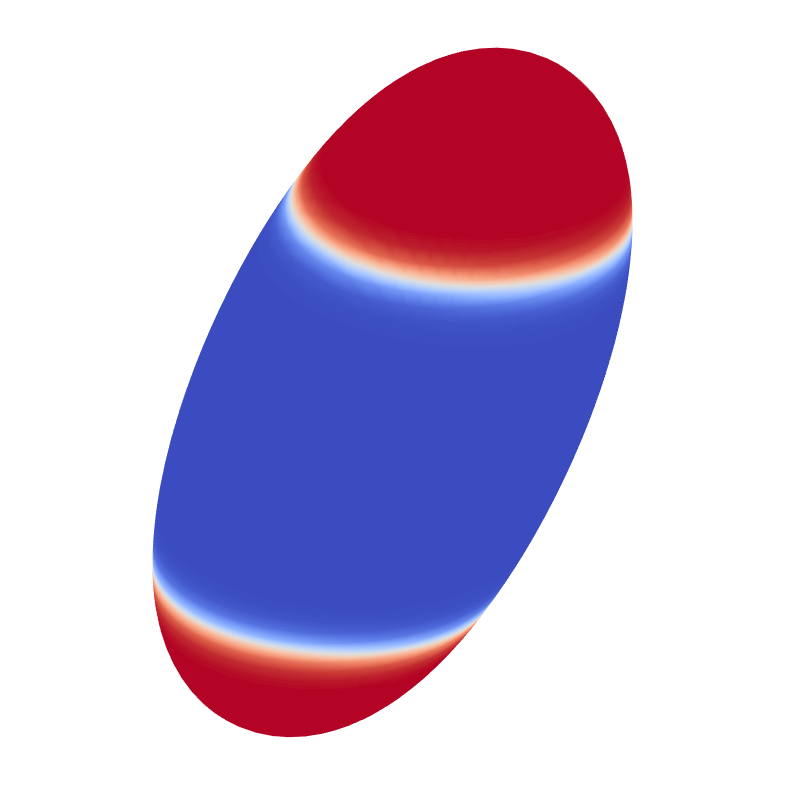
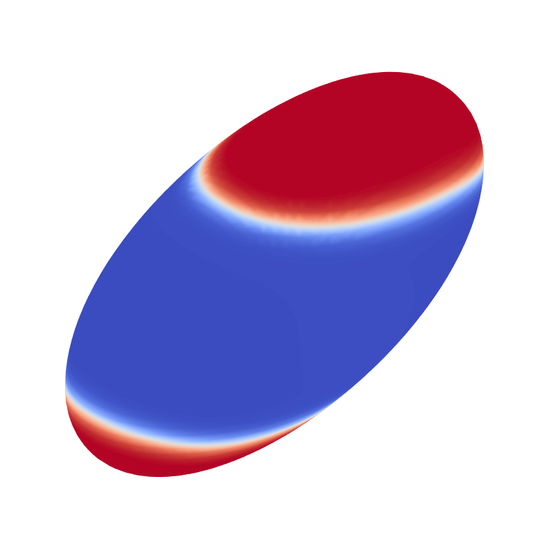
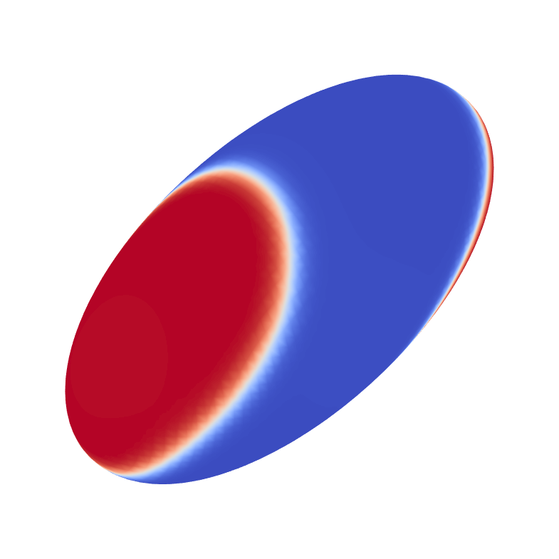
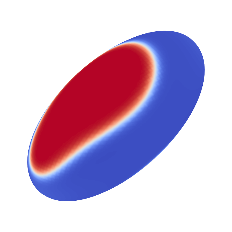
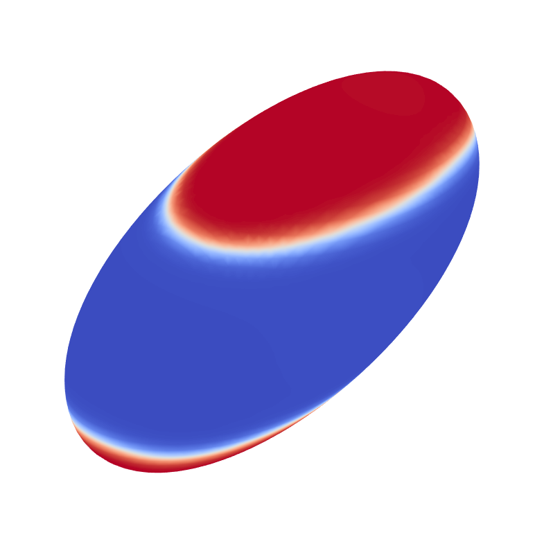
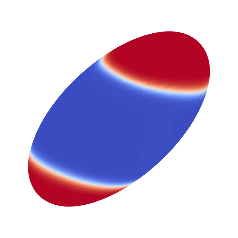
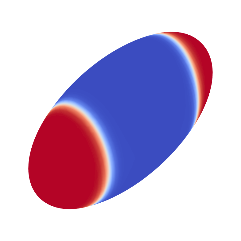
X-Y

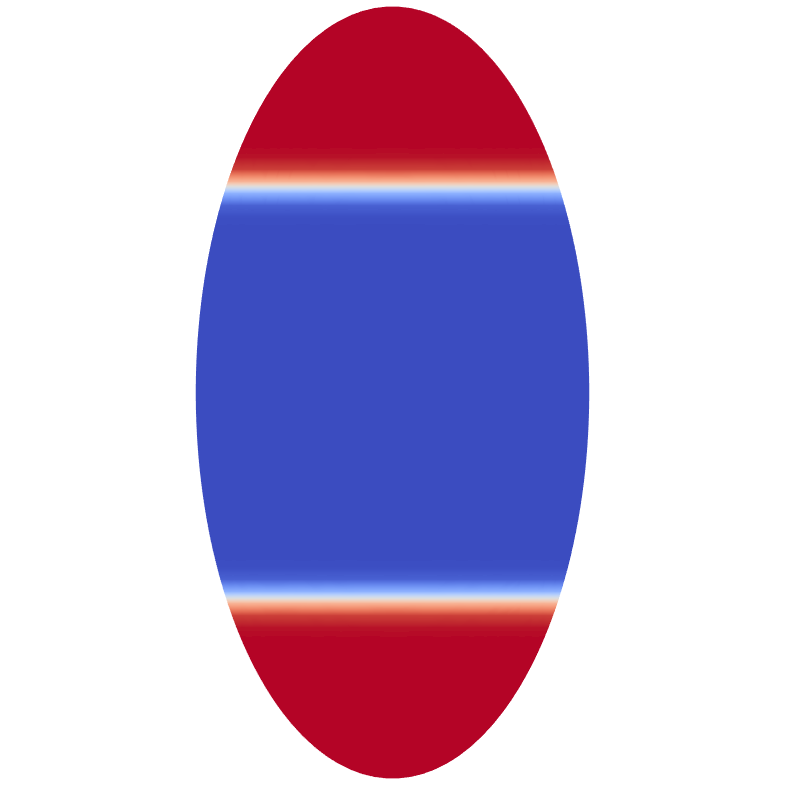
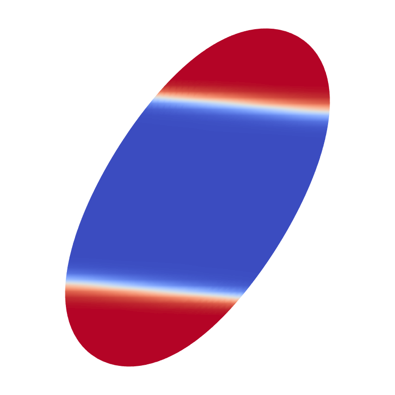
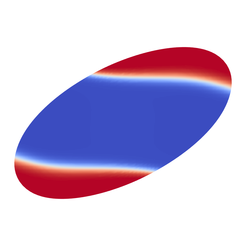
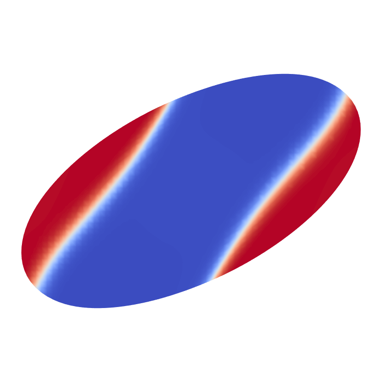
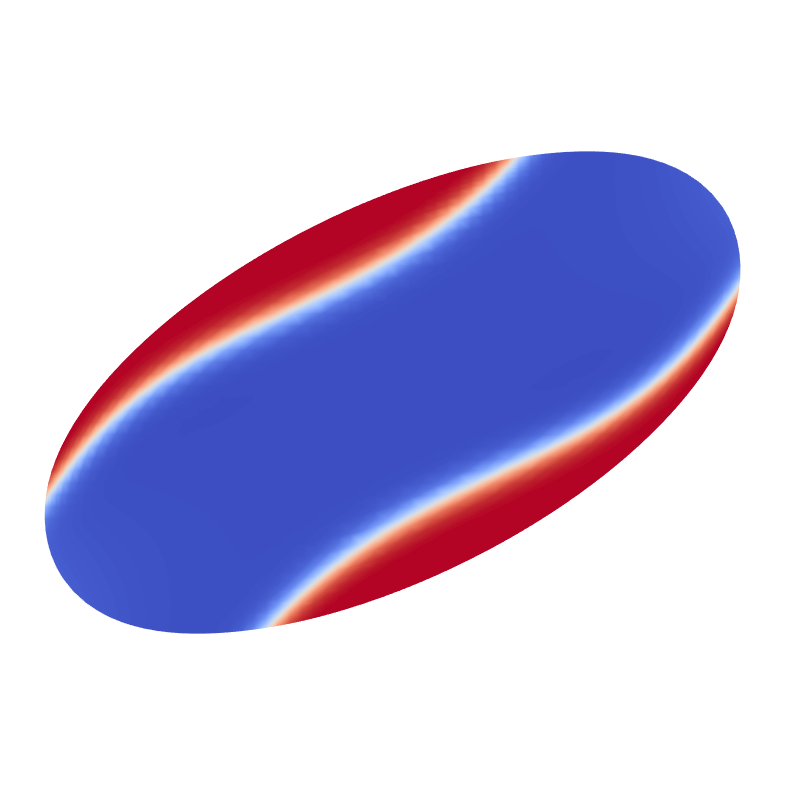
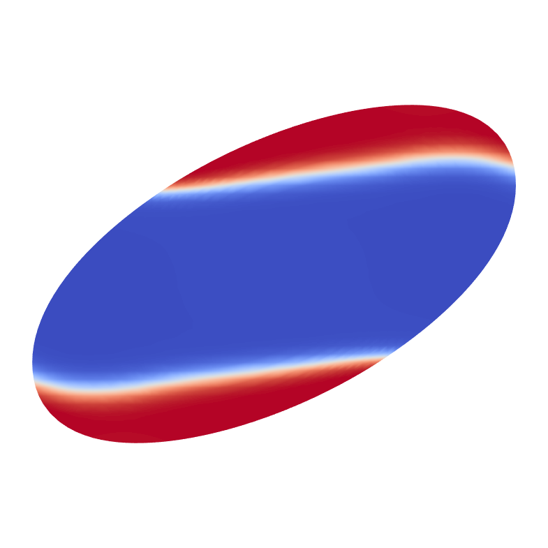
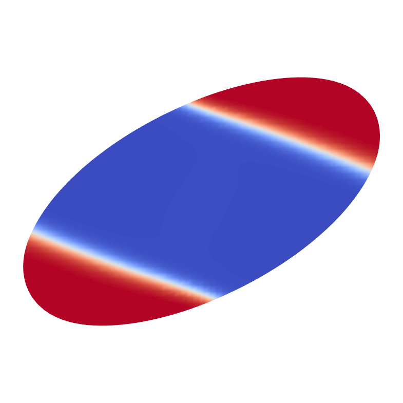
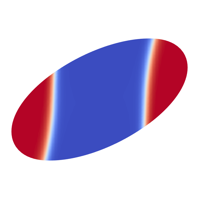
(a) Bending Energy

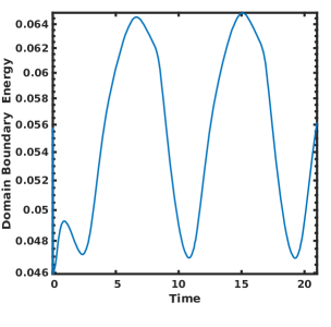
(b) Domain Boundary Energy

Figure 4: Phase treading dynamics of a vesicle with $\bar{c}=0.4$ and $\alpha=20$. The soft phase has a bending rigidity of $\kappa_{c}^{B}=0.8$ and the Peclet number is $\textnormal{Pe}=1.0$. The Peclet number allows for the domains to tread along the membrane.

III.1.2 Vertical Stationary Band Dynamics

When the Peclet number and soft phase rigidity are increased, the vertical stationary banding dynamic is observed. The vertical stationary dynamic is characterized by the stretching of the domains from the tips vertically on the surface, with the eventual merging of the domain resulting in a single and thin domain.

Consider a vesicle with $\textnormal{Pe}=0.5$ and soft phase bending rigidity of $\kappa_{c}^{B}=0.7$, Fig. 3. As in the diffusion dominated case shown previously, the vesicle rotates and achieves a relatively stable inclination and the domains begin to elongate. Due to the higher Peclet number, fluid motion forces the domains to elongate further along the vesicle membrane than in the prior case. This elongation continues until the two domains meet and merge into a single domain spanning the vertical plane.

Exploration of the bending and domain boundary energy provides further insights to this dynamic. As the domains begin to grow along the vesicle, both energies increase until $t=12.5$. At this point the two domains merge and there is a large decrease in the domain boundary energy. The bending energy decreases more slowly, as a large amount of the softer phase still inhabits the low curvature regions away from the tips. Eventually the soft phase diffuses to the tips, resulting in a further reduction of the bending energy. After reaching the minima, there is a slight increase in the bending and domain boundary energy. This is due to some material being advected from the high curvature tips to the lower curvature center. Note that this particular dynamic has not been previously reported.

III.1.3 Phase Treading Dynamics

Further increasing the Peclet or soft phase bending rigidity decreases the restorative surface diffusion forces, which allows the force exerted by the external fluid to become dominate. An example of this behavior can be seen in Fig. 4, where the soft phase has a bending rigidity of $\kappa_{c}^{B}=0.8$ and the Peclet number is $\textnormal{Pe}=1.0$. As in the prior examples, the vesicle rotates to become more aligned with the shear flow. During this time the domains elongate along the long-axis. Unlike the prior cases, the domains do not remain attached to the vesicle tips and migrate along the interface until it reaches the other tip, when the process is then repeated. Similar dynamics have been observed in the recent two-dimensional work of Liu et al. Liu et al. (2017).

The periodic nature of this dynamic can be seen by considering the bending and domain boundary energy, Fig. 4. After an initially transient period, both the bending and domain boundary energy quickly increase as the domains leave the tips. When the domains reach the opposite tip, both energies quickly decrease, with the decrease in the domain boundary energy slightly lagging the drop in the bending energy.

	Time
View	$0.5$	$2.0$	$4.0$	$6.0$	$10.0$	$14.0$	$16.0$	$20.0$
Iso
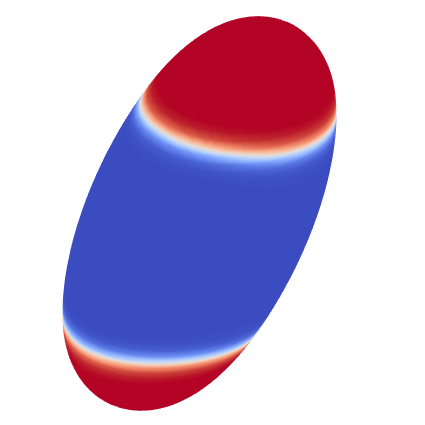
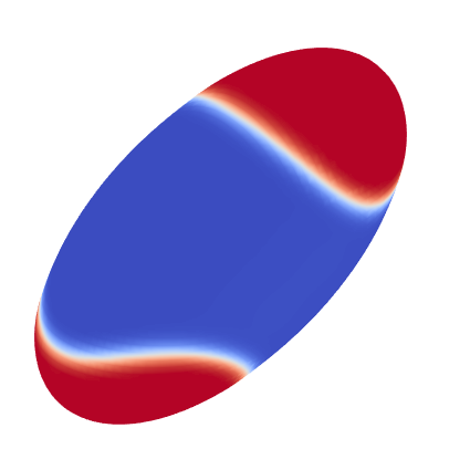
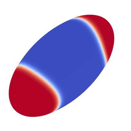
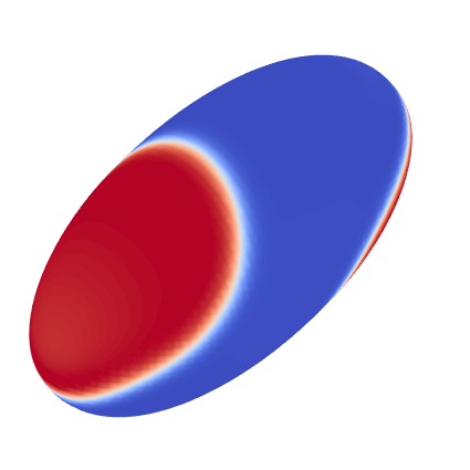
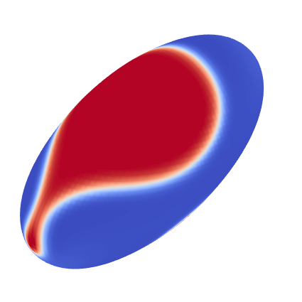
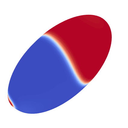
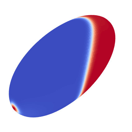
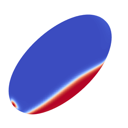
X-Y

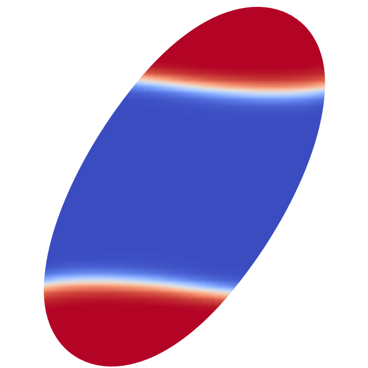
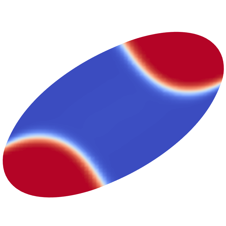
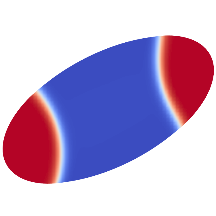
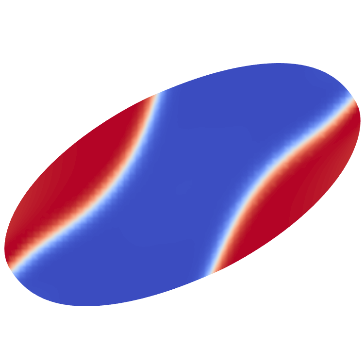
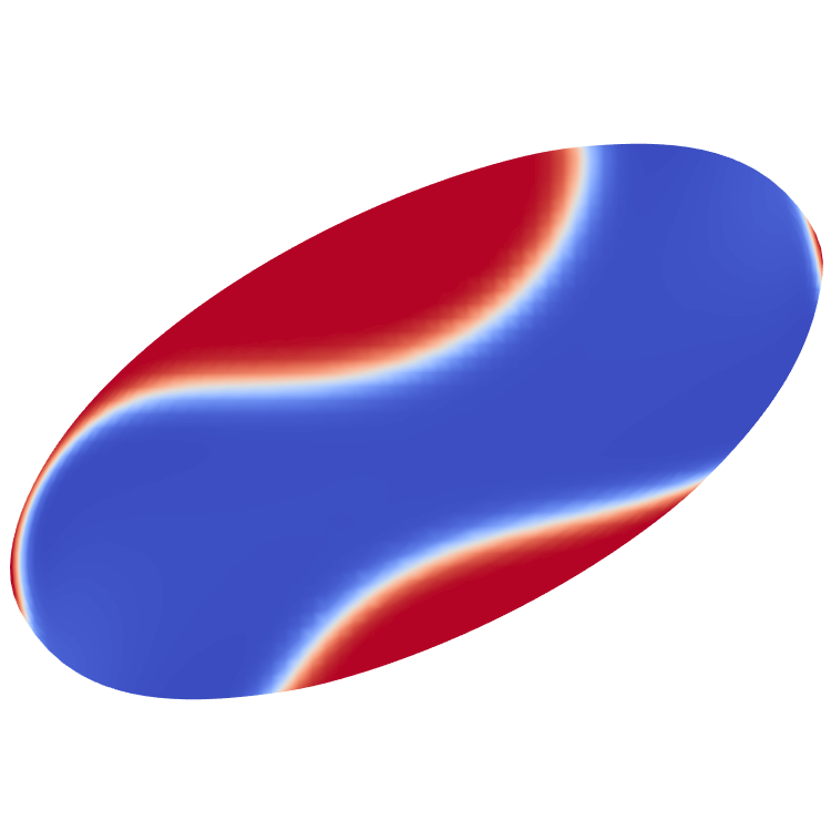
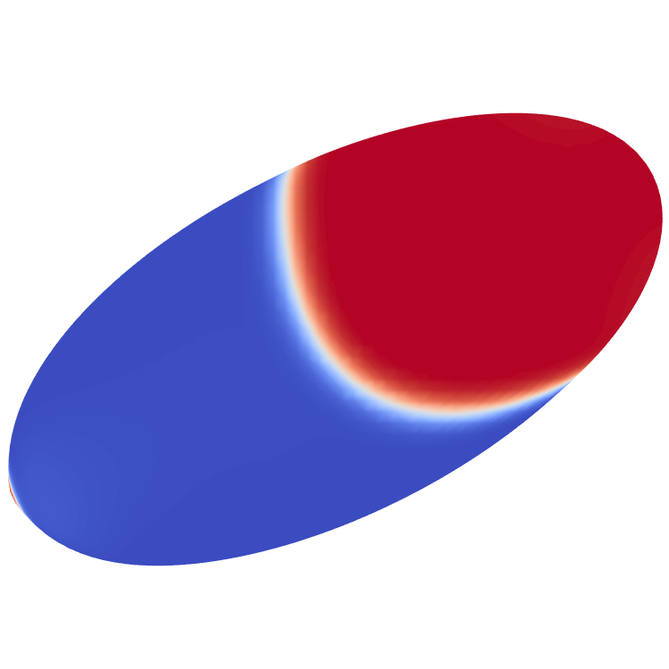
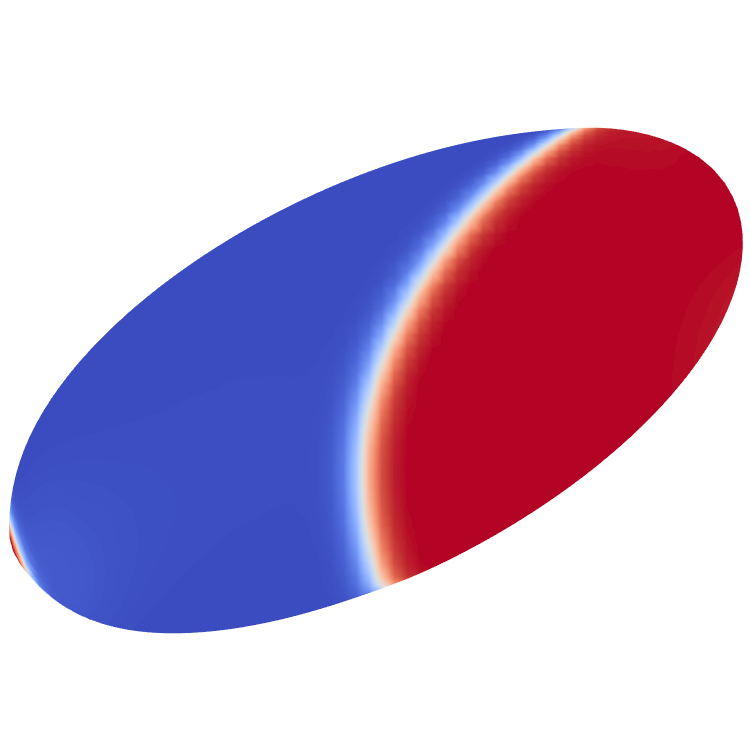
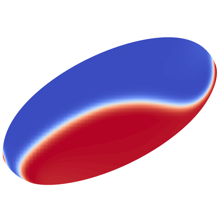
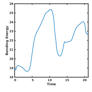
(a) Bending Energy

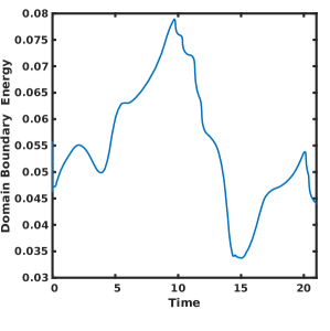
(b) Domain Boundary Energy

Figure 5: Sample of the Tread-1 dynamic for a vesicle with $\bar{c}=0.4$ and $\alpha=20$. A softer phase with a bending rigidity of $\kappa_{c}^{B}=0.4$ and with a Peclet number of $\textnormal{Pe}=0.3$ results in the treading of domains for a certain time before one of the domains grows at the expense of the other domain.

Tread-n Dynamics:

An interesting sub-dynamic of phase treading exists when the surface Peclet number or soft phase bending rigidity are too large to allow for stationary phases or vertical banding, but not large enough to allow for long-term phase treading behavior. In this work, this sub-dynamic is further classified as Tread-n, where $n$ indicates the number of times that each phase travels from one tip to the other tip before diffusion dominates and results in a single, large domain.

For example, consider the dynamics with a Peclet number of $\textnormal{Pe}=0.3$ and a soft phase bending rigidity of $\kappa_{c}^{B}=0.4$, Fig. 5. As shown before, the vesicle begins to align itself with the shear flow and the phases begin to migrate along the vesicle membrane. During this migration, the upper domain grows at the expense of the lower phase. Once the upper domain reaches the opposite tip, the lower domain has completely disappeared. This is further confirmed via the energy curves, Fig. 5. It is clear that a large decrease in the domain boundary energy occurs between a time of $t=10$ and $t=15$, which corresponds to the domain merging event. As the domains only switched tips once, this dynamic would be classified as Tread-1. Note that the small soft phase seen in Fig. 5 is typical of this dynamic, as the advective forces are not strong enough to completely overcome all of the surface diffusion restorative forces. This is further discussed in later sections.

III.2 Dynamics as a function of $\kappa_{c}^{B}$ and Pe

From the prior results, it is clear that the dynamics of the vesicle strongly depend on both the soft phase bending rigidity and the surface Peclet number. In this section, systematic parameter studies investigating the dynamics for a pre-segregated and multicomponent vesicle with an average concentration of $\bar{c}=0.4$ as a function of $\kappa_{c}^{B}$ and Pe for two characteristic domain line energies are performed. In both cases, the dynamics will be reported via phase diagrams.

III.2.1 Domain Line Tension of $\alpha=20$

Figure 6: Variation of vesicle behavior with Peclet number and bending rigidity of the soft phase for $\bar{c}=0.4$ and $\alpha=20$.

	Time
$\kappa_{c}^{B}$	$5.0$	$9.0$	$10.0$	$12.5$	$15.0$	$17.5$	$20.0$	$20.5$
0.5
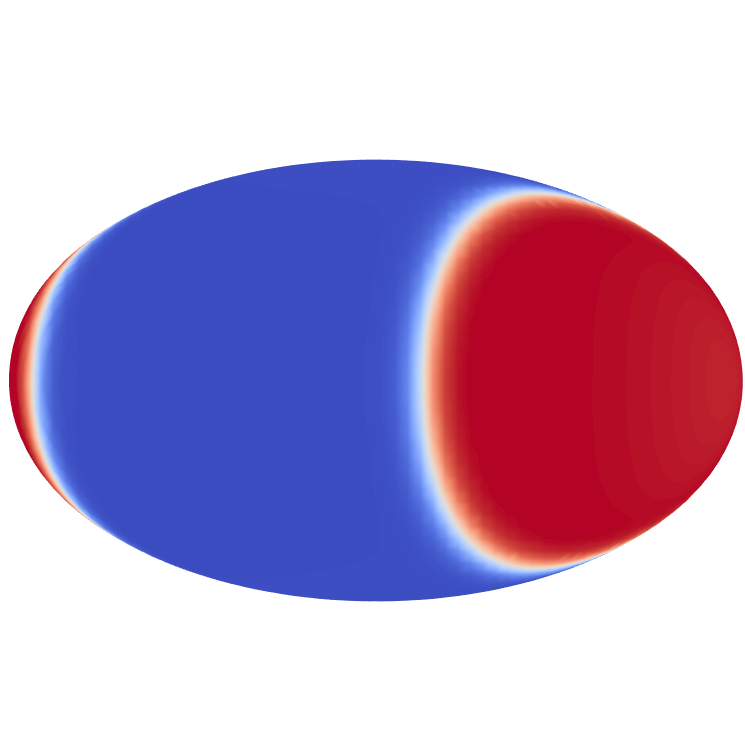
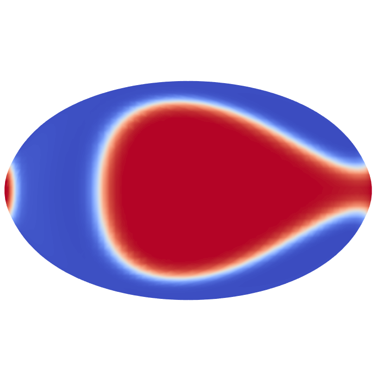
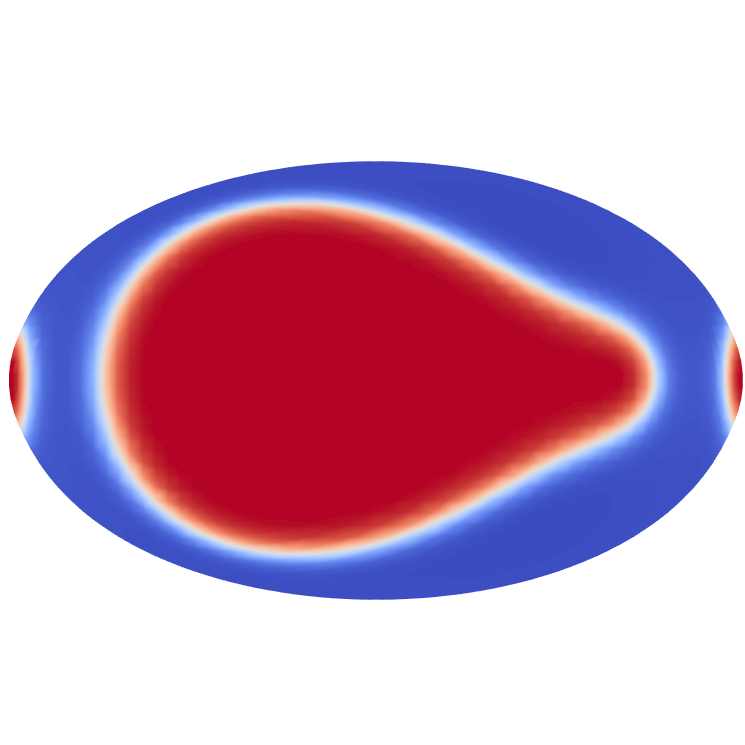
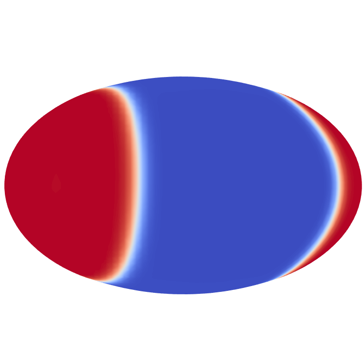
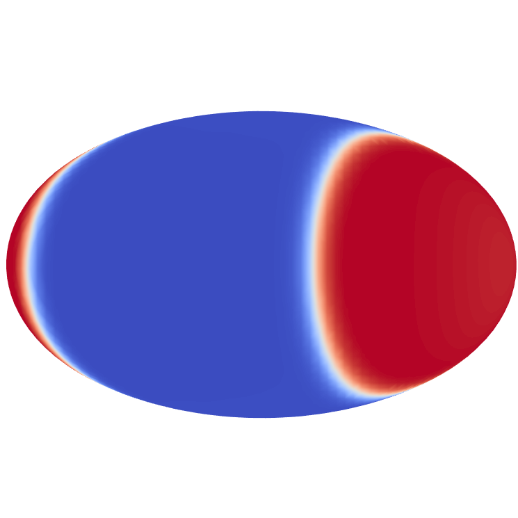
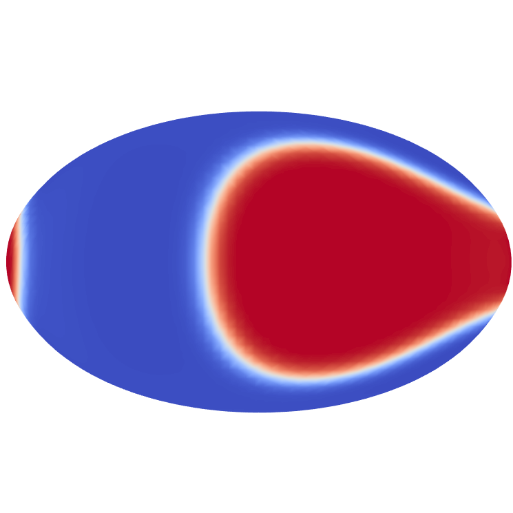
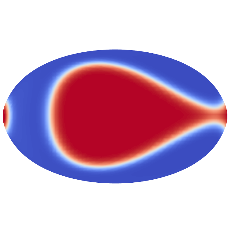
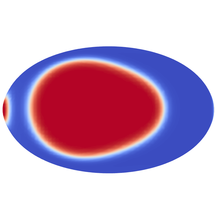
0.7

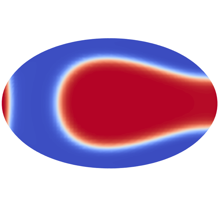
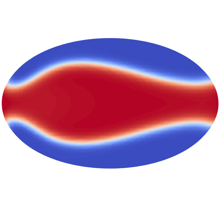
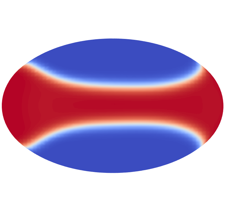
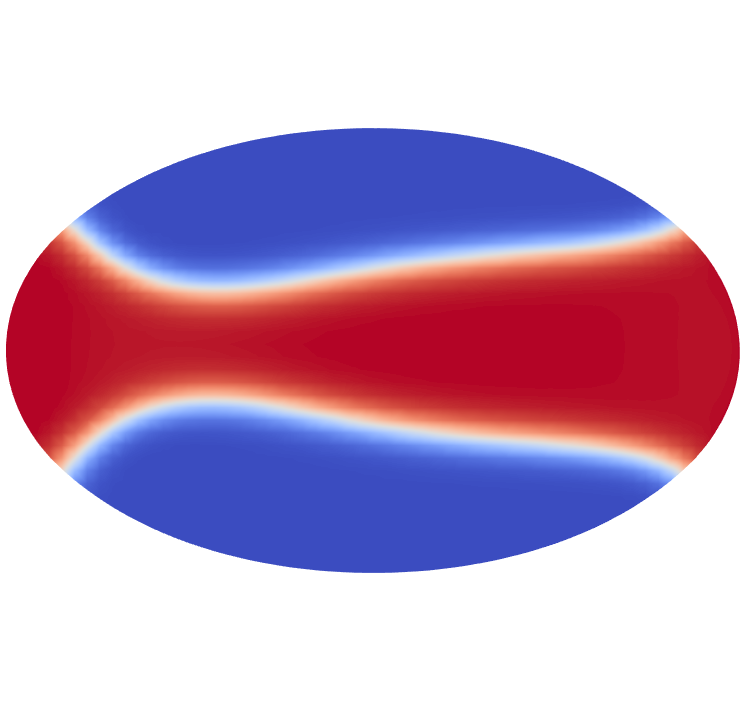
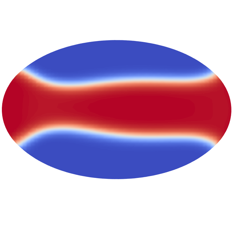
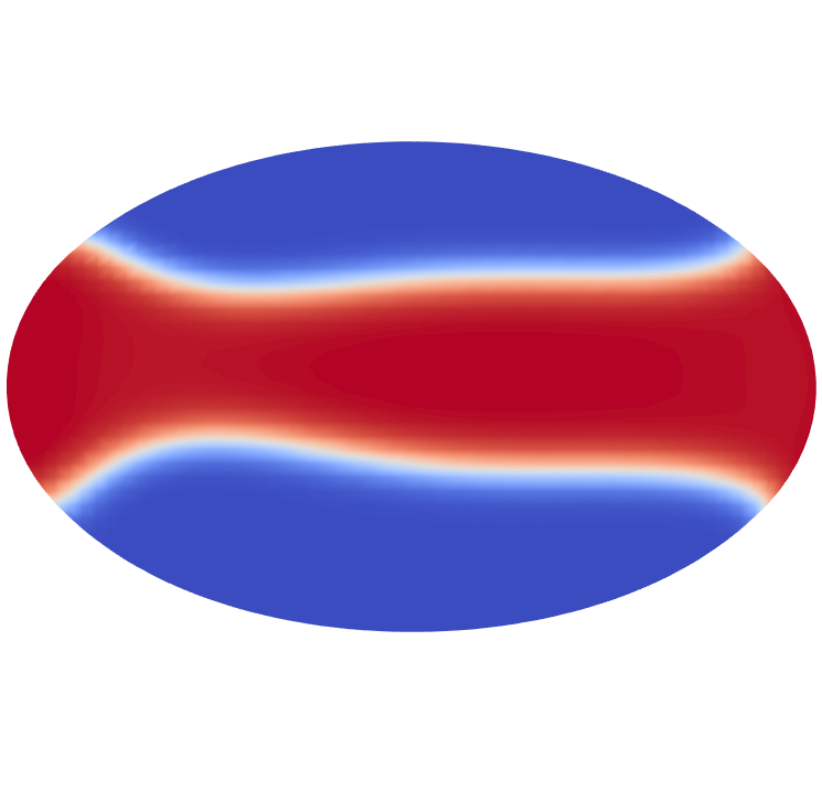
Figure 7: Treading dynamics of lipids on the vesicle in X-Z plane for $\bar{c}=0.4$, $\alpha=20$, and $\textnormal{Pe}=0.5$. Two soft phase bending rigidities are shown.

First consider the phase diagram for $\alpha=20$, Fig. 6. This diagram clearly shows the three regimes demonstrated previously: stationary phase, vertical banding, and phase treading. As has been previously demonstrated for two-dimensional vesicles, there is a linear relationship between the critical shear rate needed for phase treading and the bending rigidity of the soft phase Liu et al. (2017). The surface Peclet number scales with the shear rate, i.e. as the shear rate increases so does Pe. Therefore, it should be expected that as the bending rigidity for the soft phase decreases, the critical Peclet number needed for the stationary phase/treading phase should increase. As can be seen in the phase diagram, this is not the case. For example, a multicomponent vesicle with $\kappa_{c}^{B}=0.7$ and $\textnormal{Pe}=0.5$ is in the vertical banding regime while one with $\kappa_{c}^{B}=0.5$ and $\textnormal{Pe}=0.5$ is in the phase treading regime. To explain this counter-intuitive behavior, compare the dynamics between $\kappa_{c}^{B}=0.5$ and $\kappa_{c}^{B}=0.7$ for $\textnormal{Pe}=0.5$, Fig. 7. In general, the domains with $\kappa_{c}^{B}=0.7$ are thinner at the leading edge and thicker at the tail compared to the domains with $\kappa_{c}^{B}=0.5$, see the domains at a time of $t=9$ for an example. As the tails for $\kappa_{c}^{B}=0.7$ are thicker, the domains can extend further along the vesicle and still maintain contact with the vesicle tips. This allows for the domains to extend and eventually merge, forming a single, thin domain. In contrast, the thin tail for $\kappa_{c}^{B}=0.5$ results in the eventual pinch-off of the domains, which allows for continued phase-treading.

The rationale for this behavior can be seen by considering the curvature on the vesicle membrane at a time of $t=9$, Fig. 8. As can be seen, due to the deformation of the vesicle in shear flow, the membrane has a higher curvature along the horizontal edges of the vesicle than along the vertical edges. A higher curvature along the horizontal edges of the vesicle is true in general, and only the particular curvature values depend on the bending rigidity of the soft phase. When the soft phase bending rigidity is $\kappa_{c}^{B}=0.5$, material is drawn towards these high curvature regions on the edge. As the domain grows towards the edge, the material required is taken from the tail, which results in a thin tail. On the other hand, when $\kappa_{c}^{B}=0.7$, the force drawing the soft phase down towards the edge is small, which allows it to maintain a thick tail and thus contact with the vesicle tip.

(a) X-Z plane

(b) X-Y plane

Figure 8: Curvature on the vesicle shown in Fig. 7. Red (color online) indicates regions of high curvature. In this figure $\kappa_{c}^{B}=0.5$.

	Time
View	$4.0$	$6.0$	$10.0$	$12.5$	$14.0$	$16.0$	$20.0$	$22.5$	$25.0$	$30.0$	$35.0$
Iso
X-Y

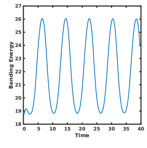
(a) Bending Energy

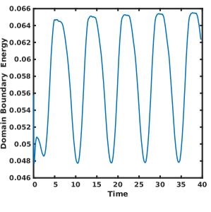
(b) Domain Boundary Energy

Figure 9: Dynamics of lipids on the vesicle for $\bar{c}=0.4$ and $\alpha=20$. The softer phase has a bending rigidity of $\kappa_{c}^{B}=0.4$ and with a Peclet number of $\textnormal{Pe}=20.0$ results in treading of domains.

The small domains seen at the vesicle tips, such as those shown in Fig. 5, can also be explained by considering the membrane curvature. The highest curvature regions occur at the membrane tips, Fig. 8, and to reduce the overall bending energy, the soft phase will preferentially aggregate in these regions if possible. This aggregation will occur when either bending rigidity of the soft phase, $\kappa_{c}^{B}$, or the surface Peclet number, Pe are small. This can be seen in Fig. (5) where $\kappa_{c}^{B}=0.4$, however as it increases to $\kappa_{c}^{B}=0.8$, the domains on the tips are no longer observed, Fig. (4).

The influence of Pe on this behavior is verified by considering the result with a larger Peclet number, $\textnormal{Pe}=20$, as seen in Fig. 9. While the soft phase bending rigidity is the same as before, $\kappa_{c}^{B}=0.4$, these small domains are no longer present. Additionally, due to the slower surface diffusion, the merging even occurs much later. This is shown by the periodic nature of the bending and domain boundary energy for the $\textnormal{Pe}=20$ case, Fig. 9, which still has not merged at a time of $t=40$.

III.2.2 Domain Line Tension of $\alpha=0.5$

Now consider the dynamics for $\alpha=0.5$. In this case, the domain line forces is stronger than the bending forces. Performing a systematic parameter study, the resulting phase diagram can be seen in Fig. 10. It is interesting to note that in this case only two dynamics are observed: stationary phases and phase treading. Compared to the $\alpha=20$ situation shown previously, the contribution of the domain line energy to the dynamics is 40-times larger, and thus the system will attempt to minimize the total domain boundary length. It is therefore not possible with $\alpha=0.5$ to obtain the vertical banding dynamic seen previously. Additionally, it is important to understand the influence of $\alpha$ on the evolution of the surface domains and the fluid field, Eqs. (17) and (21). When $\alpha=0.5$, the influence of the bending rigidity difference on the diffusion of the surface phases becomes weak, while the influence of the variation of the surface phases on the fluid field becomes strong. Therefore, it should be expected that the influence of the bending rigidity difference as a function of surface Peclet number should be decreased; which is what is observed in the phase diagram seen in Fig. 10.

A sample result with $\alpha=0.5$, $\kappa_{c}^{B}=0.4$ and $\textnormal{Pe}=0.3$ is seen in Figs. 11-14. The results of Fig. 11 are centered on the vesicle, while those in Fig. 12 demonstrate the motion induced after symmetry breaking.

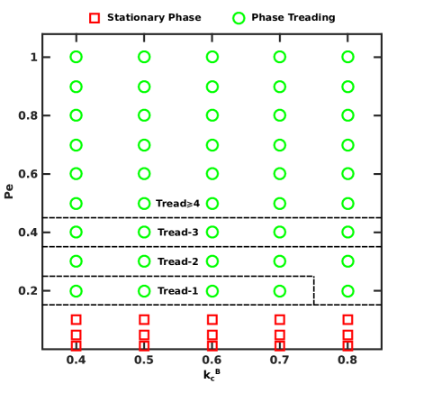
Figure 10: Variation of vesicle behavior with Peclet number and bending rigidity of the soft phase for $\bar{c}=0.4$ and $\alpha=0.5$.

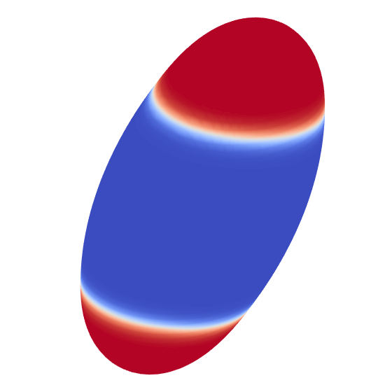
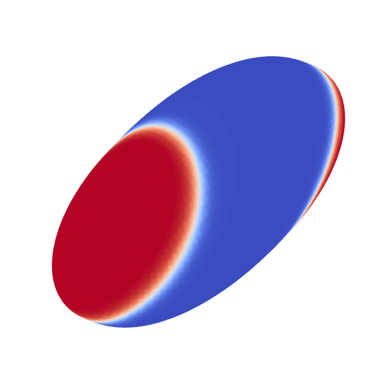
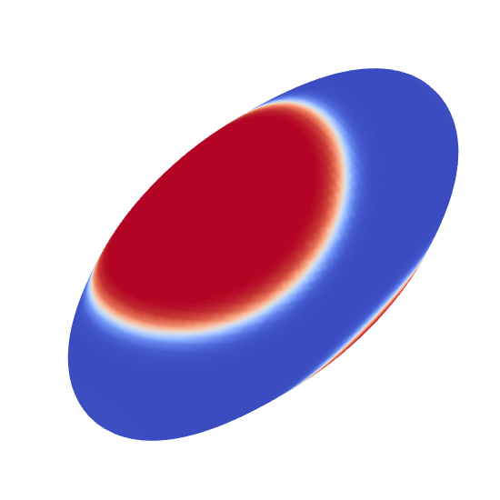
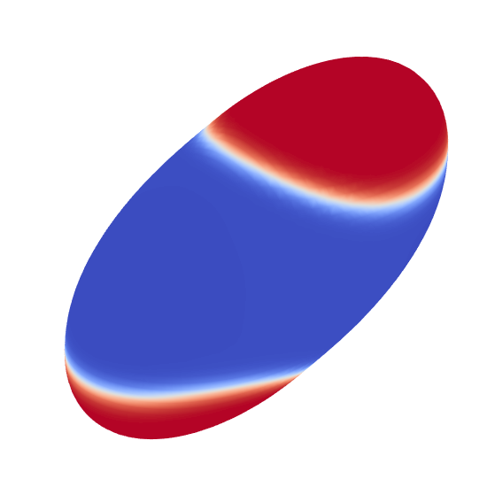
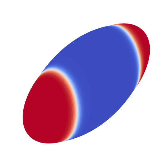
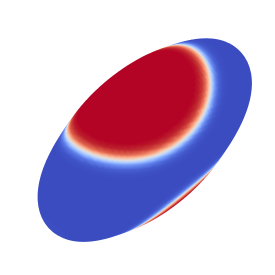
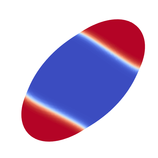
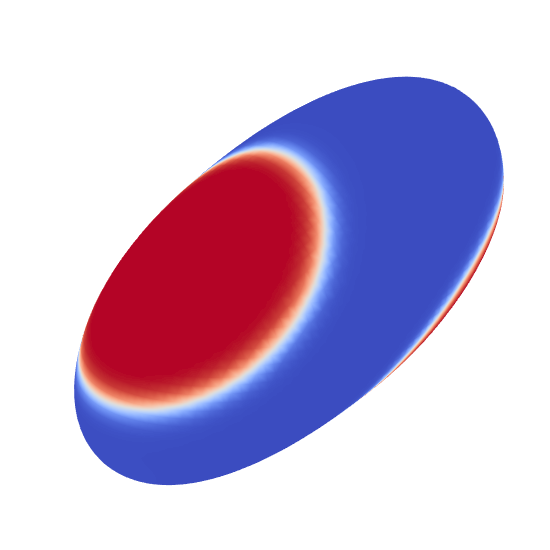
[15pt]$t=2.0$  [15pt]$t=4.0$  [15pt]$t=6.0$  [15pt]$t=10.0$  [15pt]$t=12.5$  [15pt]$t=17.5$  [15pt]$t=20.0$  [15pt]$t=25.0$

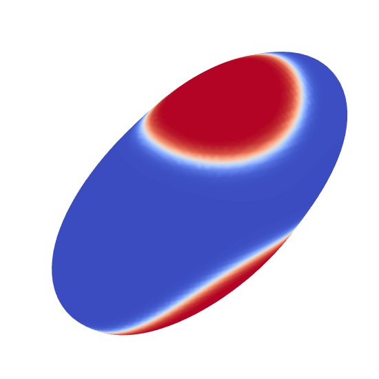
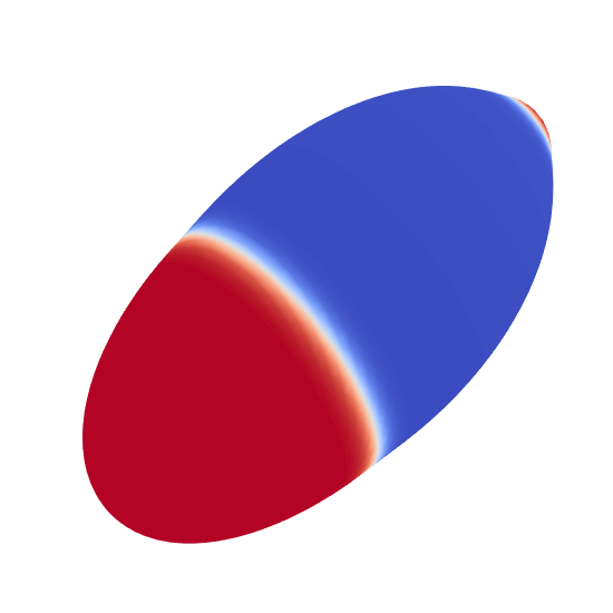
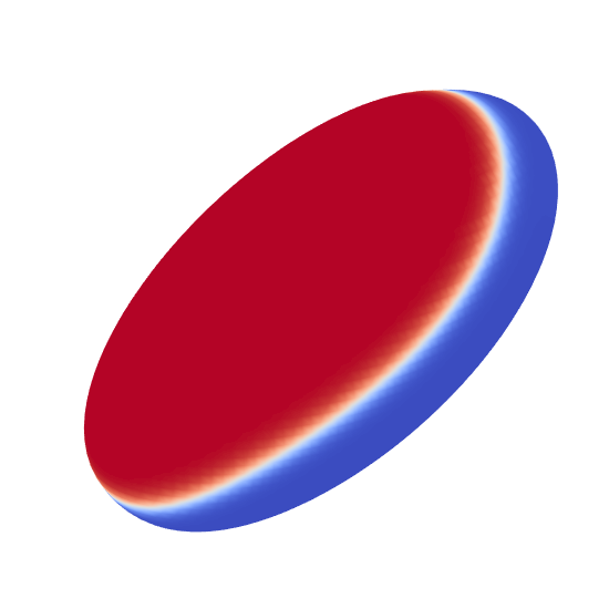
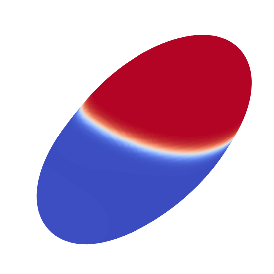
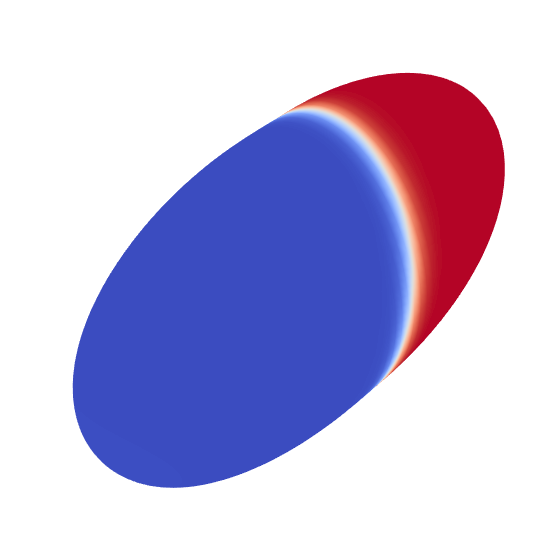
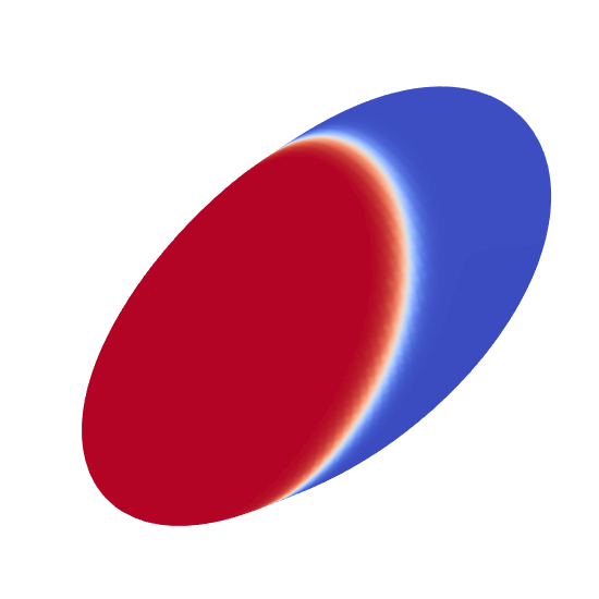
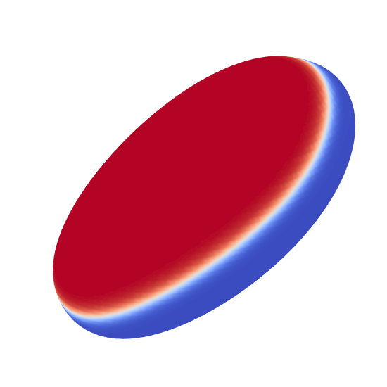
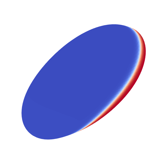
[15pt]$t=27.5$  [15pt]$t=30.0$  [15pt]$t=35.0$  [15pt]$t=37.5$  [15pt]$t=40.0$  [15pt]$t=50.0$  [15pt]$t=52.5$  [15pt]$t=60.0$

Figure 11: Tread-2 dynamics of vesicle with $\bar{c}=0.4$ and $\alpha=0.5$. The soft phase has a bending rigidity of $\kappa_{c}^{B}=0.4$ while the Peclet number is $\textnormal{Pe}=0.3$. These figures are centered on the vesicle.

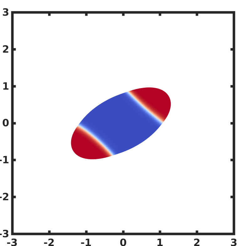
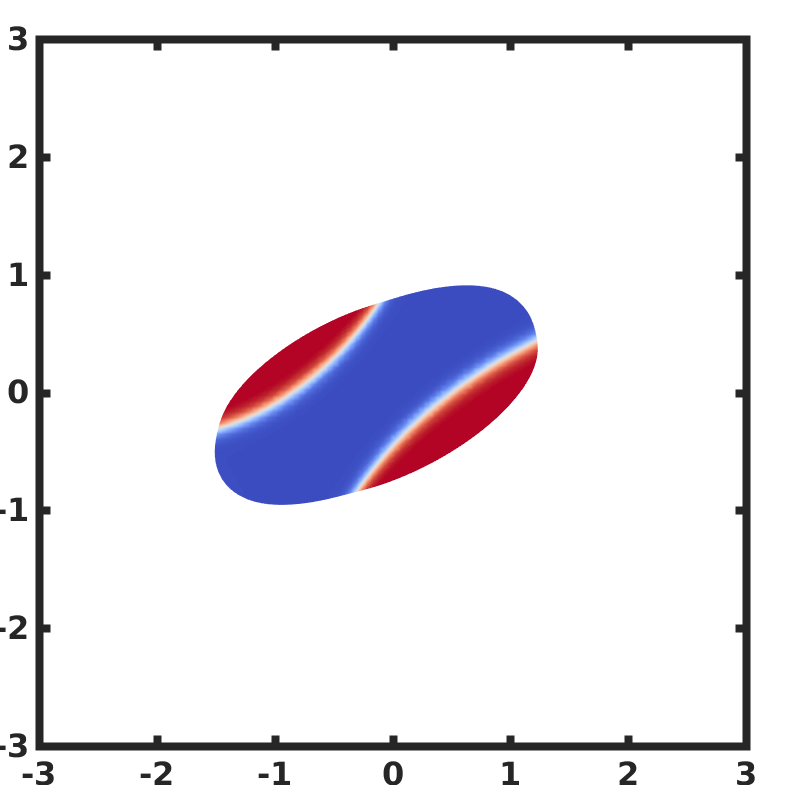
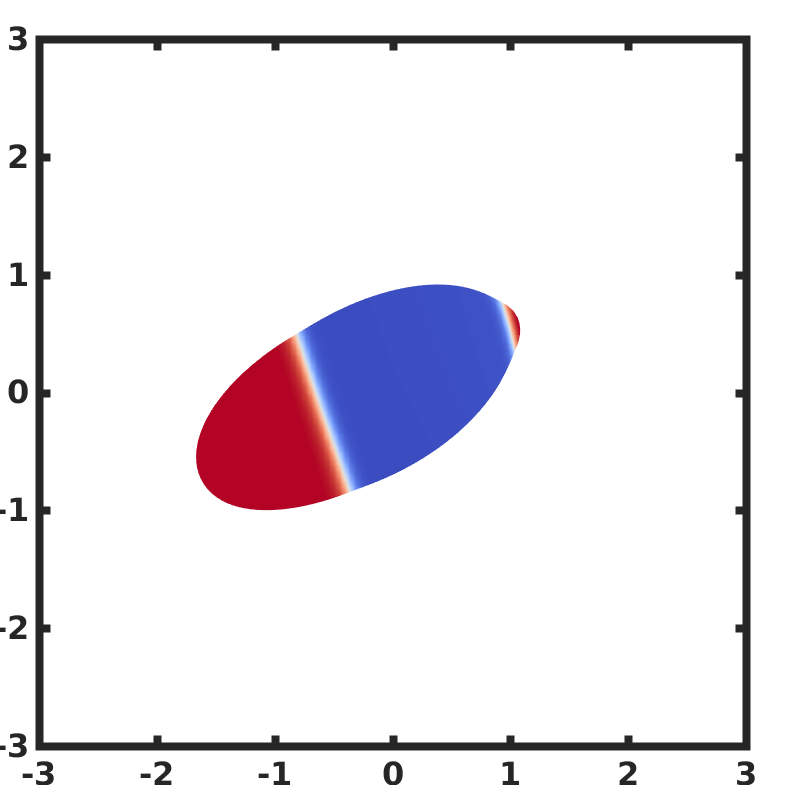
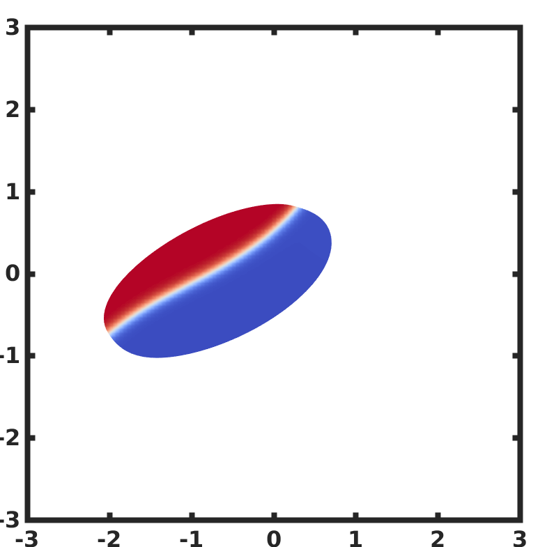
[2pt]$t=20.0$  [2pt]$t=25.0$  [2pt]$t=30.0$  [2pt]$t=35.0$  [2pt]$t=40.0$

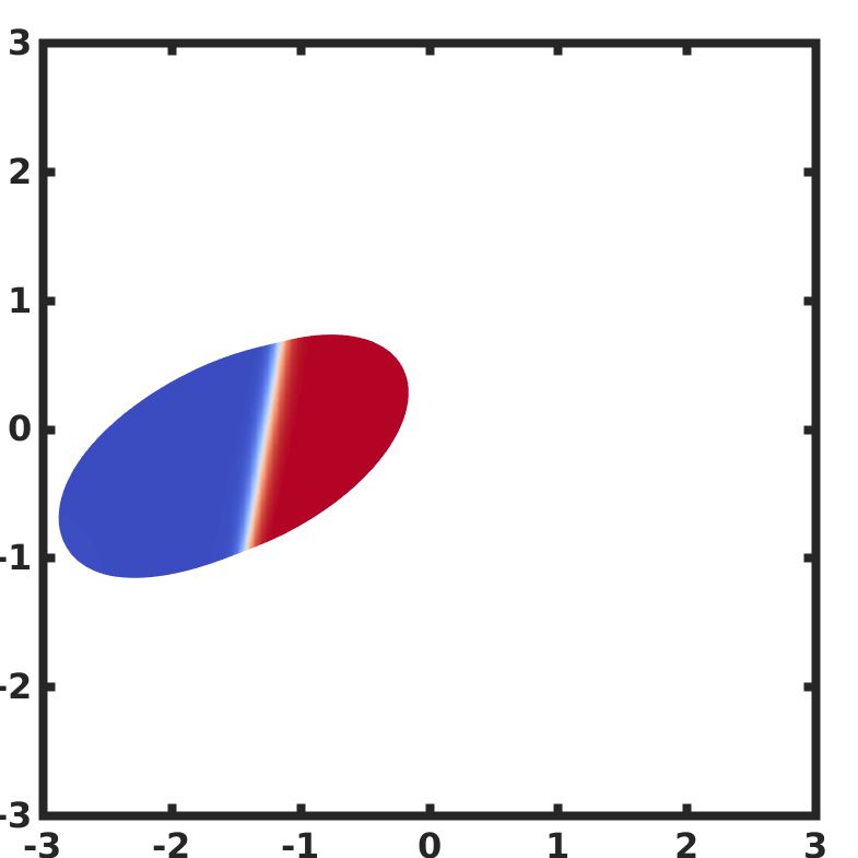
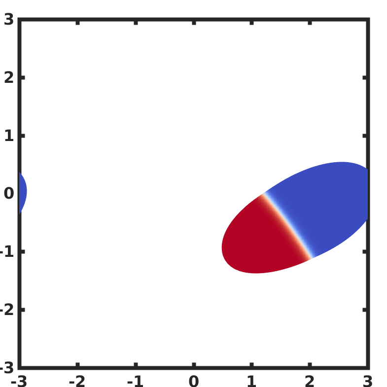
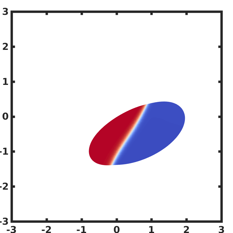
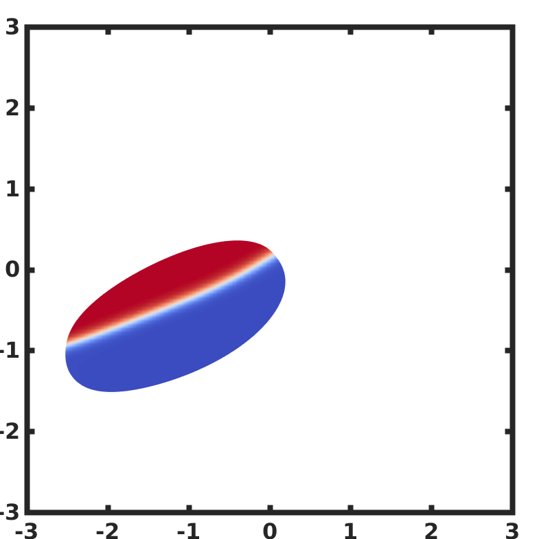
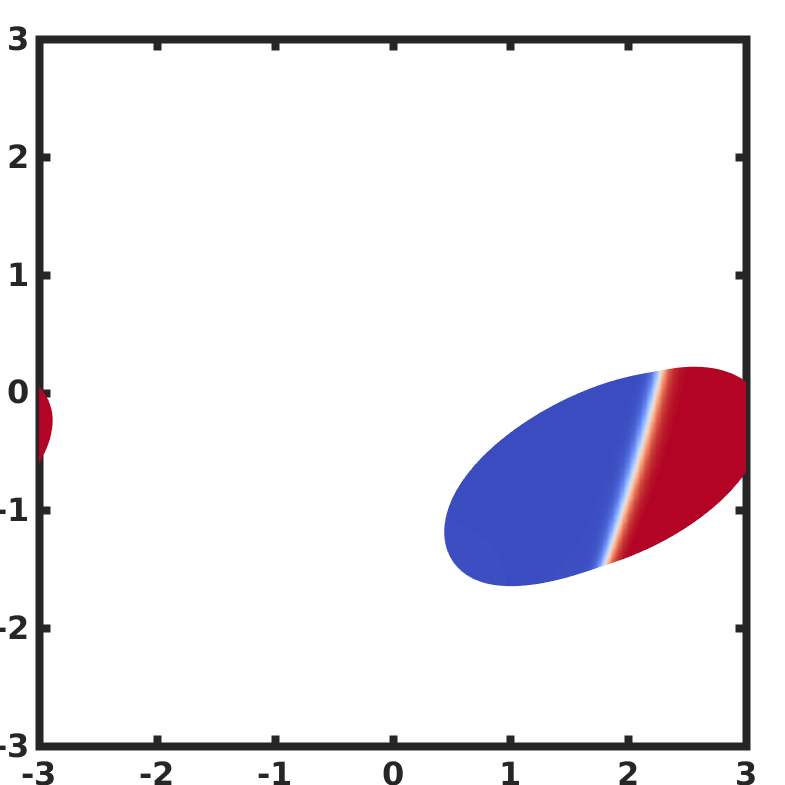
[2pt]$t=47.5$  [2pt]$t=50.0$  [2pt]$t=53.0$  [2pt]$t=57.5$  [2pt]$t=60.0$

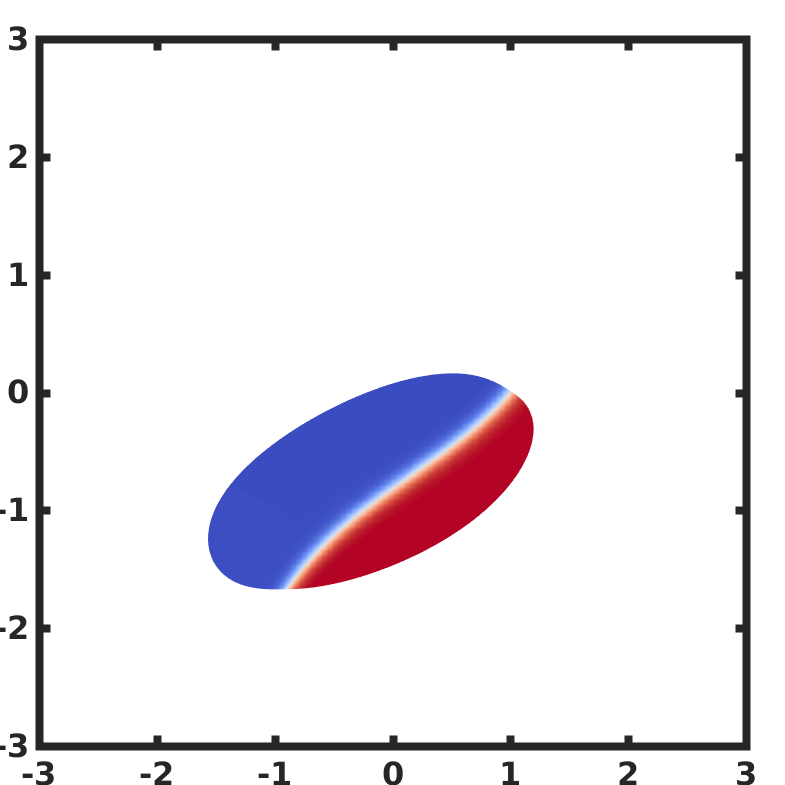
Figure 12: The X-Y plane of the Tread-2 dynamics seen in Fig. 11. The parameters are $\bar{c}=0.4$, $\alpha=0.5$, $\kappa_{c}^{B}=0.4$, and $\textnormal{Pe}=0.3$. A breaking of the symmetry by dissimilar bending rigidities induces motion.

Up to a time of $t=30$, there are two domains phase treading on the membrane with a period of 9.23. At $t=30$, a large drop in the domain boundary energy occurs, which indicates that there is now a single domain on the membrane. After merging, the single domain continues to phase tread, with a lower period of 8.54. See Fig. 13 for the bending and domain boundary energy over time. After merging, the vesicle moves slightly downwards, exposing it to a higher fluid velocity. It is suspected that this is the cause for the decrease in the treading period.

Due to the phase treading of the surface phases, there are periodic fluctuations of the inclination angle. Additionally, after merging the symmetry of the membrane domains is lost, which results in a non-symmetric velocity field. This results in the movement of the vesicle center. See Fig. 14 for the vesicle inclination angle and center over time.

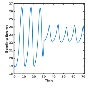
(a) Bending Energy

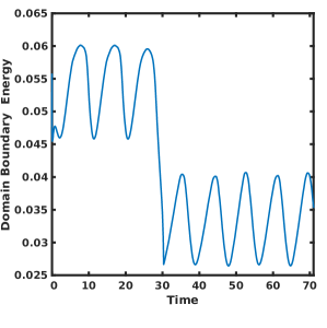
(b) Domain Boundary Energy

Figure 13: The bending and domain boundary energy for the results shown in Fig. 11 and 12. The parameters are $\bar{c}=0.4$, $\alpha=0.5$, $\kappa_{c}^{B}=0.4$, and $\textnormal{Pe}=0.3$.

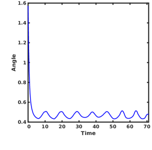
(a) Inclination Angle

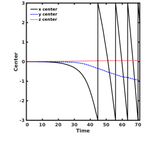
(b) Vesicle Center

Figure 14: The vesicle inclination angle and center location for the results shown in Fig. 11 and 12. The parameters are $\bar{c}=0.4$, $\alpha=0.5$, $\kappa_{c}^{B}=0.4$, and $\textnormal{Pe}=0.3$.

IV Discussion

It is clear from the prior results that the properties of the membrane components play a crucial role in determining the dynamics of the system. To further explore this, consider the amount of time needed for merging, the phase treading period before and after merging, in addition to the phase treading period both before and after merging for a vesicle with $\alpha=0.5$, Fig. 15. The phase treading period is defined as the time between peaks of the bending energy, while the time to merge is calculated as when a large drop in the domain boundary energy occurs and is verified by visually observing the domains on the membrane. Note that the $\alpha=20$ case has too much variation in the domain shapes to provide useful information.

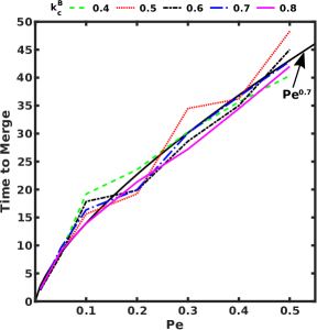
(a) Time to Merge

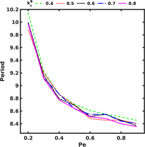
(b) Phase Period Before Merging

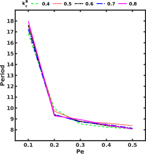
(c) Phase Period After Merging

Figure 15: The time to merge and the phase period as a function of Peclet number for a vesicle with $\bar{c}=0.4$ and $\alpha=0.5$.

As can be seen, the amount of time required for the merging of the two domains into the single domain depends strongly on the surface Peclet number, with the bending rigidity difference between the two phases playing a little-to-no role. Assuming that the limit of the time to merge is zero as Pe approaches zero, the time to merge scales as $\textnormal{Pe}^{0.7}$ for $\alpha=0.5$ and this particular initial condition.

The phase treading period, both before and after merging, depends much more on the surface Peclet number than the bending rigidity difference. Note that the phase periods after merging for Pe values larger than 0.5 are not reported due to the time required to obtain results. Additionally, systems with $\textnormal{Pe}=0.1$ do not under go phase treading before merging, and thus only the period after merging is reported.

In both situations, the phase period appears to decay exponentially with the Peclet number. Following from the prior results, small values of the surface Peclet number result in long phase treading periods, as the soft domains remain at the high curvature tips longer. It is interesting to note that after merging, the phase treading period decreases slightly for all values of Pe.

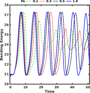
(a) $\kappa_{c}^{B}=0.5$: Bending Energy

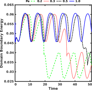
(b) $\kappa_{c}^{B}=0.5$: Domain Boundary Energy

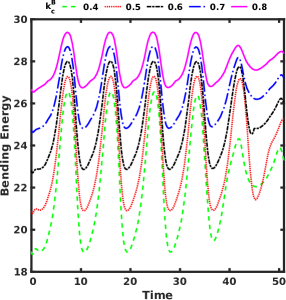
(c) $\textnormal{Pe}=0.5$: Bending Energy

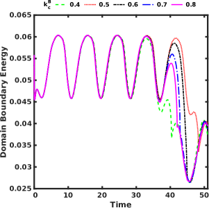
(d) $\textnormal{Pe}=0.5$: Domain Boundary Energy

Figure 16: The bending and domain boundary energies for varying Peclet and bending rigidity for a vesicle with $\bar{c}=0.4$ and $\alpha=0.5$.

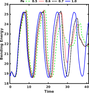
(a) $\kappa_{c}^{B}=0.4$: Bending Energy

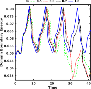
(b) $\kappa_{c}^{B}=0.4$: Domain Boundary Energy

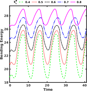
(c) $\textnormal{Pe}=1$: Bending Energy

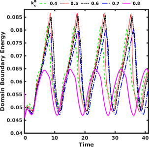
(d) $\textnormal{Pe}=1$: Domain Boundary Energy

Figure 17: The bending and domain boundary energies for varying Peclet and bending rigidity for a vesicle with $\bar{c}=0.4$ and $\alpha=20$.

Finally, consider the bending and domain boundary energy as a function of time for various Peclet numbers and bending rigidities. The results for $\alpha=0.5$ are shown in Fig. 16 while those for $\alpha=20$ are shown in Fig. 17. From these results, several items become apparent. First, the difference between the highest and lowest bending energy during phase treading, denoted as the bending energy gap, depends only on the difference between the bending rigidity of the two phases and not the surface Peclet number. This should be expected, as the bending energy primarily depends on the bending rigidity difference. The surface Peclet number influences the phase treading period, as demonstrated earlier. Additionally, the bending energy and bending energy gap is larger for systems with $\alpha=0.5$ than for systems with $\alpha=20$, see Fig. 18. This is due to the fact that the surface domains deform more for $\alpha=20$ than for $\alpha=0.5$, as shown in prior sections. This allows for more of the phase with the lower bending rigidity to stay in contact with the high curvature tips during phase treading, lowering the overall bending energy.

The shape of the energy curves also follows the prior qualitative results. In particular, for $\alpha=0.5$ the domains remain relatively circular, and thus the domain boundary energy has a relatively smooth transition from high energy values to low energy ones, Fig. 16. For $\alpha=20$, the domains become elongated, with a tail remaining at the vesicle tips. When the domains become too large, the domain tails move very quickly, which is seen as a periodic sharp drop in the domain boundary energy. This behavior is confirmed by comparing the domain boundary energy for $\kappa_{c}^{B}=0.8$ and those for $\kappa_{c}^{B}<0.8$. As the bending energy gap is smaller for $\kappa_{c}^{B}=0.8$ than for the other values, only a small tail is formed, see Fig. 4. Thus, the system with $\kappa_{c}^{B}=0.8$ and $\alpha=20$ behaves more like the $\alpha=0.5$ cases.

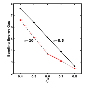
Figure 18: The difference between the maximum and minimum bending energy before domain merging for a vesicle with $\bar{c}=0.4$ with $\alpha=0.5$ or $\alpha=20$. The bending energy gap is not sensitive to variations of Peclet number.

V Conclusions

In this work, the dynamics of a three-dimensional multicomponent vesicle in shear flow has been investigated. The focus of the study was on the influence of the bending rigidity difference, the rate of surface diffusion, and domain boundary line energy on the dynamics. The system in three dimensions allows for inclusion of domain line energy/tension, which results in a more accurate model.

To allow for a systematic study of the influence of properties and parameters, this work focused on initially pre-segregated and symmetric domains. Three types of dynamics were observed: stationary phase, phase treading, and a new dynamic called vertical banding. In general, the dynamics are due to the complex interplay between the difference in domain bending rigidity, the speed of diffusion as measured by the surface Peclet number, and the relative strength of the domain line energy to the bending energy. When the domain line energy is weak, as denoted by a large value of $\alpha$, domains can elongate and form vertical bands. When the line energy is strong, given by small values of $\alpha$, the influence of bending rigidity difference deceases and the dynamics are primarily determined by the surface Peclet number.

Given enough time, all cases considered here will result in a single phase domain. When this occurs the symmetry of the system is lost, and the vesicle begins to tremble about an equilibrium inclination angle. During this time, the vesicle is pulled from the center and begins to migrate laterally.

The results presented here demonstrate that a complete understanding of the dynamics of multicomponent vesicles can only be obtained via fully three-dimensional models. Due to the nature of two-dimensional models, they are not able to capture the full influence of the domain line energy, which has been demonstrated plays a critical role in the determination of the dynamics. In the future, it will be necessary to relax some assumptions made in this work. In particular, the use of a variable surface mobility might better match the physical system. The inclusion of varying fluid density and more complex bending rigidity models may also result in additional interesting dynamics.

Conflicts of interest

There are no conflicts to declare.

References

- Simons and Toomre (2000) K. Simons and D. Toomre, Nature Reviews Molecular Cell Biology, 2000, 1, 31–39.
- Sackmann and Smith (2014) E. Sackmann and A.-S. Smith, Soft matter, 2014, 10, 1644–1659.
- Simons and Vaz (2004) K. Simons and W. L. Vaz, Annual Review of Biophysics and Biomolecular Structure, 2004, 33, 269–295.
- Mukherjee and Maxfield (2004) S. Mukherjee and F. R. Maxfield, Annu. Rev. Cell Dev. Biol., 2004, 20, 839–866.
- Lipowsky and Sackmann (1995) Structure and Dynamics of Membranes, Handbook of Biological Physics, ed. R. Lipowsky and E. Sackmann, North Holland, 1995.
- Baumgart et al. (2003) T. Baumgart, S. T. Hess and W. W. Webb, Nature, 2003, 425, 821–824.
- Veatch and Keller (2003) S. L. Veatch and S. L. Keller, Biophysical journal, 2003, 85, 3074–3083.
- Veatch and Keller (2005) S. L. Veatch and S. L. Keller, Biochimica et Biophysica Acta (BBA)-Molecular Cell Research, 2005, 1746, 172–185.
- Baumgart et al. (2005) T. Baumgart, S. Das, W. Webb and J. Jenkins, Biophysical Journal, 2005, 89, 1067–1080.
- McMahon and Gallop (2005) H. T. McMahon and J. L. Gallop, Nature, 2005, 438, 590–596.
- Lu et al. (2016) L. Lu, W. J. Doak, J. W. Schertzer and P. R. Chiarot, Soft Matter, 2016, 12, 7521–7528.
- Deschamps et al. (2009) J. Deschamps, V. Kantsler, E. Segre and V. Steinberg, Proceedings Of The National Academy Of Sciences Of The United States Of America, 2009, 106, 11444–11447.
- Biben and Misbah (2003) T. Biben and C. Misbah, Physical Review E, 2003, 67, 031908.
- Aranda et al. (2008) S. Aranda, K. A. Riske, R. Lipowsky and R. Dimova, Biophysical journal, 2008, 95, L19–L21.
- Staykova et al. (2008) M. Staykova, R. Lipowsky and R. Dimova, Soft Matter, 2008, 4, 2168–2171.
- Vlahovska et al. (2009) P. M. Vlahovska, R. S. Gracia, S. Aranda-Espinoza and R. Dimova, Biophysical journal, 2009, 96, 4789–4803.
- Kolahdouz and Salac (2015) E. M. Kolahdouz and D. Salac, SIAM Journal on Scientific Computing, 2015, 37, B473–B494.
- Salac and Miksis (2012) D. Salac and M. J. Miksis, Journal of Fluid Mechanics, 2012, 711, 122.
- Vlahovska and Gracia (2007) P. M. Vlahovska and R. S. Gracia, Physical Review E, 2007, 75, 016313.
- Kantsler et al. (2008) V. Kantsler, E. Segre and V. Steinberg, Physical review letters, 2008, 101, 048101.
- Elliott and Stinner (2013) C. M. Elliott and B. Stinner, Communications in Computational Physics, 2013, 13, 325–360.
- Elliott and Stinner (2010) C. M. Elliott and B. Stinner, Journal of Computational Physics, 2010, 229, 6585–6612.
- Barrett et al. (2017) J. W. Barrett, H. Garcke and R. Nürnberg, ESAIM: Mathematical Modelling and Numerical Analysis, 2017, 51, 2319–2366.
- Allain and Ben Amar (2004) J. M. Allain and M. Ben Amar, Physica A-statistical Mechanics and Its Applications, 2004, 337, 531–545.
- Fournier and Ben Amar (2006) J. . B. Fournier and M. Ben Amar, European Physical Journal E, 2006, 21, 11–17.
- Wang and Du (2008) X. Wang and Q. Du, Journal Of Mathematical Biology, 2008, 56, 347–371.
- Funkhouser et al. (2014) C. M. Funkhouser, F. J. Solis and K. Thornton, Journal Of Chemical Physics, 2014, 140, 144908.
- Liu et al. (2017) K. Liu, G. R. Marple, J. Allard, S. Li, S. Veerapaneni and J. Lowengrub, Soft Matter, 2017, 13, 3521–3531.
- Guillemin and Pollack (2010) V. Guillemin and A. Pollack, Differential Topology, Prentice-Hall, 2010.
- Gera and Salac (2018) P. Gera and D. Salac, Computers & Fluids, 2018.
- Chang et al. (1996) Y. Chang, T. Hou, B. Merriman and S. Osher, Journal of Computational Physics, 1996, 124, 449–464.
- Towers (2008) J. D. Towers, Journal of Computational Physics, 2008, 227, 6591–6597.
- Nave et al. (2010) J.-C. Nave, R. R. Rosales and B. Seibold, Journal of Computational Physics, 2010, 229, 3802–3827.
- Seibold et al. (2012) B. Seibold, R. R. Rosales and J.-C. Nave, Discrete & Continuous Dynamical Systems-Series B, 2012, 17, year.
- Velmurugan et al. (2016) G. Velmurugan, E. M. Kolahdouz and D. Salac, Computer Methods in Applied Mechanics and Engineering, 2016, 310, 233–251.
- Fornberg (1988) B. Fornberg, Mathematics Of Computation, 1988, 51, 699–706.
- Chen and Macdonald (2015) Y. Chen and C. Macdonald, SIAM Journal on Scientific Computing, 2015, 37, A134–A155.
- Kantsler and Steinberg (2006) V. Kantsler and V. Steinberg, Physical Review Letters, 2006, 96, 036001.