A bistable belief dynamics model for radicalization within sectarian conflict

Abstract.

We introduce a two-variable model to describe spatial polarization, radicalization, and conflict. Individuals in the model harbor a continuous belief variable as well as a discrete radicalization level expressing their tolerance to neighbors with different beliefs. A novel feature of our model is that it incorporates a bistable radicalization process to address memory-dependent social behavior. We demonstrate how bistable radicalization may explain contradicting observations regarding whether social segregation exacerbates or alleviates conflicts. We also extend our model by introducing a mechanism to include institutional influence, such as propaganda or education, and examine its effectiveness. In some parameter regimes, institutional influence may suppress the progression of radicalization and allow a population to achieve social conformity over time. In other cases, institutional intervention may exacerbate the spread of radicalization through a population of mixed beliefs. In such instances, our analysis implies that social segregation may be a viable option against sectarian conflict.

1. Introduction

Recent years have seen the resurgence of ethnic, religious and racial tension that have created rifts among communities once at peace. In many cases, friction has escalated towards violent conflict, ethnic cleansing and at times even full-fledged civil wars that have destabilized entire social and political systems [18, 27, 24, 20, 3, 7, 30, 4]. The development of viable intervention strategies to mitigate radicalization and violence requires a thorough understanding of the mechanisms underlying sectarian conflict. Identifying the basic ingredients that lead to the emergence of full scale conflict is hindered by the complex nature of human behavior. Instead of simplistic, universal interpretations and solutions, one is often left with contradictory observations and outcomes.

In particular, there is controversy as to whether social segregation should be employed to manage sectarian conflicts [10, 4]. Some studies suggest that inter-ethnic or inter-communal contacts raise tension and that it is beneficial to keep rival communities separate until tensions dissipate [25, 18, 27, 24, 3, 7, 30]. Others have concluded that ethnically mixed environments encourage inter-ethnic friendship and trust, while segregation leads to prejudice and antagonistic behavior [20, 3, 10, 26, 4]. These contradicting conclusions reveal the context-dependent nature of human social behavior.

One of the goals of this paper is to present a mathematical framework that may help resolve basic observations of belief dynamics, radicalization, and conflict. Social studies have shown that humans often hysteretically switch behaviors, perceiving and reacting to the same information in drastically different ways because of different past experiences and circumstantial contexts. This hysteretic switching behavior also applies to general tolerance towards others and their views. Similar socio-economic environments in some cases have led to peaceful coexistence between communities, in others to conflict. Within the context of radicalization we model this hysteresis using a memory-dependent or “bistable” response to the social environment [22, 21]. To quantify this mode-switching behavior, we draw inspiration from the physical sciences, where bistability is ubiquitous; for example, in ferromagnetism where materials switch their magnetic alignment as an external field is varied [5].

Fig. 1(a) depicts the hysteresis curve of a system in which a bistable state variable $\rho$ ($y$-axis) is driven by an independent regulating variable $\sigma$ ($x$-axis). The curve represents the equilibrium solution to, e.g., a differential equation for $\rho$ in which $\sigma$ is a controlling parameter. The solid parts of the curve indicate stable values of $\rho$, while the dashed segment are unstable solutions. The functional dependence of $\rho$ on $\sigma$ yields a window of values $D<\sigma<E$ in which two stable solutions can arise.

Within the context of belief/radicalization dynamics, $\rho$ may represent the degree of radicalization of a population or an individual that is driven by social tension $\sigma$. An interesting and frequently observed phenomenon is that of a slowly deteriorating political, economic or social situation (increasing $\sigma$) which seems under control but abruptly escalates. The lower solid curve indicates a less radicalized population (low $\rho$) that favors peaceful coexistence with others of different views. Increasing social tension can force $\rho$ to transition from the lower to the upper solid curve at $\sigma\geq E$. The upper curve represents a highly radicalized population that is non-tolerant towards those with different views. The “bifurcation point” $E$ thus marks a sudden escalation of sectarian conflict which can be triggered by random events. Once the situation escalates, it is often very difficult to restore peace, as $\rho$ remains on the upper solid curve even if $\sigma$ is decreased back below $E$. Peace can only be restored if sufficient effort is made to further reduce $\sigma$ below the lower bifurcation point $D<E$. The hysteresis between high and low radicalization levels may help shed light on contradicting reports regarding whether the promotion of ethnic mixing or segregation is the best approach to achieve a state of peaceful coexistence. Just like tension can rapidly escalate, it may also rapidly de-escalate. One example might be the decades-long Northern Ireland conflict. As late as 1993, some scholars were still very pessimistic on a possible peaceful resolution of the Catholic/Protestant conflict, stating that: “the cruel conflict will continue, apparently with no end in sight…” [25, 10]. However the 1994 IRA ceasefire quickly lead to the 1998 signing of the Good Friday Agreement, marking the end of “the Troubles.” To phenomenologically incorporate bistability one can, without loss of generality, adopt a simplified description of the relationship between radicalization and tension, as shown in Fig. 1(b).

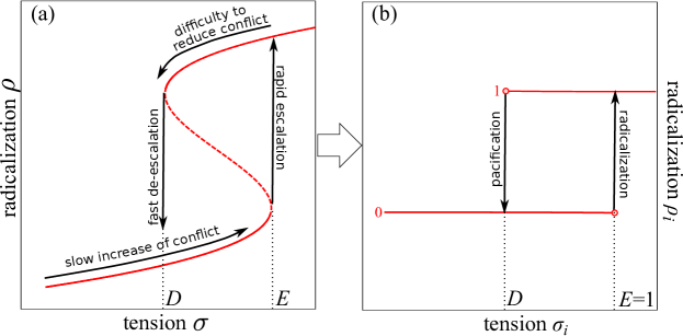
Figure 1. (a) A typical bistability curve. The curve qualitatively captures the essence of escalating conflicts and radicalization $\rho$ due to rising tension $\sigma$. Bifurcation values of the tension $\sigma$ are labelled $D$ and $E$. (b) A simplified piecewise constant description of the bistable dependence of $\rho_{i}$ on $\sigma_{i}$.

To understand influence of behavioral memory on the spread of radicalization and conflict, we will incorporate this bistable dynamics into the belief dynamics model of DeGroot, which describes an individual’s the belief as a one-dimensional continuous variable bounded by two extreme limits [9, 14, 15]. Over time, individuals may change their opinions by interacting with others. In the DeGroot model, originally introduced to study the formation of consensus opinions in a network, conformity is the only ensured outcome. The inability to form heterogeneous distributions of opinions, or “persistent disagreement”, limits the applicability of the model to ethnically or ideologically divergent societies [2, 1, 32, 11]. Extensions of the DeGroot model have been proposed to induce disagreement, such as the popular “bounded confidence” model, where individuals interact only with those holding similar opinions, defined by an opinion range called the bounded confidence [8, 19, 31, 12, 13].

Another approach is taken via “opinion opposition” models that introduce agents of “nonconformity” who adopt contrarian views and cause polarized beliefs and disrupt the formation of consensus [11, 17]. Such models share similarities with spin glass Ising models that describe a mixture of ferromagnetic and antiferromagnetic molecules; the former tend to align their spins with neighbors, while the latter anti-align. Since sectarian conflicts usually arise and progress through direct conflict of opinion, we will adopt an opinion opposition approach rather than a bounded confidence approach. Assuming that opinion differences among individuals causes tension, we incorporate bistability to quantify the level of radicalization that may prompt an individual to radicalize.

We note that relatively peaceful, albeit tense, coexistence between communities of different backgrounds can be ensured by a strong or influential player, such as the state, a dictator, inter-communal institutions, or the international community. The removal of such a player correlates with outbreaks of violent conflicts [10, 16, 30, 6]. Thus, we will also incorporate the influence of a central figure, modeled as a globally connected player exerting institutional influence similar to the concept of media influence on locally connected networks [29].

In the next Section, we present the details of our basic model of radicalization and sectarian conflict. We then augment the basic model to include government propaganda and explore how it influences sectarian conflict. One of our aims is to use our model to inform strategies that can stop radicalization and sectarian violence from spreading among an ethnically mixed population without employing population segregation as a peace-keeping method. Results of our analysis will be presented in the Results and Discussion Section, where parameter dependence will also be explored.

2. Bistable lattice model of conflict

We assume a two-dimensional $N\times N$ site lattice model where each site $i$ is populated by an agent. Two dynamical variables are associated with each agent: a continuous “belief” variable $-1\leq\phi_{i}(t)\leq 1$ indicating the strength of belief in an ideology of agent $i$, and a discrete “radicalization” variable $\rho_{i}(t)\in\{0,1\}$ indicating the intolerance of agent $i$ towards a very different ideology. Since radicalization usually leads to conflict, we will use the two concepts interchangeably. Radicals cause conflict; non-radicals allow for peaceful coexistence. As shown in Fig. 2(a), we color-code the two extreme belief values $\phi=-1$ and $\phi=+1$ blue and red respectively, while lighter colors indicate intermediate values. Despite the continuous belief values, we divide the population into red ($\phi_{i}>0$) and blue ($\phi_{i}<0$) groups and refer them as two sects. We assume a fully occupied periodic lattice without empty sites, and that the occupying agents do not migrate.

The values $\phi_{i}(t)$ and $\rho_{i}(t)$ evolve over time via nearest-neighbor interactions. Nearest neighbors are defined using the “Moore neighborhood,” where eight grid sites surrounding site $i$ are considered, as shown in Fig. 2(b). In the following subsections we describe the model that governs the evolution of $\phi_{i}(t)$ and $\rho_{i}(t)$.

2.1. Belief and radicalization

The magnitude of belief $|\phi_{i}|$ measures the level of enthusiasm of agent $i$. Individuals with $|\phi_{i}|\approx 1$ are belief zealots while those with $|\phi_{i}|\approx 0$ are belief apathetics. In addition to the belief variable $\phi_{i}$, a discrete radicalization variable $\rho_{i}\in\{0,1\}$ describes how an agent perceives other beliefs. An intolerant individual at site $i$ will be assigned $\rho_{i}=1$ and referred to as a radical. Conversely, a tolerant non-radical will be described by $\rho_{i}=0$. Within the context of our model, $\phi$ and $\rho$ describe distinct attributes. Zealots can be tolerant of the opposite sect and be non-radical. For example, zealots may be deeply religious individuals who at the same time are accepting of others’ beliefs.

The site-specific variables $\phi_{i}$ and $\rho_{i}$ depend on each other through an intervening social tension variable $\sigma_{i}$. The basic mechanism for this interplay is that the tension $\sigma_{i}$ felt by agent $i$ arises from differences in belief ($\phi_{i}-\phi_{j}$) between agents $i$ and $j$. In turn, the level of tension $\sigma_{i}$ determines the radicalization state $\rho_{i}$ of agent $i$, who finally adjusts its belief $\phi_{i}$ accordingly. As mentioned in the Introduction, we will assume $\rho_{i}$ to be bistable. The dynamical model is mathematically described below.

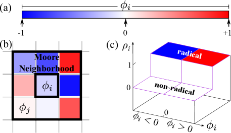
Figure 2. (a) Schematic of the belief variable $-1\leq\phi_{i}\leq 1$. Positive and negative values respectively represent the degrees of belief towards the extreme red and the blue ideologies. The color-coding indicates different values of $\phi_{i}$, with darker colors designated for more zealous beliefs. (b) Definition of nearest neighbors $[i]$. We define nearest neighbors of agent $i$ according to its Moore neighborhood, which include the eight lattice sites surrounding site $i$. (c) Definition and color-code of radicalization $\rho_{i}$. The discrete value of $\rho_{i}$ is determined via the simplified piecewise constant function in Fig. 1(b). $\rho_{i}=1$ represents radicals and is colored red or blue, depending on the corresponding sign of $\phi_{i}$. Non-radicals have $\rho_{i}=0$ and are colored white, regardless of their belief value $\phi_{i}$.

2.2. Tension and belief adaption

The tension $\sigma_{i}$ perceived by agent $i$ is determined as follows:

$$\sigma_{i}[\rho(t),\phi(t)]\equiv\sum_{j\in[i]}J(\rho_{i},\rho_{j})\left(\phi_{i}-\phi_{j}\right)^{2},$$ (2.1)

where the coupling coefficient $J(\rho_{i},\rho_{j})$ characterizes the sensitivity of agent $i$ with radicalization $\rho_{i}$ towards the view expressed by agent $j$ with radicalization $\rho_{j}$. The sum over $j$ is then taken over Moore neighborhood of $i$, $[i]$, as shown in Fig. 2(b).

Eq. 2.1 allows for tensions to increase when neighbors $i$ and $j$ have different belief levels as modulated by $J(\rho_{i},\rho_{j})$. By construction, if all sites neighboring $i$ carry the same belief value $\phi_{i}$, the perceived tension $\sigma_{i}=0$. The functional dependence of $J(\rho_{i},\rho_{j})$ will be defined in the Model Parameters section. Since the maximum of $|\phi_{i}-\phi_{j}|=2$, $0\leq\sigma_{i}\leq 32\,{\rm max}(J)$, where ${\rm max}(J)$ is the maximum of $J(\rho_{i},\rho_{j})$.

The discrete value assigned to $\rho_{i}$ is determined by the piecewise-constant hysteresis function illustrated in Fig. 1(b) and depends on whether $\sigma_{i}$, determined in Eq. 2.1, exceeds a “radicalization point” $E$, is below a “pacification point” $D$, or lies in between. The bistable dependence of $\rho_{i}$ on $\sigma_{i}$ can be expressed as follows

$$\rho_{i}(\sigma_{i}(t))\left\{\begin{array}[]{ll}=1&\textrm{ if }\sigma_{i}(t)>E,\\ =0&\textrm{ if }\sigma_{i}(t)<D,\\ \textrm{unchanged}&\textrm{ otherwise}.\end{array}\right.$$ (2.2)

Since $D$ and $\sigma_{i}$ (and consequently $J$ in Eq. (2.1)) can be rescaled by $E$; without loss of generality, we can set $E\equiv 1$. Phenomenologically, Eq. (2.2) allows high tension to drive a non-radical toward radicalization, while low tension may pacify a radical.

We assume the radicalization state $\rho_{i}$ feeds back to $\phi_{i}$ via a modified continuous-time DeGroot model to include contrarian behavior as follows.

$$\frac{\mbox{d}\phi_{i}(t)}{\mbox{d}t}=\sum_{j\in[i]}k(\rho_{i},\rho_{j},\phi_{i},\phi_{j})\left(\phi_{j}-\phi_{i}\right)$$ (2.3)

where $k(\rho_{i},\rho_{j},\phi_{i},\phi_{j})>0$ is the rate of change of belief from $\phi_{i}$ towards $\phi_{j}$. Negative $k$ indicates a $\phi_{i}$ that drifts away from $\phi_{j}$. The functional dependence of $k$ will be defined in Model Parameters section

Note that Eq. (2.3) can also be written in the form $\phi_{i}(t+\mbox{d}t)=\sum_{j}M_{ij}\phi_{j}(t)$, where $M_{ij}=k(\rho_{i},\rho_{j},\phi_{i},\phi_{j})\mbox{d}t$ for $j\in[i]$, and $M_{ii}\equiv(1-\sum_{j\in[i]}k(\rho_{i},\rho_{j},\phi_{i},\phi_{j}))\mbox{d}t$. For discrete-time DeGroot models $\mbox{d}t=1$ and the matrix $\mathbf{M}$ is known as the “trust matrix” satisfying $\sum_{j}M_{ij}=1$. To prevent $\phi_{i}(t)$ from exceeding the bounds, we further implement no flux boundaries by requiring $k\to 0$ at $\phi_{i}=\pm 1$.

The rules governing the belief value $\phi_{i}$, the intolerance level $\rho_{i}$, and the perceived tension $\sigma_{i}$, are given by Eqs. 2.3, 2.2, and 2.1, respectively. With initial conditions and definitions of the parameter functions $J(\rho_{i},\rho_{j})$ and $k(\rho_{i},\rho_{j},\phi_{i},\phi_{j})$ in the next section, these equations fully define our bistable radicalization and belief dynamics model.

2.3. Model parameters

In this subsection, we define the dependence of $J(\rho_{i},\rho_{j})$ and $k(\rho_{i},\rho_{j},\phi_{i},\phi_{j})$ and then determine the number of independent parameters of the model. We first discuss the coupling function $J(\rho_{i},\rho_{j})$ and assume that interactions with or between radicals heighten the sensitivity towards belief diversity, resulting in higher social tension. We thus assign

$$J(\rho_{i},\rho_{j})=\left\{\begin{array}[]{ll}J_{-}&\textrm{if }\rho_{i}=\rho_{j}=0,\\ J_{+}&\textrm{otherwise},\end{array}\right.$$ (2.4)

where $J_{+}\geq J_{-}\geq 0$ quantify high and low sensitivities.

For the rate of change of belief presented in Eq. (2.3), it is required that $k(\rho_{i},\rho_{j},\phi_{i},\phi_{j})\to 0$ at $|\phi_{i}|=1$ to prevent $\phi_{i}$ from exceeding the bounds. For $|\phi_{i}|<1$, we set $k(\rho_{i},\rho_{j},\phi_{i},\phi_{j})=\pm 1$ to most simply describe conformation and dissension. If agent $i$ finds the belief of its neighbor $j$ agreeable, $\phi_{i}$ “ferromagnetically” adjusts towards $\phi_{j}$ at the rate $k(\rho_{i},\rho_{j},\phi_{i},\phi_{j})=1$. Conversely, if neighbor $j$ antagonizes agent $i$, $k(\rho_{i},\rho_{j},\phi_{i},\phi_{j})=-1$ and $\phi_{i}$ shifts away from $\phi_{j}$, resulting in an “antiferromagnetic” behavior. Finally we assume the following qualitatively reasonable rules to determine whether belief conformation or dissension occurs.

1. A non-radical ($\rho_{i}=0$) conforms to the beliefs of neighboring non-radicals but dissents from the beliefs of radicals ($\rho_{j}=1$), regardless of their belief $\phi_{j}$ of the neighbors. In this case

   $$k(\rho_{i},\rho_{j},\phi_{i},\phi_{j})=\left\{\begin{array}[]{rll}1&\textrm{ if }\rho_{i}=0&\textrm{ and }\rho_{j}=0\\ -1&\textrm{ if }\rho_{i}=0&\textrm{ and }\rho_{j}=1\end{array}\right.$$ (2.5)

2. A radical conforms to the beliefs of neighbors of the same sect and dissents from the beliefs of neighbors of the opposite sect, regardless of their radicalization level. In this case

   $$k(\rho_{i},\rho_{j},\phi_{i},\phi_{j})=\left\{\begin{array}[]{rll}1&\textrm{ if }\rho_{i}=1&\textrm{ and }\phi_{i}\phi_{j}\geq 0\\ -1&\textrm{ if }\rho_{i}=1&\textrm{ and }\phi_{i}\phi_{j}<0\end{array}\right.$$ (2.6)

The above assignment of $k(\rho_{i},\rho_{j},\phi_{i},\phi_{j})$ is summarized in Table 1 below and is illustrated in Fig. 3. The discontinuity of $k(\rho_{i},\rho_{j},\phi_{i},\phi_{j})$ at $|\phi_{i}|=1$ can be made continuous by setting $k(\rho_{i},\rho_{j},\phi_{i},\phi_{j})=\pm\left[1-\tanh((|\phi_{i}|-1)/\epsilon)/2\right]$ with an infinitesimal parameter $\epsilon\ll 1$. For numerical simulations, we may choose $\epsilon$ at the same order as the time step size.

	$\phi_{i}>0$ $\rho_{i}=1$	$\phi_{i}>0$ $\rho_{i}=0$	$\phi_{i}<0$ $\rho_{i}=1$	$\phi_{i}<0$ $\rho_{i}=0$
$\phi_{j}>0$ $\rho_{j}=1$	$+1$	$-1$	$-1$	$-1$
$\phi_{j}>0$ $\rho_{j}=0$	$+1$	$+1$	$-1$	$+1$
$\phi_{j}<0$ $\rho_{j}=1$	$-1$	$-1$	$+1$	$-1$
$\phi_{j}<0$ $\rho_{j}=0$	$-1$	$+1$	$+1$	$+1$

Table 1. The table lists the value of $k(\rho_{i},\rho_{j},\phi_{i},\phi_{j})$, depending on $\rho_{i}$ and $\rho_{j}$, as well as $\phi_{i}$ and $\phi_{j}$.

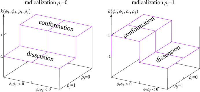
Figure 3. An illustration of the functional dependence of the belief evolution rate $k(\rho_{i},\rho_{j},\phi_{i},\phi_{j})$. Depending on $\rho_{i}$, radicals and non-radicals adopt conformation ($k=1$) and dissension ($k=-1$) behavior differently. Non-radicals ($\rho_{i}=0$, left panel) determine $k$ based on $\rho_{j}$; radicals ($\rho_{i}=1$, right panel) determine $k$ based on the sign of $\phi_{i}\phi_{j}$, i.e., whether individual $j$ belongs to the same sect.

Note that $k(\rho_{i},\rho_{j},\phi_{i},\phi_{j})$ need not be symmetric with respect to the interchange of $i$ and $j$ since individual $i$’s reaction toward individual $j$ will in general be different from that of $j$’s toward $i$. This is a major difference between human interactions and physical interactions, which are typically symmetric.

With the definition of $J(\rho_{i},\rho_{j})=J_{\pm}$ and $k(\rho_{i},\rho_{j},\phi_{i},\phi_{j})=\pm 1$, our equations now have three independent constant parameters: $D$, $J_{+}$ and $J_{-}$. Other adjustable parameters not in the equations include the size $N$ of the periodic lattice and the initial conditions. We vary the initial red-to-blue population ratio, which we denote as $R(0)$, and unless specified otherwise, we set $J_{-}=0.03$, $J_{+}=0.6$, $D=0.1$, $R(0)=3/7$ and $N=100$ as our default parameter values for simulations of Eqs. (2.1)-(2.3). These values are chosen based on our extensive parameter sweep as described in Results and Discussion section.

2.4. Institutional influence

While the basic model (Eqs. (2.1)-(2.3)) describes the spread of radicalization, we may also wish to include intervention strategies that may alleviate conflict. Historically, a more peaceful coexistence of divided populations are facilitated by the presence of a strong or influential central figure, such as a state, a dictator, inter-communal institutions, or the international community [10, 16, 30, 6]. While such a central figure can influence various facets of a society, in this paper we mainly consider how the outreach of government institutions affects social tension.

Figure 4. A global institutional influence function $G(\phi_{i};\phi_{0})$. The function is defined by three parameters: the institutional stance of belief $\phi_{0}$, the strength of the influence $\lambda_{0}$, and the broadness of institutional messages $\ell$. For $\phi_{0}-\ell<\phi_{i}<\phi_{0}+\ell$, $G(\phi_{i};\phi_{0})<0$ and the tension $\sigma_{i}$ decreases. However, outside this range, $\sigma_{i}$ increases.

We model a governmental institution as a globally connected player that adopts a stance $\phi_{0}$ on the belief scale [29]. Institutional publicity or incentives may appease individuals holding similar beliefs to $\phi_{0}$, causing a reduction of the social tension they perceive. However, for individuals with significantly different beliefs compared to $\phi_{0}$, the perceived tension may increase. We model the influence of the institutions on the social tension perceived by agent $i$ via a simple three-parameter quadratic function

$$G(\phi_{i})= \frac{\lambda_{0}}{\ell^{2}}\left(\phi_{i}-\phi_{0}\right)^{2}-\lambda_{0},$$ (2.7)

as plotted in Fig. 4. Under governmental influence, the social tension obeys

$$\sigma_{i}[\rho(t);\phi(t)]= \displaystyle\sum_{j\in[i]}J(\rho_{i},\rho_{j})\left(\phi_{i}-\phi_{j}\right)^{2}+G(\phi_{i};\phi_{0}).$$ (2.8)

The constant $\lambda_{0}$ represents the strength of the institutional influence and is proportional to, say, the available resources and invested efforts. The half distance $\ell$ between the two $x$-axis intercepts characterises the broadness of the institutional message. Within the range $\phi_{0}-\ell<\phi_{i}<\phi_{0}+\ell$, $G(\phi_{i})<0$. Here the institutional message is assumed to be appeasing to individual $i$, leading to the reduction of its social tension $\sigma_{i}$. However, individuals with beliefs outside of this range will experience an increased tension.

For simplicity, we assume that the institutional stance $\phi_{0}$ does not directly sway a belief $\phi_{i}$, leaving Eqs. (2.2) and (2.3) intact. However, an institution may indirectly steer the beliefs of a general population towards its stance by reducing social tensions and thus encouraging conformity towards $\phi_{0}$.

In the following section, we first identify the scenarios that lead to the spread of radicalization in the basic model Eqs. (2.1)-(2.3) without institutional influence. We then include such institutional influence by replacing Eq. (2.1) with Eq. (2.8) and explore the outcomes.

3. Results and discussion

We first examine the basic model Eqs. (2.1)-(2.3) without institutional influence to investigate the dependence of $\phi_{i}$ and $\rho_{i}$ on the five adjustable parameters: $J_{+}$, $J_{-}$, $D$, $N$, and $R(0)$. Simulations of the basic model are carried out by numerically integrating Eqs. (2.1)-(2.3) using a semi-implicit method to update the levels of belief $\phi_{i}$ and radicalization $\rho_{i}$. The numerical discretization is detailed in the Appendix.

The initial conditions of the simulation were set at $\rho_{i}=0$ and randomly drawing values of $\phi_{i}$ from a uniform distribution. We further rebalanced $\phi_{i}$ such that the $\phi_{i}>0$ to $\phi_{i}<0$ (red-to-blue) ratio was $R(0)=3/7$. Next, we placed a radical agent ($\rho^{*}=1$) with belief $\phi^{*}=0.9$ at the center of the lattice. For the rest of the paper, $\rho^{*}=1$ and $\phi^{*}=0.9$ will be used as the initial values of the radical agent at the center of the lattice if such a seed is planted. The results are qualitatively similar for sufficiently extreme values of $\phi^{*}$ ($\phi^{*}\gtrsim 0.9$ or $\phi^{*}\lesssim-0.9$). Uncertainty however rises with smaller $|\phi^{*}|$ as the radical seed tends to be increasingly pacified at the onset of our simulations. A snapshot of $\phi_{i}$ and $\rho_{i}$ at $t=1$ is shown in Figs. 5(a) and (b), respectively, and the default parameter values are used for the simulation. Note that by normalizing $|k(\rho_{i},\rho_{j},\phi_{i},\phi_{j})|$ our simulation time $t$ is defined on the belief-changing time scale.

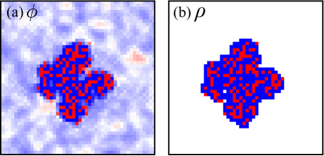
Figure 5. A snapshot of the spatial distribution of (a) $\phi_{i}$ and (b) $\rho_{i}$ during a simulation. (a) The color codes (see Fig. 2(a)) reflect the intensity level of belief, with red and blue indicating the two opposing opinions. (b) The corresponding radicalization values $\rho_{i}$ using the color codes in see Fig. 2(c). The simulation is initiated with $\rho_{i}=0$ and randomly drawn $\phi_{i}$ from a uniform distribution such that $R(0)=3/7$. A radicalized agent with $\rho^{*}=1$ and $\phi^{*}=0.9$ is seeded at the center of the lattice, which triggers the spread of radicalized population. The simulation is conducted on a $100\times 100$ lattice, but the images here are cropped to better show the radicalized population at the center. The other parameters are set to the default values.

In Fig. 5(a) we use the color codes in Fig. 2(a) to depict $\phi_{i}$ for each individual $i$, with darker red/blue colors representing more extreme views among the respective sects. In Fig. 5(b) we plot the corresponding $\rho_{i}$ using the color codes in Fig. 2(c), where radicals are marked by red/blue grids and non-radicals white. As can be seen, radicals tend to exhibit a more extreme level of belief than non-radicals. The latter mostly conform toward relatively neutral beliefs if not in contact with radicals. However, one can still see darker spots in Fig. 5(a) in the regions corresponding to non-radical sites in Fig. 5(b). This shows that regions in which zealots are not radicalized can be sustained, and peaceful coexistence can be achieved. During the simulation, non-radicals can be radicalized by their radical neighbors, leading to an outward spread of radicalization from the initially planted radical seed. Considering that radicalization often precedes conflicts, this “contagion” effect may be referred to as “escalation diffusion” of conflicts, which was identified as a dominant mechanism driving the spread of conflicts [28].

This scenario can also be described as “heterogeneous nucleation” of an “antiferromagnetic” phase within the context of solid state physics. In addition to nucleation by radical agents, under different parameter regimes, our model can also exhibit other qualitatively different dynamics, as displayed in Fig. 6. The behaviors outlined here qualitatively represent those of all possible parameter choices, as confirmed by extensive simulations.

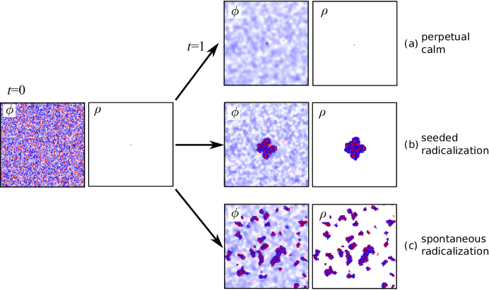
Figure 6. Three typical evolutions of the model Eqs. (2.1)-(2.3): (a) a perpetual calm situation ($J_{-}=0.01$, $J_{+}=0.1$), (b) seeded radicalization ($J_{-}=0.03$, $J_{+}=0.6$), and (c) spontaneous radicalization ($J_{-}=0.06$, $J_{+}=0.4$). The left panel shows the initial conditions of $\phi$ and $\rho$ with an radical seed at the center of the lattice. In the perpetual calm situation, the radical seed is unable to radicalize anyone else. In the scenario of seeded radicalization, radical population spreads out from the initially seeded radical through nearest-neighbor interactions. For spontaneous radicalization, non-radicals turn radical without getting in contact with another radical agent. The other parameters of these simulations $D=0.1$, $R_{0}=3/7$, and $N=100$.

Using the same initial conditions as in Fig. 5 but choosing $J_{-}=0.01,J_{+}=0.1$, Fig. 6(a) depicts a permanently calm situation where $\phi_{i}$ converges towards an intermediate consensus value throughout the lattice except near the initially planted radical. Although its neighboring agents become zealots, as shown by the darker blue colors, they remain non-radical and prevent radical attitudes from spreading. We refer to this outcome as one of “perpetual calm.” Fig. 6(b) displays the same results as in Fig. 5 for $J_{-}=0.03$ and $J_{+}=0.6$. We denote this behavior as “seeded radicalization.” Finally, in Fig. 6(c), the parameters $J_{-}=0.06,J_{+}=0.4$ lead to a hypersensitive system where non-radicals can spontaneously radicalize. Clusters of high tension “antiferromagnetic” domains spontaneously arise in a manner similar to homogeneous nucleation. We call this type of response “spontaneous radicalization.” These three scenarios comprise all qualitatively distinct outcomes of the model seeded with a radical agent at the center of the lattice.

To quantitatively compare the three qualitatively different outcomes shown in Fig. 6, we compute

$$\begin{array}[]{ll}\mbox{(a) mean radicalization:}&\displaystyle\bar{\rho}(t)={1\over N^{2}}\sum_{i}\rho_{i}(t)\vspace{1mm}\\ \mbox{(b) ${(\phi>0)\over(\phi<0)}$ (red:blue) ratio:}&\displaystyle R(t)={\sum_{i}H(\phi_{i})\over\sum_{j}H(-\phi_{j})\vspace{1mm}}\\ \mbox{(c) mean belief value:}&\displaystyle\bar{\phi}(t)={1\over N^{2}}\sum_{i}\phi_{i}(t)\vspace{1mm}\\ \mbox{(d) polarity of belief:}&\displaystyle P(t)={1\over N}\sqrt{\sum_{i}(\phi_{i}(t)-\bar{\phi}(t))^{2}},\end{array}$$ (3.1)

where $H(x)=1$ for $x>0$ and $0$ otherwise is the Heaviside function. Here, $\bar{\phi}(t)$ can be interpreted as a consensus belief, and $P(t)$ is the standard deviation of belief.

Figure 7. Time series of (a) radical fraction $\bar{\rho}(t)$, (b) red-to-blue population ratio $R(t)$, (c) mean belief value $\bar{\phi}(t)$, and (d) polarity of belief $P(t)$ for the scenarios of perpetual calm (solid curves), seeded radicalization (dashed curves), and spontaneous radicalization (dotted curves). For the perpetual calm situation, decreasing $P$ indicates that individual $\phi_{i}$ conforms to a consensus. During the conformation of $\phi_{i}$, red population is converted to blue, as demonstrated by the decreasing $R(t)$. In the other two scenarios, the emergence of radicals eventually causes $\phi_{i}$ to deviate from the consensus, leading to high $P$. The emerging radicals, mainly blue, also prompt non-radical blue individuals to switch sides, leading to a rising trend of $R(t)$. The parameters for each of the three scenarios are the same as in Fig. 6.

Fig. 7(a) shows the radical fraction $\bar{\rho}(t)$ as a function of time. For the case of perpetual calm (solid curve), none of the non-radical agents are turned radical by the planted radical seed, and $\bar{\rho}(t)=1/N^{2}$ throughout the simulation. If the sensitivity $J_{\pm}$ to different neighboring beliefs is increased, radicalization can spread radially from the radicalized seed. The thin dashed curve in Fig. 7(a) shows that the area fraction increases quadratically with time, implying that the typical length scale of the “antiferromagnetic” radicalization phase increases linearly in time. If the minimum sensitivity $J_{-}$ is further increased, tension between neighboring non-radicals with different beliefs is not low enough to prevent spontaneous radicalization. In this case, $\bar{\rho}(t)$ (thick curve) rises quickly to its maximum of unity.

Fig. 7(b) plots the evolution of the red-to-blue population ratio $R(t)$. In the case of perpetual calm, belief conformity prompts all agents to join the majority blue sect. In the other two cases, the minority red sect members initially conform to the blue ideology. However, once the number of radicals increase, some blue non-radicals become alienated by blue radicals and are driven towards a more red belief, progressively turning into red radicals.

Fig. 7(c) shows that under calm conditions the average opinion $\bar{\phi}(t)$ remains constant. Under these conditions $k(\phi_{i},\phi_{j},\rho_{i},\rho_{j})$ is symmetric for every $i$-$j$ pair and $\mbox{d}\bar{\phi}/\mbox{d}t=0$. The value of $\bar{\phi}(t)=-0.2$ is thus set by the initial red-to-blue ratio $R(0)=3/7$. For the two radicalization scenarios, the increasing number of radicals that adopt extreme beliefs causes $\bar{\phi}(t)$ to deviate from $\bar{\phi}(t=0)$.

Finally, in Fig. 7(d) the polarity $P(t)$ shows convergence of $\phi_{i}$ towards a consensus belief in the case of perpetual calm. This is typical for canonical DeGroot models, except that the planted radical seed prevents $P(t)$ from vanishing asymptotically. In the case of seeded radicalization (dashed curve), $P(t)$ initially decreases due to fast conformity followed by a slower increase during which radicalization spreads. If radicalization is spontaneous, the initial conformation phase of decreasing $P(t)$ is overcome by a more rapid radicalization rate that leads to larger polarity.

We find that the sensitivity of non-radicals $J_{-}$ is the primary determinant of whether spontaneous radicalization emerges or not. In Fig. 8(a), we plot radical fractions versus $J_{-}$ for several values of $J_{+}$ at a long time after initiation ($t=50$) to identify the parameter regimes where spontaneous radicalization arises. Initial conditions are set at $\sigma_{i}=0$ and a randomly distributed $-1\leq\phi_{i}\leq 1$ with $R(0)=3/7$. No radical agents are planted at $t=0$.

Figure 8. Parameter dependence of the basic model (Eqs. (2.1)-(2.3)). (a) Spontaneous radicalization triggered by increasing $J_{-}$. Long-time ($t=50$) radical fractions of simulations without initial radical seeds are plotted against $J_{-}$ for various $J_{+}$ values. When $J_{-}$ exceeds a threshold, non-radicals spontaneously radicalize. For long enough time and sufficiently large $J_{+}$, the spontaneously emerging radicals spread through the entire population. (b) Spread of seeded radicalization regulated by $J_{+}$. Radical fractions at an intermediate time ($t=10$) are plotted against $J_{+}$ for various $R(0)$ ratios. A larger $J_{+}$ causes radicals to spread faster, reaching a higher radical fraction at an intermediate time. (c) Intermediate-time ($t=10$) radical fraction versus $R(0)$ for $R(0)\leq 1$. More closely matched initial red and blue populations also result in faster spread of radicals. (d) Time for the radicalization cluster to reach $80\%$ of the system area for various lattice domain size $N$. The time increases linearly with $N$, suggesting a linear radial expansion of the cluster over time. If not varied in the figures, the default parameters values are used. An initial radical seed is planted for figures (b)-(d) but not (a). Each data point represents the mean value of ten simulations, and error bars the standard deviations.

In the absence of a radical seed, non-radicals become radicalized exclusively through the tensions arising from belief differences amongst themselves. We find that spontaneous radicalization is triggered for $J_{-}>0.04$ and that this threshold does not depend on $J_{+}$. For low values of $J_{+}\lesssim 0.2$, the spread of radicals can be arrested after the emergence of spontaneously radicalized patches. As a result, radicals do not pervade society even at long times.

Henceforth, we plant a radical seed at the center and set $J_{-}=0.03$ to focus on seeded radicalization, a qualitatively reasonable description of the nucleation and growth of sectarianism. Recalling that $\sigma_{i}\leq 32{\rm max}(J)$, we have $\sigma_{i}\leq 0.96<1$ if $J=J_{-}$ everywhere, eliminating the chance of spontaneous radicalization. As long as $J_{-}<1/32$, spontaneous radicalization cannot arise. In Fig. 8(b), we plot radical fractions $\bar{\rho}(t=10)$ as a function of $J_{+}$ for various initial red-to-blue ratios $R(0)$. Radicals begin to spread from the planted seed when $J_{+}>0.25$ regardless of $R(0)$. For larger $J_{+}$, the radicalization cluster reaches a larger fraction of the lattice indicating a faster spreading rate. A larger initial ratio $R(0)$ also causes the cluster of radicals to spread at a faster rate. This is confirmed in Fig. 8(c) where radical fraction $\bar{\rho}(t=10)$ for $J_{+}=0.6$ increases with $R(0)$, and is maximal for $R(0)\gtrsim 0.75$, where the members of the two sects are about equal.

These findings are consistent with the observation that conflicts mostly arise in regions where ethnic boundaries were not well-defined (i.e., a mixed population) and where the populations of ethnic groups are closely matched [23]. A minority population that is overwhelmed by a much more populous opposing belief more easily assimilates and is less likely to elicit conflict. An example can be found in Indonesia, where analysis of survey data suggested that the spread of radical beliefs was subdued in villages consisting of a notably dominant majority population [3].

In Fig. 8(d) we plot the time $T_{80}$ for the radicalization cluster to cover $80\%$ of the lattice, which for our simulations corresponds roughly to the time it takes for the cluster perimeter to reach the boundaries of the lattice. We find that $T_{80}$ increases linearly with domain size $N$, suggesting that the radius of radicalized cluster area grows linearly with time, and that the corresponding area scales as $t^{2}$, consistent with Fig. 7(a).

Finally, we find that tension $\sigma_{i}$ rarely decreases among a mixed population, precluding de-radicalization. As a consequence, we find that the value of $D$ has essentially no effect on seeded radicalization in our basic model Eqs. (2.1)-(2.3).

3.1. Global institutional influence

So far we have investigated the parameter dependence of the basic model Eqs. (2.1)-(2.3). We now explore how an external institutional influence may affect radicalization. We set the basic model parameters to the default values ($J_{-}=0.03$, $J_{+}=0.6$, $D=0.1$, $R(0)=3/7$, and $N=100$) and focus on the fast seeded radicalization regime, shown in Fig. 6(b) in the absence of any external players. We here add a global institutional influence $G(\phi_{i};\phi_{0})$ by replacing Eq. (2.1) with Eq. (2.8).

In Fig. 9(a) we plot the long-time ($t=50$) radical fraction $\bar{\rho}(t=50)$ and examine the effect of $\lambda_{0}$, which defines the intensity of the tension-reducing influence. We choose $\phi_{0}=0$ and $\ell=1$, so that the external institution adopts a neutral stance and reduces perceived tension for individuals with any belief value $\phi_{i}$. For these parameters, we observe significant and consistent reduction of radical fractions when $\lambda_{0}\gtrsim 1.6$. For $\lambda_{0}\gtrsim 2.5$, the spread of radicals by the seed is largely suppressed. Hence, one of our major findings is that to exert significant influence $\lambda_{0}$, the institutional influence needs to have a high penetration within the overall population.

In Fig. 9(b), the radical fraction $\bar{\rho}(t=50)$ is depicted using a color intensity map and plotted as a function of $\ell$ and $\lambda_{0}$. As expected, the lowest radicalization levels are achieved by large $\lambda_{0}$ and $\ell$, indicating that for a strong influence intensity to pacify conflicts, the institutional publicity must also have broad appeal. Note that in realistic situations the institutional influence intensity and message breadth are often constrained by the resources available to the institution. It may thus become impractical to simultaneously achieve high penetration and broad appeal given limited resources. How to most effectively allocate resources is an interesting optimization problem.

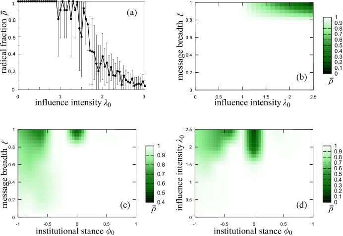
Figure 9. (a) Reduction of radical fraction for various strengths of global institutional influence $\lambda_{0}$. We plot long-time ($t=50$) radical fractions versus $\lambda_{0}$ while setting institutional stance $\phi_{0}=0$ and message breadth $\ell=1$. When $\lambda_{0}\gtrsim 1.6$, the institutional influence begins to show significant effect, and radicals have mostly stopped spreading when $\lambda_{0}\gtrsim 2.5$. (b) Long-time ($t=50$) radical fractions versus $\ell$-$\lambda_{0}$, (c) $\ell$-$\phi_{0}$, and (d) $\lambda_{0}$-$\phi_{0}$. The color maps represent radical fractions. For (b) the institution adopts a neutral stance $\phi_{0}=0$. The most reduction of radicals is achieved at high $\lambda_{0}$ and large $\ell$. For (c), we set $\lambda_{0}=2$. A neutral ($\phi_{0}$) and a majority-biased stance ($\phi_{0}\sim-0.5$) both register significant reduction of radicals. For (d) we choose $\ell=1$, and again $\phi_{0}=0$ and $\phi_{0}\sim 0.5$ results in significant reduction of radicals. Each data point represents the mean value of ten simulations, and error bars in (a) the standard deviations.

In Fig. 9(c) we plot $\bar{\rho}(t=50)$ against $\ell$ and $\phi_{0}$ with $\lambda_{0}=2$. The largest reduction of radicals is occurs in the tongue near the neutral institutional stance $\phi_{0}=0$, but diminishes as $\ell$ is decreased. Some reduction of radicals is also observed when $-1<\phi_{0}<-0.5$, corresponding to a stance biased toward the majority belief. Although this latter regime $-1<\phi_{0}<-0.5$ does not result in as significant a reduction in radical level as the $\phi_{0}\approx 0$ tongue for $\ell\approx 1$, the reduction occurs over a wider range of $\ell$. We thus find that if the institution is unable to fashion a message with sufficiently broad appeal, it may be better bias the influence to appease the majority.

In Fig. 9(d) we show $\bar{\rho}(t=50)$ versus $\lambda_{0}$ and $\phi_{0}$ with $\ell=1$. Again, a neutral institutional stance ($\phi_{0}=0$) achieves the most reduction of radicals, while a majority-biased stance also has some success but to a lesser degree. With respect to influence intensity $\lambda_{0}$, we find that the effectiveness of a majority-biased diminishes quickly with decreasing $\lambda_{0}$, while a neutral stance is capable of maintaining a better result at a lower $\lambda_{0}$.

Our results suggest that an institutional influence achieves optimal results if the entity carefully adopts a strong but neutral stance between the two conflicting beliefs. However, the outreach of the institutional message content is also important. If the institutional influence targets a narrow range of beliefs for the reduction of perceived tension, it may alienate those out of reach, and may have the opposite effect of increasing radicalization. If the institution is unable to placate population with a wide range of beliefs, a stance favoring the majority view may be an effective alternative. Of course, other mechanisms of external influence may apply. For example, governing institutions may directly influence people’s beliefs rather than just the tension they perceive. To model such mechanisms, a modification of Eq. 2.3 can be developed.

4. Conclusions

In this paper, we construct a belief dynamics model that incorporates a bistable radicalization process to describe the spread of sectarian conflict. While the model equations can be applied to arbitrary social network structures, we simulate our model on a locally connected two-dimensional square lattice with periodic boundary conditions. By defining belief and radicalization as separate variables, our model allows for a more nuanced description that distinguishes belief from radicalization. Although in the absence of radicals, all non-radicals asymptotically conform to an apathetic/neutral consensus due to the simplicity of the model, we do observe transient enclaves of more zealous but non-radical individuals. Radicals, on the other hand, are mostly zealots with extreme belief values. We examine the parameter dependence of the model and identify regimes leading to three distinct evolution paths. In the regime of perpetual calm, non-radical individuals cannot be radicalized even if by planting radical seeds in advance. In the regime of spontaneous radicalization, non-radical individuals may spontaneously radicalize even in the absence of radicals. Between the above two regimes lies the regime of seeded radicalization, where non-radical individuals cannot spontaneously radicalize but can become radical upon contact with other radicals. For subsequent investigations, we choose parameter values in the third regime, as the most realistic scenario for the propagation of sectarian conflicts. We find that radicalization can be suppressed by a numerically more dominant majority population between the two competing sects. Finally we implement institutional influence as a globally connected player and find that the most effective intervention to pacify conflict is to adopt a strong but neutral view.

Our model represents a first step in studying the bistable (or multistable) nature of human behaviors in the development of social conflicts. Our incorporation of bistability is only phenomenological, while the underlying mechanism is a fundamental but much more challenging to design and include. Moreover, the separation of ideological belief and radicalization that we propose is a simplified version of multi-dimensional opinion dynamics models. Our modeling framework can be extended to include multiple ideological spectrums, such as religion, social economics, and politics, and examine the interplay among them. Finally, our model can be straightforwardly extended to include evolving, non-lattice social networks.

Appendix: Numerical implementation

For numerical simulations, we adopt a semi-implicit method with a fixed time step size to integrate our model. Let us denote $\phi_{i}(t)$, $\rho_{i}(t)$, and $\sigma_{i}(t)$ at a discrete time $t=n\Delta t$ as $\phi_{i}^{n}$, $\rho_{i}^{n}$, and $\sigma_{i}^{n}$, where $\Delta t$ is the time step size. Then we discretize Eqs. (2.1)-(2.3) as

$$\sigma_{i}^{n+1} = \sum_{j\in{\rm n.n.[i]}}J(\rho_{i}^{n+1},\rho_{j}^{n+1})\left(\phi_{i}^{n+1}-\phi_{j}^{n+1}\right)^{2},$$ (A1)

$$\rho_{i}^{n+1} = \left\{\begin{array}[]{ll}1&\textrm{if }\sigma_{i}^{n+1}>1,\\ 0&\textrm{if }\sigma_{i}^{n+1}<D,\\ \rho_{i}^{n}&\textrm{otherwise},\end{array}\right.$$ (A5)

$$\phi_{i}^{n+1} = \phi_{i}^{n}+\Delta t\sum_{j\in{\rm n.n.[i]}}k(\rho_{i}^{n},\rho_{j}^{n},\phi_{i}^{n},\phi_{j}^{n})\left(\phi_{j}^{n}-\phi_{i}^{n}\right),$$ (A6)

and an iterative method is used to solve the semi-implicit equations (A1)-(A6). The equations with global institutional influence are solved in the same way. Note that for an explicit method, Eq. (2.2) may impose a severe constraint on $\Delta t$, and even with an adaptive time step size, the numerical integration can still be very inefficient.

References

- [1] D. Acemoglu, G. Como, F. Fagnani, and A. Ozdaglar, Opinion fluctuations and disagreement in social networks, Journal of Mathematics of Operations Research 38 (2013), 1–27.
- [2] D. Acemoglu and A. Ozdaglar, Opinion dynamics and learning in social networks, Dynamic Games and Applications 1 (2011), 3–49.
- [3] P. Barron, K. Kaiser, and M. Pradhan, Local conflict in Indonesia: Measuring incidence and identifying patterns, World Bank Policy Research Paper 3384, 2004.
- [4] R. Bhavnani, K. Donnay, D. Miodownik, M. Mor, and D. Helbing, Group segregation and urban violence, American Journal of Political Science 58 (2014), 226–245.
- [5] R. M. Bozorth, Ferromagnetism, IEEE press, New York, 1951.
- [6] A. C. Carpenter, Community resilience to sectarian violence in Baghdad, Springer-Verlag, New York, 2014.
- [7] T. Chapman and P. G. Roeder, Partition as a solution to wars of nationalism: The importance of institutions, American Political Science Review 101 (2007), 677–691.
- [8] G. Deffuant, D. Neau, F. Amblard, and G. Weisbuch, Mixing beliefs among interacting agents, Advances in Complex Systems 3 (2000), 87–98.
- [9] M. H. DeGroot, Reaching a consensus, Journal of the American Statistical Association 69 (1974), 118–121.
- [10] P. Dixon, Why the Good Friday Agreement in Northern Ireland is not consociational, The Political Quarterly 76 (2005), 357–367.
- [11] S. Eger, Opinion dynamics under opposition, http://arxiv.org/abs/1306.3134, 2013.
- [12] K. Felijakowski and R. Kosinski, Bounded confidence model in complex networks, International Journal of Modern Physics C 24 (2013), 1350049.
- [13] by same author, Opinion formation and self-organization in a social network in an intelligent agent system, ACTA Physica Polonica B 45 (2014), 2123–2134.
- [14] N. E. Friedkin, Choice shift and group polarization, American Sociological Review 64 (1999), 856–875.
- [15] B. Golub and M. O. Jackson, Naïve learning in social networks and the wisdom of crowds, American Economic Journal: Microeconomics 2 (2010), 112–149.
- [16] J. Hagan, J. Kaiser, A. R. Hanson, and D. Rothenberg, Neighborhood sectarian displacement and the battle for Baghdad: A self-fulfilling prophecy of crimes against humanity in Iraq, http://ssrn.com/abstract=2118775, 2013.
- [17] M. A. Javarone, Social influences in opinion dynamics: The role of conformity, Physica A 414 (2014), 19–30.
- [18] C. Kaufmann, Possible and impossible solutions to ethnic civil wars, International Security 20 (1996), 136–175.
- [19] U. Krause, A discrete nonlinear and non-autonomous model of consensus formation, Comminications in Difference Equations (S. Elaydi, G. Ladas, J. Popenda, and J. Rakowski, eds.), Amsterdam: Gordon and Breach, 2000, pp. 227–236.
- [20] R. M. Kunovich and R. Hodson, Ethnic diversity, segregation, and inequality: A structural model of ethnic prejudice in Bosnia and Croatia, The Sociological Quarterly 43 (2002), 185–212.
- [21] W. F. Lawless, S. Rifkin, D. Sofge, S. H. Hobbs, F. Angjellari-Dajci, L. Chaudron, and J. Wood, Conservation of information: Reverse engineering dark social systems, Structure and Dynamics 4 (2010), 1–30.
- [22] W. F. Lawless, D. A. Sofge, G. K. Venayagamoorthy, R. Hillson, and C. P. Abubucker, A physics of interdependence for human-robot-machine organizations, IEEE International Conference on System of Systems Engineering, 2009, pp. 1–6.
- [23] M. Lim, R. Metzler, and Y. Bar-Yam, Global pattern formation and ethnic/cultural violence, Science 317 (2007), 1540–1544.
- [24] R. MacGinty, Ethno-national conflict and hate crime, American Behavioral Scientist 45 (2001), 639–653.
- [25] B. O’Leary and J. McGarry, The politics of antagonism, Athlone, London, 1993.
- [26] J. Rydgren, D. Sofi, and M. Hällsten, Interethnic friendship, trust, and tolerance: Findings from two north Iraqi cities, American Journal of Sociology 118 (2013), 1650–1694.
- [27] N. Sambanis, Partition as a solution to ethnic conflict: Some new hypotheses, Security Studies 9 (2000), 1–51.
- [28] S. Schutte and N. B. Weidmann, Diffusion patterns of violence in civil wars, Political Geography 30 (2011), 143–152.
- [29] C. Thron, J. Salerno, A. Kwiat, P. Dexter, and J. Smith, Modeling South African service protests using the national operational environment model, Social Computing, Behavioral-Cultural Modeling and Prediction (S. Yang, A. Greenberg, and M. Endsley, eds.), no. 298-305, Berlin: Springer, 2012.
- [30] N. B. Weidmann and I. Salehyan, Violence and ethnic segragation: A computational model applied to Baghdad, International Studies Quarterly 57 (2013), 52–64.
- [31] G. Weisbuch, G. Deffuant, F. Amblard, and J.-P. Nadal, Meet, discuss, and segregate, Complexity 7 (2002), 55–63.
- [32] E. Yildiz, A. Ozdaglar, D. Acemoglu, A. Saberi, and A. Scaglione, Binary opinion dynamics with stubborn agents, ACM Transations on Economics and Computation 1 (2013), Article 19.