Closed Walk Sampler: An Efficient Method for Estimating Eigenvalues of Large Graphs

Abstract

Eigenvalues of a graph are of high interest in graph analytics for Big Data due to their relevance to many important properties of the graph including network resilience, community detection and the speed of viral propagation. Accurate computation of eigenvalues of extremely large graphs is usually not feasible due to the prohibitive computational and storage costs and also because full access to many social network graphs is often restricted to most researchers. In this paper, we present a series of new sampling algorithms which solve both of the above-mentioned problems and estimate the two largest eigenvalues of a large graph efficiently and with high accuracy. Unlike previous methods which try to extract a subgraph with the most influential nodes, our algorithms sample only a small portion of the large graph via a simple random walk, and arrive at estimates of the two largest eigenvalues by estimating the number of closed walks of a certain length. Our experimental results using real graphs show that our algorithms are substantially faster while also achieving significantly better accuracy on most graphs than the current state-of-the-art algorithms.

1 Introduction

Spectral graph theory, which studies the spectral properties of the Laplacian matrix or the adjacency matrix of a graph, plays an important role in BigData analytics of large graphs [1]. Eigenvalues of a graph (the graph spectrum) can be shown to be related to many principal properties of a graph and have always had applications in chemistry, physics and other applied sciences where graphs are studied and analyzed. In information theory, the channel capacity can be defined in terms of the eigenvalues of the channel graph [2]. In quantum chemistry, the graph spectrum and the corresponding eigenvalues are highly relevant to the stability of the molecule [3]. In Big Data applications involving graphs, such as indexing for web search or social network analysis, eigenvalues of the adjacency matrix can be helpful in characterizing graphs in a variety of ways [4, 5, 6].

In this paper, we focus on the largest and the second largest eigenvalues of the adjacency matrix of the graph. These two eigenvalues have drawn much attention and have been studied extensively for their relationship to multiple graph properties of high relevance. The propagation properties of a graph can be captured by the largest eigenvalue; as presented in [7], an epidemic dies out when the curing rate is larger than the product of the birth rate and the largest eigenvalue. The largest eigenvalue is important to applications related to network robustness, community detection and traffic engineering [8]. Mixing time, the number of steps that a random walk takes to arrive at stationary distribution, is related to the second largest eigenvalue [9]. The spectral gap, the difference between the largest and second largest eigenvalues, can estimate the conductance of the network and describes the connectivity, expansion and randomness properties of the graph [10, 8].

While the study of the largest and the second largest eigenvalues has attracted much research, efficient computation of these eigenvalues in case of massive graphs remains an unsolved problem. The extremely large size of many graphs of interest today (e.g., social network graphs) makes it difficult, or sometimes even infeasible, to compute certain complex properties of these graphs such as its eigenvalues. Power iteration, one of the most famous and widely used algorithms for calculating the largest eigenvalue and its associated eigenvector, requires $O(|E|)$ at each iteration ($|E|$ is the number of edges in the graph)[11]. This method can also be used to calculate the second largest eigenvalue if the eigenvector of the largest eigenvalue is given or is calculated first.

Restricted access to the full graph is the other barrier to researchers being able to compute the eigenvalues of large graphs. The complete structural information of most social network graphs (e.g., Facebook) is hidden except to privileged users with access to the internal servers of the companies hosting the network. Thankfully, however, on most online social networks, the neighboring nodes of a given node can be queried via its API for developers. This feature enables a random walk on the graph and becomes one of the only means by which a large restricted-access graph can be studied for its most interesting properties such as its eigenvalues.

The goal of this paper is to develop new sampling algorithms which overcome the two obstacles mentioned above, the prohibitive computational and storage costs and the matter of restricted access to the entire graph. This work proposes new efficient algorithms which estimate the two largest eigenvalues of a large graph by sampling only a small fraction of the graph by means of a random walk.

1.1 Contributions

A closed walk or a closed path on a graph is a sequence of nodes starting and ending at the same node. Our contribution exploits the fact that the number of closed walks of length $k$ is equal to the $k$-th spectral moment of a graph. Thus, estimating the number of closed walks of length $k$ in a large graph allows us to estimate the top eigenvalues of the graph. Based on this principle, we present a series of new sampling algorithms with increasing generalizations. They carry the name Closed Walk Sampler, abbreviated as cWalker, and can estimate the top eigenvalues of a graph by visiting only a small fraction of the graph via a random walk.

Section 2 presents the theoretical foundation behind the Closed Walk Sampler. We show that the largest eigenvalue of the graph can be inferred from the probability with which a closed path of length $k$ is observed in the random walk. We examine the variance and the confidence interval of our estimate of the number of closed paths in order to illustrate the issue of large deviations in the estimate when observations of a closed path become rare. This section builds the rationale for increasing the probability of observing closed walks in the random walk.

In Section 3, we propose cWalker-A, which accepts a parameter $k$ and uses an estimate of the number of closed walks of length $k$ to return an estimate of the largest eigenvalue of the graph. This version of our algorithm examines all the neighbors of nodes visited during the random walk to see if it can find a closed path without directly traversing a closed path in the random walk, thus increasing the probability of observing closed paths. The cWalker-A algorithm is named cWalker-limited in our preliminary work [12].

Section 4 presents cWalker-B, a generalization of cWalker-A. It is named the cWalker algorithm in our preliminary work [12]. Instead of accepting a parameter $k$ as an input, it computes a reasonable value of $k$ which provides a good balance between the accuracy and the computational cost under the constraints of meeting a certain accuracy target. This section also describes the theoretical basis behind the algorithm.

Section 5 presents a generalized approach to estimate the top $n$ eigenvalues of a graph iteratively. In Section 6, we propose the cWalker-C algorithm, a generalization of cWalker-B based on eigenvalues. It estimates the two largest eigenvalues at the same time.

In Section 7, we present a performance analysis of our algorithms, cWalker-B and cWalker-C, against other state-of-the-art algorithms. Section 8 concludes the paper.

1.2 Related Work

A large amount of work has focused on computing the eigenvalues and their associated eigenvectors of matrices and graphs. The naive method for exactly computing the eigenvalues of a matrix needs to find the roots of the characteristic polynomial of the matrix [1]. However, computing the roots of the characteristic polynomial of even a small matrix can be expensive and time-consuming, which makes it computationally infeasible for the adjacency matrices of large graphs.

One class of approaches has tried to develop algorithms which produce approximations to the eigenvalues and associated eigenvectors[13, 14, 15, 16, 17]. These algorithms are iterative, with better approximations at each new iteration. The Power Iteration is among the most famous and popular iterative algorithms for finding the largest eigenvalue and its associated eigenvector [11]. The iteration is terminated when two consecutively calculated values of the largest eigenvalue are sufficiently close.

Besides the Power Iteration, a number of other iterative algorithms and their variations have been widely studied and have been used in research. Subspace Iteration [18, 19] can produce several of the largest eigenvalues and associated eigenvectors of a symmetric matrix. Inverse Iteration [15, 20] and Rayleigh Quotient Iteration [16] are modifications of the Power Iteration. They require fewer iterations, and obtain a faster convergence than the original Power Iteration. QR algorithm[17] computes all eigenvalues and associated eigenvectors; due to its complexity, it is often applied only to small matrices. An overview of some popular iterative methods for computing eigenvalues and eigenvectors, along with a summary of their advantages and drawbacks, can be found in [21].

All of these iterative methods require the complete information about the graph, while in our case we assume the reality we face in the analysis of large social network graphs — that the access to the full graph is restricted. Unfortunately, therefore, none of the above approaches can serve as a feasible solution to the problem of estimating the eigenvalues of a large graph accessible only through a limited API made available to developers.

A different approach to understanding the eigenvalues of a graph is through examining properties of a graph and inferring mathematical bounds on them [22, 23, 24, 25, 26]. However, these bounds can only serve as a rough guide and are not tight enough to provide an accurate estimate of the top eigenvalues.

A third and more feasible approach to estimating complex properties of large graphs is through sampling. Sampling approaches have been widely used in research on estimating simple but key properties of graphs such as the degree distribution, the global clustering coefficient, centrality metrics, and motif statistics[27, 28, 29]. One approach to graph sampling has been through extracting, via sampling, a small representative subgraph from the large graph [30] and projecting the properties of the subgraph on to the complete graph. While these graph sampling methods have largely focused on simple graph properties, much less is known about sampling a large graph efficiently to estimate more complex properties such as its spectrum or even just its largest eigenvalue.

The body of research that comes closest to our work tries to find the most influential nodes via eigenvalue centrality approximation. They work by collecting these nodes into a subgraph sample and one can then compute the largest eigenvalue of this subgraph to estimate the largest eigenvalue of the full graph based on interlacing results in spectral graph theory which allow one to bound the eigenvalues of the full graph using the eigenvalues of its subgraphs. In [31], the authors present the Expansion Sampling algorithm (XS) which is capable of capturing various centralities (including eigenvalue centrality) of the nodes. In this method, a subgraph sample is maintained where a neighboring node of the subgraph is added into the subgraph based on the number of its neighbors that are neither in the current subgraph nor are the neighboring nodes of the current subgraph sample. Cho et al. propose the BackLink Count (BLC) algorithm which collects nodes that have most neighbors into its sample subgraph [32]. In [33], the authors propose a greedy algorithm called Spectral Radius Estimator (SRE), which samples nodes with the largest neighborhood volume and adds them into its subgraph. The algorithm tries to extract out of the full graph a subgraph with as large a spectral radius as possible.

While these algorithms based on sampling the nodes with the largest eigenvalue centrality in the graph offer some promise, they all need to compute some metric or a score, that is hypothesized to correspond to eigenvalue centrality, for each neighboring node of the current sample subgraph in order to select the node with the highest score. This leads to high computational complexity. The algorithms proposed in this paper avoid the computational and space complexity associated with such calculations and estimate the largest and the second largest eigenvalues via a simple random walk.

2 The Rationale

In this section, we present the theoretical foundation for the Closed Walk Sampler (cWalker). We illustrate the problem of large deviation in the estimates made of the number of closed walks of any given length and explain why we focus on increasing the probability of observing a closed path during the random walk on the graph.

2.1 Preliminaries and Notation

Consider a connected, undirected simple graph $G=(V,E)$ with node set $V$ and edge set $E$. Let $v\in V$ denote a node in $G$ and let $N(v)$ denote the set of neighbors of node $v$. Let $d(v)$ denote the degree of node $v$ and let $D=\sum_{v\in V}d(v)$ denote the sum of the degrees of all the nodes in $G$.

Let $A$ be the $|V|\times|V|$ adjacency matrix of graph $G$. Since $G$ is an undirected graph, $A$ is symmetric and its eigenvalues are all real. Let $\lambda_{1}\geq\lambda_{2}\geq...\geq\lambda_{|V|}$ denote the real eigenvalues of $A$. $\lambda_{1}$ is the largest eigenvalue of its adjacency matrix. The goal of our paper is to estimate the value of $\lambda_{1}$ by visiting only a small portion of the large graph via a random walk.

Consider a random walk on $G$, $(r_{1},r_{2},r_{3},...)$, where $r_{1}$ is the starting node and $r_{i}$ denotes the node visited in step $i$. Let $t$ denote the mixing time of graph $G$. Mixing time is the number of steps that a random walk takes to reach steady state distribution [9]. The mixing time describes how fast a random walk converges to its stationary distribution.

Let $P^{(i)}(v_{j})$ be the probability of visiting node $v_{j}$ in step $i$. The probability of drawing a given node from the stationary distribution is independent of the initial node chosen to begin the random walk. Thus, for $i\geq t$ (random walk reaches the mixing time), we can drop $i$ from the notation and let $P(v_{j})$ denote the probability of visiting node $v_{j}$ in the stationary distribution. As shown in [9],

$$P(v_{j})=\frac{d(v_{j})}{D}$$

Let ${\bf R}^{(k)}$ denote the set of all possible sequences of $k+1$ nodes which can be traversed in a random walk in $G$; it is the set of all walks of length $k$ (allowing repeated nodes) in $G$. Let $X^{(k)}=(x_{1},x_{2},...,x_{k},x_{k+1})$ denote a sequence of $k+1$ nodes such that $X^{(k)}\in{\bf R}^{(k)}$. $X^{(k)}$ is a closed walk if $x_{1}=x_{k+1}$.

Let $P(X^{(k)})$ denote the probability that the random walk steps through exactly the sequence of nodes $X^{(k)}$. Then, $P(X^{(k)})$ is given by

$$P(X^{(k)}) = \frac{d(x_{1})}{D}\frac{1}{d(x_{1})}\frac{1}{d(x_{2})}\cdots\frac{1}{d(x_{k})}$$ (3)

$$= \left\{\begin{array}[]{ll}{\displaystyle\frac{1}{D}\prod_{i=2}^{k}\frac{1}{d(x_{i})}},&\mbox{$k>1$ }\\ {\displaystyle\frac{1}{D}},&\mbox{otherwise.}\end{array}\right.$$

Now, define the function $\omega(X^{(k)})$ as follows to indicate if $X^{(k)}$ is closed:

$$\omega(X^{(k)})=\left\{\begin{array}[]{ll}1&\mbox{if $x_{1}=x_{k+1}$}\\ 0&\mbox{otherwise.}\end{array}\right.$$

Given any sequence of nodes visited in the random walk, the probability of visiting any particular sequence can be calculated using Eqn. (3). The value of function $\omega(X^{(k)})$ for the sequence can be obtained by checking if the first and last nodes in the sequence are the same.

2.2 Relationship to the number of closed walks

An interesting fact about graph spectra is that the trace of the $k$-th order of the adjacency matrix of a graph equals its $k$-th spectral moment [4]:

$$\mathrm{tr}(A^{k})=\sum_{i=1}^{|V|}\lambda_{i}^{k},$$ (4)

where $A$ is the adjacency matrix of the graph and $\mathrm{tr}(A^{k})$ denotes the trace of the matrix $A^{k}$.

The number of closed walks of length $k$ in $G$ is equal to the trace of matrix $A^{k}$ [4]. Therefore, we have

$$\sum_{X^{(k)}\in{\bf R}^{(k)}}\omega(X^{(k)})=\mathrm{tr}(A^{k})$$

Applying Eqn. (4),

$$\sum_{X^{(k)}\in{\bf R}^{(k)}}\omega(X^{(k)})=\sum_{i=1}^{|V|}\lambda_{i}^{k}$$ (5)

For large values of $k$, $\lambda_{1}^{k}$ becomes the dominant term in the RHS of Eqn. (5). Thus, we can get

$$\sum_{X^{(k)}\in{\bf R}^{(k)}}\omega(X^{(k)})\approx\lambda_{1}^{k}$$ (6)

The above equation shows that we can arrive at an approximation of the largest eigenvalue $\lambda_{1}$ if we know the number of closed walks of length $k$ in $G$.

For any walk of length $k$, $X^{(k)}$, using Eqn. (3) we define function $f(X^{(k)})$ as follows,

$$f(X^{(k)})=\frac{1}{P(X^{(k)})D}$$ (7)

Let ${R_{i}}^{(k)}=(r_{i-k},r_{i-k+1},...,r_{i})$ denote a walk of length $k$ obtained in the random walk during steps $i-k$ through $i$, where ${R_{i}}^{(k)}\in{\bf R}^{(k)}$. Taking the expected value of $\omega({R_{i}}^{(k)})f({R_{i}}^{(k)})$, we have

$$\mathrm{E}[\omega({R_{i}}^{(k)})f({R_{i}}^{(k)})]$$

$$~{}~{}=\sum_{X^{(k)}\in{\bf R}^{(k)}}P(X^{(k)})\mathrm{E}[\omega({R_{i}}^{(k)})f({R_{i}}^{(k)})|{R_{i}}^{(k)}=X^{(k)}]$$

$$~{}~{}=\sum_{X^{(k)}\in{\bf R}^{(k)}}P(X^{(k)})\omega(X^{(k)})f(X^{(k)})$$

$$~{}~{}=\frac{1}{D}\sum_{X^{(k)}\in{\bf R}^{(k)}}\omega(X^{(k)})$$ (8)

Using Eqns. (3) and (6), we get

$$\lambda_{1}^{k}\approx\left\{\begin{array}[]{ll}{\displaystyle D\cdot\mathrm{E}\left[\omega({R_{i}}^{(k)})\prod_{j=1}^{k-1}d(r_{i-j})\right]},&\mbox{$k>1$}\\ D\cdot\mathrm{E}[\omega({R_{i}}^{(k)})],&\mbox{$k=1$}\end{array}\right.$$ (9)

According to Eqn. (9), we can come up with a simple algorithm for estimating $\lambda_{1}$ by random walk. At each step, we check if the previous $k+1$ nodes form a closed path. By checking for a closed path during the random walk, we estimate the number of closed walks of length $k$ in $G$. Then, we can easily reach an approximation of $\lambda_{1}$.

2.3 Estimate of $D$

As presented in Eqn. (9), the value of $D$, the sum of the degrees of all the nodes in $G$ is required in order to compute $\lambda_{1}$. Since we assume that the access to the full graph is restricted, the real value of $D$ remains unknown. However, we can generate an estimate of the value of $D$ via random walk.

Consider the expected value of $1/d(r_{i})$ over the random walk, where $r_{i}\in V$ is the node visited in step $i$:

$$E\left[\frac{1}{d(r_{i})}\right] = \sum_{v\in V}\frac{d(v)}{D}\frac{1}{d(v)}=\frac{|V|}{D}$$ (10)

Eqn. (10) suggests a naive way of estimating the value of $D$. D is equal to the ratio of the total number of nodes in the full graph to the expected value of the degree of the nodes visited in the random walk. In this paper, we focus on the estimate of the largest eigenvalue, so we assume that the total number of nodes is already known. In many social networks, e.g., Flickr, the total number of nodes is known.

When the total number of nodes is not actually known, some approaches that estimate it via a random walk have been presented in [34, 35, 36]. These approaches can be easily combined with our method. So, in the case that we do not know the number of nodes in advance, we still can estimate it and proceed with our algorithm.

2.4 Large deviation

Theoretically, according to Eqn. (9), the approximation of $\lambda_{1}$ is closer to the actual value if a larger value of $k$ is applied. How does the selection of $k$ affect the accuracy? Since the approximation of $\lambda_{1}$ is obtained from the estimate of $\sum_{X^{(k)}\in{\bf R}^{(k)}}\omega(X^{(k)})$, here we analyze the performance of estimating the number of closed walks of length $k$ as a reference.

Using Eqn. (2.2), we get the variance of the estimate of

$${\displaystyle\sum_{X^{(k)}\in{\bf R}^{(k)}}\omega(X^{(k)})}$$

as follows:

$$\mathrm{Var}[D\omega({R_{i}}^{(k)})f({R_{i}}^{(k)})]$$

$$=\mathrm{E}[(D\omega({R_{i}}^{(k)})f({R_{i}}^{(k)}))^{2}]-\mathrm{E}[D\omega({R_{i}}^{(k)})f({R_{i}}^{(k)})]^{2}$$

$$=\sum_{X^{(k)}\in{\bf R}^{(k)}}\omega(X^{(k)})\left(\frac{1}{P(X^{(k)})}-1\right)$$ (11)

The above equation shows that the deviation of the estimate becomes larger as a larger value of $k$ is used. Let $\tilde{{\bf R}}^{(k)}$ denote the estimate of the number of closed walks of length $k$ in $G$. A 95% confidence interval for the estimate $\tilde{{\bf R}}^{(k)}$ is as follows:

$$\left(\tilde{{\bf R}}^{(k)}-1.96\frac{\sigma}{\sqrt{n}}~{},~{}~{}\tilde{{\bf R}}^{(k)}+1.96\frac{\sigma}{\sqrt{n}}\right),$$

where $\sigma^{2}$ is the variance of $\tilde{{\bf R}}^{(k)}$, and $n$ is the length of the random walk.

As the above expression shows, the size of the confidence interval is determined by $\sigma$ and $n$. This suggests that, for a larger value of $k$, we have to increase the length of the random walk in order to reach a better accuracy on the estimation of the number of closed walks of length $k$.

Eqn. (11) shows that the probability of visiting a closed walk of length $k$ significantly affects the deviation of the estimate. In many network graphs, the ratio of the number of closed walks of a certain length $k$ to the total number of walks of that length is very low for large $k$. It makes the observation of a closed walk of a large length become a rare event, and thus leads to a large deviation of the estimate. In order to improve the probability with which we observe a closed walk of a given length, we propose the cWalker-A, a basic version of our algorithm which examines paths beyond the ones traversed by the random walk itself.

3 Algorithm given $k$ (cWalker-A)

In this section, we present cWalker-A, which estimates the largest eigenvalue of a graph through a random walk based on estimating the number of closed walks of a given length, $k$. The cWalker-B algorithm presented in the next section generalizes the cWalker-A to find the most appropriate length of closed walks to observe and upon which to base the estimate of the largest eigenvalue.

In the naive method suggested by Eqn. (9), an observation of a closed path in the random walk is confirmed by checking whether the first and the last nodes in the path are the same. It works fine when the value of $k$ is not too large. However, as a larger value of $k$ is applied, the large deviation problem becomes severe. The key to the solution of this problem is to increase the probability of visiting a closed walk of any given length. Based on this intuition, our approach checks if a path is closed by examining the neighboring nodes of the penultimate nodes in the potential path.

Define the function $\phi(X^{(k)})$ as follows to indicate if it is possible that, given a path $X^{(k)}$ traversed in a random walk, the next step in the walk will lead to a traversed path $X^{(k+1)}$ which is a closed walk:

$$\phi(X^{(k)})=\left\{\begin{array}[]{ll}1&\mbox{if $x_{1}\in N(x_{k+1})$}\\ 0&\mbox{otherwise.}\end{array}\right.$$

Note that this means that we can observe a closed path $X^{(k+1)}$ even if the random walk does not actually traverse exactly the sequence of nodes in $X^{(k+1)}$. By keeping track of neighbors of nodes visited during the random walk, this method increases the probability that closed walks will be observed.

Algorithm 1 cWalker-A

1:Graph $G=(V,E)$, size of the graph $n$, length of closed walk $k$, random walk length $m$.

2:Largest eigenvalue $\lambda_{1}$

3:$c\leftarrow 0$

4:$D_{\mathrm{est}}\leftarrow 0$

5:Start and continue random walk until after the mixing time $t$, reaching node $r_{i-1}$ at step $i-1$. $(i-1=t)$

6:while $i<m$ do

7:     $r_{i}\leftarrow$ Random node in $N(r_{i-1})$

8:     $D_{\mathrm{est}}\leftarrow D_{\mathrm{est}}+\frac{1}{d(r_{i-1})}$

9:     if $r_{i-k}\in N(r_{i-1})$ then

10:         $c\leftarrow c+p(R_{i}^{(k-1)})$

11:     end if

12:     $i\leftarrow i+1$

13:end while

14:$D_{\mathrm{est}}\leftarrow n(m-t)/D_{\mathrm{est}}$

15:$\lambda_{1}\leftarrow\left(\frac{cD_{\mathrm{est}}}{m-t}\right)^{1/k}$

16:return $\lambda_{1}$

Similar to Eqn. (2.2), we can obtain the following expected value,

$$\mathrm{E}[\phi({R_{i}}^{(k)})f({R_{i}}^{(k)})]$$

$$~{}~{}=\sum_{X^{(k)}\in{\bf R}^{(k)}}P(X^{(k)})\mathrm{E}[\phi({R_{i}}^{(k)})f({R_{i}}^{(k)})|{R_{i}}^{(k)}=X^{(k)}]$$

$$~{}~{}=\sum_{X^{(k)}\in{\bf R}^{(k)}}P(X^{(k)})\phi(X^{(k)})f(X^{(k)})$$

$$~{}~{}=\frac{1}{D}\sum_{X^{(k)}\in{\bf R}^{(k)}}\phi(X^{(k)})$$ (12)

Note that function $\phi(X^{(k)})$ checks the occurrence of the closed walk of length $k+1$. Thus, using Eqn. (6), we have

$$\lambda_{1}^{k}\approx\left\{\begin{array}[]{ll}{\displaystyle D\cdot\mathrm{E}\left[\phi({R_{i}}^{(k-1)})\prod_{j=1}^{k-2}d(r_{i-j})\right]},&\mbox{$k>2$}\\ D\cdot\mathrm{E}[\phi({R_{i}}^{(k-1)})],&\mbox{$k=2$}\end{array}\right.$$ (13)

Eqn. (13) suggests a way to encounter closed walks without necessarily traversing those paths in the random walk. At each step, we check if one of the neighboring nodes of the current node is identical to the node visited $(k-1)$ steps earlier. If it is, a closed walk of length $k$ is observed. Since the random walk needs to query the neighborhood information of the current node to decide the node visiting in the next step, our new algorithm does not require any additional information gathering during its walk.

Algorithm 1 presents the pseudo code of cWalker-A for estimating the largest eigenvalue $\lambda_{1}$. We use variable $c$ to record the estimate of the number of closed walks of length $k$ and $D_{\mathrm{est}}$ to store the estimate of $D$, the sum of the degrees of all the nodes in the graph.

After necessary initializations (lines 1–3), we start examining the closeness of the paths we visited and recording the estimate of the total degrees in the graph (lines 4–11). For clarity, we define here the function $p(R_{i}^{(l)})$ as follows:

$$p(R_{i}^{(l)})=\left\{\begin{array}[]{ll}{\displaystyle\prod_{j=2}^{l}d(r_{i-j})},&\mbox{$l>1$ }\\ 1,&\mbox{$l=1$}\end{array}\right.$$ (14)

Line 12 computes the final estimate of the total degrees in $G$. Lines 13–14 compute the largest eigenvalue using Eqn. (13) and return it.

Algorithm 2 cWalker-B

1:Graph $G=(V,E)$, size of the graph $n$, maximum length of closed walk $K$, random walk length $m$, accuracy target $\beta$.

2:Largest eigenvalue $\lambda_{1}$

3:$c[k]\leftarrow 0$, $1\leq k\leq K$

4:$\lambda_{1}[k]\leftarrow 0$, $1\leq k\leq K$

5:$\alpha[k]\leftarrow 0.99$, $1\leq k\leq K$

6:$D_{\mathrm{est}}\leftarrow 0$

7:Start and continue random walk until after the mixing time $t$, reaching node $r_{i-1}$ at step $i-1$. $(i-1=t)$

8:while $i<m$ do

9:     $r_{i}\leftarrow$ Random node in $N(r_{i-1})$

10:     $D_{\mathrm{est}}\leftarrow D_{\mathrm{est}}+\frac{1}{d(r_{i-1})}$

11:     for $k$ in $[2,K]$ do

12:         if $r_{i-k}\in N(r_{i-1})$ then

13:              $c[k]\leftarrow c[k]+p(R_{i}^{(k-1)})$

14:         end if

15:     end for

16:     $i\leftarrow i+1$

17:end while

18:$D_{\mathrm{est}}\leftarrow n(m-t)/D_{\mathrm{est}}$

19:for $k$ in $[2,K]$ do

20:     $\lambda_{1}[k]\leftarrow\left(\frac{c[k]D_{\mathrm{est}}}{m-t}\right)^{1/k}$

21:end for

22:for $k$ in $[3,K]$ do

23:     if $\lambda_{1}[k]<\lambda_{1}[k-2]$ then

24:         $\lambda_{2}\leftarrow(\lambda_{1}[k-2]^{k-2}-\lambda_{1}[k]^{k-2})^{\frac{1}{k-2}}$

25:     else $\lambda_{2}\leftarrow\lambda_{1}[k]$

26:     end if

27:     $\alpha[k]\leftarrow\frac{\lambda_{2}}{\lambda_{1}[k]}$

28:end for

29:$k^{\prime}\leftarrow\mathrm{min}\left(\mathrm{ceil}[\frac{\log(\beta)}{\log(\mathrm{min}(\alpha))}],K\right)$

30:$k^{\prime}\leftarrow\mathrm{max}(k^{\prime},5)$

31:return $\lambda_{1}[k^{\prime}]$

4 Algorithm using best $k$ (cWalker-B)

Section 3 describes how to estimate the largest eigenvalue for a given value, $k$, of the lengths of closed walks. This section addresses the issue of choosing a suitable value of $k$. In this section, we present cWalker-B, the more complete version of our algorithm, that can find a reasonable value of $k$ and estimate $\lambda_{1}$ based on an estimation of the number of closed walks of length $k$.

Consider large values of $k$, where $\lambda_{1}^{k}$ and $\lambda_{2}^{k}$ become the dominant terms in the RHS of Eqn. (4). We have

$$\mathrm{tr}(A^{k})\approx\lambda_{1}^{k}+\lambda_{2}^{k}$$

Let $\alpha=\lambda_{2}/\lambda_{1}$ denote the ratio of the second largest and the largest eigenvalue. Thus,

$$\mathrm{tr}(A^{k})\approx(1+\alpha^{k})\lambda_{1}^{k}$$ (15)

The above equation shows that when $\alpha^{k}$ tends to $0$, $\lambda_{1}$ is approximately equal to the $k$-th root of the total number of closed walks of length $k$. Thus, in order to get a precise approximation of $\lambda_{1}$, $\alpha^{k}$ should be as small as possible. As $k$ increases, the value of $\alpha^{k}$ decreases. However, as discussed in Section 2.4, when using a very large $k$ in the algorithm, the accuracy of the estimate may actually decrease because of the large deviation, requiring one to increase the length of the random walk to achieve reasonable accuracy. This presents us with a trade-off between the computational cost and the accuracy. In the cWalker-B algorithm, we tackle this by allowing an input into the algorithm that bounds the estimated $\alpha^{k}$ by what we call an accuracy target, $\beta$, and we try to find the smallest value of $k$ such that the estimated $\alpha^{k}$ is lower than $\beta$.

So, $\beta$, the accuracy target, is the upper bound of $\alpha^{k}$. Since $\alpha^{k}\leq\beta$, we can say:

$$k\geq\log(\beta)/\log(\alpha)$$ (16)

The above inequality shows that $\lceil\log(\beta)/\log(\alpha)\rceil$ is the smallest value of $k$ that makes the value of $\alpha^{k}$ no greater than $\beta$, the given bound.

Consider large values of $k$, where $\lambda_{1}^{(k-2)}$ and $\lambda_{2}^{(k-2)}$ become the dominant terms, and $\lambda_{1}^{k}$ becomes the only dominant term in the RHS of Eqn. (4). We have

$$\mathrm{tr}(A^{(k-2)})\approx\lambda_{1}^{(k-2)}+\lambda_{2}^{(k-2)}$$

$$\mathrm{tr}(A^{k})\approx\lambda_{1}^{k}$$

Substituting $\lambda_{1}$ with $\mathrm{tr}(A^{k})^{\frac{1}{k}}$,

$${\lambda_{2}}\approx\left[\mathrm{tr}(A^{(k-2)})-{\mathrm{tr}(A^{k})}^{\frac{k-2}{k}}\right]^{\frac{1}{k-2}}$$ (17)

Using the above approximation, we can compute an approximate value of $\lambda_{2}$, and thus obtain the value of $\alpha$. Having $\alpha$ and $\beta$, we can use Eqn. (16) to compute the reasonable value of $k$ which provides a good balance between the accuracy and the computational cost.

Algorithm 2 presents the pseudo-code of the cWalker-B algorithm for estimating the largest eigenvalue $\lambda_{1}$ using a suitable value of $k$ given an accuracy target $\beta$. The main data structures of the algorithm are described as follows:

• Array $c[1...K]$: This is the array of counters. The element $c[i]$ in this array records the estimate of the number of closed walks of length $i$.

• Array $\lambda_{1}[1...K]$: The element $\lambda_{1}[i]$ in this array stores the approximation of $\lambda_{1}$ when the length of the walk used for checking if a path is closed is $i$.

• Array $\alpha[1...K]$: The element $\alpha[i]$ in this array stores the estimate of the ratio of the second largest eigenvalue to the largest eigenvalue.

Lines 1–5 perform necessary initializations. In lines 6–15, we start estimating $\lambda_{1}$ for each value of $k$ in the given range and collecting the data to also estimate $D$. Lines 16–19 compute an estimate of $D$ and the final estimate of $\lambda_{1}$ for each value of $k$. Lines 20–26 compute $\alpha$, the ratio of the second largest and the largest eigenvalue for each $k$. Theoretically, with the increase in the value of $k$, the estimate of $\alpha$ is decreased and is getting closer to the actual value of $\alpha$. However, due to the large deviation and the limit of the length of the random walk, the estimate of $\alpha$ starts increasing when $k$ is larger than a certain value. So we select the minimum value of $\alpha$ as the correct approximation, and use Eqn. (16) to calculate $k^{\prime}$, the reasonable value of $k$ under the accuracy target $\beta$. In the pseudo code, the upper bound and the lower bound of the value of $k^{\prime}$ are set. This guarantees the performance of our algorithm in exceptional circumstances, such as when $\alpha$ tends to $1$. Lines 27–29 calculate the value of $k$ which gives a good estimate of $\lambda_{1}$ and return the corresponding $\lambda_{1}$.

According to Eqn. (16), the smallest value of $k$ is determined by $\alpha$. When $\alpha$ is close to $1$, the value of $k$ has to be very large in order to have an accurate estimate of $\lambda_{1}$. As discussed in Section 2.4, with a larger value of $k$, the length of the random walk has to be increased. In other words, the rate of convergence of our algorithm is determined by $\alpha$, the ratio of the second largest and the largest eigenvalues of the graph. If $\alpha$ is very close to $1$, our algorithm has to perform a longer random walk to reach an accurate estimate. Almost all real graphs have an $\alpha$ substantially lower than 1, but it is possible for a real graph to have an $\alpha$ close to 1.

5 A generalized approach

Sections 2–4 describe the theoretical foundation behind our approach and present the cWalker-A and cWalker-B algorithms for estimating the largest eigenvalue of a graph. In this section, we present a generalized approach which can estimate the top $n$ eigenvalues of a graph iteratively.

For large values of $k$, $\sum_{i=1}^{c}{\lambda_{i}}^{k}$ becomes the dominant term in the RHS of Eqn. (4). Thus, We have

$$\mathrm{tr}(A^{k})\approx{\lambda_{1}}^{k}+{\lambda_{2}}^{k}+...+{\lambda_{c}}^{k}$$

Let $\alpha_{c}=\lambda_{c}/\lambda_{c-1}$ denote the ratio of the $c$-th largest and the $(c-1)$-th largest eigenvalue. Thus,

$$\mathrm{tr}(A^{k})-\sum_{i=1}^{c-2}{\lambda_{i}}^{k}\approx(1+\alpha_{c}^{k}){\lambda_{c-1}}^{k}$$ (18)

$\lambda_{c-1}$ is approximately equal to the $k$-th root of the LHS of Eqn. (18) when ${\alpha_{c}}^{k}$ tends to 0.

Consider large values of $k$, where we can get the following equations,

$$\mathrm{tr}(A^{k-2})\approx\sum_{i=1}^{c}{\lambda_{i}}^{k-2}$$

$$\mathrm{tr}(A^{k})\approx\sum_{i=1}^{c-1}{\lambda_{i}}^{k}$$

We can easily have

$$\lambda_{c-1}\approx\left[\mathrm{tr}(A^{k})-\sum_{i=1}^{c-2}{\lambda_{i}}^{k}\right]^{\frac{1}{k}}$$ (19)

$$\lambda_{c}\approx\left[\mathrm{tr}(A^{k-2})-\mathrm{tr}(A^{k})^{\frac{k-2}{k}}\right]^{\frac{1}{k-2}}$$ (20)

Suppose the values of the first $c-2$ largest eigenvalues are known, we can have an approximate value of $\lambda_{c-1}$ using Eqn. (19). Combining Eqns. (19) and (20), we can compute an approximate value of $\lambda_{c}$, and thus obtain the value of $\alpha_{c}$. Then, similar to the approach described in Section 4, we can come up with a reasonable value of $k$ for estimating $\lambda_{c-1}$. The estimates of the first $c-2$ largest eigenvalues can be obtained by using the above method iteratively. Thus, we have a generalized approach for estimating the top $n$ eigenvalues in the graph. To achieve an estimate of the $c$-th largest eigenvalue, estimates of the first $c-1$ largest eigenvalues are used in the approximation, so the error is propagated. In other words, the estimate obtained by this approach becomes less accurate for eigenvalues which rank behind.

Algorithm 3 cWalker-C

1:Graph $G=(V,E)$, size of the graph $n$, maximum length of closed walk $K$, random walk length $m$, accuracy target $\beta$.

2:Two largest eigenvalues $\lambda_{1}$ and $\lambda_{2}$

3:$c[k]\leftarrow 0$, $1\leq k\leq K$

4:$\lambda_{1}[k]\leftarrow 0$, $1\leq k\leq K$

5:$\alpha[k]\leftarrow 0.99$, $1\leq k\leq K$

6:$D_{\mathrm{est}}\leftarrow 0$

7:Start and continue random walk until after the mixing time $t$, reaching node $r_{i-1}$ at step $i-1$. $(i-1=t)$

8:while $i<m$ do

9:     $r_{i}\leftarrow$ Random node in $N(r_{i-1})$

10:     $D_{\mathrm{est}}\leftarrow D_{\mathrm{est}}+\frac{1}{d(r_{i-1})}$

11:     for $k$ in $[3,K]$ do

12:         $c[k]\leftarrow c[k]+p(R_{i}^{(k-2)})|N(r_{i-k+1})\cap N(r_{i-1})|$

13:     end for

14:     $i\leftarrow i+1$

15:end while

16:$D_{\mathrm{est}}\leftarrow n(m-t)/D_{\mathrm{est}}$

17:for $k$ in $[3,K]$ do

18:     $\lambda_{1}[k]\leftarrow\left(\frac{c[k]D_{\mathrm{est}}}{m-t}\right)^{1/k}$

19:end for

20:for $k$ in $[4,K]$ do

21:     if $\lambda_{1}[k]<\lambda_{1}[k-2]$ then

22:         $\lambda_{2}\leftarrow(\lambda_{1}[k-2]^{k-2}-\lambda_{1}[k]^{k-2})^{\frac{1}{k-2}}$

23:     else $\lambda_{2}\leftarrow\lambda_{1}[k]$

24:     end if

25:     $\alpha[k]\leftarrow\frac{\lambda_{2}}{\lambda_{1}[k]}$

26:end for

27:$k^{\prime}\leftarrow\mathrm{min}\left(\mathrm{ceil}[\frac{\log(\beta)}{\log(\mathrm{min}(\alpha))}],K\right)$

28:$k^{\prime}\leftarrow\mathrm{max}(k^{\prime},5)$

29:if $\lambda_{1}[k^{\prime}-2]\geq\lambda_{1}[k^{\prime}]$ then

30:     $\lambda_{2}\leftarrow(\lambda_{1}[k^{\prime}-2]^{k^{\prime}-2}-\lambda_{1}[k^{\prime}]^{k^{\prime}-2})^{\frac{1}{k^{\prime}-2}}$

31:else $\lambda_{2}\leftarrow\lambda_{1}[k^{\prime}]$

32:end if

33:return $\lambda_{1}[k^{\prime}]$ and $\lambda_{2}$

6 Estimating two largest eigenvalues

The cWalker-A algorithm presented in Section 3 provides a way to increase the probability of observing closed walks by checking if one of the neighboring nodes of the current node is identical to the node visited $(k-1)$ steps earlier. In this section, we improve this method by further increasing the probability of encountering closed walks of given lengths and present cWalker-C, the algorithm that can estimate the two largest eigenvalues at the same time.

6.1 Increasing encounters of closed paths

Define the function $\phi(X^{(k)})$ as follows to indicate the number of possible closed paths of length $k+2$ in which the given path $X^{(k)}$ is involved, where $X^{(k)}$ is in the middle of these closed paths (etc., the first node in $X^{(k)}$ is the second node in the potential path),

$$\phi(X^{(k)})=|N(x_{1})\cap N(x_{k+1})|$$

The above function suggests that we can observe multiple closed paths of length $k+2$ by checking the number of common neighbors between the first and the last node in a given path $X^{(k)}$.

Similar to the derivation of Eqn. (13), we can have

$$\lambda_{1}^{k}\approx\left\{\begin{array}[]{ll}{\displaystyle D\cdot\mathrm{E}\left[\phi({R_{i}}^{(k-2)})\prod_{j=1}^{k-3}d(r_{i-j})\right]},&\mbox{$k>3$}\\ D\cdot\mathrm{E}[\phi({R_{i}}^{(k-2)})],&\mbox{$k=3$}\end{array}\right.$$

The above equation suggests a way to further increase the probability of observing closed paths in a random walk. At each step, we check the number of common nodes between the neighborhood of the current node and the node visited $(k-2)$ steps earlier. The number of common nodes indicates the number of closed walks of length $k$ being observed. However, this approach needs to find common nodes in two sets, and this leads to higher computational complexity.

6.2 The algorithm (cWalker-C)

Algorithm 3 presents the pseudo-code of the cWalker-C algorithm for estimating the two largest eigenvalues $\lambda_{1}$ and $\lambda_{2}$. Since the accuracy of the estimates of $\lambda_{1}$ affects the accuracy of the estimates of $\lambda_{2}$, in the task of estimating the two largest eigenvalues at the same time, we choose to use the approach proposed in the above subsection (Section 6.1) to encounter closed paths. It takes more computational cost but achieves higher accuracy.

Similar to the cWalker-B algorithm, lines 1–5 perform necessary initializations, and lines 6–17 estimate $D$ and $\lambda_{1}$ for each value of $k$. Lines 18–24 compute $\alpha$, the ratio of the second largest and the largest eigenvalue for each $k$. Line 25 calculates $k^{\prime}$, the value of $k$ used for estimating $\lambda_{1}$ under the given accuracy target $\beta$. Eqn. (17) provides a way to get an approximate value of $\lambda_{2}$ using the number of closed walks of length $k$ and $k-2$. Thus, in lines 27–30, we use this equation to compute $\lambda_{2}$. Since we choose $k^{\prime}$ to estimate $\lambda_{1}$, the value of $k$ for estimating $\lambda_{2}$ must be no larger than $k^{\prime}$. Besides, as we discussed before, the estimate is more accurate when using a larger $k$. So we choose $k^{\prime}$, the largest value of $k$ which can be used, to compute $\lambda_{2}$. Line 31 returns the estimates of the two largest eigenvalues $\lambda_{1}$ and $\lambda_{2}$.

7 Performance Analysis

TABLE I: Graph datasets used in the analysis.

Graph (LCC)	Nodes $|V|$	Edges $|E|$	$\lambda_{1}$	$\lambda_{2}$	$\lambda_{3}$
email-EuAll	224,832	339,925	102.54	87.39	79.60
com-Youtube	1,134,890	2,987,624	210.40	169.43	154.82
loc-gowalla	196,591	950,327	170.94	110.96	104.85
com-Amazon	334,863	925,872	23.98	23.91	23.28

TABLE II: The relative errors in the estimates of the largest eigenvalue.

	Largest eigenvalue $\lambda_{1}$
Graph	Relative error (%)
name	cWalker-B	BLC	SRE
email-EuALL	1.25	42.68	43.76
com-Youtube	9.32	57.54	48.56
loc-gowalla	7.47	43.03	36.95
com-Amazon	4.29	1.55	0.03

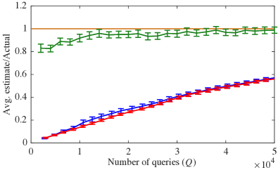
(a) email-EuAll

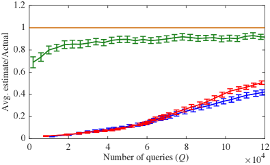
(b) com-Youtube

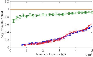
(c) loc-gowalla

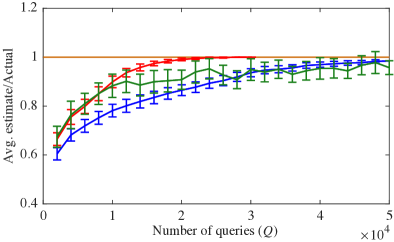
(d) com-Amazon

Figure 1: Comparison of the ratio of the average estimated value of $\lambda_{1}$ and the actual value. The brown line indicates 1. The error bars indicate 95% confidence intervals over 100 independent runs.

In this section, we present a performance analysis of cWalker-B and cWalker-C as described in Algorithm 2 and Algorithm 3. We compare our algorithms against two state-of-the-art algorithms, Spectral Radius Estimator (SRE) [33] and BackLink Count (BLC) [32]. We do not consider XS algorithm [31] in this analysis because, as already established in [33], it performs substantially poorer than both SRE and BLC. Both SRE and BLC aim to find a set of nodes which have the largest estimated eigenvalue centrality. They estimate the largest eigenvalue of the original graph by calculating the largest eigenvalue of the subgraph induced by the set of sampled nodes with high eigenvalue centrality.

Our experiments were performed on real graphs from the Stanford Network Analysis Project (SNAP) [37]. Table I lists some vital properties of these graphs. For each graph used, the algorithms were run on the largest connected component of the graph.

7.1 Results of estimating the largest eigenvalue

In this subsection, we show results of estimating the largest eigenvalue. We compare the cWalker-B algorithm (as described in Algorithm 2) against SRE and BLC. For all of the experiments of the cWalker-B algorithm, the accuracy target $\beta$ and the maximum length of closed walk $K$ were set to 0.05 and 30, respectively.

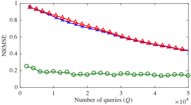
(a) email-EuAll

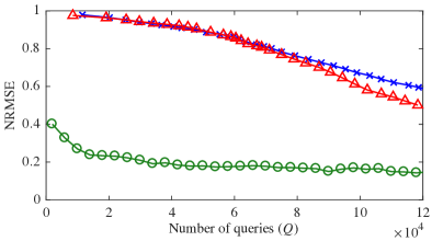
(b) com-Youtube

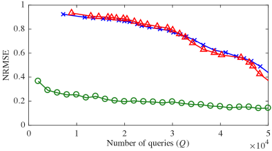
(c) loc-gowalla

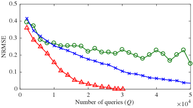
(d) com-Amazon

Figure 2: Comparison of NRMSEs of the estimates by the three algorithms.

As described in Section 4, the performance of our algorithm is affected by $\alpha$, the ratio of the second largest and the largest eigenvalue. The smaller the $\alpha$, the less information it needs to converge to an answer with acceptable accuracy. For the sake of completeness in our performance analysis, we demonstrate the rare case when $\alpha$ is extremely close to 1 by deliberately including the com-Amazon graph. Note that it is not common for real graphs to have an $\alpha$ extremely close to 1. In fact, in our study of 50 graphs listed on the SNAP site [37], com-Amazon graph had the highest value of $\alpha$ at 0.997. The $\alpha$ value of the other graphs, we found, were between 0.38 and 0.98, with a mean of 0.78 and a median of 0.82.

7.1.1 Accuracy

We consider the relative error as a measure of the accuracy. We measure the relative error as:

$$\mathrm{Relative~{}error}=\frac{\mathrm{Average~{}estimate}-\mathrm{Actual~{}value}}{\mathrm{Actual~{}value}},$$

where the average estimate is the mean of the estimated value across 100 independent runs. For each graph, we fixed $Q$, the number of queries, to ensure that all of the three algorithms obtain the same amount of information through its queries of the graph and to make sure that the evaluation is under equivalent complexity. The SRE algorithm is a greedy algorithm which keeps replacing the sampled nodes with more influential nodes after the size of the sample graph reaches the desired sample size. Here we set the desired size as 4% of the size of the original graph based on results in [33] which demonstrated a high accuracy at a sample size set to 4% of the full graph.

Table II shows the relative errors in estimating the largest eigenvalue for each of the three algorithms. The number of queries is $120$K for the com-Youtube graph and $50$K for the other graphs. As shown in the table, except for the case of the com-Amazon graph, the relative errors achieved by our algorithm are significantly better than BLC and SRE.

A further comparison of the three algorithms is shown in Fig. 1. It shows the ratio of the average estimated $\lambda_{1}$ to the actual value for each of the four graphs as the number of queries increased. As depicted in the figure, all of the algorithms gradually converge to the actual value. In the cases of the email-EuAll, com-Youtube and loc-gowalla graphs, our algorithm always achieves substantially better accuracy than BLC and SRE with increasing number of queries.

To provide a more comprehensive analysis of the accuracy of the three algorithms, we use the normalized root mean square error (NRMSE) which infers both the variance and the bias of the estimates. The NRMSE is defined as follows:

$$\mathrm{NRMSE}=\frac{\sqrt{\mathrm{E}[(\mathrm{estimate}-\mathrm{Actual~{}value})^{2}]}}{\mathrm{Actual~{}value}},$$

Fig. 2 plots the NRMSEs based on 100 independent runs for each graph with increasing number of queries. Similar to the results plotted in Fig. 1, our algorithm performs significantly better in terms of accuracy in the email-EuAll, com-Youtube and loc-gowalla graphs.

As expected, the com-Amazon graph is the only case for which our algorithm does not perform very well. We chose this graph as an exceptional case to show the influence of $\alpha$ on the performance of our algorithm. The ratio of $\lambda_{2}$ and $\lambda_{1}$, of the com-Amazon graph is extremely close to $1$. As listed in Table I, the largest and the second largest eigenvalue of the com-Amazon graph are 23.98 and 23.91, respectively. Thus, as plotted in Fig. 2(d), our algorithm has a larger variance and is less accurate in the com-Amazon graph. On the other hand, the com-Amazon graph has a small value of the largest eigenvalue which enables the BLC and the SRE algorithms to converge to the actual value quickly.

As summarized in [8], graphs which have high values of the largest eigenvalues usually have a small diameter, good expansion features and are more robust. Besides, the speed of propagation is higher in graphs with a large spectral gap, the difference between the first and second largest eigenvalues. Many social network graphs which are of primary interest in BigData graph analytics have a small diameter and good propagation properties; so, our algorithm is capable of achieving a good performance on such graphs.

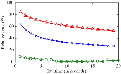
(a) email-EuAll

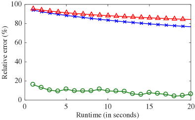
(b) com-Youtube

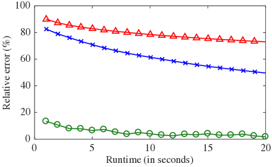
(c) loc-gowalla

(d) com-Amazon

Figure 3: Comparisons of the relative error in estimating the largest eigenvalue against the runtime in seconds.

7.1.2 Runtime

Both BLC and SRE try to sample the nodes with the largest eigenvalue centrality in the graph. They calculate and update the score of each neighboring node of the current sample set in order to select a node with the highest score. This leads to high computational complexity. The cWalker-B algorithm, on the other hand, achieves a significant improvement in the runtime by avoiding such score calculations and using the less computationally intensive method of a simple random walk.

We implemented the three algorithms, cWalker-B, BLC and SRE, in python using $networkx$ and $igraph$ modules. All of the simulations were run on an iMac with 16GB 1600MHz DDR3 memory and 2.7GHz Intel Core i5 processor. Here we assume that all of the graphs are stored on the local machine, so the query time is neglected.

Fig. 3 depicts the relative error of the estimate reached by the three algorithms against the runtime, averaged over 100 independent runs. As shown in the figure, the cWalker-B algorithm achieves much smaller relative errors for the same runtime. Of particular interest is the case of the com-Amazon graph, as plotted in Fig. 3(d), where it achieves better accuracy within the same runtime. This is in contrast to the earlier finding under the baseline of the number of queries (shown in Fig. 2(d)), where our algorithm achieves a lower accuracy given the same number of queries allowed. The cWalker-B algorithm is substantially faster than the other two algorithms because, given the same amount of runtime, it is able to process more information (visiting more nodes in the random walk) and achieve better accuracy.

7.2 Results of estimating the two largest eigenvalues

In this subsection, we show the results of estimating the two largest eigenvalues using the cWalker-C algorithm (as described in Algorithm 3). For all of the experiments evaluating this algorithm, the accuracy target $\beta$ and the maximum length of closed walk $K$ were set to 0.01 and 30, respectively.

Both SRE and BLC aim to collect a set of nodes which have the largest estimated eigenvalue centrality, and are not designed for estimating the second largest eigenvalue. However, based on interlacing results in spectral graph theory, where the eigenvalues of the full graph can be bounded using the eigenvalues of its subgraphs, the second largest eigenvalue of the sampled graph obtained by SRE and BLC can serve as a reference.

Fig. 4 depicts the ratio of the average estimated $\lambda_{1}$ and $\lambda_{2}$ to their actual values for each of the four graphs with increasing number of queries. Similar to the results of the cWalker-B algorithm, cWalker-C also cannot outperform the other two algorithms in the com-Amazon graph. Since the ratio of $\lambda_{2}$ and $\lambda_{1}$ of the com-Amazon graph is very close to 1, the value of $k$ used in the estimation is large. Thus, in the com-Amazon graph, our algorithm takes more steps to converge. Except for the case of the com-Amazon graph, the cWalker-C algorithm achieves substantially better accuracy than BLC and SRE in the estimation of both $\lambda_{1}$ and $\lambda_{2}$. As plotted in the figure, in the cases of the email-EuAll, loc-gowalla and com-Youtube graphs, the estimates of $\lambda_{2}$ obtained by our algorithm do not show a clear convergence towards the actual values (e.g., plots do not converge to the brown line). Especially in Fig. 4(c), we can see that the accuracy in estimating $\lambda_{2}$ becomes lower with the increasing number of queries. The reason why the estimates of $\lambda_{2}$ obtained by our algorithm do not converge towards the ground truth is that the value of $k$ used for estimating $\lambda_{2}$ is not large enough. As shown in Eqn. (4), when $k$ is not large enough, $\lambda_{1}$ and $\lambda_{2}$ cannot become the dominate terms in the RHS of this equation. In other words, the value of $\sum_{i=3}^{|V|}{\lambda_{i}}^{k}$ is unnegligible and makes the approximation of $\lambda_{2}$ be overestimated. Similar to the case of $\lambda_{1}$, the reasonable value of $k$ for estimating $\lambda_{2}$ depends on the ratio of $\lambda_{3}$ and $\lambda_{2}$. If this ratio is close to 1, the value of $k$ has to be very large in order to get an accurate estimate of $\lambda_{2}$. However, in our algorithm, we use the approximation of $\lambda_{1}$ to estimate $\lambda_{2}$, so the value of $k$ used in the estimation of $\lambda_{2}$ must be no larger than the one used to obtain the estimate of $\lambda_{1}$. For a graph where the ratio of $\lambda_{2}$ and $\lambda_{1}$ is small, while the ratio of $\lambda_{3}$ and $\lambda_{2}$ is large (e.g., close to 1), the approximation of $\lambda_{2}$ obtained by our algorithm can be overestimated due to the use of a small value of $k$. To avoid this situation, we can set the minimum value of $k$ to a relatively large value.

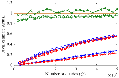
(a) email-EuAll

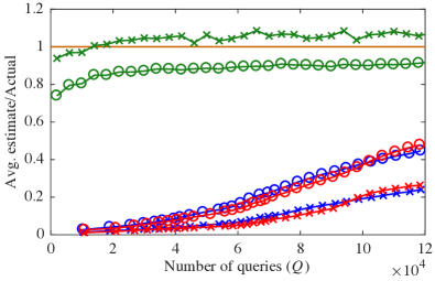
(b) com-Youtube

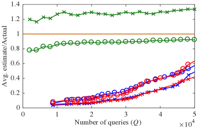
(c) loc-gowalla

(d) com-Amazon

Figure 4: Comparison of the ratio of the average estimated value of $\lambda_{1}$ and $\lambda_{2}$ to their actual values. The brown line indicates 1.

Fig. 5 plots the relative error of the estimates obtained by the three algorithms against the runtime, averaged over 100 independent runs. As plotted in the figure, the cWalker-C algorithm achieves much smaller relative errors under the same runtime. Similar to the results of the cWalker-B algorithm, the cWalker-C algorithm also achieves better accuracy within the same runtime in the com-Amazon graph. Combining with the results shown in Fig. 4(d), where our algorithm reaches a lower accuracy given the same number of queries allowed, we can say that the cWalker-C algorithm is faster than the other two algorithms. Moreover, as shown in Fig. 5(c), the relative error in estimating $\lambda_{2}$ obtained by our algorithm becomes larger with increasing amount of runtime. This is in line with the results shown in Fig. 4(c). The ratio of $\lambda_{2}$ and $\lambda_{1}$ of the loc-gowalla graph is 0.65, while its ratio of $\lambda_{3}$ and $\lambda_{2}$ is 0.95. The value of $k$ used for estimating $\lambda_{2}$ is not large enough, and thus leads to an overestimation of $\lambda_{2}$ in the case of the loc-gowalla graph.

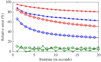
(a) email-EuAll

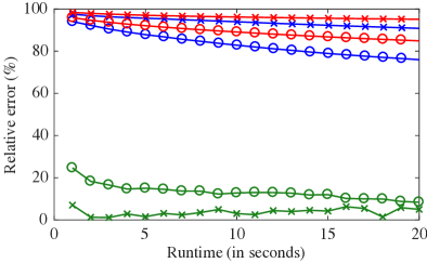
(b) com-Youtube

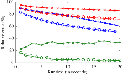
(c) loc-gowalla

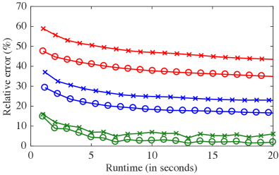
(d) com-Amazon

Figure 5: Comparison of the relative error in estimating the two largest eigenvalues against the runtime in seconds.

7.3 Complexity

TABLE III: The complexity of the algorithms.

Algorithm	Time complexity	Space complexity
cWalker-B	$O(t\log\Delta)$	$O(K+\Delta)$
cWalker-C	$O(t\Delta\log\Delta)$	$O(K\Delta)$
SRE	$O(n\Delta(s+\Delta))$	$O(s\Delta)$
BLC	$O(\Delta^{2}s^{3})$	$O(s\Delta)$

Besides accuracy, our algorithms achieve a much better performance in terms of the space complexity and the computational costs. Table III summaries the complexity of the algorithms.

7.3.1 Computational complexity

Denote by $\Delta$ the maximum degree of a node in the graph. The complexity of checking the occurrence of a node in the neighborhood of another node is $O(\log\Delta)$, assuming the neighbors of each node are stored in a sorted list. In the cWalker-B algorithm, at each step, we check if the node visited $k$ steps earlier is in the neighborhood of the current node; this leads to the complexity of $O(\log\Delta)$. For a random walk of length $t$, the complexity becomes $O(t\log\Delta)$. The cWalker-C algorithm needs to find common elements in the neighboring nodes of the first and the last nodes of a path; this takes $O(\Delta\log\Delta)$. So, its complexity is $O(t\Delta\log\Delta)$.

The runtime of SRE is highly influenced by the structure of the graph and the selection of the starting node. Every time the sample graph is updated, SRE updates the scores of all the corresponding nodes, which can consume significant time for graphs with high average node degree. SRE is a greedy algorithm, so the selection of the starting node is especially determinative of the runtime. As presented in [33], SRE takes $O(s\Delta+\Delta^{2})$ to select one node for removal from the sample subgraph and one node for addition into it, where $s$ is the size of the sample graph. In the worst case, SRE may have to visit the entire graph in order to make an estimate with sufficient accuracy which leads to a complexity of $O(n\Delta(s+\Delta))$.

BLC adopts a different metric to compute the score of the nodes, using the number of neighbors of a node in the sample graph (unlike SRE which uses the sum of the degrees of the node’s neighbors.) The complexity of the BLC algorithm, as described in [32], is $O(\Delta^{2}s^{3})$.

7.3.2 Space complexity

For the cWalker-B algorithm, as we visit nodes in the random walk, we keep checking if one of the neighboring nodes of the current node is identical to the previously visited node $k-1$ steps earlier. So we only need to store the neighborhood information of one node and track up to $k$ steps of the random walk. The cWalker-B algorithm has a space complexity of $O(K+\Delta)$, where $K$ is the maximum length of closed walk being checked in the algorithm. Note that $K$ is a small constant which is accepted as an input. As for the cWalker-C algorithm, we need to check the number of common neighbors between the first and the last node in paths of length $k-2$. To avoid querying the neighboring nodes of previously visited nodes again, the neighborhood information of previously visited $k-2$ nodes are stored. So the space complexity is $O(K\Delta)$

For the BLC and SRE algorithms, however, at each step, both of them need to pick up a node which has the highest score from the neighborhood of the current sample graph, so they have to store both the sample graph and the score of each neighboring node of the current sample graph which leads to a complexity of $O(s\Delta)$.

8 Conclusion

In this paper, we present a series of new sampling algorithms which estimate the largest and the second largest eigenvalues of the graph. Unlike previous methods which seek out nodes with high eigenvalue centrality based on some score, our algorithm achieves a significant improvement in computational efficiency by adopting an entirely different approach. Our method is based on estimating the number of closed walks of length $k$ by exploiting its relationship to the $k$-th spectral moment of the graph. Our results demonstrate that, on most graphs, our algorithms achieve substantially better accuracy at a lower computational cost than previously known algorithms.

Random walks on graphs had previously been used by graph sampling algorithms to ascertain simple properties of graphs such as its clustering co-efficient, motif statistics or centrality measures. This paper offers hope that random walks can indeed be employed to sample and estimate complex properties of graphs such as its eigenvalues.

References

- [1] F. Chung, Spectral graph theory. American Mathematical Society, 1997.
- [2] M. Cohn, “On the channel capacity of read/write isolated memory,” Discrete applied mathematics, vol. 56, no. 1, pp. 1–8, 1995.
- [3] Y. Hong, “Bounds of eigenvalues of graphs,” Discrete Mathematics, vol. 123, no. 1-3, pp. 65–74, 1993.
- [4] D. M. Cvetković, P. Rowlinson, and S. Simic, Eigenspaces of graphs. Cambridge University Press, 1997, no. 66.
- [5] S. Brin and L. Page, “The anatomy of a large-scale hypertextual web search engine,” Computer Networks and ISDN Systems, vol. 30, no. 1-7, pp. 107–117, 1998.
- [6] F. Chung and L. Lu, Complex Graphs and Networks. American Mathematical Society, 2006.
- [7] Y. Wang, D. Chakrabarti, C. Wang, and C. Faloutsos, “Epidemic spreading in real networks: An eigenvalue viewpoint,” in Proceedings of the 22nd International Symposium on Reliable Distributed Systems. IEEE, 2003, pp. 25–34.
- [8] P. Mahadevan, D. Krioukov, M. Fomenkov, X. Dimitropoulos, A. Vahdat et al., “The Internet AS-level topology: three data sources and one definitive metric,” ACM SIGCOMM Computer Communication Review, vol. 36, no. 1, pp. 17–26, 2006.
- [9] L. Lovász, “Random walks on graphs,” Combinatorics, Paul erdos is eighty, vol. 2, no. 1-46, p. 4, 1993.
- [10] A. E. Brouwer and W. H. Haemers, Spectra of graphs. Springer Science & Business Media, 2011.
- [11] B. Noble and J. W. Daniel, Applied linear algebra. Prentice-Hall New Jersey, 1988, vol. 3.
- [12] G. Han and H. Sethu, “Closed walk sampler: An efficient method for estimating the spectral radius of large graphs,” in Proceedings of IEEE International Conference on Big Data. IEEE, 2017, pp. 616–625.
- [13] J. Kuczyński and H. Woźniakowski, “Estimating the largest eigenvalue by the power and Lanczos algorithms with a random start,” SIAM journal on matrix analysis and applications, vol. 13, no. 4, pp. 1094–1122, 1992.
- [14] K.-J. Bathe and E. L. Wilson, Numerical methods in finite element analysis. Prentice-Hall Englewood Cliffs, NJ, 1976, vol. 197.
- [15] G. Peters and J. H. Wilkinson, “Inverse iteration, ill-conditioned equations and newton’s method,” SIAM Review, vol. 21, no. 3, pp. 339–360, 1979.
- [16] B. N. Parlett, “The Rayleigh quotient iteration and some generalizations for nonnormal matrices,” Mathematics of Computation, vol. 28, no. 127, pp. 679–693, 1974.
- [17] J. H. Wilkinson and J. H. Wilkinson, The algebraic eigenvalue problem. Clarendon Press Oxford, 1965, vol. 87.
- [18] K.-J. Bathe and E. L. Wilson, “Solution methods for eigenvalue problems in structural mechanics,” International Journal for Numerical Methods in Engineering, vol. 6, no. 2, pp. 213–226, 1973.
- [19] K.-J. Bathe and S. Ramaswamy, “An accelerated subspace iteration method,” Computer Methods in Applied Mechanics and Engineering, vol. 23, no. 3, pp. 313–331, 1980.
- [20] I. C. Ipsen, “Computing an eigenvector with inverse iteration,” SIAM Review, vol. 39, no. 2, pp. 254–291, 1997.
- [21] M. Panju, “Iterative methods for computing eigenvalues and eigenvectors,” https://arxiv.org/abs/1105.1185, 2011.
- [22] Y. Hong, J.-L. Shu, and K. Fang, “A sharp upper bound of the spectral radius of graphs,” Journal of Combinatorial Theory, Series B, vol. 81, no. 2, pp. 177–183, 2001.
- [23] R. P. Stanley, “A bound on the spectral radius of graphs with e edges,” Linear Algebra and its Applications, vol. 87, pp. 267–269, 1987.
- [24] V. Nikiforov, “Walks and the spectral radius of graphs,” Linear Algebra and its Applications, vol. 418, no. 1, pp. 257–268, 2006.
- [25] K. C. Das and P. Kumar, “Some new bounds on the spectral radius of graphs,” Discrete Mathematics, vol. 281, no. 1, pp. 149–161, 2004.
- [26] D. Cvetković and S. Simić, “The second largest eigenvalue of a graph (a survey),” Filomat, pp. 449–472, 1995.
- [27] G. Han and H. Sethu, “Waddling random walk: Fast and accurate mining of motif statistics in large graphs,” in Proceedings of the 16th IEEE International Conference on Data Mining. IEEE, 2016, pp. 181–190.
- [28] M. Jha, C. Seshadhri, and A. Pinar, “A space efficient streaming algorithm for triangle counting using the birthday paradox,” in Proceedings of the 19th ACM SIGKDD International Conference on Knowledge Discovery and Data Mining. ACM, 2013, pp. 589–597.
- [29] P. Wang, J. C. Lui, D. Towsley, and J. Zhao, “Minfer: A method of inferring motif statistics from sampled edges,” in Proceedings of the 32nd IEEE International Conference on Data Engineering. IEEE, 2016, pp. 1050–1061.
- [30] N. K. Ahmed, N. Duffield, J. Neville, and R. Kompella, “Graph sample and hold: A framework for big-graph analytics,” in Proceedings of the 20th ACM SIGKDD International Conference on Knowledge Discovery and Data Mining. ACM, 2014, pp. 1446–1455.
- [31] A. Maiya and T. Berger-Wolf, “Online sampling of high centrality individuals in social networks,” Advances in Knowledge Discovery and Data Mining, pp. 91–98, 2010.
- [32] J. Cho, H. Garcia-Molina, and L. Page, “Efficient crawling through URL ordering,” Computer Networks and ISDN Systems, vol. 30, no. 1, pp. 161–172, 1998.
- [33] X. Chu and H. Sethu, “On estimating the spectral radius of large graphs through subgraph sampling,” in Proceedings of IEEE Conference on Computer Communications Workshops (INFOCOM WKSHPS). IEEE, 2015, pp. 432–437.
- [34] S. J. Hardiman and L. Katzir, “Estimating clustering coefficients and size of social networks via random walk,” in Proceedings of the 22nd International Conference on World Wide Web, 2013, pp. 539–550.
- [35] L. Katzir, E. Liberty, and O. Somekh, “Estimating sizes of social networks via biased sampling,” in Proceedings of the 20th International Conference on World Wide Web. ACM, 2011, pp. 597–606.
- [36] S. J. Hardiman, P. Richmond, and S. Hutzler, “Calculating statistics of complex networks through random walks with an application to the on-line social network bebo,” The European Physical Journal B-Condensed Matter and Complex Systems, vol. 71, no. 4, pp. 611–622, 2009.
- [37] J. Leskovec and A. Krevl, “SNAP Datasets: Stanford large network dataset collection,” http://snap.stanford.edu/data, Jun. 2014.