Photon entanglement entropy as a probe of many-body correlations and fluctuations

Abstract

Recent theoretical and experiments have explored the use of entangled photons as a spectroscopic probe of material systems. We develop here a theoretical description for entropy production in the scattering of an entangled biphoton state within an optical cavity. We develop this using perturbation theory by expanding the biphoton scattering matrix in terms of single-photon terms in which we introduce the photon-photon interaction via a complex coupling constant, $\xi$. We show that the von Neumann entropy provides a succinct measure of this interaction. We then develop a microscopic model and show that in the limit of fast fluctuations, the entanglement entropy vanishes whereas in the limit the coupling is homogeneous broadened, the entanglement entropy depends upon the magnitude of the fluctuations and reaches a maximum.

I Introduction

Dynamical light scattering provides a sensitive probe of correlations and fluctuations in material systems. The basic theory and first applications of this technique harken back to experiments by Tyndall on aerosols in the 1860’s and theoretical work by Rayleigh.Tyndall (1869a, 1863, b); Lord Rayleigh (1871a) (Strutt, J. W.); Lord Rayleigh (1871b) (Strutt, J. W.); Lord Rayleigh (1871c) (Strutt, J. W.) In fact, Rayleigh showed that light scattering from density fluctuations in the atmosphere give rise to the blue color of the sky.Lord Rayleigh (1899) (Strutt, J. W.) The classic text by Berne and Pecorra helped to establish the modern theory of dynamical light scattering as an important probe of chemical physical processes.Berne and Pecora (1976)

Experiments using entangled photon pairs as probes of material systems have opened a new arena for both linear and non-linear spectroscopy since quantum entangled photons facilitate a direct probe of many-body correlations. Ladd et al. (2010); Lemos et al. (2014); Gisin et al. (2002); Sewell (2017); Zou, Wang, and Mandel (1991); Roslyak, Marx, and Mukamel (2009); Schlawin et al. (2013); Li et al. (2018) With this in mind, we develop here a theoretical approach that connects the resultant entropic change within a biphoton state to the matter-mediated coupling between the photons within the sample. Our theory develops from a perturbative expansion of the biphoton amplitude in which the single-photon terms are coupled order-by-order via a a complex entanglement parameter, $\xi$, which we take as a measure of the photon-photon coupling mediated by the medium. We also develop a microscopic model for photon-photon entanglement a mediated by cross-correlated spectral fluctuations and relate this to the von Neumann entropy of the outgoing biphoton quantum state. We show that in the limit of rapid fluctuations and motional narrowing destroy entanglement whereas in the limit of homogeneous broadening (gaussian noise), fluctuations produce entangled states with a maximum entropy determined by the spectral width.

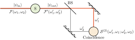
Figure 1: Spectrally-resolved Hanbury Brown and Twiss experimental setup. Following the beam-splitter (BS), the two photon frequencies are resolved before coincidence detection.

II Diagrammatic representation of two-photon scattering amplitude

As illustrated in Fig. 1, we consider here the entanglement produced by the interaction of an initial biphoton input stateLoudon (2000a)

$$|\psi_{\text{in}}\rangle = \iint d\omega_{1}d\omega_{2}{\cal F}(\omega_{1},\omega_{2})\hat{B}^{\dagger}(\omega_{1})\hat{B}^{\dagger}(\omega_{2})|0\rangle$$ (1)

with a sample $S$ to produce a biphoton output state

$$|\psi_{\text{out}}\rangle = \iint d\omega^{\prime}_{1}d\omega^{\prime}_{2}\iint d\omega_{1}d\omega_{2}$$

$${\cal S}^{(2)}(\omega_{1},\omega_{2};\omega^{\prime}_{1},\omega^{\prime}_{2}){\cal F}(\omega_{1},\omega_{2})\hat{B}^{\dagger}(\omega_{1})\hat{B}^{\dagger}(\omega_{2})|0\rangle$$

Here, we denote photon creation operators $\hat{B}^{\dagger}(\omega_{1})$ and $\hat{B}^{\dagger}(\omega_{2})$ acting on the photon vacuum state $|0\rangle$, and the scattering amplitude ${\cal S}^{(2)}$ reflecting the photons interaction with the sample. We shall leave the exact representation of the scattering amplitude undefined at the moment; however, we assume throughout that interaction with the sample placed before the beam-splitter affects the two-photon entanglement as the result of many-body interactions occurring when two photons interact with each other via the medium. In principle, initial input ${\cal F}(\omega_{1},\omega_{2})$ may be separable into single photon terms ${\cal F}(\omega_{1},\omega_{2})=f_{1}(\omega_{1})f_{2}(\omega_{2})$ but we shall assume that the output amplitude is not separable and corresponds to an entangled photon pair.

Following interaction with the sample, the light passes through a symmetrical beam splitter (BS). For co-linear photon beams, this produces the mappingLoudon (2000a); Li et al. (2018)

$$\hat{B}^{\dagger}(\omega^{\prime}_{1})\hat{B}^{\dagger}(\omega^{\prime}_{2})\mapsto\frac{1}{2}[\hat{A}^{\dagger}_{1}(\omega^{\prime}_{1})+i\hat{A}^{\dagger}_{2}(\omega^{\prime}_{1})][\hat{A}^{\dagger}_{1}(\omega^{\prime}_{2})+i\hat{A}^{\dagger}_{2}(\omega^{\prime}_{2})],$$ (3)

where $A^{\dagger}_{1}$ ($A^{\dagger}_{2}$) creates a photon state in channel 1 (channel 2) after the beam splitter resulting in the post-beam splitter state given by

$$|\psi_{BS}\rangle = \frac{1}{2}\left(|\psi_{1}\rangle-|\psi_{2}\rangle+|\psi_{c}\rangle\right)$$ (4)

where the kets $|\psi_{1}\rangle$ and $|\psi_{2}\rangle$ correspond to the cases where both photons are in either channel, and

$$|\psi_{c}\rangle = \frac{i}{2}\iint d\omega^{\prime}_{1}d\omega^{\prime}_{2}\iint d\omega_{1}d\omega_{2}{\cal S}^{(2)}(\omega_{1},\omega_{2};\omega^{\prime}_{1},\omega^{\prime}_{2}){\cal F}(\omega_{1},\omega_{2})[\hat{A}_{1}^{\dagger}(\omega_{1})\hat{A}_{2}^{\dagger}(\omega_{2})+\hat{A}_{2}^{\dagger}(\omega_{1})\hat{A}_{1}^{\dagger}(\omega_{2})]|0\rangle$$ (5)

$$= \frac{i}{2}\iint d\omega^{\prime}_{1}d\omega^{\prime}_{2}\iint d\omega_{1}d\omega_{2}[{\cal S}^{(2)}(\omega_{1},\omega_{2};\omega^{\prime}_{1},\omega^{\prime}_{2}){\cal F}(\omega_{1},\omega_{2})+{\cal S}^{(2)}(\omega_{2},\omega_{1};\omega^{\prime}_{2},\omega^{\prime}_{1}){\cal F}(\omega_{2},\omega_{1})]|\omega_{1}\omega_{2}\rangle$$ (6)

corresponds to the case where single photons are in both channels leading to the possibility of detecting the coincidence counts. From this we compute the coincidence probability as

$$P_{c}=\langle\psi_{c}|\psi_{c}\rangle= \frac{1}{4} \iint d\omega_{1}d\omega_{2}\iint d\omega_{1}^{\prime}d\omega_{2}^{\prime}\{|{\cal S}^{(2)}(\omega_{1},\omega_{2};\omega_{1}^{\prime},\omega_{2}^{\prime})|^{2}|{\cal F}(\omega_{1},\omega_{2})|^{2}+|{\cal S}^{(2)}(\omega_{2},\omega_{1};\omega_{2}^{\prime},\omega_{1}^{\prime})|^{2}|{\cal F}(\omega_{2},\omega_{1})|^{2}$$ (7)

$$+ 2\mathrm{Re}[{\cal S}^{(2)}(\omega_{1},\omega_{2};\omega_{1}^{\prime},\omega_{2}^{\prime}){\cal F}(\omega_{1},\omega_{2}){\cal S}^{(2)*}(\omega_{2},\omega_{1};\omega_{2}^{\prime},\omega_{1}^{\prime}){\cal F}^{*}(\omega_{2},\omega_{1})]\}$$ (8)

which we take to be the integrated number of coincident photon pairs counted per unit time. For the experimental set-up sketched in Fig. 1, symmetry dictates that ${\cal S}^{(2)}(\omega_{1},\omega_{2};\omega_{1}^{\prime},\omega_{2}^{\prime})={\cal S}^{(2)}(\omega_{2},\omega_{1};\omega_{2}^{\prime},\omega_{1}^{\prime})$ and ${\cal F}(\omega_{1},\omega_{2})={\cal F}(\omega_{2},\omega_{1})$, leading to a counting rate of

$$P_{c}=\iint d\omega_{1}d\omega_{2}\iint d\omega_{1}^{\prime}d\omega_{2}^{\prime}|{\cal F}(\omega_{1},\omega_{2})|^{2}|{\cal S}^{(2)}(\omega_{1},\omega_{2};\omega^{\prime}_{1},\omega^{\prime}_{2})|^{2}.$$ (9)

Hence, by measuring the spectral or polarization resolved coincidences, one can reconstruct the biphoton scattering probability. We next develop a relation between the scattered biphoton amplitude ${\cal S}^{(2)}$ and the spectral response of the system.

II.1 Diagrammatic Expansion of Scattering Amplitude

In general, we can write the elastic scattering of a single photon through a resonant medium in the form

$${\cal S}^{(1)}(\omega,\omega^{\prime})=\exp({\cal A}(\omega))\delta(\omega-\omega^{\prime})$$ (10)

where

$${\cal A}(\omega)=-\frac{ib}{(\omega_{o}-\omega)+i\gamma}$$ (11)

is the Fourier transform of the free induction decay

$${\cal A}(t)=-\sqrt{2\pi}be^{-\gamma t}e^{i\omega_{o}t}$$ (12)

for $t>0$ of an oscillator with frequency $\omega_{o}$ and dephasing time $1/\gamma$. $b=\alpha L\gamma/2$ where $\alpha L$ is the optical thickness and $\alpha$ is a Bouger coefficient. Consequently, if two independent (non-entangled) photons are scattered from the resonant medium we anticipate a scattering amplitude of

$${\cal S}^{(2)}(\omega_{1},\omega_{2};\omega^{\prime}_{1},\omega^{\prime}_{2})={\cal S}^{(1)}(\omega_{1}){\cal S}^{(1)}(\omega_{2})\delta(\omega_{1}-\omega_{1}^{\prime})\delta(\omega_{2}-\omega_{2}^{\prime})$$ (13)

In this case, two independent photons are transmitted without any interaction leading to them being entangled.

Suppose, however, that interactions leading to entanglement are weak such that we can write the two photon scattering amplitude as perturbation expansion of the form

$${\cal S}^{(2)} = {\cal S}^{(2)}_{o}+{\cal S}_{o}^{(2)}{\cal V}{\cal S}^{(2)}={\cal S}^{(2)}_{o}+{\cal S}_{o}^{(2)}{\cal V}{\cal S}_{o}^{(2)}+{\cal S}_{o}^{(2)}{\cal V}{\cal S}_{o}^{(2)}{\cal V}{\cal S}_{o}^{(2)}+\cdots$$

whereby ${\cal S}^{(2)}_{o}={\cal S}^{(1)}{\cal S}^{(1)}$ is separable into single photon terms and ${\cal V}$ mediates the interaction between photon pairs via the resonant cavity. This suggests the following diagrammatic expansion

(14)

where solid lines are ${\cal S}^{(1)}$ propagations and springs denote the interaction. Suppose we write that ${\cal V}(\omega)$ contributes a phase-shift of the form

$${\cal V}(\omega)=\xi e^{i\phi}\delta(\omega)$$ (15)

but does not create a frequency shift. Then only the term at $\omega=0$ will contribute (so that $\omega_{1}=\omega_{1}^{\prime}$ and $\omega_{2}=\omega_{2}^{\prime}$)

$${\cal S}_{1}^{(2)}=\xi e^{i\phi}{\cal S}^{(1)}(\omega_{1}){\cal S}^{(1)}(\omega_{2}){\cal S}^{(1)}(\omega_{1}){\cal S}^{(1)}(\omega_{2})$$ (16)

Iterating this,

$${\cal S}_{n}^{(2)} = {\cal V}^{n}\left({\cal S}_{o}^{(2)}\right)^{n+1}=\xi^{n}e^{in\phi}\left({\cal S}^{(1)}(\omega_{1})\right)^{n+1}\left({\cal S}^{(1)}(\omega_{2})\right)^{n+1}$$ (17)

Taking

$${\cal S}^{(1)}(\omega_{i})=\exp\left[-\frac{ib}{(\omega_{o}-\omega_{i})+i\gamma}\right]=z_{i}$$ (18)

is a complex number determined by the input photon frequency. Thus, the whole perturbation series becomes

$${\cal S}^{(2)}=z_{1}z_{2}\sum_{n=0}^{\infty}\left(\xi e^{i\phi}z_{1}z_{2}\right)^{n}$$ (19)

Setting $q=\xi e^{i\phi}z_{1}z_{2}$ and assuming $|q|<1$ then the series can be summed exactly

$${\cal S}^{(2)}=\frac{z_{1}z_{2}}{1-q}$$ (20)

Writing this in terms of the ${\cal S}^{(1)}$ functions, we obtain

$${\cal S}^{(2)}(\omega_{1},\omega_{2};\omega_{1},\omega_{2})=\frac{{\cal S}^{(1)}(\omega_{1}){\cal S}^{(1)}(\omega_{2})}{1-\xi{\cal S}^{(1)}(\omega_{1}){\cal S}^{(1)}(\omega_{2})e^{i\phi}}.$$ (21)

We shall refer to $\xi$ as the entanglement parameter. When $\xi=0$,

$${\cal S}^{(2)}(\omega_{1},\omega_{2})=\exp[{\cal A}^{(1)}(\omega_{1})]\exp[{\cal A}^{(1)}(\omega_{2})]={\cal S}^{(1)}(\omega_{1}){\cal S}^{(1)}(\omega_{2})$$ (22)

is separable in terms of the individual photon amplitudes.

II.2 Averaging over Phase

In principle, the phase $\phi$ introduced in Eq. 15 depends upon the microscopic details of the system, such as the relative orientation of the atomic or molecular scattering sites within the sample, and may be simply be a random quantity. Averaging over phase, we write

$$\overline{\cal S}^{(2)}(\omega_{1},\omega_{2};\omega_{1},\omega_{2})=\left\langle\frac{{\cal S}^{(1)}(\omega_{1}){\cal S}^{(1)}(\omega_{2})}{1-\xi{\cal S}^{(1)}(\omega_{1}){\cal S}^{(1)}(\omega_{2})e^{i\phi}}\right\rangle.$$ (23)

Writing this again as a geometric series

$$\overline{\cal S}^{(2)}(\omega_{1},\omega_{2};\omega_{1},\omega_{2})={\cal S}^{(1)}(\omega_{1}){\cal S}^{(1)}(\omega_{2})\sum_{n}(\xi{\cal S}^{(1)}(\omega_{1}){\cal S}^{(1)}(\omega_{2}))^{n}\left\langle e^{in\phi}\right\rangle.$$ (24)

Suppose that the phase $\phi$ is uniform over $[0,2\pi)$, then

$$\left\langle e^{in\phi}\right\rangle=\int_{0}^{2\pi}\frac{e^{in\phi}}{2\pi}d\phi=\delta_{n0}.$$

In this case, the relative phase is completely randomized and the biphoton amplitude collapses exactly into the product of two single photon terms.

$$\overline{\cal S}^{(2)}(\omega_{1},\omega_{2};\omega_{1},\omega_{2})\to{\cal S}^{(1)}(\omega_{1}){\cal S}^{(1)}(\omega_{2})$$ (25)

On the other hand, suppose the phase is normally distributed about a central value, which we can take to be zero, i.e. $\overline{\phi}=0$ and $\overline{\phi^{2}}=\sigma^{2}$. Here, the average over $\phi$ can be cast as

$$\left\langle e^{in\phi}\right\rangle=\left(1-\frac{n^{2}\overline{\phi^{2}}}{2!}+\frac{n^{4}\overline{\phi^{4}}}{4!}-\cdots\right)$$

Writing this in terms of the second moment

$$\left\langle e^{in\phi}\right\rangle=\sum_{k=0}^{\infty}(-1)^{k}(n\sigma)^{2k}\frac{(2k-1)!!}{(2k)!}=\sum_{k=0}^{\infty}(-1)^{k}\frac{(n\sigma)^{2k}}{2^{k}k!}=e^{-(n\sigma)^{2}/2}.$$ (26)

This gives

$$\overline{\cal S}^{(2)}(\omega_{1},\omega_{2};\omega_{1},\omega_{2})=\sum_{n=0}^{\infty}\xi^{n}e^{-n^{2}\sigma^{2}/2}({\cal S}^{(1)}(\omega_{1}){\cal S}^{(1)}(\omega_{2}))^{n+1}.$$ (27)

Plots for this are shown in Fig. 2a for the case of a model system with spectral parameters for Eq. (18): $\omega_{0}=\pi$, $b_{o}=1$ and $\gamma=2$. In each case, we assume an input of two photon Fock-state giving an output biphoton amplitude that is correlated along $\omega_{1}=\omega_{2}$. For the case of Gaussian noise, the final state is not necessarily separable into the product of two functions and the resulting state is correlated in frequency, as shown in Fig. 2 for various choices of spectral parameters. The von Neumann entropy, $S_{\psi}$ (c.f. Sec. III.2) gives a useful means of quantifying the entanglement of these states. Schmidt decomposition of Eq. 27 for a given value of $\sigma$ gives Fig. 2b where we have plotted the von Neumann entropy in terms of increasing interaction and in terms of increasing Gaussian noise. Generally, increasing $\xi$ leads to an increase in entanglement for a given amount of noise $\sigma$ as shown in Fig. 2b.

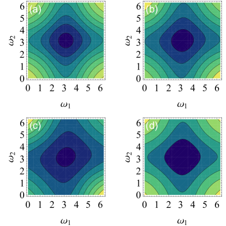
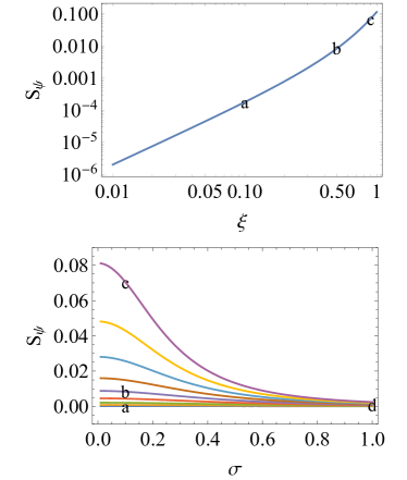
Figure 2: (Left) Absolute values of two-photon scattering functions for squeezed biphotons with Gaussian noise interactions: (a) $\xi=0.1$, $\sigma=0.1$; (b) $\xi=0.5$, $\sigma=0.1$; (c) $\xi=0.9$, $\sigma=0.1$; (d) $\xi=0.5$, $\sigma=1.0$. In each case we take parameters for ${\cal S}^{(1)}$ in Eq. (18) as: $\omega_{0}=\pi$, $b_{o}=1$ and $\gamma=2$. (Right,top) Entanglement entropy (Eq. (54)) vs. coupling $\xi$ for case of gaussian noise. Points a,b, and c correspond to specific biphoton states shown to the left. (Right,bottom) Entanglement entropy (Eq. (54)) vs. noise strength ($\sigma$). Points a to d correspond to specific biphoton states shown to the left.

III Stochastic model for two-photon scattering amplitude and entanglement entropy

We now dig deeper and develop a fully microscopic model for entropy production in biphoton scattering. In time-domain the input state on the left boundary of the cavity (Fig. 1) can be represented as

$$|\psi_{\text{in}}\rangle=\iint dt_{1}dt_{2}{\cal F}(t_{1},t_{2})\hat{b}_{1,\text{in}}^{\dagger}(t_{1})\hat{b}_{2,\text{in}}^{\dagger}(t_{2})|0\rangle,$$ (28)

where the cavity input photon operatorLi et al. (2018)

$$\hat{b}^{\dagger}_{j,\text{in}}(t)=-\int\frac{d\omega}{\sqrt{2\pi}}\hat{B}_{j}^{\dagger}(\omega)e^{i\omega t}$$ (29)

is the Fourier transform of the external photon mode operator $\hat{B}_{j}^{\dagger}(\omega)$ entering Eq. (1). Noteworthy that substitution of Eq. (29) into Eq. (28) and subsequent integration over the time variables exactly results in the frequency domain representation given by Eq. (1) where ${\cal F}(\omega_{1},\omega_{2})$ is identified as the Fourier transform of ${\cal F}(t_{1},t_{2})$. Following, the input output formalism,Gardiner and Savage (1984); Collett and Gardiner (1984) we identify the boundary condition on the left boundary of the cavity with the mode leakage rate $\kappa_{j}$ as $\hat{b}_{j,\text{in}}^{\dagger}(t)+\hat{b}_{j,\text{r}}^{\dagger}(t)=\sqrt{\kappa_{j}}\hat{b}_{j}^{\dagger}(t)$. This connects the input photon operator defined above, the reflected (output) photon operator $\hat{b}_{j,\text{r}}^{\dagger}(t)$, and the cavity photon operator $b_{j}^{\dagger}(t)$. The reflected mode is not measured in experiment and will not be considered below. However, the cavity mode operator contains information on the interactions within the cavity and will be determined below.

Time domain cavity output operators can be expressed in terms of the photon operators outside the cavity as Li et al. (2018)

$$\hat{b}^{\dagger}_{j,\text{out}}(t)=\int\frac{d\omega}{\sqrt{2\pi}}\hat{B}_{j}^{\dagger}(\omega)e^{i\omega(t-t_{f})},$$ (30)

representing interaction free photon modes $\hat{B}_{j}^{\dagger}(\omega)$ outside the cavity propagated back in time from $t_{f}$ to actual measurement time $t$. Evaluation of the coincidence probability requires partitioning of $\hat{B}_{j}^{\dagger}(\omega)$ operator according to Eq. (3). Thus, the output state needs to be represented in terms of these operators as $|\psi_{\text{out}}\rangle=\iint d\omega^{\prime}_{1}d\omega^{\prime}_{2}{\cal F}(\omega^{\prime}_{1},\omega^{\prime}_{2})\hat{B}_{1}^{\dagger}(\omega^{\prime}_{1})\hat{B}_{2}^{\dagger}(\omega^{\prime}_{2})|0\rangle$ which according Eq. (30) translates to

$$|\psi_{\text{out}}\rangle = \iint d\omega_{1}d\omega_{2}{\cal F}(\omega_{1},\omega_{2})\iint dt_{1}dt_{2}e^{-i\omega_{1}(t_{1}-t_{f})}$$

$$\times e^{-i\omega_{2}(t_{2}-t_{f})}\langle\hat{b}_{1,\text{out}}^{\dagger}(t_{1})\hat{b}_{2,\text{out}}^{\dagger}(t_{2})\rangle|0\rangle,\;\;\;\;$$

where and angle brackets describe the average of the output operators over the material induced cavity mode fluctuations. Similar to the input mode we establish the following boundary condition on the cavity right boundary $\hat{b}_{j,\text{out}}^{\dagger}(t)=\sqrt{\kappa_{j}}\hat{b}_{j}^{\dagger}(t)$. This condition assumes the same cavity leakage, $\kappa_{j}$, and according to the setup geometry in Fig. 1, no input photons on the right. Taking into account this boundary condition, evaluation of the output state using Eq. (III) reduces to the evaluation of the time domain correlation function of the cavity mode operators that will directly result in the evaluation of the desired scattering amplitude.

III.1 Stochastic Model for Cavity Photon Scattering

We adopt the following stochastic Hamiltonian to describe cavity photon modes $\hat{b}_{j}^{\dagger}$ coupled to the input and output biphoton states

$$\hat{H}_{\text{ph}}=\hbar\sum\limits_{j=1,2}\left(\omega_{j}+\delta\omega_{j}\right)\hat{b}_{j}^{\dagger}\hat{b}_{j}.$$ (32)

Here, $\delta\omega_{j}=\delta\omega_{j}(t)$ is the time-dependent photon frequency fluctuations of each mode. Appendix A provides an example connecting such a generic Hamiltonian with a microscopic Hamiltonian describing photon wave packet scattering by fluctuations of delocalized polariton modes confined within a cavity.

Applying input output formalism to the cavity modes described by the Hamiltonian (32), one obtains the quantum Langevin equationGardiner and Collett (1985); Li et al. (2018)

$$\frac{\partial}{\partial t}\hat{b}_{j}^{\dagger}(t)=i\left(\tilde{\omega}_{j}+\delta\omega_{j}\right)\hat{b}_{j}^{\dagger}(t)+\sqrt{\kappa_{j}}\hat{b}_{j,\text{in}}^{\dagger}(t).$$ (33)

with $\tilde{\omega}_{j}=\omega_{j}+i\kappa_{j}/2$. Assuming that the material fluctuation dynamics occurs on the timescale faster that the cavity leakage one can formally integrate Eq. (33) that results in

$$\hat{b}_{j,\text{out}}^{\dagger}(t) = \sqrt{\kappa_{j}}\int_{0}^{t}dt^{\prime}e^{i\tilde{\omega}_{j}(t-t^{\prime})}$$

$$\times \exp_{+}\left[i\int\limits_{t^{\prime}}^{t}d\tau\delta\omega_{j}(\tau)\right]\hat{b}_{j,\text{in}}^{\dagger}(t^{\prime}),$$

with $\exp_{+}[\dots]$ being positive time ordered exponential. Here, we also used the boundary condition for the cavity right boundary to express the cavity mode operator in terms of cavity output mode.

According to Eq. (III.1), the output single and two-photon operators averaged over the cavity fluctuations can be represented as

$$\langle\hat{b}_{j,\text{out}}^{\dagger}(t)\rangle=\int_{0}^{\infty}dt^{\prime}{\cal S}_{j}^{(1)}(t,t^{\prime})f_{j}(t^{\prime})\hat{b}_{\text{in},j}^{\dagger}(t^{\prime}),$$ (35)

$$\langle\hat{b}_{1,\text{out}}^{\dagger}(t_{1})\hat{b}_{2,\text{out}}^{\dagger}(t_{2})\rangle=\int_{0}^{\infty}dt_{1}^{\prime}\int_{0}^{\infty}dt_{2}^{\prime}$$

$$\hskip 20.0pt{\cal S}^{(2)}(t_{1}t_{2},t_{1}^{\prime}t_{2}^{\prime}){\cal F}(t_{1}^{\prime},t_{2}^{\prime})\hat{b}_{1,\text{in}}^{\dagger}(t_{1}^{\prime})\hat{b}_{2,\text{in}}^{\dagger}(t_{2}^{\prime}),$$

where we explicitly assumed ${\cal F}(\omega_{1},\omega_{2})=f_{1}(\omega_{1})f_{2}(\omega_{2})$ for a single photon propagation. The single- and two-photon scattering amplitudes entering Eqs. (35) and (III.1) read

$${\cal S}_{j}^{(1)}(t,t^{\prime})=\theta(t-t^{\prime})e^{i\tilde{\omega}_{j}(t-t^{\prime})}$$

$$\hskip 40.0pt\times\left\langle\exp_{+}\left[i\int\limits_{t^{\prime}}^{t}d\tau\delta\omega_{j}(\tau)\right]\right\rangle,$$

$${\cal S}^{(2)}(t_{1}t_{2},t_{1}^{\prime}t_{2}^{\prime})=\theta(t_{1}-t_{1}^{\prime})\theta(t_{2}-t_{2}^{\prime})$$

$$\hskip 60.0pt\times e^{i\tilde{\omega}_{1}(t_{1}-t_{1}^{\prime})+i\tilde{\omega}_{2}(t_{2}-t_{2}^{\prime})}$$

$$\times\left\langle\exp_{+}\left[i\int\limits_{t_{1}^{\prime}}^{t_{1}}d\tau\delta\hat{\omega}_{1}(\tau)\right]\exp_{+}\left[i\int\limits_{t_{2}^{\prime}}^{t_{2}}d\tau\delta\hat{\omega}_{2}(\tau)\right]\right\rangle.$$

Here, $\theta(t)$ is the Heaviside theta-function and angle brackets indicate average over the frequency fluctuations. Substitution of Eq. (III.1) and (III.1) into Eq. (III) provides an expression for the output biphoton state in terms of the scattering amplitude and biphoton input states allowing for the evaluation of the coincidence probability.

Diagrammatic techniques can be developed for single- and two-photon scattering amplitudes via power series expansion of the exponentials in Eqs. (III.1) and (III.1). Instead, we adopt a second cumulant approximation setting all odd point correlation functions in the expansion to zero, and partition the rest in to various products of two-point correlation functions. Summation of the resulting power series gives rise to the following representation of the single- and two-photon scattering amplitudesKubo (2007); Mukamel (1995)

$${\cal S}_{j}^{(1)}(t,t^{\prime})=e^{i\tilde{\omega}_{j}(t-t^{\prime})-g_{j}(t,t^{\prime})},$$ (39)

$${\cal S}^{(2)}(t_{1}t_{2},t_{1}^{\prime}t_{2}^{\prime})=e^{i\tilde{\omega}_{1}(t_{1}-t_{1}^{\prime})+i\tilde{\omega}_{2}(t_{2}-t_{2})}$$

$$\hskip 60.0pt\times e^{-g_{1}(t_{1},t_{1}^{\prime})-g_{2}(t_{2},t_{2}^{\prime})-g_{12}(t_{1}t_{2},t_{1}^{\prime}t_{2}^{\prime})},$$

respectively. Accordingly, the two-photon scattering amplitude can be factorized as

$${\cal S}^{(2)}(t_{1}t_{2},t_{1}^{\prime}t_{2}^{\prime}) = {\cal S}_{1}^{(1)}(t_{1},t_{1}^{\prime}){\cal S}_{1}^{(1)}(t_{2},t_{2}^{\prime})$$

$$\times {\cal K}^{(2)}(t_{1}t_{2},t_{1}^{\prime}t_{2}^{\prime}),$$

where the irreducible part

$${\cal K}^{(2)}(t_{1}t_{2},t_{1}^{\prime}t_{2}^{\prime})=e^{-g_{12}(t_{1}t_{2},t_{1}^{\prime}t_{2}^{\prime})},$$ (42)

is introduced.

The second cumulant function $g_{j}$ (Eqs. (39)) depends on the $j$-th frequency autocorrelation function as

$$g_{j}(t,t^{\prime})=\int\limits_{t^{\prime}}^{t}d\tau_{1}\int\limits_{t^{\prime}}^{\tau_{1}}d\tau_{2}\left\langle\delta\omega_{j}(\tau_{1})\delta\omega_{j}(\tau_{2})\right\rangle,$$ (43)

and gives rise to the photon dephasing. Noteworthy, the integration over $d\tau_{1}$ and $d\tau_{2}$ is time-ordered insuring causality for a single-photon propagation. The second cumulant function entering the irreducible part (Eq. (III.1)) is

$$g_{12}(t_{1}t_{2},t_{1}^{\prime}t_{2}^{\prime})=\int\limits_{t_{1}^{\prime}}^{t_{1}}d\tau_{1}\int\limits_{t_{2}^{\prime}}^{t_{2}}d\tau_{2}\left\langle\delta\omega_{1}(\tau_{1})\delta\omega_{2}(\tau_{2})\right\rangle.\;\;\;\;\;\;$$ (44)

This accounts for the cross-correlations between different photon modes and as we show below affects the photon pair entanglement. In contrast to Eq. (43), here integration over $d\tau_{1}$ and $d\tau_{2}$ lacks time ordering indicating that the photon cross-correlations are not casual. If the cross-correlation function is zero then ${\cal K}_{12}=1$ and the two-photon scattering amplitude factorized to a product of single-photon ones.

For further analysis, we adopt Kubo-Anderson model which is often used in spectroscopic line shape analysis.Kubo (2007) This model treats fluctuations as commuting random variable, whose time evolution is a Gaussian stochastic process making second cumulant expansion exact. Following this approach, we set

$$\left\langle\delta\omega_{j}(\tau_{1})\delta\omega_{j}(\tau_{2})\right\rangle = \sigma_{j}^{2}e^{-|\tau_{1}-\tau_{2}|/\bar{\tau}_{j}},$$ (45)

$$\left\langle\delta\omega_{1}(\tau_{1})\delta\omega_{2}(\tau_{2})\right\rangle = \sigma_{12}^{2}e^{-|\tau_{1}-\tau_{2}|/\bar{\tau}_{12}},$$ (46)

where $\sigma_{j}^{2}=\left\langle\delta\omega_{j}^{2}(0)\right\rangle$ and $\sigma_{12}^{2}=\left\langle\delta\omega_{1}(0)\delta\omega_{2}(0)\right\rangle$ ($\bar{\tau}_{j}$ and $\bar{\tau}_{12}$) being single-mode and cross-mode variances (correlation times), respectively.

The representation of the single photon amplitudes is not essential for the analysis below and the details of the derivation of the second cumulant functions in Eqs. (43) and (44) for the correlation functions given in Eqs. (45) and (46) are given in Appendix B. We discuss the limiting cases here.

In the limit of inhomogeneous broadening where $\sigma_{12}\bar{\tau}_{12}\ll 1$, only four time-ordered contributions (denoted by $g_{12}^{+}$) survive:

$$e^{-g^{+}_{12}(t_{1}t_{2}t_{1}^{\prime}t_{1}^{\prime})} = e^{-\gamma_{12}(t_{2}-t_{1}^{\prime})},$$ (47)

$$e^{-g^{+}_{12}(t_{1}t_{2}t_{2}^{\prime}t_{1}^{\prime})} = e^{-\gamma_{12}(t_{2}-t_{2}^{\prime})},$$ (48)

$$e^{-g^{+}_{12}(t_{2}t_{1}t_{2}^{\prime}t_{1}^{\prime})} = e^{-\gamma_{12}(t_{1}-t_{2}^{\prime})},$$ (49)

$$e^{-g^{+}_{12}(t_{2}t_{1}t_{1}^{\prime}t_{2}^{\prime})} = e^{-\gamma_{12}(t_{1}-t_{2}^{\prime})}.$$ (50)

In the limit of slow modulation for the mode cross-correlation, i.e. $\sigma_{12}\bar{\tau}_{12}\gg 1$ only terms that are quadratic in time contribute to the second cumulant function. In optics, this is referred to as the homogeneous broadening limit. In this case, the irreducible part of the two-photon scattering amplitude acquires a Gaussian form

$${\cal K}^{(2)}(t_{1}t_{2},t_{1}^{\prime}t_{2}^{\prime})=e^{-\sigma_{12}^{2}(t_{1}-t_{1}^{\prime})(t_{2}-t_{2}^{\prime})}.$$ (51)

III.2 Entanglement Entropy Analysis

Using the irreducible part of two-photon scattering amplitude introduced in Eq. (42), we can compute the von Neumann entropy $S=-Tr[\rho\ln\rho]$ for the scattered biphoton state. Whereas above, we computed this in the frequency domain, $S$ is invariant under unitary transformations, including the Fourier transform, so we should be able to evaluate the entropy directly from the time-correlation functions. This can by accomplished by performing a Schmidt decomposition of the scattering amplitude in Eq. (III.1) into separable components. Since this is a product of separable and non-separable terms, we only need to decompose the irreducible part (Eq. (42)) involving $g_{12}$,

$$e^{-g_{12}(t_{1},t_{2},t_{1}^{\prime},t_{2}^{\prime})} = \sum_{k}r_{k}\phi_{k}(t_{1}-t_{1}^{\prime})\psi_{k}(t_{2}-t_{2}^{\prime})$$ (52)

where the functions $\{\phi_{k}(t_{1}-t_{1}^{\prime})\}$ and $\{\psi_{k}(t_{2}-t_{2}^{\prime})\}$ form an orthonormal basis of Schmidt modes and $r_{k}$ are the mode weights. The mode weights provide a useful way to quantify the entanglement between photons.

If we write $\lambda_{k}=r_{k}/\sqrt{B}$ as the set of normalized Schmidt coefficients such that

$$\sum_{k}\lambda_{k}^{2}=1$$ (53)

we can write the von Neumann entropy as

$$S=-\sum_{k}\lambda_{k}^{2}\ln(\lambda_{k}^{2})$$ (54)

If the state is a pure state, then the entropy is exactly zero and one and only one of the $\lambda_{k}^{2}=1$, the rest are exactly equal to zero. That is to say that the biphoton state is separable. Moreover, $S=\ln N$ where $N$ is the dimensionality of the Hilbert-space spanned by the basis functions. In other words, increasing $S$ implies that more and more pairs of Schmidt basis functions are needed to reconstruct the original function.

In the first case, where $\sigma_{12}\bar{\tau}_{12}\ll 1$ (which would be the limit of motional narrowing), the exponent of the cross-correlation function is separable in terms of the times (Eqs. (47)-(50)) and consequently, the entropy of the out-going state is exactly equal to 0. This makes sense since in this limit the cross-correlation function depends only upon the intermediate two times in the time-ordering. In other words, the only way for photon 1 to interact with photon 2 is if the polarization created by the first persists long enough to influence the second photon. Else, no additional entanglement can be produced.

In the limit of slow modulation, the cross-correlation depends upon all 4 times (Eq. (51)) and can not be separable into a pair of functions involving only $t_{1}-t_{1}^{\prime}$ and $t_{2}-t_{2}^{\prime}$. Here, we first expand Eq. (51) as a sum products of Laguerre polynomials

$$e^{-\sigma_{12}^{2}xy}=\sum_{nm}c_{nm}w^{1/2}(x)w^{1/2}(y)L_{n}(x)L_{m}(y)$$

where $w(x)$ are the Gaussian quadrature weights and then determined the Schmidt vectors and coefficients by diagonalizing the matrix $c.c^{\dagger}$. Lamata and León (2005) Fig. 3a shows the resulting entropy for this limit as a function of the fluctuation strength $\sigma_{12}^{2}$. Interestingly, this shows a maximum in the entanglement for $\sigma_{12}^{2}\approx 1.33$. This can be understood in the following way. In the limit that $\sigma_{12}^{2}$ is small, fluctuations are simply too weak to generate entanglement. On the other hand, large fluctuations will lead to decoherence and collapse any entanglement that may be presents. The maximum, then falls in the limit of being neither too soft nor too hard. Fig. 3b shows the Schmidt basis functions for the maximal entropy case where $\sigma_{12}^{2}$.

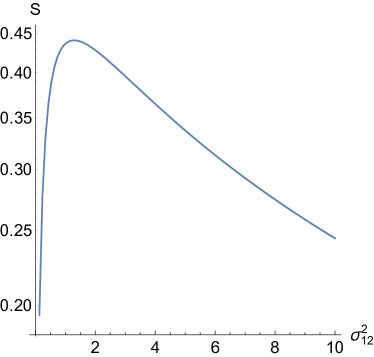
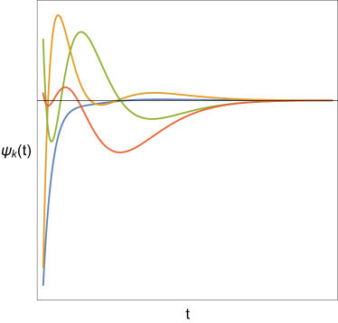
Figure 3: (a) Entropy vs. cross-correlation magnitude $\sigma_{12}$ in the case of slow-modulation (Homogenous broadening limit). (b) Schmidt modes for maximally entangled state ($\sigma_{12}^{2}=1.33$).

An interesting case arises when

$${\cal K}^{(2)}=a\delta(t-t^{\prime}).$$

Since one can write the delta-function as a resolution of the identity in terms of orthogonal polynomials $O_{n}(x)$, Lamata and León (2005)

$$\delta(t-t^{\prime})=\lim_{N\to\infty}\sum_{k=0}^{N}O_{k}(t)O_{k}(t^{\prime}),$$ (55)

its normalized Schmidt coefficients are all equal to $1/\sqrt{N}$. This gives rise to the case of maximal entanglement entropy since

$$S=-\lim_{N\to\infty}\sum_{k=0}^{N}\frac{1}{N}\log(1/N)\to\infty.$$ (56)

IV Discussion

We have presented here a model for the generation of entanglement entropy for a biphoton Fock state interacting with a material sample. We assume that the two-photon scattering matrix can be decomposed into a series of single photon/photon interactions mediated by coupling to a medium with coupling strength $\xi$. In the limit that the scattering produces a random phase shift, the entanglement collapses and the outgoing state is a single Fock state. However, in the case of Gaussian noise, the entanglement entropy increases with increasing coupling producing squeezed states. We also present a microscopic model for the photon-photon coupling for the case of two photons passing through an optical cavity. Here, we again show that in the limit of fast fluctuations and motional narrowing, the entanglement entropy vanishes where as in the case of slow modulation (homogeneous broadening) the entanglement entropy reaches a maximum value depending upon the magnitude of the fluctuations. Our analysis shows that two-photon entanglement scattering provides a direct and sensitive probe of correlated fluctuations within the sample system.

Author Contributions

ERB, CS, and AP conceived and developed the core ideas. ERB, HL, and AP developed and implemented the formalism. All authors participated in the discussion of the methods and results. All authors participated in the drafting and final editing of this manuscript.

Competing financial interests

The authors declare no competing financial interests.

Appendix A Photon mode scattering via cavity polariton fluctuations

In this Appendix adopted stochastic Hamiltonian (32) is derived based on a simple model describing light scattering by the fluctuations of delocalized polariton modes confined in an optical cavity. For this situation, the photon Hamiltonian can be represented as a sum of two components

$$\hat{H}_{\text{ph}}=\hat{H}_{\text{o}}+\hat{H}_{\text{s}}.$$ (57)

Assuming that biphoton wavepacket is spatially confined within a cross section of area $A$ and propagates in the $z$-direction, the interaction free photon Hamiltonian in the continues mode representation readsLoudon (2000b)

$$\hat{H}_{\text{o}}=\sum\limits_{j=1,2}\int d\omega_{j}\omega_{j}\hat{b}_{\omega_{j}}^{\dagger}\hat{b}_{\omega_{j}}.$$ (58)

with index $j$ distinguishing the modes.

The photon scattering illustrated in Fig. 1 is described by the interaction Hamiltonian

$$\hat{H}_{\text{s}}=-\iint\limits_{A}dxdy\int\limits_{-L/2}^{L/2}dz\sum\limits_{j=1,2}\hat{\alpha}_{jj}(\bm{r})\hat{E}_{j}(z)^{2},$$ (59)

where the integration $dS$ over the photon wave packet cross section ($x,y$-plane) is partitioned from the spatial integral in the propagation direction $z$. The cavity cross-section is assumed to be larger than $A$ and the length is denoted by $L$. The electric field operator for the photon modes of interest represented in terms of the mode creation and annihilation operators readsLoudon (2000b)

$$\hat{E}_{j}(z) = i\int d\omega_{j}\sqrt{\frac{\hbar\omega_{j}}{4\pi\varepsilon_{o}cA}}\left(b_{\omega_{j}}e^{i\omega_{j}z/c}-b_{\omega_{j}}^{\dagger}e^{-i\omega_{j}z/c}\right),\;\;\;\;\;\;\;$$ (60)

where $c$ is speed of light and $\varepsilon_{o}$ is the vacuum permittivity.

Evaluation of the integrals in the scattering Hamiltonian (59) requires a model for the sample polarizability operator $\hat{\alpha}(\bm{r})$. Let us consider delocalized cavity polariton modes which we described by operator

$$\hat{\zeta}_{\bm{k}_{l}}=\bar{\zeta}_{\bm{k}_{l}}+\delta\hat{\zeta}_{\bm{k}_{l}}(t).$$ (61)

where $\bm{k}_{l}$ denotes $s$-th polariton mode wave vector. $\bar{\zeta}_{\bm{k}_{l}}$ is a cavity polariton steady state prepared by a resonant external pumping and $\delta\hat{\zeta}_{\bm{k}_{l}}(t)$ is time-dependent mode fluctuation operator. Accordingly, the polarizability can be expanded up to the first order in the fluctuations

$$\hat{\alpha}_{jj} = \alpha_{jj}(\bar{\zeta}_{\bm{k}_{l}})+\sum\limits_{l}\sum\limits_{\bm{k}_{l}}\frac{\partial\alpha_{jj}(\bar{\zeta}_{\bm{k}_{l}})}{\partial\bar{\zeta}_{\bm{k}_{l}}}\delta\hat{\zeta}_{\bm{k}_{l}}(t).$$ (62)

For further analysis the fluctuation operator is expanded in terms of polariton spatial Fourier components

$$\delta\hat{\zeta}_{\bm{k}_{l}}(t)=\delta\hat{\zeta}^{+}_{\bm{k}_{l}}(t)e^{i\bm{k}_{l}\bm{r}}+\delta\hat{\zeta}_{\bm{k}_{l}}^{-}(t)e^{-i\bm{k}_{l}\bm{r}}.$$ (63)

Making substitution of the second term in Eq. (62) along with Eq. (63) into the scattering Hamiltonian (59) where the electric field is introduced by Eq. (60), performing integration over the cavity volume, and further neglecting the terms describing simultaneous two-photon creation and annihilation processes, we obtain

$$\hat{H}_{\text{s}} = -\hbar\sum_{l}\sum\limits_{k_{l}}\sum\limits_{j=1,2}\int d\omega_{j}\kappa_{k_{l}}(\omega^{\prime})$$

$$\times \left(\hat{b}_{\omega_{j}+ck_{l}}^{\dagger}\hat{b}_{\omega_{j}}\delta\hat{\zeta}^{+}_{k_{l}}+\hat{b}_{\omega_{j}}^{\dagger}\hat{b}_{\omega_{j}+ck_{l}}\delta\hat{\zeta}^{-}_{k_{l}}\right),$$

with the coupling parameter

$$\kappa_{k_{l}}(\omega_{j}) = \frac{1}{\varepsilon_{o}L}\left.\frac{\partial\alpha_{jj}(\bar{\zeta}_{\bm{k}_{l}})}{\partial\bar{\zeta}_{\bm{k}_{l}}}\right|_{\bm{k}^{\bot}_{l}=0}\left[(\omega_{j}-ck_{l})\omega_{j}\right]^{1/2}.$$ (65)

Since the photons propagate in $z$-direction, the total momentum conservation requires that the scattered photon momentum changes for the amount of $k_{j}$ which is the $z$-component of the total momentum $\bm{k}_{j}$. Accordingly, the transverse ($xy$-plane) component of the momentum $\bm{k}_{j}^{\bot}$ does not change resulting in the photon coupling to the $\Gamma$-point of transverse polariton band as indicated above by setting $\bm{k}^{\bot}_{j}=0$.

Taking into account that polariton modes have continuous dispersion relations $k_{l}=k(\omega_{l})$ , we replace sum over $k_{l}$ in Eq. (A) by the integral over $d\omega_{l}$. This results in

$$\hat{H}_{\text{s}} = -\hbar\sum\limits_{j=1,2}\sum_{l}\iint d\omega_{j}d\omega_{l}~{}\kappa(\omega_{j}\omega_{l})$$

$$\times \left(\hat{b}_{\omega_{j}+\omega_{l}}^{\dagger}\hat{b}_{\omega_{j}}\delta\hat{\zeta}^{+}_{\omega_{l}}+\hat{b}_{\omega_{j}}^{\dagger}\hat{b}_{\omega_{j}+\omega_{l}}\delta\hat{\zeta}^{-}_{\omega_{l}}\right),$$

with the coupling parameter

$$\kappa(\omega_{j}\omega_{l}) = \frac{1}{2\pi\varepsilon_{o}}\left.\frac{\partial\alpha_{j}j(\bar{\zeta}_{\bm{k}(\omega_{l})})}{\partial\bar{\zeta}_{\bm{k}(\omega_{l})}}\right|_{\bm{k}^{\bot}(\omega_{l})=0}$$

$$\times \frac{\partial k(\omega_{l})}{\partial\omega_{l}}\left[(\omega_{j}-\omega_{l})\omega_{j}\right]^{1/2}.$$

The scattering Hamiltonian (A) can be further simplified, provided the interaction occurs near the bottom of polariton modes, i.e. $\omega_{l}\sim 0$. In this case one can set

$$\left.\frac{\partial\alpha_{jj}(\bar{\zeta}_{\bm{k}(\omega_{l})})}{\partial\bar{\zeta}_{\bm{k}(\omega_{l})}}\right|_{\bm{k}^{\bot}(\omega_{l})=0}=\bar{\alpha}_{jj}\delta(\omega_{l}).$$ (68)

with $\bar{\alpha}_{jj}$ being a coupling constant. Substitution of Eq. (A) with Eq. (dalpha-loc) into Eq. (A) recasts the latter to the form of stochastic Hamiltonian (32) with the frequency fluctuation operator defined as

$$\delta\omega_{j}=\frac{\bar{\alpha}_{jj}\omega_{j}}{2\pi\varepsilon_{o}}\sum_{l}\frac{\partial k(\omega_{l})}{\partial\omega_{l}}\delta\hat{\zeta}_{l}.$$ (69)

where a shorthand notation $\delta\hat{\zeta}_{l}=\delta\hat{\zeta}_{\omega_{l}=0}$ is used.

Appendix B Evaluation of second cumulants for Gaussian stochastic process

In this Appendix, we derive explicit form of the single-mode and cross-mode cumulant functions using the correlation functions for stochastic Gaussian processes given in Eqs. (45) and (46), respectively.

Evaluation of time ordered integral in Eq. (43) with the correlation function given by Eq. (45) results in a well known form of the second cumulantKubo (2007)

$$g_{j}(t-t^{\prime}) = (\sigma_{j}\bar{\tau}_{j})^{2}$$

$$\times \left\{(t-t^{\prime})/\bar{\tau}_{j}+e^{-(t-t^{\prime})/\bar{\tau}_{j}}+1\right\}.\;\;\;\;\;\;$$

In the case of inhomogeneous broadening $\sigma\bar{\tau}_{j}\ll 1$ one gets

$$g_{j}(t-t^{\prime}) = \gamma_{j}(t-t^{\prime}),$$ (71)

with $\gamma_{j}=\sigma^{2}\bar{\tau}_{j}$. In the case of homogeneous broadening $\sigma\bar{\tau}_{j}\gg 1$ one gets

$$g_{j}(t-t^{\prime}) = \sigma_{j}^{2}(t-t^{\prime})^{2}.$$ (72)

Evaluation of the integrals in Eq. (44) with the cross-correlation function in Eq. (46) is not so straight forward and one needs to take into account various ordering of $t_{1}^{\prime}$, $t_{1}$, $t_{2}^{\prime}$ and $t_{2}$:

with three more corresponding to swapping index $1$ and $2$ (but not the primes).

$$g^{+}_{12}(t_{1}t_{1}^{\prime}t_{2}t_{2}^{\prime}) = (\sigma_{12}\bar{\tau}_{12})^{2}\left\{\right.$$

$$\left.e^{-(t_{1}-t_{2})/\bar{\tau}_{12}}-e^{-(t_{1}-t_{2}^{\prime})/\bar{\tau}_{12}}\right.$$

$$+ \left.e^{-(t_{1}^{\prime}-t_{2})/\bar{\tau}_{12}}-e^{-(t_{1}^{\prime}-t_{2}^{\prime})/\bar{\tau}_{12}}\right\},\;\;\;\;$$

$$g^{+}_{12}(t_{1}t_{2}t_{1}^{\prime}t_{2}^{\prime}) = (\sigma_{12}\bar{\tau}_{12})^{2}\left\{2(t_{2}-t_{1}^{\prime})/\bar{\tau}_{12}\right.$$

$$- \left.e^{-(t_{1}-t_{2})/\bar{\tau}_{12}}+e^{-(t_{1}-t_{2}^{\prime})/\bar{\tau}_{12}}\right.$$

$$- \left.e^{-(t_{1}^{\prime}-t_{2}^{\prime})/\bar{\tau}_{12}}+e^{-(t_{2}-t_{1}^{\prime})/\bar{\tau}_{12}}\right\},\;\;\;\;$$

$$g_{12}^{+}(t_{1}t_{2}t_{2}^{\prime}t_{1}^{\prime}) = (\sigma_{12}\bar{\tau}_{12})^{2}\left\{2(t_{2}-t_{2}^{\prime})/\bar{\tau}_{12}\right.$$

$$- \left.e^{-(t_{2}^{\prime}-t_{1}^{\prime})/\bar{\tau}_{12}}+e^{-(t_{2}-t_{1}^{\prime})/\bar{\tau}_{12}}\right.$$

$$- \left.e^{-(t_{1}-t_{2})/\bar{\tau}_{12}}+e^{-(t_{1}-t_{2}^{\prime})/\bar{\tau}_{12}}\right\},\;\;\;\;$$

and three more

$$g^{+}_{12}(t_{2}t_{1}t_{1}^{\prime}t_{2}^{\prime}) = (\sigma_{12}\bar{\tau}_{12})^{2}\left\{2(t_{1}-t_{1}^{\prime})/\bar{\tau}_{12}\right.$$

$$- \left.e^{-(t_{1}^{\prime}-t_{2}^{\prime})/\bar{\tau}_{12}}+e^{-(t_{1}-t_{2}^{\prime})/\bar{\tau}_{12}}\right.$$

$$- \left.e^{-(t_{2}-t_{1})/\bar{\tau}_{12}}+e^{-(t_{2}-t_{1}^{\prime})/\bar{\tau}_{12}}\right\},\;\;\;\;$$

$$g^{+}_{12}(t_{2}t_{1}t_{2}^{\prime}t_{1}^{\prime}) = (\sigma_{12}\bar{\tau}_{12})^{2}\left\{2(t_{1}-t_{2}^{\prime})/\bar{\tau}_{12}\right.$$

$$- \left.e^{-(t_{2}-t_{1})/\bar{\tau}_{12}}+e^{-(t_{2}-t_{1}^{\prime})/\bar{\tau}_{12}}\right.$$

$$- \left.e^{-(t_{2}^{\prime}-t_{1}^{\prime})/\bar{\tau}_{12}}+e^{-(t_{1}-t_{2}^{\prime})/\bar{\tau}_{12}}\right\},\;\;\;\;$$

$$g^{+}_{12}(t_{2}t_{2}^{\prime}t_{1}t_{1}^{\prime}) = (\sigma_{12}\bar{\tau}_{12})^{2}\left\{\right.$$

$$\left.e^{-(t_{2}-t_{1})/\bar{\tau}_{12}}-e^{-(t_{2}-t_{1}^{\prime})/\bar{\tau}_{12}}\right.$$

$$+ \left.e^{-(t_{2}^{\prime}-t_{1})/\bar{\tau}_{12}}-e^{-(t_{2}^{\prime}-t_{1}^{\prime})/\bar{\tau}_{12}}\right\},\;\;\;\;$$

with time indices 1 and 2 swapped. Note, our notation is such that in $g_{12}^{+}(t_{a}t_{b}t_{c}t_{d})$, $t_{a}>t_{b}>t_{c}>t_{d}$.

In the case of inhomogeneous broadening $\sigma_{12}\bar{\tau}_{12}\ll 1$, $g^{+}_{12}(t_{1}t_{1}^{\prime}t_{2}t_{2}^{\prime})=0$, $g^{+}_{12}(t_{2}t_{2}^{\prime}t_{1}t_{1}^{\prime})=0$, and the rest of time-ordered cumulants simplify to the form

$$g^{+}_{12}(t_{1}t_{2}t_{1}^{\prime}t_{2}^{\prime}) = \gamma_{12}(t_{2}-t_{1}^{\prime}),$$ (79)

$$g_{12}^{+}(t_{1}t_{2}t_{2}^{\prime}t_{1}^{\prime}) = \gamma_{12}(t_{2}-t_{2}^{\prime}),$$ (80)

$$g^{+}_{12}(t_{2}t_{1}t_{2}^{\prime}t_{1}^{\prime}) = \gamma_{12}(t_{1}-t_{2}^{\prime}),$$ (81)

$$g_{12}^{+}(t_{2}t_{1}t_{1}^{\prime}t_{2}^{\prime}) = \gamma_{12}(t_{1}-t_{1}^{\prime}),$$ (82)

with $\gamma_{12}=\sigma_{12}^{2}\bar{\tau}_{12}$.

In the case of homogeneous broadening $\sigma_{12}\bar{\tau}_{12}\gg 1$, Eqs. (B)-(B) simplify to the following expression

$$g_{12}(t-t^{\prime}) = \sigma_{12}^{2}(t_{1}-t_{1}^{\prime})(t_{2}-t_{2}^{\prime}),$$ (83)

which holds for all initial time permutations used in Eqs. (B)-(B) .

References

• Tyndall (1869a) J. Tyndall, Phil. Mag. 38, 156 (1869a).
• Tyndall (1863) J. Tyndall, Phil. Mag. 25, 200 (1863).
• Tyndall (1869b) J. Tyndall, Phil. Mag. 37, 384 (1869b).
• Lord Rayleigh (1871a) (Strutt, J. W.) Lord Rayleigh (Strutt, J. W.), Phil. Mag. 41, 107 (1871a).
• Lord Rayleigh (1871b) (Strutt, J. W.) Lord Rayleigh (Strutt, J. W.), Phil. Mag. 41, 274 (1871b).
• Lord Rayleigh (1871c) (Strutt, J. W.) Lord Rayleigh (Strutt, J. W.), Phil. Mag. 41, 447 (1871c).
• Lord Rayleigh (1899) (Strutt, J. W.) Lord Rayleigh (Strutt, J. W.), Phil. Mag. 47, 375 (1899).
• Berne and Pecora (1976) B. Berne and R. Pecora, Dynamic Llght Scattering, wlth Appllcatlons to Chemlstry, Biology, and Physics (John Wiley and Sons, New York, 1976).
• Ladd et al. (2010) T. D. Ladd, F. Jelezko, R. Laflamme, Y. Nakamura, C. Monroe,  and J. L. O’Brien, Nature 464, 45 (2010).
• Lemos et al. (2014) G. B. Lemos, V. Borish, G. D. Cole, S. Ramelow, R. Lapkiewicz,  and A. Zeilinger, Nature 512, 409 (2014).
• Gisin et al. (2002) N. Gisin, G. Ribordy, W. Tittel,  and H. Zbinden, Rev. Mod. Phys. 74, 145 (2002).
• Sewell (2017) R. Sewell, Physics 10, 38 (2017).
• Zou, Wang, and Mandel (1991) X. Y. Zou, L. J. Wang,  and L. Mandel, Physical review letters 67, 318 (1991).
• Roslyak, Marx, and Mukamel (2009) O. Roslyak, C. A. Marx,  and S. Mukamel, Phys. Rev. A 79, 033832 (2009).
• Schlawin et al. (2013) F. Schlawin, K. E. Dorfman, B. P. Fingerhut, S. Mukamel,  and S. Mukamel, Nature Communications 4, 1782 (2013).
• Li et al. (2018) H. Li, A. Piryatinski, J. Jerke, A. R. S. Kandada, C. Silva,  and E. R. Bittner, Quantum Sci. Technol. 3, 015003 (2018).
• Loudon (2000a) R. Loudon, The quantum theory of light (Oxford University Press, New York, 2000).
• Gardiner and Savage (1984) C. Gardiner and C. Savage, Optics Comm. 50, 173 (1984).
• Collett and Gardiner (1984) M. J. Collett and C. W. Gardiner, Phys. Rev. A 30, 1386 (1984).
• Gardiner and Collett (1985) C. W. Gardiner and M. J. Collett, Phys. Rev. A 31, 3761 (1985).
• Kubo (2007) R. Kubo, “A stochastic theory of line shape,” in Advances in Chemical Physics, Advances in Chemical Physics, edited by K. E. Shuler (Wiley-Blackwell, 2007) pp. 101–127, https://onlinelibrary.wiley.com/doi/pdf/10.1002/9780470143605.ch6 .
• Mukamel (1995) S. Mukamel, Principles of Nonlinear Optics and Spectroscopy (Oxford University Press, 1995).
• Lamata and León (2005) L. Lamata and J. León, Journal of Optics B: Quantum and Semiclassical Optics 7, 224 (2005).
• Note (1) We suggest this state be termed the “Goldilocks State”.
• Loudon (2000b) R. Loudon, Quantum Theory of Light (Oxford Science Publications, 2000).