Quadrature Histograms in Maximum Likelihood Quantum State Tomography

Abstract

Quantum state tomography aims to determine the quantum state of a system from measured data and is an essential tool for quantum information science. When dealing with continuous variable quantum states of light, tomography is often done by measuring the field amplitudes at different optical phases using homodyne detection. The quadrature-phase homodyne measurement outputs a continuous variable, so to reduce the computational cost of tomography, researchers often discretize the measurements. We show that this can be done without significantly degrading the fidelity between the estimated state and the true state. This paper studies different strategies for determining the histogram bin widths. We show that computation time can be significantly reduced with little loss in the fidelity of the estimated state when the measurement operators corresponding to each histogram bin are integrated over the bin width.

I Introduction

Quantum information science and engineering have advanced to the point where rudimentary quantum computers are available in the laboratory and commercially Kandala et al. (2014); Linke et al. (2017); Monz et al. (2017); Denchev et al. (2016). However, further advancing quantum technologies requires improvements in the fidelities of basic operations. Consequently, more precise and efficient reconstruction and diagnostic tools for estimation of quantum states Vogel and Risken (1989); Smithey et al. (1993); Dunn et al. (1995); Banaszek et al. (1999, 2000); White et al. (2002); Ourjoumtsev et al. (2007); Neergaard-Nielsen et al. (2006), processes Chuang and Nielsen (1997); Poyatos et al. (1997); Altepeter et al. (2003); D’Ariano and Maccone (1998); Nielsen et al. (1998); Mitchell et al. (2003); O’Brien et al. (2004); Kupchak et al. (2015), and measurements Luis and Sanchez-Soto (1999); Fiurasek (2001); D’Ariano et al. (2004); Lundeen et al. (2009) are essential. Quantum tomographic techniques for optical quantum states of light have become standard tools because quantum light sources are essential for implementations of continuous-variable (CV) quantum computation and communication Lloyd and Braunstein (1999); Gottesman et al. (2001); Bartlett et al. (2002); Jeong and Kim (2002); Ralph et al. (2003). These source are also extensively exploited in quantum cryptography Ralph (1999); Hillery (2000); Silberhorn et al. (2002); Pirandola et al. (2008); Luiz and Rigolin (2017), quantum metrology Eberle et al. (2004); Demkowicz-Dobrzański et al. (2013), state teleportation Vaidman (1994); Braunstein and Kimble (1998); He et al. (2015), dense coding Braunstein and Kimble (2000); Lee et al. (2014) and cloning Cerf and Iblisdir (2000); Braunstein et al. (2001).

In the quantum state tomography studied here, one performs a measurement on each member of a collection of quantum systems, prepared in the same unknown state. Each system is measured in a basis chosen from a complete set of measurements. The goal is to estimate the unknown state from the measurements results. This estimation can be done by different methods, but we study Maximum Likelihood Estimation (MLE), which finds among all possible states, the one that maximizes the likelihood function. The likelihood function computes for any state the probability, according to that state, of obtaining the observed data.

Quantum homodyne tomography is one of the most popular optical tomography techniques available Lvovsky (2004). It rapidly became a versatile tool and has been applied in many different quantum optics experimental settings since it was proposed by Vogel and Risken in 1989 Vogel and Risken (1989) and first implemented by Smithey et al. in 1993 Smithey et al. (1993). This technique permits one to characterize an optical quantum state by analyzing multiple phase-sensitive measurements of the field quadratures.

A homodyne measurement generates a continuous value. It is a popular practice to discretize the measurement result, because this can considerably reduce the size of the data and expedite the reconstruction calculation. However the discretization necessarily loses information contained in the original measurements. How should we choose a discretization strategy such that the bins are not too small nor too large? Larger bins will reduce calculation time and memory, but smaller bins will provide a better representation of the underlying distribution.

In this paper, we use numerical experiments to simulate optical homodyne tomography and perform maximum likelihood tomography on the data with and without discretization. When choosing a quadrature bin width, we use and compare two different strategies: Scott’s rule Scott (2010) and Leonhardt’s formula Leonhardt et al. (1996). The paper is divided as follow: we begin by reviewing maximum likelihood in homodyne tomography in Section II. Then, in Section III, we describe our numerical experiments. Next, we discuss the estimation of the mean photon number from the quadrature measurements in Section IV. In Section V we present our results, and we make our concluding remarks in Section VI.

II Maximum likelihood in homodyne tomography

Let us consider $N$ quantum systems, each prepared in an optical state described by a density matrix $\rho_{\text{true}}$. In each experimental trial $i$, we measure the field quadrature of one of the systems at some phase $\theta_{i}$ of a local oscillator, i.e. a reference system prepared in a high amplitude coherent state. Each measurement is associated with an observable $\hat{X}_{\theta_{i}}=\hat{X}\cos\theta_{i}+\hat{P}\sin\theta_{i}$, where $\hat{X}$ and $\hat{P}$ are analogous to mechanical position and momentum operators, respectively. For a given phase $\theta_{i}$, we measure a quadrature value $x_{i}$, resulting in the data $\{(\theta_{i},x_{i})|i=1,\ldots,N\}$.

The outcome of the $i$-th measurement is associated with a positive-operator-valued measure (POVM) element $\Pi(x_{i}|\theta_{i})=\Pi_{i}$. Given the data, the likelihood of a candidate density matrix $\rho$ is

$$\mathcal{L}(\rho)=\prod_{i=1}^{N}\mathrm{Tr}(\Pi_{i}\rho),$$ (1)

where $\mathrm{Tr}(\rho\Pi_{i})$ is the probability density, when measuring with phase $\theta_{i}$, to obtain outcome $x_{i}$, according to the candidate density matrix $\rho$.

MLE searches for the density matrix that maximizes the likelihood in Eq. (1). It usually is more convenient to maximize the logarithm of the likelihood (the “log-likelihood”):

$$L(\rho)=\ln\mathcal{L}(\rho)=\sum_{i=1}^{N}\ln[\mathrm{Tr}(\Pi_{i}\rho)],$$ (2)

which is maximized by the same density matrix as the likelihood. The MLE is essentially a function optimization problem, and since the log-likelihood function is concave, approximate convergence to a unique solution will be achieved by most iterative optimization methods.

In our numerical simulations, we use an algorithm for likelihood maximization that begins with iterations of the $R\rho R$ algorithm Řeháček et al. (2007) followed by iterations of a regularized gradient ascent (RGA) algorithm. We switch from one algorithm to another because a slow-down is observed in the $R\rho R$ algorithm after about $(t+1)^{2}/4$ iterations, where $t+1$ is the Hilbert space dimension. In the RGA, $\rho^{(k+1)}$ is parametrized as

$$\rho^{(k+1)}=\frac{\left(\sqrt{\rho^{(k)}}+A\right)\left(\sqrt{\rho^{(k)}}+A^{\dagger}\right)}{\mathrm{Tr}\left[\left(\sqrt{\rho^{(k)}}+A\right)\left(\sqrt{\rho^{(k)}}+A^{\dagger}\right)\right]},$$ (3)

where $\rho^{(k)}$ is the density matrix found by the previous iteration, and $A$ may be any complex matrix of the same dimensions as $\rho$. Eq. (3) ensures that $\rho^{(k+1)}$ is a density matrix for any $A$. We then use sequential quadratic programming optimization strategy Nocedal and Wright (2006) in which $A$ is chosen to maximize the quadratic approximation of the log-likelihood subject to $\text{Tr}(AA^{\dagger})\leq u$, where $u$ is a positive number adjusted by the algorithm to guarantee that the log-likelihood increases with each iteration. To halt the iterations, we use the stopping criterion of Glancy et al. (2012), $L(\rho_{\text{ML}})-L(\rho^{(k)})\leq 0.2$, where $L(\rho_{\text{ML}})$ is the maximum of the log-likelihood, which ensures convergence to a state whose log-likelihood is very close to the maximum likelihood.

III Methods for Numerical experiments

Our numerical experiments simulate single mode optical homodyne measurements of three types of states: (1) superpositions of coherent states of opposite phase $|-\alpha\rangle+|\alpha\rangle$ (called “cat states”), (2) squeezed vacuum states and (3) Fock states. Each state is represented by a density matrix $\rho_{\mathrm{true}}$ represented in the photon number basis, truncated at $t$ photons. To better simulate realistic experiments, these pure states are subject to a 0.05 photon loss by passing through a medium with transmissivity of 0.95 before measurement.

In order to calculate the probability to obtain homodyne measurement outcome $x$, when measuring state $\rho_{\mathrm{true}}$ with phase $\theta$, we represent all states and measurements in the photon number basis of a Hilbert space truncated at $t$ photons. If $|x\rangle$ is the x-quadrature eigenstate with eigenvalue $x$, and $U(\theta)$ is the phase evolution unitary operator, then for an ideal homodyne measurement, we have $\Pi(x|\theta)=U(\theta)^{\dagger}|x\rangle\langle x|U(\theta)$. To include photon detector inefficiency, we replace the projector with $\Pi(x|\theta)=\sum_{i=1}^{n}E_{i}(\eta)^{\dagger}U(\theta)^{\dagger}|x\rangle\langle x|U(\theta)E_{i}(\eta)$, where $\eta$ is the detection efficiency and $E_{i}(\eta)$ are the associated Kraus operators Lvovsky (2004). Typical state-of-the-art homodyne detection systems have efficiency $\eta\sim 0.9$, so we use this value in our simulations. Using this strategy, we are able to correct for the detector inefficiency as we estimate the state. We use rejection sampling from the distribution given by $P(x|\theta)$ to produce random samples of homodyne measurement results Jr. and Gentle (1980).

To choose the phases at which the homodyne measurements are performed, we divide the upper-half-circle evenly among $m$ phases between 0 and $\pi$ and measure $N/m$ times at each phase, where $N$ is the total number of measurements. In all simulations, we use $m=20$ and $N=20,000$. To secure a single maximum of the likelihood function, we need an informationally complete set of measurement operators, which can be obtained if we use $t+1$ different phases to reconstruct a state that contains at most $t$ photons Leonhardt (1997).

To quantify the similarity of the reconstructed state $\rho$ to the true state $\rho_{\text{true}}$ we use the fidelity

$$F=\mathrm{Tr}\sqrt{\rho^{1/2}\,\rho_{\text{true}}\,\rho^{1/2}}.$$ (4)

We report fidelities for four different situations: (i) the state is reconstructed using the continuous values of homodyne measurement results, that is without discretization; (ii) the state is reconstructed with chosen bin widths (iii) the state is reconstructed with bin widths given by Scott’s rule Scott (2010); and (iv) the state is reconstructed with bin widths suggested by Leonhardt in Leonhardt (1997). We only consider histograms with contiguous bins of equal width.

In 1979 Scott derived a formula recommending a bin width for discretizing data sampled from a probability density function $f$ for a single random variable $x$. The recommended bin width is

$$h^{\star}=\left[\frac{6}{s\int_{-\infty}^{\infty}f^{\prime}(x)^{2}dx}\right]^{1/3},$$ (5)

where the first and second derivatives of $f$ must be continuous and bounded and $s$ is the sample size. Because one does not know $f$ in an experiment we assume a normal distribution. For a normal $f$ we have

$$\int_{-\infty}^{\infty}f^{\prime}(x)^{2}dx=\frac{1}{4\sqrt{\pi}\sigma^{3}},$$ (6)

where $\sigma$ is the distribution’s standard deviation. Combining Eqs. (5) and (6), we obtain the recommended bin width for a normal distribution:

$$h=3.5\,\sigma\,s^{-1/3}.$$ (7)

This formula is known as Scott’s rule, and is optimal for estimating $f$ (minimizing total mean-squared error) at each phase if the data is normally distributed. In our simulations we compute a bin size separately for each phase’s quadrature measurements, and we use the unbiased sample standard deviation in place of $\sigma$.

Although Scott’s rule is optimal for each phase, it may not be optimal for homodyne tomography because we are estimating the density matrix rather than each phase’s quadrature distribution individually. Also many interesting optical states do not have normal quadrature distributions, for example our cat states. In fact, one might expect that the bin width should be related to the number of photons in a quantum state because higher photon number states have more narrow features in their quadrature distributions, which should not be washed-out by the discretization.

Leonhardt states that if we desire to reconstruct a density matrix of a state with $n$ photons, we need a bin width narrower than $q_{n}/2$, where $q_{n}$ is given by

$$q_{n}=\frac{\pi}{\sqrt{2n+1}}.$$ (8)

This result was obtained from a semiclassical approximation for the amplitude pattern functions in quantum state sampling Leonhardt et al. (1996). Leonhardt recommends using the maximum photon number in Eq. (8), however many states have no maximum photon number, and whether a state has a maximum photon number is not possible to learn with certainty from tomography. Instead, we have tested using the photon number $t$ at which the reconstruction Hilbert space is truncated and an estimate of the mean photon number $\overline{\langle\hat{n}\rangle}$ in Eq. (8). The truncation $t$ must be chosen in advance to be large enough that the probability that $\rho_{\text{true}}$ contains more than $t$ photons is very small. We estimate the mean photon number from the quadrature measurements as described in the next section.

IV Estimating mean photon number

In order to use Leonhardt’s advice for choosing the histogram bin width, we need to estimate the mean number $\langle\hat{n}\rangle$ of photons in the measured state from the phase-quadrature data set. We use the estimator given in Refs. Raymer and Beck (2004); Munroe (1996). To obtain this estimator, we first compute the mean value of $(\hat{X}_{\theta})^{2}$, averaged over $\theta$, treating $\theta$ as if it is random and uniformly distributed between $0$ and $\pi$.

$$\langle(\hat{X}_{\theta})^{2}\rangle=\langle\hat{X}^{2}\cos^{2}\theta+(\hat{X}\hat{P}+\hat{P}\hat{X})\cos\theta\sin\theta+\hat{P}^{2}\sin^{2}\theta\rangle$$ (9)

The phase $\theta$ is independent of $\hat{X}$ and $\hat{P}$, so we can compute the expectation over $\theta$ as

$$\langle(\hat{X}_{\theta})^{2}\rangle =\Big{\langle}\int_{0}^{\pi}(\hat{X}^{2}\cos^{2}\theta+(\hat{X}\hat{P}+\hat{P}\hat{X})\cos\theta\sin\theta$$

$$\qquad\qquad+\hat{P}^{2}\sin^{2}\theta)\mathrm{Prob}(\theta)\mathrm{d}\theta\Big{\rangle}$$ (10)

$$\langle(\hat{X}_{\theta})^{2}\rangle =\Big{\langle}\int_{0}^{\pi}(\hat{X}^{2}\cos^{2}\theta+(\hat{X}\hat{P}+\hat{P}\hat{X})\cos\theta\sin\theta$$

$$\qquad\qquad+\hat{P}^{2}\sin^{2}\theta)\frac{1}{\pi}\mathrm{d}\theta\Big{\rangle}$$ (11)

$$=\frac{1}{2}\left\langle\hat{X}^{2}+\hat{P}^{2}\right\rangle.$$ (12)

Because the photon number operator is

$$\hat{n}=\frac{1}{2}\left(\hat{X}^{2}+\hat{P}^{2}-1\right),$$ (13)

we obtain

$$\langle\hat{n}\rangle=\langle\hat{X}_{\theta}^{2}\rangle-\frac{1}{2}.$$ (14)

We estimate $\langle\hat{n}\rangle$ by computing the sample mean of all quadrature measurements Raymer and Beck (2004); Munroe (1996):

$$\overline{\langle\hat{n}\rangle}=\frac{1}{N}\sum_{i=1}^{N}x_{i}^{2}-\frac{1}{2},$$ (15)

where the bar above $\overline{\langle\hat{n}\rangle}$ distinguishes the true mean photon number from our estimate of the mean photon number. Note that when $\theta$ is uniformly distributed over $[0,\pi)$, the individual values of $\theta$ are not needed to compute $\overline{\langle\hat{n}\rangle}$.

V Results

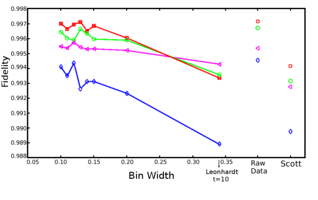
Figure 1: Fidelities between estimated states and true states as functions of the bin width for a cat state with amplitude $\alpha=1$ and photon loss of 0.05. The Hilbert space is truncated at $t=10$ photons. Each set of points with the same color and marker shape corresponds to a different data set. The mean bin width for Scott method is $0.35$.

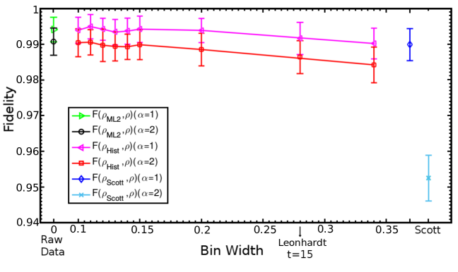
Figure 2: Average fidelity as a function of the bin width for cat states with amplitudes $\alpha=1$ and $\alpha=2$. The Hilbert space is truncated at $t=15$ photons. The mean bin widths for Scott’s method are $0.35$ ($\alpha=1$ cat state) and $0.64$ ($\alpha=2$ cat state).

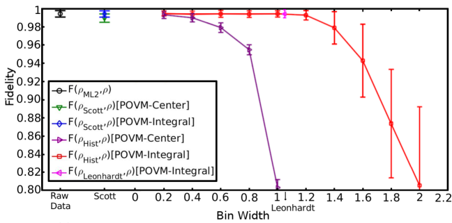
Figure 3: Average fidelity as a function of the bin width for a cat state with amplitude $\alpha=1$. The Hilbert space is truncated at $t=10$ photons. For this state, $\langle n\rangle=0.6093$, and $\overline{\langle\hat{n}\rangle}=0.6109$, giving a bin width by Leonhardt’s formula of $1.05$. The mean bin width for Scott’s method is $0.35$.

To study the performance of various discretization strategies, we compute fidelities between the true state and the states estimated with the different strategies. Below $\rho_{\mathrm{ML2}}$ represents the state estimated without discretization, $\rho_{\mathrm{Hist}}$ is estimated with histogram bins of specified width chosen arbitrarily, $\rho_{\mathrm{Scott}}$ is estimated with bin widths chosen according to Scott’s rule, and $\rho_{\mathrm{Leonhardt}}$ is estimated with Leonhardt’s bin widths. To make the graphs below, for each choice of parameters, we simulate 100 tomography experiments, making 100 density matrix estimates. The graphs show the arithmetic mean of the 100 fidelities of the reconstructed states. The half width of the error bars are the sample standard deviations of the 100 fidelities.

Our first results are shown in Fig. 1. The state considered is a cat state with $\alpha=1$, where $\alpha$ is the amplitude of the coherent state in the superposition. The state is reconstructed in a Hilbert space truncated at $t=10$ photons. (The probability that the $\alpha=1$ state has more than 10 photons is $3.8\times 10^{-10}$.) Scott’s method finds a different optimal bin width for each phase considered, so we report the mean bin width averaged over the 20 phases in these cases. Here the mean bin width for Scott’s method is $0.35$. When choosing a bin width, we use values up to $0.34$, the width we obtain when we use Eq. (8) for $t=10$, the number of photons at which we truncated the Hilbert space. In all cases, each bin’s measurement operator represents the measurement as if it occurred at the center of each bin. In Fig 1, each set of points corresponds to a different data set. We see that different data sets had similar behavior as we changed the bin size. As we can see in this figure, the highest fidelities occur when we do not use discretization, as expected. We also see that smaller bin widths result in higher fidelities. However, even the largest bin widths tested result in a fidelity loss of only 0.005 compared to the raw data.

The next set of results is presented in Fig. 2, where we show average fidelities as a function of the bin width for cat states with amplitudes $\alpha=1$ and $\alpha=2$. The states are reconstructed in a $t=15$ photons Hilbert space. The $\alpha=2$ state has probability of $3.3\times 10^{-7}$ to contain more than 15 photons. The fidelity for an $\alpha=1$ cat state is always greater than the fidelity for a $\alpha=2$ cat state, including the case when we do not use discretization. This is expected, because a $\alpha=2$ state requires more parameters to effectively describe its density matrix in the photon number basis, so for a given amount of data, there is greater statistical uncertainty.

For a given bin width the fidelity of the $\alpha=2$ cat state estimates is always lower than the fidelity for the $\alpha=1$ cat state estimates. This is also expected because the $\alpha=2$ state has more wiggles in its probability distribution, so more information is lost when the bins are larger. The average bin width used by Scott’s method is $0.35$ for the $\alpha=1$ cat state, and $0.64$ for the $\alpha=2$ cat state, which results in significant fidelity loss. Leonhardt’s width indicated in Fig. 2 is obtained by using $t=15$ in place of $n$ in Eq. (8).

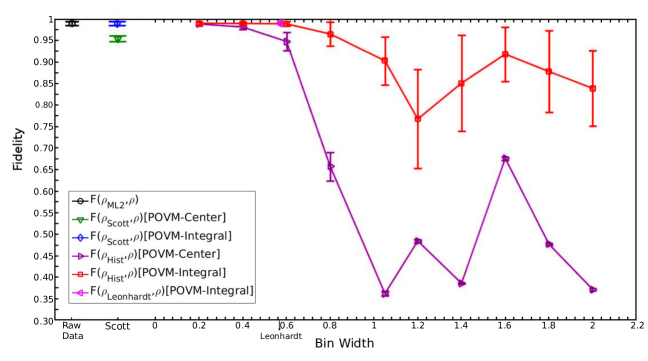
Figure 4: Average fidelity as a function of the bin width for a cat state with amplitude $\alpha=2$. The Hilbert space is truncated at $t=15$ photons. For this state, $\langle n\rangle=3.1978$, and $\overline{\langle\hat{n}\rangle}=3.1983$, giving a bin width by Leonhardt’s formula of $0.58$. The mean bin width for Scott’s method is $0.64$.

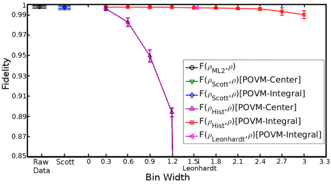
Figure 5: Average fidelity as a function of the bin width for a squeezed vacuum state whose squeezed quadrature has a variance 3/4 of the vacuum variance. The Hilbert space is truncated at $t=10$ photons. For this state, $\langle n\rangle=0.0167$, and $\overline{\langle\hat{n}\rangle}=0.0162$, giving a bin width by Leonhardt’s formula of $1.54$. The mean bin width for Scott’s method is $0.25$.

Until now, as mentioned before, every measurement outcome in a given bin has been associated with the measurement operator for the quadrature value at the center of that bin. That is, the measurement operator $\Pi_{i}$ associated with bin $i$ would give the probability density of obtaining a measurement result at the center of bin $i$ when computing $\mathrm{Tr}(\Pi_{i}\rho)$. Although this may be a useful approximation for very small bins, to improve our analysis, we now change each bin’s measurement operator so that it represents a measurement that occurs anywhere in the bin. To obtain these new operators, we numerically integrate the measurement operators over the width of each histogram bin. With these integrated measurement operators, computing $\mathrm{Tr}(\Pi_{i}\rho)$ will gives the probability to obtain a measurement result anywhere in bin $i$. We identify each case by adding $[$POVM-center$]$ and $[$POVM-integral$]$ to the legends in the graphs.

We also add to our analysis the use of the mean photon number estimate in Leonhardt’s formula, and we calculate the fidelity between $\rho_{\text{true}}$ and the state $\rho_{\mathrm{Leonhardt}}$ estimated using the resulting bin width. Recall that Leonhardt recommends that the bin width should be smaller than the one calculated using the maximum photon number in Eq. (8) but here we use the estimate of the mean photon number instead.

Figs. 3 and 4 show average fidelities as functions of the bin width for cat states with amplitudes $\alpha=1$ and $\alpha=2$, respectively. Fig. 5 examines a squeezed vacuum state whose squeezed quadrature has a variance 3/4 of the vacuum variance. Note for the cat states, as $\alpha$ increases, Scott’s bin width also increases, which is certainly undesirable because the quadrature distributions contain more fine structure. These graphs show that integrating the measurement operators over the width of each bin considerably improves the fidelities for all cases. We can also see that Leonhardt’s suggestion using the estimated mean photon number can be safely used as the upper bound for the bin width.

As seen in Eq. (7), Scott’s rule gives bin widths proportional to the sample standard deviation. Since states with a higher number of photons can have higher standard deviations, Scott’s method will produce larger bin widths. This is undesirable because pure states containing many photons have very fine features in their quadrature distributions. On the other hand, we expect Leonhardt’s method to perform better because it uses the estimated mean number of photons to calculate the bin width. We can clearly see the expected behavior of both methods for higher numbers of photons in Fig. 6, where we have used Fock states to check our claim.

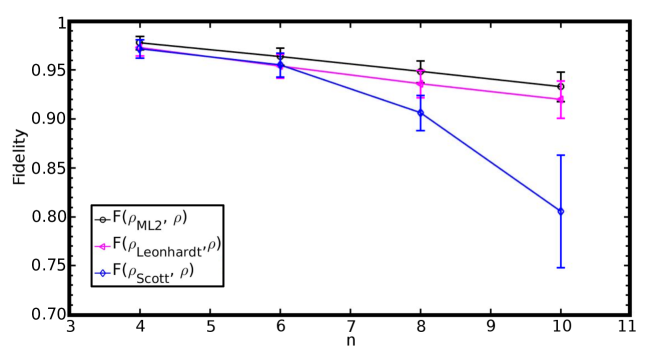
Figure 6: Average fidelities as functions of bin width for Fock states with different numbers of photons $n$. The bin widths from Leonhardt’s formula are 0.56 ($n=4$), 0.46 ($n=6$), 0.40 ($n=8$), and 0.36 ($n=10$). The mean bin width from Scott’s method are 0.69 ($n=4$), 0.82 ($n=6$), 0.95 ($n=8$), and 1.05 ($n=10$).

All of the discretization methods considered here give much faster fidelity estimates, as we can see in Figs. 7 and 8, with no significant loss of fidelity between the estimated states and the true states. The average times reported here include any calculations required to determine the desired bin width from the original homodyne data, the construction of histograms, and the ML density matrix estimation. All the simulations were carried out in a dual-core computer running at 3.7 GHz with 4 GB of RAM.

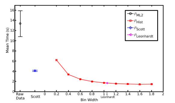
Figure 7: Average reconstruction time as a function of the bin width for a cat state with amplitude $\alpha=1$. The Hilbert space is truncated at $t=10$ photons. The mean bin width for Scott’s method is $0.35$, and the bin width given by Leonhardt’s formula is $1.05$.

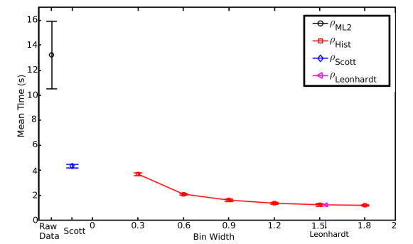
Figure 8: Average reconstruction time as a function of the bin width for a squeezed vacuum state whose squeezed quadrature has a variance 3/4 of the vacuum variance. The Hilbert space is truncated at $t=10$ photons. The mean bin width for Scott’s method is $0.25$, and the bin width given by Leonhardt’s formula is $1.54$.

VI Conclusion

We have used idealized numerical experiments to generate simulated data, performed maximum likelihood tomography on data sampled from cat states and squeezed vacuum states with and without discretization, and estimated the fidelities between the reconstructed states and the true state. We used two different methods to choose the bin width: Scott’s and Leonhardt’s methods. We studied using measurement operators calculated using the quadrature exactly at the center of each bin and integrating the measurement operators along the length of the bin.

Scott’s method calculates an optimal bin width, for each phase, based on the size and the standard deviation of the sample. This method works well for Gaussian states and states with small numbers of photons. States with higher number of photons have quadrature distributions with higher standard deviations, giving bigger bin widths for each phase. We implemented Scott’s method for Gaussian distributions, but if one has prior knowledge about the state and its distribution, one could tailor Scott’s rule by using more appropriate distributions in Eq. (5).

Leonhardt’s method recommends a bin width narrower than $q_{n}/2$, where $q_{n}$ decreases with the square root of the number of photons in the state being reconstructed. Since, in a real experiment, we do not know the mean number of photons in the state considered, we estimate the mean photon number from the quadrature measurement results. We have found that the method to find the mean number of photons from the quadrature measurement results gives accurate results. We checked that by comparing the estimated mean number of photons with the true mean number of photons for the cat states and squeezed vacuum states. We also have found that integrating the measurement operators over the width of each histogram bin significantly improves the fidelity. Using this strategy, Leonhardt’s formula safely establishes an upper bound to the bin width, and both methods provides a faster statistical estimation without losing too much information.