Political Discussion and Leanings on Twitter:
the 2016 Italian Constitutional Referendum

Abstract

The recent availability of large, high-resolution data sets of online human activity allowed for the study and characterization of the mechanisms shaping human interactions at an unprecedented level of accuracy. To this end, many efforts have been put forward to understand how people share and retrieve information when forging their opinion about a certain topic. Specifically, the detection of the political leaning of a person based on its online activity can support the forecasting of opinion trends in a given population. Here, we tackle this challenging task by combining complex networks theory and machine learning techniques. In particular, starting from a collection of more than 6 millions tweets, we characterize the structure and dynamics of the Italian online political debate about the constitutional referendum held in December 2016. We analyze the discussion pattern between different political communities and characterize the network of contacts therein. Moreover, we set up a procedure to infer the political leaning of Italian Twitter users, which allows us to accurately reconstruct the overall opinion trend given by official polls (Pearson’s $r=0.88$) as well as to predict with good accuracy the final outcome of the referendum. Our study provides a large-scale examination of the Italian online political discussion through sentiment-analysis, thus setting a baseline for future studies on online political debate modeling.

Introduction

In the last years, online social media have reached a fundamental role in the political discussion as they allow to easily spread a slogan or a political campaign in a large population of users. Every time we access a piece of information, share a content or comment on a news we leave a permanent digital trace, which can be used to infer our opinion regarding one particular event or topic Conover et al. (2011a, b); Ciulla et al. (2012). Among the variety of social media services, the micro-blogging platform Twitter is probably the most commonly used for political debate and by political leaders. This platform had a relatively recent diffusion in Italy, where it is used by nearly the $10\%$ of the Italian adult population and where the former prime minister Matteo Renzi was the first Italian politician to substantially found his public communication on tweets (the 140 characters-long messages published on Twitter). Also, Twitter stream of data is still available to the public through its application programming interface (API), making it the best candidate to study and describe the online political debates in a country.

In fact, previous works (mostly focused on the USA) found that the political discussion on Twitter can be a good proxy for the overall opinion of the population, and that Twitter data can therefore be used to infer the effects of a political event or to accurately predict the outcome of a vote Bovet et al. (2016). Moreover, several studies have highlighted the non-trivial dynamics of the opinions on Twitter and within political blogs, showing that politically active web users tend to aggregate in homogeneous communities, divided by political ideas, and avoiding discussion with the counterpart Vespignani (2009, 2012); Conover et al. (2011b, a).

In this work, we analyze the political debate on Twitter regarding the Italian Referendum Costituzionale (constitutional referendum) held on December the fourth, 2016. To this end, we firstly collected vote-related tweets during the intense political discussion that took place on social media during the three months before the vote. We then analyzed these tweets employing machine learning and network theory techniques. To the best of our knowledge, we are the first to apply sentiment-analysis to the political discussion on Twitter in the Italian scenario.

We aim at the detection of communities composed by interacting users and at characterizing the within-community homogeneity in terms of users opinions, investigating to which extent one community is influenced by users of other communities (outsiders). Additionally, we explore the possibility to use Twitter data as a reliable opinion poll and we assess their predictive power of the final outcome of the vote.

We found the Italian political discussion to be no different from the more studied USA case: strongly polarized communities act as echo-chambers and internally speak via retweets. On the other hand, the intercommunity discussion is mainly based on mentions used to report and criticize adversaries’ quotes. We also found that the temporal network structure generated by such contacts does react to major events happened during the political campaign. Examples include debates between the two major parties leaders held on TV and political or juridical events connected to the referendum.

The work is structured as follows: in Data Collection we describe the procedure adopted to retrieve the tweets and in Tweets classification the development of the classifier used to predict the leaning of each tweet in the dataset. From this vantage point, in User dynamical opinion we define a procedure to assign a dynamical opinion to a given user. These dynamical opinions are then used to characterize the time-varying network of contacts (Static characterization of the tweets network) and to identify the most influential spreaders of the online political debate (Network dynamics: influential spreaders identification). We further leverage on the reconstructed users opinion in Comparison with official polls, where we compare our recreated opinion trend to the empirical signal given by a large set of official polls, finding a very good agreement between the two. Finally, we draw the conclusions of our study.

Methods and Results

 

Data Collection

Starting from the midnight of the 30th of August 2016, we collected all the tweets in Italian containing one or more of the following strings: renzi, iovotono, iovotosi, referendum, referendumcostituzionale, bastaunsi, #NO, #SI, riformacostituzionale, m5s, pd, costituzione. Some of these strings are the keywords of the political campaign for the two main opposite formations (iovotono, iovotosi, bastaunsi, #NO, #SI) or the name of the two main political parties, while others may be linked to the political debate on the referendum. To filter out tweets written in languages other than Italian we relied on the automatic twitter language detection.

The collected tweets incorporate information on the author, the time of creation, the location (if available), the text content, the mentions (i.e., users cited in the text by inserting @username), the links and urls inserted, the hashtags, and the tweet kind. The latter specifies if the tweet is an original tweet (i.e. a new content generated by the user) or a retweet, meaning that the user reposted on its account a tweet previously generated by another user. A retweet contains a unique identifier of the original tweet being reposted, its original text and author. We did not reconstruct the follower network of the users (i.e., the network where two users are connected if one of the two is following the other) as we only use the single retweets/mentions as a proxy for the contact between individuals in the network. Data were recorded until the midnight of December the 4th 2016, right after the end of the consultation and the publication of the first exit polls. The resulting data set consists in $6\,894\,389$ tweets, authored by a total of $N_{users}=266\,437$ users.

Note that we did not filtered for accounts possibly associated to bots, i.e. accounts not run by humans but programmed to automatically post and share information. These are known to be part of the traffic volume Ratkiewicz et al. (2011); Ferrara et al. (2016); Suárez-Serrato et al. (2016), but here we assume that their net effect on the contact network is negligible.

Tweets classification

Given the political event under investigation, tweets need to be classified as belonging to one of four following classes: irrelevant, pro-no, neutral, and pro-yes. Following Salathé and Khandelwal (2011), we rely on supervised machine learning techniques to classify the tweets, for which we first needed an annotated data set to train a classifier. Manual classification was made by developing a simple web interface (shown in Figure 1 panel a) that prompts the user to classify each tweet into one of the four given categories. The information displayed to the user are: the text of the tweet, the contained hashtags, the author name, and all the urls included in the tweet.

Because of the sometimes ambiguous inclination of a tweet and the subjective perception of a tweet being more prone to the pro-yes or pro-no classes, we strengthened the manual classification of tweets by considering a tweet to be classified when i) it received at least 3 votes and ii) at least two thirds of them are in agreement. At the end of this procedure we ended up with a fairly balanced training set: out of the 1150 labeled tweets, 306 have been voted as irrelevant, 375 pro-no, 203 as neutral and the remaining 266 as pro-yes.

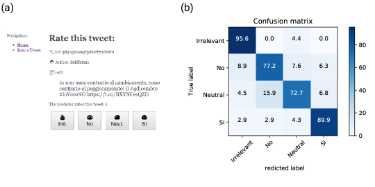
Figure 1: (a) The web interface presented to the human voter containing the unique identifier of the tweet in the database, the author’s nickname and the text of the tweet. If the tweet already features a preliminary classification, this is shown above the four buttons to classify the current tweet. Once the user inputs its preference, the system automatically presents a new tweet to be categorized. (b) The confusion matrix with percentage values for the random forest model with 21 estimators using the top 200 words and hashtags as features.

Sentiment-analysis

While previous works on the Italian scenario limited their attention to the volume of tweets containing fixed hashtags as a proxy for the overall volume of political affiliation Eom et al. (2015); Caldarelli et al. (2014), in this work we apply for the first time sentiment-analysis to Twitter data in the Italian political discussion. Although the former approach is certainly pioneering, it has several counter-effects. For example, a pro-yes tweet containing the official pro-no hashtag would straightforwardly increase the pro-no volume. Our method, detailed in the following, overcomes such difficulties.

The features of our model are the low-case words extracted from the text of the tweets where we removed punctuation and we substituted all the posted urls with their principal domain name (e.g., a link pointing to http://www.newspaper.it/politics/news_about_referendum is replaced by newspaper.it). Smileys are left as UTF-8 characters and we leave hashtags as separate entities, i.e. we do not treat them as simple words. This last choice can be justified a-posteriori by observing that the classifiers accuracy drops significantly when projecting hashtags to words by removing their leading pond #. We further process the features by stemming (using the WordNetLemmatizer from the nltk module of python Steven et al. (2009)) and removing the Italian stop-words from the corpus (using the stopwords collection from nltk.corpus). The resulting dictionary is composed by 535 different hashtags and 3773 words.

The manually annotated data set is used to train and validate three different classifiers: logistic regression, naive Bayes, and random forest Salathé and Khandelwal (2011); Abu-Mostafa et al. (2012). Results are then compared to choose the best-performing model. The performances of each model are evaluated using a 4-fold cross validation scheme: a fourth of the labeled tweets is randomly selected for validation and the remaining three fourths for training, and the procedure is repeated four times. The accuracy of a model is defined as the 4-fold average of the percentage of tweets in the validation set whose automatic classification correctly matches the manual one. The three classifiers give relatively similar performances: 80$\%$ accuracy for the random forest model, 82$\%$ accuracy for logistic regression and 79$\%$ accuracy for the naive Bayes classifier.

To gain better performances we further improved the random forest classifier by leveraging on the weights of the fitted model that naturally measure the importance of each word. The procedure is implemented as follows:

• we trained a random forest classifier using the 3773 words in our dictionary (hashtags excluded) as features. The model fitted in this way has relatively low predictive power, with accuracy $\sim 50\%$;

• we selected the top 200 words ranked by feature importance (the top 10 most predictive words are referendum, renzi, no, sì, riforma, m5s, salvini, paese, grillo);

• finally, we trained a random forest model using all the hashtags and the top 200 words as features, obtaining 86$\%$ accuracy using 21 estimators and an impurity split equal to $3.1\cdot 10^{-6}$.

The confusion matrix of the model on the annotated dataset is shown in Figure 1 panel b. The model was finally used to classify all the remaining tweets, resulting in $\approx 2.6M$ irrelevant, $\approx 1.7M$ pro-no, $\approx 1.1M$ neutral and $\approx 0.5M$ pro-yes tweets.

User dynamical opinion

In the current section, we show and discuss the procedure used to define the opinion of each user in each day of the data collection, based on the users’ classified tweets. We denote by $i\in\{1,\dots,N_{users}\}$ the index identifying a given user, by $T=97$ the length of the data set expressed in days, and by $t\in\{1,\dots,T\}$ a given day ($t=1$ corresponds to August 31st and $t=97$ to December the 4th, the date of the referendum). Then, we denote by $\mathrm{(Yes)}_{i,t}$ the number of pro-yes tweets posted at time $t$ by author $i$, while the quantity $\mathrm{(No)}_{i,t}$ is defined analogously. Note that tweets classified as irrelevant are considered equivalent to those classified as neutral in what follows.

We define the daily activity as the opinion that the user expresses the most in its daily tweets, namely

$$a_{i,t}=\begin{cases}+1&\quad\mathrm{if}~{}\mathrm{(Yes)}_{i,t}>\mathrm{(No)}_{i,t}\\ -1&\quad\mathrm{if}~{}\mathrm{(Yes)}_{i,t}<\mathrm{(No)}_{i,t}\\ 0&\quad\mathrm{if}~{}\mathrm{(Yes)}_{i,t}=\mathrm{(No)}_{i,t}\,.\end{cases}$$ (1)

Note that the third condition also implies that if user $i$ either posts only neutral/irrelevant tweets or does not tweet at all, then its daily activity is assumed to be neutral.

The daily activity defined in (1) is not suitable to represent a user’s opinion, because it only captures what the user tweeted on a given day. Indeed, it is reasonable to assume that a person maintains her/his opinion even though she/he does not declare it on Twitter every single day. For such a reason, we define an opinion function that maps the daily activity of user $i$ to $o_{i,t}$, the actual opinion of user $i$ at time $t$. To include a memory effect, the opinion of user $i$ is the projected weighted sum of its daily activity up to time $t$

$$o_{i,t}=p\Bigg{(}\sum_{s=0}^{t}w_{s,t}a_{i,s}\Bigg{)},$$ (2)

where the projection function $p$ is discussed below and the $w_{s,t}$ are exponentially decaying weights given by

$$w_{s,t}=\frac{e^{-(t-s)/K}}{\sum_{s=0}^{t}e^{-(t-s)/K}}.$$

Here, parameter $K$ gives an approximation of the typical number of days before $t$ that are taken into account when determining the opinion of the user. The intuition is that the more recent a tweet is, the more it affects the opinion value of the user.

The function $p$ projects the argument within the parenthesis in (2) onto the discrete opinion set $\{-1,0,+1\}$, and a natural choice for such projection is therefore the sign function. However, an undesirable drawback of setting $p(x)=\mathrm{sign}(x)$ is that even a mildly polarized user who tweeted in favor of, say, the yes vote on the very first day and then always posted neutral tweets for the following three months, would maintain a $+1$ opinion forever. Indeed, even though weights $w_{0,t}$ rapidly approach zero as $t$ becomes large, a sign $p$ function would still project the resulting small (but positive) sum on a pro-yes opinion. Then, we consider the projection to be a sign-like function with a $\epsilon$-widened preimage of zero, i.e.

$$p_{\epsilon}(x)=\begin{cases}-1&\mathrm{if}~{}x\in[-1,\epsilon]\\ 0&\mathrm{if}~{}x\in(-\epsilon,\epsilon)\\ +1&\mathrm{if}~{}x\in[\epsilon,1]\,.\end{cases}$$

Overall, two parameters are involved in the definition of the users opinion (2): the decaying time of the weights $K$ and $\epsilon$, the widening parameter of the projection function. Since we set the parameter $K$ to be the typical number of days that a user retains its opinion, we infer it from the data as follows. We fix $K$ to be the average number of days between two coherent tweets authored by the same user which are not separated by a differently classified tweet. Considering that on average users tweet coherently every $5$ days and $7$ hours (without showing any different daily activity in between), we deduce that the personal opinion is preserved for $K=5.29$ days on average. On the other hand, the role of the parameter $\epsilon$ is less self-evident. We recall that such parameter is introduced to allow users to return on a neutral position after a period of inactivity, but it actually has a more complex effect on the time evolution of the users opinion $o_{i,t}$ under several aspects. Here, we only report that the parameter is set to $\epsilon=0.075$ and we refer the reader to the Supplementary Material for a detailed discussion of its assessment.

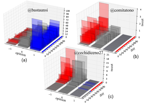
Figure 2: Histogram representation of the number of tweets authored by different users, subdivided in number of tweets classified as pro-no ($-1$, red), neutral or irrelevant ($0$, gray), and pro-yes ($+1$, blue). The coloured line on the right of each panel shows the resulting opinion of the user as defined in (2) with $K=5.29$ days and $\epsilon=0.075$. Panel (a) refers to the official pro-yes committee’s account (@bastaunsi), panel (b) to the official pro-no committee’s account (@comitatono), and panel (c) to user @cechidiceno27 that exhibits an opinion switch from a temporary pro-yes to a sustained pro-no leaning.

To illustrate the resulting opinion time course, we plotted the daily activity histograms of a few users and the resulting opinion time course in Figure 2. A detailed description of the figure content is given in the Supplementary Material.

Now that we defined the procedure to evaluate the opinion of each single user at a given time $t$ we can investigate how the topology of the network of contacts among Twitter users is shaped by the leaning of the users themselves.

Static characterization of the tweets network

Starting from our dataset of annotated tweets we build two different networks: i) the retweet network (RN), where a directed edge is drawn from user B to A when user A retweets user B, and ii) the mention network (MN), where we put a directed edge from user A to user B when A mentions B in a tweet. The two conventions on the edge direction are adopted so as to reproduce in the synthetic system the information flow found in the empirical social network.

The topology of this networks reflects the structure of the political debate within Twitter, and it is studied on two levels. First, we measure the size and track the evolution of the network connected components. We then detect the communities present in the system aiming at the analysis of their political polarization. Finally, we characterize the preferred mean of communication between communities with diverse average opinion.

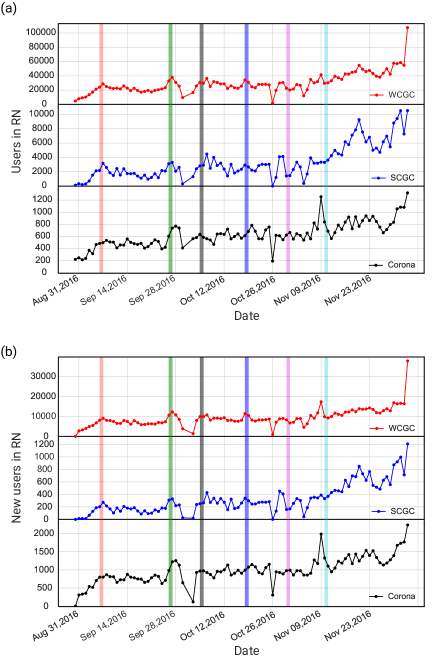
Figure 3: Connectivity of the RN. (a) Total number of users versus time in the WCGC, the SCGC and the corona. (b) Number of new users (i.e., users seen for the first time in the system) entering as part of the WCGC, the SCGC and the corona. The WCGC is an order of magnitude bigger than the SCGC, and approximately represents the entire network. The vertical bands represent some events that had a significant impact for the referendum debate: (red) the mayor of Rome, who previously endorsed the No, is involved in legal issues; (green) the Italian government fixes the referendum day; (black) the regional court of the region Lazio receive an appeal to invalidate part of the Referendum question formulation; (purple) the public debate about the referendum reaches the first pages of the main Italian newspapers; (pink) television debate with the Italian prime minister; (cyan) an important national meeting, Leopolda, organized by the Government party, is held in Florence.

Political communication network

To characterize the connectivity properties of the whole network, we study the weakly connected giant component (WCGC), the strongly connected giant component (SCGC) and the corona Bovet et al. (2016). The SCGC Dorogovtsev et al. (2001) is the core of a directed graph, and it is constituted of every pair of vertices that are connected in both directions. Thus, from one vertex in the SCGC one can approach any other vertex in the SCGC by moving either along or against the edge directions (interactions loop). The WCGC is a connected component formed by users that do not necessarily have reciprocal interaction with each other, whereas the corona is the rest of the network, i.e. it is formed by the smaller components of the network that do not belong to neither one of the giant components.

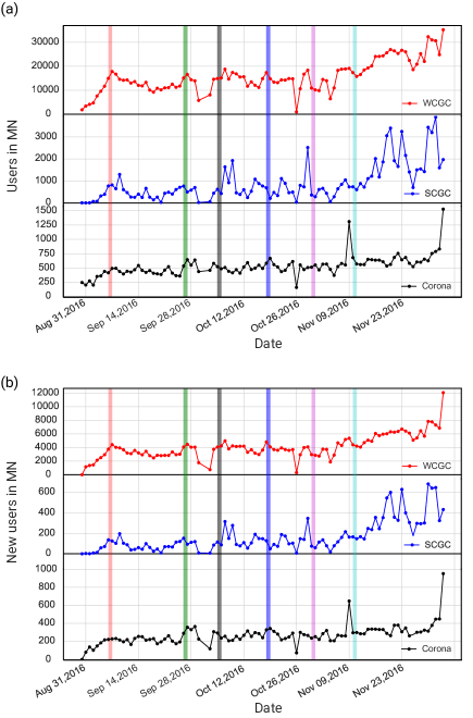
Figure 4: Connectivity of the MN. (a) Total number of users belonging to the WCGC, the SCGC and the corona as a function of time. (b) Number of new users entering the system in the WCGC, in the SCGC and the corona. The WCGC is an order of magnitude bigger than the SCGC, and it approximately represents the whole network. The vertical bands represent some significant events for the referendum debate, as described in the caption of Figure 3.

In the RN, the WCGC size ranges from $10^{3}$ to $4\times 10^{4}$ users, while the SCGC from $40$ to $1.6\times 10^{3}$, as shown in Figure 3. In the MN (see Figure 4), the WCGC have a size between $700$ and $1.7\times 10^{4}$, and the SCGC between $5$ and $10^{3}$. Thus, most of the entire set of nodes in both graphs belong to the WCGC (the coronas have an irrelevant size).

To understand how new users join the conversation, we show the number of users that appear for the first time in our network at each time step in Figure 3 panel b and Figure 4 panel b. As expected, most of the new users arrive in the WCGC and the corona. Indeed, new users are more likely to be less active in the discussion. As the referendum day approaches, both the SCGC size and the number of new users grow. We also observe different spikes in the number of both active and new users. These spikes correspond to particular dates, when important events stimulated the debate on the referendum (vertical bands in Figure 3 and Figure 4) triggering a clear response of the network. We elaborate further on this topic in the following sections.

Relation between network’s topology and users opinion

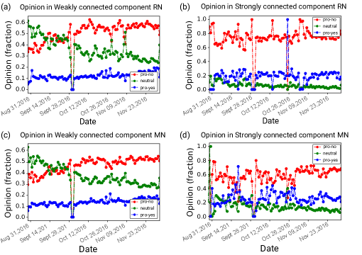
Figure 5: Top: average opinion in (a) the weakly connected and in (b) the strongly giant component in the RN. Bottom: average opinion in the (c) weakly connected component and in (d) the strongly giant component in the MN. The green dots are for the neutral opinion, red for the pro-no opinion, blue for the pro-yes opinion. Lines are guide to the eyes.

Given the network components found in the previous section we can now investigate how the users’ political opinion defined in User dynamical opinion is distributed within them. We find that the users with a neutral opinion are an important fraction of the weakly connected component for both the RN and MN (Figure 5 panels a and c). As one can reasonably expect, the number of neutral users decreases in time, as users opinions become more polarized while approaching the voting day. Additionally, polarized users tend to be more involved in interaction loops as it can be seen in Figure 5 panels b and d.

Community influencers and coherence

In order to gain further understanding of the political structure of the networks we implemented a community detection algorithm, applying the Louvain method Blondel et al. (2008). The Louvain algorithm is a greedy optimization method that finds the optimal division of a network into communities by iterative optimization of the network modularity, a measure of the density of links between nodes within a community with respect to the density of links outside it. The method returns a set of subgraphs more densely connected to one another than to other nodes, along with a hierarchy of communities at different scales.

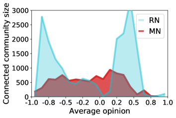
Figure 6: The size of communities plotted as a function of $\overline{O}_{C}$, the average opinion of users belonging to community $C$, for the RN (cyan area) and the MN (red area). In both cases, we show the $95$-th percentile of the community size distribution found for communities with a given average opinion.

Studying the size of the detected communities with respect to the average opinion inside the community gives an insight on the network political composition. We measure the average opinion $\overline{O}_{C}$ inside a community $C$ as the mean value of the opinion $o_{i,t}$ among the users belonging to the $C$ community and over the full observation period. Thus:

$$\overline{O}_{C}=\frac{1}{|C|T}\sum_{i\in C}\sum_{t=0}^{T}{o_{i,t}},$$ (3)

where $|C|$ is the number of nodes in community $C$. The result of such analysis are shown in Figure 6. In the RN the larger communities are those with a strongly polarized average opinion, whereas we find the communities in the MN to have a weaker opinion polarization, as the larger MN communities feature $\overline{O}_{C}\simeq 0$. Interestingly, we find the opinion polarization to be stronger for the pro-no communities of the RN. These communities are generally larger and more polarized (i.e. with more negative opinion) with respect to the ones supporting the pro-yes faction. Moreover, we observe also in the MN case a slight shift of the communities opinion toward the negative pole. This shift is reasonably due to the overall predominance of the pro-no side which were against the governing party (which was, on the contrary, promoting the pro-yes side).

Network dynamics: influential spreaders identification

After the analysis of the networks topology, it is worth considering how the edges arrangement and their activation patterns shape the evolution of a rumor spreading process unfolding on the network fabric. Specifically, in this section we quantitatively characterize the dynamics of a rumor spreading (RS) model on top of the mention and retweet networks. Since in a reaction-contact spreading model on a directed graphs each node (user) may spread and receive rumors only within the strongly connected component, we restrict our analysis to that subset only.

To perform the rumor spreading dynamics we define the unweighted temporal network (for both MN and RN), using the adjacency matrix $\mathbf{A}^{(t)}$ ($t=1,\dots,T$) where each non-zero entry is set equal to $1$. In Table 1 we show the relevant network properties for the undirected aggregated versions of the full and the SCGC graphs in both the MN and the RN. The high value of the second moment of the degree distribution, $\braket{k^{2}}$, observed in the two full graphs (in particular in the MN) highlights the rapid increase of the topological fluctuations, which corresponds to a high heterogeneity H Chen et al. (2012). This has important consequences on the dynamical processes as it implies a rapid decrease of the epidemic threshold in a corresponding standard infection process Barrat et al. (2008).

	Nodes	Edges	Density	D	C	$\braket{k}$	H
Full MN	80030	629061	$9.821\ 10^{-5}$	$\infty$	0.22	15.72	70.32
SCGC MN	15294	353867	$1.513\ 10^{-3}$	6	0.34	46.27	11.55
Full RN	179680	1543963	$4.782\ 10^{-5}$	$\infty$	0.11	17.19	47.19
SCGC RN	27437	917959	$1.219\ 10^{-3}$	7	0.28	66.91	8.56

Table 1: Statistical properties of the full and SCGC aggregated MN and RN: the diameter D, the clustering C, the average degree $\braket{k}$ and the degree heterogeneity H defined as $H=\braket{k^{2}}/\braket{k}^{2}$ Chen et al. (2012). All quantities are obtained using the undirected counterparts of both time-aggregated graphs.

Following Lentz et al. (2013), we compute the causal fidelity $c\in[0,1]$ of the SCGC graphs (see Supplementary Material). We find that $c=0.973$ and $c=0.979$ for the MN and RN, respectively. These values suggest that the temporal causality-driven effects in both SCGC networks are practically negligible. Thus, it is reasonable to characterize the rumor dynamics only considering the time-aggregated representations of the SCGC. Figure 7 panels a and b show the probability to find a path of length $t$ between two randomly chosen nodes, and the corresponding density of the accessibility graph. In spite of the networks directness, the density of the accessibility graph (black line) shows that after only half of the observation period (about 50 days) more than 80% of the network is causally connected. Therefore, the aggregated network representations give a good approximation of the temporal one, in accordance with the high causal fidelity. The shortest path length is broadly distributed for both the MN and RN, while its most frequent value is in both cases attained at a nine days long path. This means that the typical spreading time scales are of the order of 10 days.

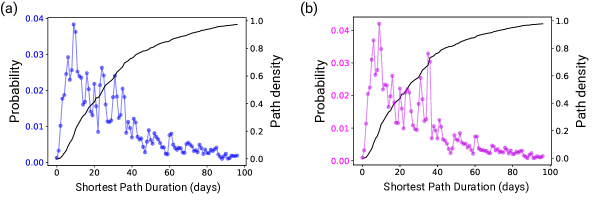
Figure 7: Distribution of the shortest path duration and the density $\rho(\mathbf{\mathcal{A}}^{T})$ of the accessibility graph (black) for (a) the SCGC of the MN (blue) and (b) the SCGC of the RN (violet). Causal fidelity values are $c=0.973$ and $c=0.979$ for the MN and the RN, respectively.

For the RS dynamics we consider the ignorant-spreader-stifler (ISS) model, with a single initial spreader per simulation. We focus on the Maki and Thomson ISS model Maki et al. (1973), where the rumor spreads via directed contacts. The directness feature of both MN and RN plays indeed a fundamental role in the corresponding evolution of the ISS dynamics as many users will never be able to spread a rumor that can reach a substantial portion of the network. The reaction dynamics for adjacent users is defined by the following spreading model Barrat et al. (2008)

$$\begin{cases}X+Y\xrightarrow{\beta}2Y\\ Y+Z\xrightarrow{\mu}2Z\\ Y+Y\xrightarrow{\mu}Z+Y\end{cases}$$ (4)

where $X^{(t)}$, $Y^{(t)}$ and $Z^{(t)}$ are the ignorant, spreader and stifler compartments, respectively, and the total population is $N=X^{(t)}+Y^{(t)}+Z^{(t)}$. In the Twitter case, spreaders correspond to users that have an information (such as a specific news about referendum) and if one spreader meet an ignorant user then the latter begins to spread this rumor as well. On the other hand, stiflers are users that lose interest in the news and persuade spreaders to stop propagating the rumor. Finally, the presence of two spreaders together could bring one of them to became a stifler. The two free parameters are the spreading (infection) and the stifler (recovery) rates $\beta$ and $\mu$. The main difference to the standard susceptible-infected-recovered (SIR) Anderson et al. (1992) model is the absence of spontaneous recovery: the transition to the stifler class may happen through a contact with another stifler or via a contact between two spreaders.

The problem of identifying the most influential nodes in a network, i.e. the so-called top spreaders, is a central issue in network science. Many works have addressed the question starting with the seminal paper of Kitsak et al. Kitsak et al. (2010), where the authors showed how the k-shell decomposition of the graph can give a much more elaborate description on how central a node is with respect to local measures. The lack of a satisfactory understanding of the problem comes from the high heterogeneity of the role played by the individual nodes in a complex network. Centrality measures are then used to quantitatively derive the importance of individual nodes Wasserman and Faust (1994).

Here we apply standard heuristic centrality metrics, namely the out-degree $k^{out}$, betweenness $b$ Freeman (1977), closeness $cl$, eigenvector centrality $e$ Bonacich (1972), k-core index $k_{c}$ Seidman (1983) and PageRank centrality $x$ Page et al. (1999). Other non-heuristics centrality measures (as the non-backtracking centrality Martin et al. (2014), which is supposed to match exactly the spreading capacity at criticality in the standard SIR model) cannot be used on directed networks. Because of the highly directed nature of both RN and MN we do not consider such metrics in what follows.

The high causal fidelity values found for the SCGC networks suggests to consider the topology as frozen during the time evolution of the system. The static assumption allows us to use standard static centrality measures to rank the users’ influence. Given a set of initial rumor spreaders (seeds), we are interested in quantifying the dependence of those seeds out-degree $k_{i}^{out}=\sum_{j}A^{T}_{ij}$ on the final outbreak size, varying $\beta$ and $\mu$. The natural measure of the nodes outbreak size is the spreading capacity $q_{i}$ of node $i$, defined as the average number of nodes in the stifler state (recovered) after the end of the infection process. This is defined as

$$q_{i}\equiv\lim_{t\rightarrow\infty}\braket{Z^{(t)}}_{i}/N\,,$$ (5)

where the average $\braket{\dots}_{i}$ is evaluated over $10^{2}$ different realization of the stochastic ISS dynamics described above, with the infection originating at node $i$.

The initial condition is of one spreader located at node $i$ and all other nodes ignorant. At each time step, the spreader nodes spread the rumor to their ignorant neighbors with probability $\beta$ and turn into a stifler with probability $\mu$ for each stifler neighbor. The dynamics stops when there are no more spreaders in the network.

We choose $\beta=0.1$ and $\mu=1.0$ as the reference observation point in the spreading parameter space, because is the closest at the decimal precision to the critical epidemic threshold, assuming that it is vanishing. The top 10 ranked users in terms of spreading capacity are presented in Table 2 for the MN and RN, respectively.

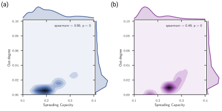
Figure 8: Kernel density estimation of the correlation between the distributions of the max-normalized spreading capacity $q/\max[q]$ and the out-degree $k^{out}/\max[k^{out}]$ for the aggregated SCGC MN (blue) and RN (violet). Parameters values for the spreading and recovery rates are respectively $\beta=0.1$ and $\mu=1.0$.

We found that the best performance metrics is the out-degree $k^{out}$, followed by the closeness centrality and the k-core index $k_{c}$ for both MN and RN. The Spearman’s rank correlation coefficient between the spreading capacity and the out-degree is shown in Figure 8. The value of the correlation coefficient for the complete $\beta$ range with unitary recovery is shown in Table 3.

Besides the very bad performance of PageRank, the best metric to rank the spreading ability of the users is the out-degree. Our results show a better performance of all metrics apart from PageRank in the MN, while the gap between the users’ number of retweets and the other metrics is smoothed in the RN. For the RN all metrics performed very poorly, which is probably due to the strong segregation of the network compared to the MN. In the latter instead, a local quantity such as the out-degree has proven to be sufficient to capture the rumor dynamics to a high level of accuracy, as it displays an almost perfect match with the spreading capacity ranking.

Rank	UserID (MN)	UserID (RN)
1	@DartSirius	@Dani_Gambit
2	@guffanti_marco	@nuccioaltieri
3	@lorenzo3107	@cadolo56
4	@Alessandro02088	@attanasio_g
5	@mdpennalunga	@GiuliaPozzuoli
6	@alessandrab72	@nonfraledonne
7	@onda_di_mare	@Bessico2
8	@angeloargento	@rpp_tweet
9	@fcerasani	@LaVarcaDiNoe
10	@pasqualegranata	@DCrognaletti

Table 2: Top 10 ranked users for their spreading capacity for $\beta=0.1$ and $\mu=1.0$ for the MN (left) and the RN (right).

	Mentions Network (MN)						Retweets Network (RN)
$\beta$	$k^{out}$	$b$	$cl$	$e$	$k_{c}$	$x$	$k^{out}$	$b$	$cl$	$e$	$k_{c}$	$x$
$0.1$	0.98	0.63	0.83	0.36	0.83	0.15	0.49	0.38	0.48	0.20	0.45	0.22
$0.2$	0.97	0.63	0.83	0.35	0.83	0.15	0.48	0.37	0.46	0.20	0.44	0.22
$0.3$	0.97	0.63	0.83	0.35	0.82	0.15	0.48	0.37	0.46	0.19	0.44	0.21
$0.4$	0.96	0.62	0.82	0.35	0.82	0.15	0.48	0.37	0.46	0.19	0.44	0.22
$0.5$	0.96	0.62	0.82	0.36	0.82	0.15	0.48	0.37	0.46	0.19	0.44	0.21
$0.6$	0.95	0.62	0.81	0.35	0.81	0.15	0.48	0.36	0.46	0.18	0.43	0.21
$0.7$	0.94	0.61	0.81	0.35	0.80	0.15	0.49	0.37	0.46	0.20	0.44	0.22
$0.8$	0.93	0.61	0.80	0.35	0.80	0.15	0.49	0.37	0.46	0.19	0.43	0.22
$0.9$	0.92	0.60	0.79	0.34	0.79	0.15	0.48	0.36	0.45	0.19	0.43	0.21
$1.0$	0.92	0.60	0.79	0.34	0.78	0.14	0.48	0.36	0.45	0.19	0.43	0.21

Table 3: Values of the Spearman’s rank correlation coefficient for the MN (left) and for the RN (right) in the full $\beta$ range at $\mu=1.0$ with the spreading capacity of the out-degree $k^{out}$, betweenness $b$, closeness $cl$, eigenvector $e$, k-core index $k_{c}$ and PageRank centrality $x$.

Comparison with official polls

In the current section, we compare the daily temporal evolution of the average opinion obtained from the Twitter dataset using the procedure described in User dynamical opinion and the opinion trend obtained through the official polls. The sources considered comprehend several sets of official polls (the whole dataset is reported in the Supplementary Material). These polls are carried out by different statistical research institutes and commissioned by different customers such as: the official website of the political and electoral polls of the Italian Government, popular Italian newspapers such as La Stampa, Il Corriere della Sera, and Il Sole 24 ore, and private monitoring companies. The sample size of the surveys is heterogeneous but always statistically significant, from a minimum of 400 to a maximum of 4000 individuals (about 1100 people interviewed on average). In addition, the time span of the official polls we considered goes from the 31th of August (the day we started collecting the data) to the 17th of November 2016, the day before the pre-election silence started.

In our analysis, we compare the daily average opinion $\langle o_{t}\rangle=N_{users}^{-1}\sum_{i=1}^{N_{users}}o_{i,t}$ with the official polls opinion, defined as the difference between the proportion of pro-yes and pro-no voters in each poll. In both the Twitter opinion and the official polls we considered also the undecided users. Note that the time span of the official polls is shorter than the Twitter one because the Italian law forces the official polls to stop two weeks before the vote. On the other hand, the Twitter data were recorded until the midnight of the 4th of December. Moreover, while the average opinion $\langle o_{t}\rangle$ measured from the tweets has a daily temporal resolution (as we project the daily user activity), the official polls do not have a regular frequency as they were generally published every couple of days.

Figure 9 shows the qualitative comparison, at the maximum temporal resolution, between $\langle o_{t}\rangle$ and the opinion reported by the official polls. In this plot, zero represent the perfect equilibrium between the pro-yes and pro-no voters and a positive or negative value of the average opinion represent respectively a majority of pro-yes or pro-no voters.

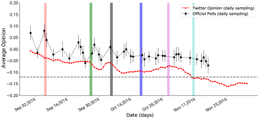
Figure 9: The daily comparison between the variable $\sum_{i=1}^{N_{users}}o_{i,t}$ (red) and the opinion obtained by official polls (black). The error bars on the official polls data represents the statistical error range given in each poll. The black dashed line represents the final result of the voting day $-0.12$. The vertical lines represent some important events for the referendum debate, as described in the caption of Figure 3.

We observe that during the first sampling period, from August 31th to September 20th, the average opinion obtained through the official polls fluctuates around zero, reaching a maximum of $0.09$ when the major of Rome, who endorsed the No, was involved in legal issues (red bar in Figure 9). On the other hand, the average opinion obtained through Twitter data starts near zero and then fundamentally decreases toward negative values. After the 20th of September, when the Italian government fixed the official voting day, the behaviour of the official polls starts to be more stable and prone to a pro-no vote. On the 5th of October, when the regional administrative court (tribunale amministrativo regionale, TAR) of region Lazio rejected a petition which had requested a partial invalidation of the referendum, the trend changes in both cases towards a more pro-yes political orientation. Subsequently, the two opinions approach more negative values until the 17th of November, when the official polls opinion is equal to $-0.07(\pm{0.03})$ while $\langle o_{t}\rangle=-0.13$.

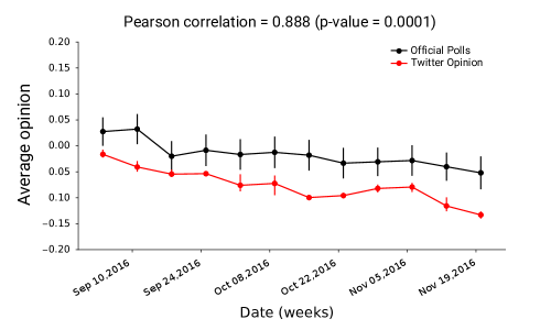
Figure 10: Average opinion per week in the Official Polls (black) and in the Twitter Opinion (red) datasets. The error bars on the Twitter opinion (red) represent the minimum and the maximum value obtained in each week, while the error bars of the official polls (black) are obtained as the average error per week.

Finally, to compare the different trends in a quantitative way we re-sampled the two time series averaging them with a weekly timescale. The resulting weakly average opinion for both datasets is showed in Figure 10. The error bars on the Twitter opinion (red line) represent the minimum and the maximum value obtained in each week, while the error bars of the official polls (black line) are obtained as the average error per week. The Pearson coefficient between the two time series is $r=0.888$ with a p-value equal to $p=10^{-4}$, showing a high degree of correlation between the two time series. Moreover, we find our latest reconstructed opinion value ($\langle o_{t}\rangle=-0.15$) to outperform the official polls in predicting the final referendum result. Indeed, given that $65.47\%$ of the eligible population voted and $40.88\%$ of this percentage voted Yes and the remaining $59.12\%$ voted No, the average opinion on the vote outcome is $-0.12$.

Conclusions

In this work we measured and characterized the discussion about a political event of national relevance in Italy using data from the Twitter microblogging platform.

We discussed the procedure implemented to collect tweets related to the Italian constitutional referendum, which allowed us to obtain a large amount of data for our analysis (approximately 7 millions tweets). Using a manually annotated subset of tweets, we trained a classifier able to predict the leaning of tweets with great accuracy ($86\%$ accuracy in a 4-fold cross validation). We deployed this classifier to predict the opinion of each user in the system given the user’s history and activity. Notably, our definition is dynamical so that the opinion of an user can change in time and it is not bound to a value computed at the end of the observation period.

Thanks to the dynamical opinion, we performed a characterization of the interaction network topology in terms of the average opinion. We found strongly polarized communities composed by users sharing the same opinion that internally interact with retweets, and that interact with other communities only by mentions.

The results are twofold: on the one hand they allow us to investigate the influential spreaders and the relevant nodes of the retweet and mention networks, while on the other hand they allow for a prediction of the population opinion trend. The former point is here achieved using the temporal network of interactions, thus without collecting the static network of friendships, an operation that turns out to be unfeasible on such large networks.

It is worth noting that the influential spreaders identified by our method are private users and not the official pro-yes and pro-no accounts as one would expect. From the ranking correlation of the rumor-spreading capacity of the active users, our analysis shows a clear out-performance of the out-degree over all other measures, in particular in the mention network. Although we did not perform extensive study of other relevant centralities measures defined specifically for undirected networks, such as non-backtracking centrality and random-walk accessibility, among the various measures we also find the k-core and closeness centrality as relevant for the identification of influential spreaders in social networks. Differently from previous finding De Arruda et al. (2014), in the social network of political discussion analyzed in this work, the simplest local measure of connectivity in the network, the out-degree $k^{out}$, is sufficient to estimate the correct ranking of users with extreme accuracy, and a correlation up to the value $r=0.98$, when approaching criticality.

Regarding the opinion trend, we found our estimate to be in good agreement with official polls. Our method is particularly interesting as it is significantly cheaper to track twitter activity rather than to finance a poll. Moreover, Italian laws prohibits companies and parties to perform and publish polls in the two weeks preceding a vote whereas, to the best of our knowledge, no restriction is currently given on Twitter data. It is therefore possible to track and characterize the general opinion dynamics in Twitter up to the date of an election, and for a longer time span with respect to the official surveys.

Besides the opinion trend, our analysis also allows for the identification of key-events influencing the overall opinion of the system. This can possibly provide for a real-time investigation of the response of the population to some public declarations or political events.

In conclusion, we developed a method to automatically collect and classify politically relevant tweets and analyze their political leaning. Also, we are able to evaluate the belonging of the users to certain discussion communities and their reaction to relevant political events. We also showed that our method gives a reliable prediction of the final outcome of the vote, serving this purpose even better than the official polls in the event considered.

Competing interests

The authors declare that no competing interests exist.

Author’s contributions

All authors conceived and designed the research project. All authors analyzed the data and wrote the paper. All authors contributed equally to this work.

Funding

This work has been founded by the DFG / FAPESP, within the scope of the IRTG 1740 / TRP 2015/50122-0.

I Defining $K$ and $\epsilon$

Qualitative analysis

To choose a proper value of $\epsilon$, we tested the outcome of the global process considering different values of $\epsilon$ in the interval $[0,0.1]$. First, we consider the percentage of users that forever maintain a polarized opinion after they assume one, who we name stubborn users. As hypothesized (see main text), Figure S1 panel a shows that the overall percentage halves when $\epsilon$ increases from zero to $0.01$, and it further reduces for larger values of the parameter. Another predictable effect of increasing $\epsilon$ is the reduction of the number of abrupt opinion jumps (i.e. direct switch from supporting Yes to supporting No, and vice versa). This is illustrated in Figure S1 panel b, which shows that the percentage of abrupt opinion jumps over the total amount of possible jumps slowly decreases as a function of $\epsilon$ (black dashed line), passing from about $0.1\%$ for $\epsilon=0$ to essentially zero percent for $\epsilon=0.1$. This is a desirable property as it seems rather unrealistic that a given user changes her/his mind all of a sudden, without passing through an intermediate neutral state before.

However, panel b in Figure S1 also reveals that the increase of both the number of opinion jumps towards a Yes vote (i.e. opinion jumps from No to Neutral and from Neutral to Yes, in red) and towards a No vote (from Yes to Neutral and from Neutral to No, in blue) largely counterbalance the reduction of abrupt jumps, yielding to a net increment in total number of jumps. As a consequence, the overall dynamics is less stable, resulting in users who change opinion more often for large values of $\epsilon$. In fact, also the maximum number of user’s opinion jumps among all users increases as a function of $\epsilon$, passing from twenty-five jumps for $\epsilon=0$ to a maximum number of over forty-five opinion jumps for $\epsilon=0.1$ (not shown in the picture). Although a richer and more complex dynamics might seem more interesting, it is rather unlikely that a person changes is mind this frequently. We draw the conclusion that $\epsilon$ should not be too large in order to reduce users’ flicking.

To summarize, in this section we demonstrated that the effect of increasing the parameter $\epsilon$ is, on the one hand, to reduce the users’ stubbornness (the tendency to maintain a given opinion once it is assumed). On the other hand, a larger value of $\epsilon$ results in a smaller number of abrupt jumps between Yes and No, at the cost of larger users’ opinion variability. However, we still lack a quantitative method allowing to asses the value of $\epsilon$ that produces a good trade-off between users’ stubbornness and opinion volatility.

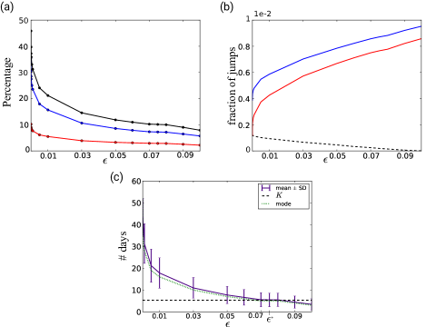
Figure S1: Global properties of the opinion dynamics defined in (2) as a function of $\epsilon$. (a) In red (blue), the percentage of users that forever maintain a $+1$ ($-1$) opinion after they first support Yes (No). In black, the sum of the two percentages. (b) The percentage of abrupt jumps (dashed black line) plotted against the percentage of jumps that approach Yes (red plain line) and the percentage of jumps that approach No (blue plain line). (c) Statistics of the number of days an opinion is maintained once it is assumed. The purple line shows the mean of such memory length and the associated vertical purple lines show the amplitude of the standard deviation. The dotted green line shows the mode, i.e. the value occurring most frequently. The horizontal black dashed line denotes the value of parameter $K=5.29$ days inferred from the dataset.

Quantitative analysis

To this aim, we observe that $\epsilon$ also has an effect on the memory of users’ past tweets. Indeed, since stubbornness and opinion retention are related, panel a in Figure S1 suggests that smaller values of $\epsilon$ result in longer users’ memory. In order to quantify such memory length, we considered the mean and the mode of the number of days an opinion is preserved once it is assumed. Such statistics are computed solely considering those users that acquired an opinion only once in the dataset, and then lost it. We decided not to consider users that assume and lose an opinion multiple times in order to focus on the effect of small clusters of Tweets which are frequent enough not to let the opinion vanish. Also, the requirement that the opinion has to be abandoned eventually rules out users that are ideologically polarized and would significantly extend the memory length statistics (an instance of ideologically polarized users are the official accounts represented in Figure 2 panels a and b).

In conclusion, Figure S1 panel c shows that only for $0.07<\epsilon<0.08$ the memory length is reasonably close the value of $K=5.29$ days which we identify in the main text. Hence, we analyzed the opinion dynamics of some users who only tweeted sporadically in favour of either Yes or No, and such analysis corroborated the choice of $\epsilon^{*}=0.075$.

As a synthetic description of the opinion resulting from the choice of $K=5.29$ days and $\epsilon=0.075$, in Figure S2 we show the empirical distribution (histogram) of the users’ time-averaged opinion

$$\bar{o}_{i}=T^{-1}\sum_{t=1}^{T}o_{i,t},\qquad i=1,\dots,N_{users}$$

which exhibits an evident skewness towards negative values (i.e. towards pro-no opinions).

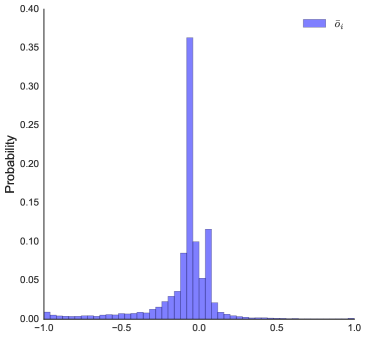
Figure S2: The distribution of the time average opinion of the users $\bar{o}_{i}$.

II Detailed description of the histograms in Figure 2

In Figure 2, the $y$-axis represents the time spanning from $t=1$ (31st August 2016) to $t=97$ (the date of the referendum), whereas the $z$-axis counts the number of tweets authored by the user on a specific day. Such histograms are subdivided according to how the tweets were classified. In fact, the $x$-axis contains the possible tweets classifications: $-1$ for a tweet supporting No (in red), $0$ for a neutral or irrelevant tweet (gray), and $+1$ for a tweet supporting Yes (blue).

Figure 2 panel a shows the histogram for the daily activity of the official pro-yes committee’s account @bastaunsi (twitter id 733695386846662657), whereas Figure 2 panel b represents one of the official pro-no committees’ account @comitatono (twitter id 696674734969397248). The line lying on the right side of the $xy$-plane shows the resulting user’s opinion time course, where blue stays for a pro-yes opinion, gray for a neutral opinion, and red for a pro-no opinion.

For both accounts we can observe a continuous twitting activity supporting the relative pole. As expected, such a sustained activity results in an opinion which is neutral at the beginning (neither of the accounts twitted on August 31st) but it changes for good once the first polarized tweet is posted. It is interesting to remark that the account @bastaunsi produced a much larger number of tweets than @comitatono, with a maximum of over one hundred tweets per days for the official pro-yes account versus a maximum of four tweets per day for the official pro-no account. Moreover, note that although the machine-learning algorithm classified some of @bastaunsi tweets as pro-no (note the red bars on the left of Figure 2 panel a), the large mole of pro-yes tweets allows to overlook what is likely to be a misclassification of the machine-learning algorithm.

Finally, Figure 2 panel c shows the daily activity histograms for account @cechidiceno27 (twitter id 780796377148162048). We observe that such user only started posting at $t=40$ (9th October 2016) with a pro-yes tweet, which resulted in a pro-yes opinion that lasted three days. Then, because of the repeated pro-no activity, its opinion returns to be neutral for a couple of days, just to settle definitively on a $-1$ opinion at $t=45$.

III Analysis of the temporal network for the rumor spreading dynamics and network centrality

The temporal nature of the dataset presents many challenges, first and foremost causality. To spread information from node $j$ to node $k$ at time $t^{\prime}=t+dt$, the same information must have already reached node $j$ from node $i$ at a previous time step $t<t^{\prime}$. Therefore the time-aggregation of the temporal networks can include paths of rumor propagation that are not present in the causally ordered temporal sequence of contacts. As it can be seen in Figure S3 panels a and b, the temporal activity of the SCGC (i.e. the fraction of nodes with at least one active edge at each time) is fluctuating during the whole time window.

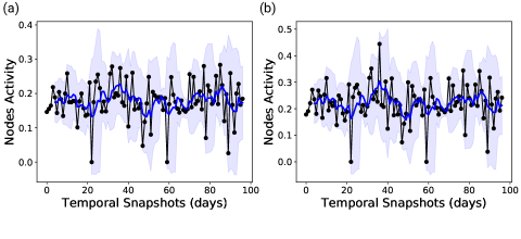
Figure S3: Fraction of active nodes in the temporal observation window of $T=97$ days for the SCGC MN (a) and SCGC RN (b). Two days with zero net activity were days of missed data collection.

To quantify the impact of causality driven by the temporal feature of the network, following Lentz et al. (2013), we compute the causal fidelity $c\in[0,1]$ of the SCGC graphs. The causal fidelity is defined as the fraction of the number of paths in the time-aggregated static network which can be also taken in the temporal one. Thus $c=\rho(\mathbf{\mathcal{A}}^{T})/\rho(\mathbf{A}^{T})$ where $\mathbf{\mathcal{A}}^{T}=\bigwedge_{t}^{T}(\mathbf{I}+\mathbf{A}^{(t)})$ and $\mathbf{A}^{T}=\bigvee_{t}^{T}\mathbf{A}^{(t)}$ are the full aggregated and accessibility boolean matrices obtained with the boolean product and sum respectively, and $\rho(\mathbf{A}^{(t)})=\sum_{ij}A^{(t)}_{ij}/N^{2}$ is the density of the $t$-th snapshot. The maximal causal fidelity $c=1$ implies that the temporal and static representations share the same path density. On the contrary, a low value of $c$ indicates that most of the paths in the static aggregate approximation do not follow a causal sequence of edges and thus do not belong to the temporal network. A fundamental quantity that we use in the main text is $\rho(\mathbf{A}^{(t)})-\rho(\mathbf{A}^{(t-1)})$ that gives the probability to find a path of length $t$, with $t=1,\dots,T$, between two randomly chosen nodes.

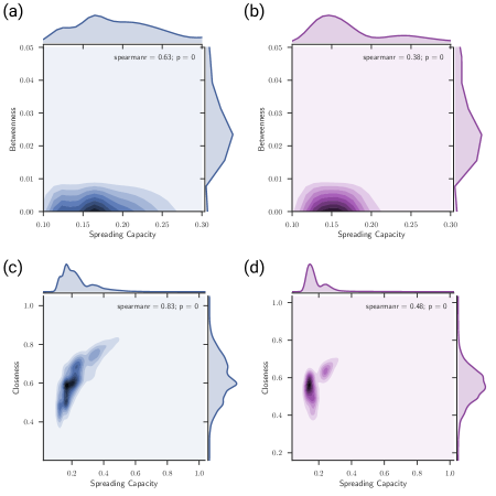
Figure S4: Kernel density estimation of the correlation between the distributions of the max-normalized spreading capacity $q/\max[q]$ and the max-normalized betweenness (top) and closeness (bottom) for the aggregated SCGC MN (blue) and RN (violet). Parameters values for the spreading and recovery rates are respectively $\beta=0.1$ and $\mu=1.0$.

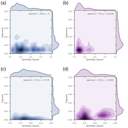
Figure S5: Kernel density estimation of the correlation between the distributions of the max-normalized spreading capacity $q/\max[q]$ and the max-normalized eigenvector (top) and PageRank (bottom) for the aggregated SCGC MN (blue) and RN (violet). Parameters values for the spreading and recovery rates are respectively $\beta=0.1$ and $\mu=1.0$.

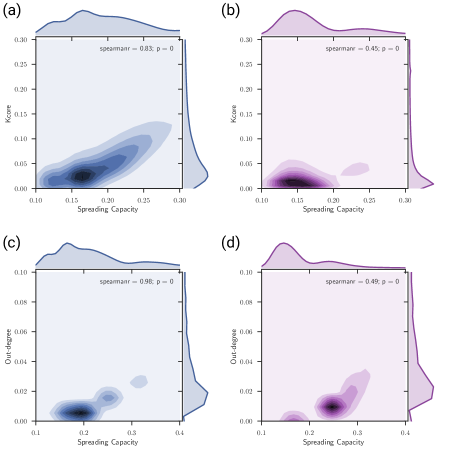
Figure S6: Kernel density estimation of the correlation between the distributions of the max-normalized spreading capacity $q/\max[q]$ and the max-normalized k-core (top) and out-degree (bottom) for the aggregated SCGC MN (blue) and RN (violet). Parameters values for the spreading and recovery rates are respectively $\beta=0.1$ and $\mu=1.0$.

We now briefly review the definition of the centrality measures used in the main text. For a detailed description see Newman (2010), for example.

The degree centrality $k$ is defined as the number of connections of each vertex. For a directed network we have the distinction between the in-degree and out-degree. The latter, which is relevant for our discussion, is the sum of each row of the adjacency matrix $A_{ij}$

$$k^{out}_{i}=\sum_{j}A_{ij}.$$ (S1)

The betweenness centrality $b$ is a measure of the amount of information transmitted by shortest paths along each node. It is defined as the fraction of shortest paths between all pairs of nodes that pass through node $i$

$$b_{i}=\sum_{kl}g_{kl}(i)/g_{kl},$$ (S2)

where $g_{kl}$ is the total number of shortest paths from node $k$ to node $l$ and $g_{kl}(i)$ is the number of these paths that also pass through node $i$.

The closeness centrality $cc$ is the reciprocal of the mean shortest-path length $l_{ij}$ from a node to all others

$$cc_{i}=N/\sum_{j}l_{ij}.$$ (S3)

The eigenvector centrality $e$ is defined by the components of the leading eigenvector of the adjacency matrix

$$e_{i}=\lambda_{1}^{-1}\sum_{j}A_{ij}e_{j},$$ (S4)

where $\lambda_{1}$ is the leading eigenvalue of $\mathbf{A}$.

The k-core decomposition of a graph is obtained from the subgraphs composed of nodes that have at least $k$ neighbors within the set itself for all possible values of the nodes degree $k$. For directed graphs one assumes that $k=k^{in}+k^{out}$. The k-core centrality $k_{c}$ of a node then equals the largest value of k-cores which the node belongs to.

Similarly to the eigenvector centrality the PageRank centrality $x$ is defined in terms of the spectra of the so-called Google matrix. PageRank can be computed iteratively from

$$x_{i}=\alpha\sum_{j}A_{ji}x_{j}/k_{j}^{out}+(1-\alpha)/N,$$ (S5)

where $\alpha=0.85$ is the teleportation parameter, which gives the probability to randomly relocate during a random-walk in the network.

In Figure S4,  S5  S6 we show the kernel density estimation of the spreading capacity with the centrality measures.

Figure S7: Circular representation of the strongly connected component of the aggregated network of mentions with the time average of the users’ opinions $\bar{o}_{i}$. The average opinion is represented here with color codes as blue (Yes) if $\bar{o}_{i}>0$ and red (No) if $\bar{o}_{i}\leq 0$, and analogously for the edges. The node’s ordering is given by the stochastic block model for community detection Decelle et al. (2011); Peixoto (2014a, b).

IV Official polls dataset

The official polls dataset is available in the file ReferendumOfficialPolls.csv.

References

- Conover et al. (2011a) M. D. Conover, B. Goncalves, J. Ratkiewicz, A. Flammini, and F. Menczer, in 2011 IEEE Third International Conference on Privacy, Security, Risk and Trust and 2011 IEEE Third International Conference on Social Computing (2011) pp. 192–199.
- Conover et al. (2011b) M. Conover, J. Ratkiewicz, M. R. Francisco, B. Gonçalves, F. Menczer, and A. Flammini, ICWSM 133, 89 (2011b).
- Ciulla et al. (2012) F. Ciulla, D. Mocanu, A. Baronchelli, B. Gonçalves, N. Perra, and A. Vespignani, EPJ Data Science 1, 8 (2012).
- Bovet et al. (2016) A. Bovet, F. Morone, and H. A. Makse, arXiv preprint arXiv:1610.01587 (2016).
- Vespignani (2009) A. Vespignani, Science 325, 425 (2009), http://science.sciencemag.org/content/325/5939/425.full.pdf .
- Vespignani (2012) A. Vespignani, Nature physics 8, 32 (2012).
- Ratkiewicz et al. (2011) J. Ratkiewicz, M. Conover, M. Meiss, B. Gonçalves, S. Patil, A. Flammini, and F. Menczer, in Proceedings of the 20th international conference companion on World wide web (ACM, 2011) pp. 249–252.
- Ferrara et al. (2016) E. Ferrara, O. Varol, C. Davis, F. Menczer, and A. Flammini, Communications of the ACM 59, 96 (2016).
- Suárez-Serrato et al. (2016) P. Suárez-Serrato, M. E. Roberts, C. Davis, and F. Menczer, in International Conference on Social Informatics (Springer, 2016) pp. 269–278.
- Salathé and Khandelwal (2011) M. Salathé and S. Khandelwal, PLOS Computational Biology 7, 1 (2011).
- Eom et al. (2015) Y.-H. Eom, M. Puliga, J. Smailović, I. Mozetič, and G. Caldarelli, PloS one 10, e0131184 (2015).
- Caldarelli et al. (2014) G. Caldarelli, A. Chessa, F. Pammolli, G. Pompa, M. Puliga, M. Riccaboni, and G. Riotta, PloS one 9, e95809 (2014).
- Steven et al. (2009) B. Steven, E. Klein, and E. Loper, OReilly Media Inc (2009).
- Abu-Mostafa et al. (2012) Y. S. Abu-Mostafa, M. Magdon-Ismail, and H.-T. Lin, Learning From Data (AMLBook, 2012).
- Dorogovtsev et al. (2001) S. N. Dorogovtsev, J. F. F. Mendes, and A. N. Samukhin, Physical Review E 64, 025101 (2001).
- Blondel et al. (2008) V. D. Blondel, J.-L. Guillaume, R. Lambiotte, and E. Lefebvre, Journal of statistical mechanics: theory and experiment 2008, P10008 (2008).
- Chen et al. (2012) D. Chen, L. Lü, M.-S. Shang, Y.-C. Zhang, and T. Zhou, Physica a: Statistical mechanics and its applications 391, 1777 (2012).
- Barrat et al. (2008) A. Barrat, M. Barthelemy, and A. Vespignani, Dynamical processes on complex networks (Cambridge university press, 2008).
- Lentz et al. (2013) H. H. Lentz, T. Selhorst, and I. M. Sokolov, Physical review letters 110, 118701 (2013).
- Maki et al. (1973) D. P. T. Maki et al., Mathematical models and applications: with emphasis on the social life, and management sciences, Tech. Rep. (1973).
- Anderson et al. (1992) R. M. Anderson, R. M. May, and B. Anderson, Infectious diseases of humans: dynamics and control, Vol. 28 (Wiley Online Library, 1992).
- Kitsak et al. (2010) M. Kitsak, L. K. Gallos, S. Havlin, F. Liljeros, L. Muchnik, H. E. Stanley, and H. A. Makse, Nature physics 6, 888 (2010).
- Wasserman and Faust (1994) S. Wasserman and K. Faust, Social network analysis: Methods and applications, Vol. 8 (Cambridge university press, 1994).
- Freeman (1977) L. C. Freeman, Sociometry , 35 (1977).
- Bonacich (1972) P. Bonacich, Journal of Mathematical Sociology 2, 113 (1972).
- Seidman (1983) S. B. Seidman, Social Networks 5, 97 (1983).
- Page et al. (1999) L. Page, S. Brin, R. Motwani, and T. Winograd, The PageRank citation ranking: Bringing order to the web., Tech. Rep. (Stanford InfoLab, 1999).
- Martin et al. (2014) T. Martin, X. Zhang, and M. Newman, Physical review E 90, 052808 (2014).
- De Arruda et al. (2014) G. F. De Arruda, A. L. Barbieri, P. M. Rodríguez, F. A. Rodrigues, Y. Moreno, and L. da Fontoura Costa, Physical Review E 90, 032812 (2014).
- Newman (2010) M. Newman, Networks: an introduction (Oxford university press, 2010).
- Decelle et al. (2011) A. Decelle, F. Krzakala, C. Moore, and L. Zdeborová, Physical Review E 84, 066106 (2011).
- Peixoto (2014a) T. P. Peixoto, figshare (2014a), 10.6084/m9.figshare.1164194.
- Peixoto (2014b) T. P. Peixoto, Physical Review X 4, 011047 (2014b).
Supplementary Material

References

- Conover et al. (2011a) M. D. Conover, B. Goncalves, J. Ratkiewicz, A. Flammini, and F. Menczer, in 2011 IEEE Third International Conference on Privacy, Security, Risk and Trust and 2011 IEEE Third International Conference on Social Computing (2011) pp. 192–199.
- Conover et al. (2011b) M. Conover, J. Ratkiewicz, M. R. Francisco, B. Gonçalves, F. Menczer, and A. Flammini, ICWSM 133, 89 (2011b).
- Ciulla et al. (2012) F. Ciulla, D. Mocanu, A. Baronchelli, B. Gonçalves, N. Perra, and A. Vespignani, EPJ Data Science 1, 8 (2012).
- Bovet et al. (2016) A. Bovet, F. Morone, and H. A. Makse, arXiv preprint arXiv:1610.01587 (2016).
- Vespignani (2009) A. Vespignani, Science 325, 425 (2009), http://science.sciencemag.org/content/325/5939/425.full.pdf .
- Vespignani (2012) A. Vespignani, Nature physics 8, 32 (2012).
- Ratkiewicz et al. (2011) J. Ratkiewicz, M. Conover, M. Meiss, B. Gonçalves, S. Patil, A. Flammini, and F. Menczer, in Proceedings of the 20th international conference companion on World wide web (ACM, 2011) pp. 249–252.
- Ferrara et al. (2016) E. Ferrara, O. Varol, C. Davis, F. Menczer, and A. Flammini, Communications of the ACM 59, 96 (2016).
- Suárez-Serrato et al. (2016) P. Suárez-Serrato, M. E. Roberts, C. Davis, and F. Menczer, in International Conference on Social Informatics (Springer, 2016) pp. 269–278.
- Salathé and Khandelwal (2011) M. Salathé and S. Khandelwal, PLOS Computational Biology 7, 1 (2011).
- Eom et al. (2015) Y.-H. Eom, M. Puliga, J. Smailović, I. Mozetič, and G. Caldarelli, PloS one 10, e0131184 (2015).
- Caldarelli et al. (2014) G. Caldarelli, A. Chessa, F. Pammolli, G. Pompa, M. Puliga, M. Riccaboni, and G. Riotta, PloS one 9, e95809 (2014).
- Steven et al. (2009) B. Steven, E. Klein, and E. Loper, OReilly Media Inc (2009).
- Abu-Mostafa et al. (2012) Y. S. Abu-Mostafa, M. Magdon-Ismail, and H.-T. Lin, Learning From Data (AMLBook, 2012).
- Dorogovtsev et al. (2001) S. N. Dorogovtsev, J. F. F. Mendes, and A. N. Samukhin, Physical Review E 64, 025101 (2001).
- Blondel et al. (2008) V. D. Blondel, J.-L. Guillaume, R. Lambiotte, and E. Lefebvre, Journal of statistical mechanics: theory and experiment 2008, P10008 (2008).
- Chen et al. (2012) D. Chen, L. Lü, M.-S. Shang, Y.-C. Zhang, and T. Zhou, Physica a: Statistical mechanics and its applications 391, 1777 (2012).
- Barrat et al. (2008) A. Barrat, M. Barthelemy, and A. Vespignani, Dynamical processes on complex networks (Cambridge university press, 2008).
- Lentz et al. (2013) H. H. Lentz, T. Selhorst, and I. M. Sokolov, Physical review letters 110, 118701 (2013).
- Maki et al. (1973) D. P. T. Maki et al., Mathematical models and applications: with emphasis on the social life, and management sciences, Tech. Rep. (1973).
- Anderson et al. (1992) R. M. Anderson, R. M. May, and B. Anderson, Infectious diseases of humans: dynamics and control, Vol. 28 (Wiley Online Library, 1992).
- Kitsak et al. (2010) M. Kitsak, L. K. Gallos, S. Havlin, F. Liljeros, L. Muchnik, H. E. Stanley, and H. A. Makse, Nature physics 6, 888 (2010).
- Wasserman and Faust (1994) S. Wasserman and K. Faust, Social network analysis: Methods and applications, Vol. 8 (Cambridge university press, 1994).
- Freeman (1977) L. C. Freeman, Sociometry , 35 (1977).
- Bonacich (1972) P. Bonacich, Journal of Mathematical Sociology 2, 113 (1972).
- Seidman (1983) S. B. Seidman, Social Networks 5, 97 (1983).
- Page et al. (1999) L. Page, S. Brin, R. Motwani, and T. Winograd, The PageRank citation ranking: Bringing order to the web., Tech. Rep. (Stanford InfoLab, 1999).
- Martin et al. (2014) T. Martin, X. Zhang, and M. Newman, Physical review E 90, 052808 (2014).
- De Arruda et al. (2014) G. F. De Arruda, A. L. Barbieri, P. M. Rodríguez, F. A. Rodrigues, Y. Moreno, and L. da Fontoura Costa, Physical Review E 90, 032812 (2014).
- Newman (2010) M. Newman, Networks: an introduction (Oxford university press, 2010).
- Decelle et al. (2011) A. Decelle, F. Krzakala, C. Moore, and L. Zdeborová, Physical Review E 84, 066106 (2011).
- Peixoto (2014a) T. P. Peixoto, figshare (2014a), 10.6084/m9.figshare.1164194.
- Peixoto (2014b) T. P. Peixoto, Physical Review X 4, 011047 (2014b).