Non-stationary localized oscillations of an infinite string, with time-varying tension, lying on the Winkler foundation with a point elastic inhomogeneity

Abstract

We consider non-stationary oscillations of an infinite string with time-varying tension. The string lies on the Winkler foundation with a point inhomogeneity (a concentrated spring of negative stiffness). In such a system with constant parameters (the string tension), under certain conditions a trapped mode of oscillation exists and is unique. Therefore, applying a non-stationary external excitation to this system can lead to the emergence of the string oscillations localized near the inhomogeneity. We provide an analytical description of non-stationary localized oscillations of the string with slowly time-varying tension using the asymptotic procedure based on successive application of two asymptotic methods, namely the method of stationary phase and the method of multiple scales. The obtained analytical results were verified by independent numerical calculations based on the finite difference method. The applicability of the analytical formulas was demonstrated for various types of external excitation and laws governing the varying tension. In particular, we have shown that in the case when the trapped mode frequency approaches zero, localized low-frequency oscillations with increasing amplitude precede the localized string buckling. The dependence of the amplitude of such oscillations on its frequency is more complicated in comparison with the case of a one degree of freedom system with time-varying stiffness.

1 Introduction

In this paper we consider a mechanical system with mixed spectrum of natural oscillations. Namely, we deal with an infinite string with slowly time-varying tension. The string lies on the Winkler foundation with a point inhomogeneity (a concentrated spring of negative stiffness). In the case of a constant string tension the discrete part of the spectrum for such a system may contain unique (positive) eigenvalue, which is less than the lowest frequency for the string on the uniform foundation. This special natural frequency corresponds to a trapped mode of oscillation with eigenform localized near the spring. The phenomenon of trapped modes was discovered in the theory of surface water waves ursell1951trapping . The examples of various mechanical systems, where trapped modes can exist, can be found in studies kaplunov1986torsional ; abramyan1992characteristics ; kaplunov1995simple ; abramyan1998trapping ; Gavrilov-2006-trans ; gavrilov2002etm ; alekseev2002vibration ; mciver2003excitation ; indeitsev2004localization ; porter2007trapped ; kaplunov2008example ; motygin2008trapping ; nazarov2010sufficient ; pagneux2013trapped ; porter2014trapped ; gavrilov2016trapped ; kaplunov2005localized ; Ind-book-R2E ; indeitsev2000resonance ; indeitsev2012motion ; wang2014vibration ; indeitsev2015localization ; indeitsev2016evolution ; gavrilov2017trapped ; shishkina2018non .

It is known kaplunov1986torsional ; gavrilov2002etm ; mciver2003excitation ; Ind-book-R2E ; indeitsev2016evolution ; gavrilov2017trapped ; shishkina2018non that applying non-stationary external excitation to a system possessing trapped modes leads to the emergence of undamped oscillations localized near the inhomogeneity. The large time asymptotics for such oscillation can be found gavrilov2002etm ; mciver2003excitation ; indeitsev2016evolution ; gavrilov2017trapped ; shishkina2018non by means of the method of stationary phase fedoruk1977 ; nayfeh1993 . Gavrilov in gavrilov2002etm ; Gavrilov-2006-trans suggested an asymptotic procedure based on successive application of two asymptotic methods, namely the method of stationary phase fedoruk1977 ; nayfeh1993 and the method of multiple scales nayfehperturbation ; nayfeh1993 that allows us to investigate non-stationary processes in perturbed systems, with slowly time-varying parameters, possessing trapped modes. In studies gavrilov2002etm ; Gavrilov-2006-trans the problem concerning non-uniform motion of a point mass along a taut string on the Winkler foundation was considered and solved. Note that later the same problem was reconsidered in paper gao2014exact by Gao, Zhang, Zhang, and Zhong in very particular case of uniform motion at a given speed.

The asymptotic procedure suggested in gavrilov2002etm ; Gavrilov-2006-trans was successfully applied to describe the evolution of the amplitude of the trapped mode of oscillations in a taut string on the Winkler foundation with a point inertial inclusion of time-varying mass indeitsev2016evolution and in a taut string on the Winkler foundation with a concentrated spring of negative time-varying stiffness gavrilov2017trapped . All problems considered in previous papers gavrilov2002etm ; Gavrilov-2006-trans ; indeitsev2016evolution ; gavrilov2017trapped are formulated for the Klein-Gordon PDE with constant coefficients. In our recent paper shishkina2018non a Bernoulli-Euler beam on the Winkler foundation with a concentrated spring of negative time-varying stiffness is considered. In the latter case, a PDE with constant coefficients is also under consideration. This allows one to verify the obtained analytical results by reduction of the problem to a Volterra integral equation of the second kind with its kernel expressed in terms of the fundamental solution for the corresponding PDE. The integral equation can be easily solved numerically. This was done in all previous studies gavrilov2002etm ; Gavrilov-2006-trans ; indeitsev2016evolution ; gavrilov2017trapped ; shishkina2018non , and a good mutual agreement between asymptotic and numeric results was demonstrated.

The consideration of the problem for a string with variable tension has some geophysical motivation gavrilov2016trapped . In contrast with previous papers gavrilov2002etm ; Gavrilov-2006-trans ; indeitsev2016evolution ; gavrilov2017trapped , the governing equation here is the Klein-Gordon equation with time-varying coefficients. To verify the obtained analytical results we solve numerically the initial value problem for this PDE using the finite difference method and demonstrate the applicability of the analytical formulas for various types of external excitation and laws governing the varying tension. Some preliminary results concerning this problem were presented in a recent conference publication gavrilov2017trapped .

Finally, note that very similar problems for structures of finite length were considered in studies luongo2001mode ; abramyan2011oscillations ; abramian2014oscillations ; abramian2017oscillations .

2 Mathematical formulation

We consider transverse oscillation of an infinite taut string on the Winkler elastic foundation. The elastic foundation has a point inhomogeneity in the form of a concentrated spring of a negative stiffness. The schematic of the system is shown in Figure 1.

Figure 1: The schematic of the system

Introduce the following notation: $u(x,t)$ is the displacement of a point of the string at the position $x$ and time $t$, $\mathscr{T}_{0}(t)>0$ is the string tension (a given function of time), $\rho>0$ is the mass of the string per unit length, $K_{0}$ is the absolute value for the stiffness $-K_{0}$ of the concentrated spring, $k_{0}>0$ is the stiffness for the Winkler foundation, $P_{0}(t)$ is the unknown force on the string from the spring, $p_{0}(t)$ is the given external force on the string. Quantities $k_{0}$, $K_{0}$, $\rho$ are constants. One can choose any orthogonal to the string direction, where $u(x,t),\ p_{0}(t)$ and $P_{0}(t)$ are assumed to be positive.

The governing equations are

$$\mathscr{T}_{0}(t)\,u_{xx}-\rho u_{tt}-k_{0}u=-P_{0}(t)\,\delta(x),$$ (1)

$$P_{0}(t)=K_{0}u(0,t)+p_{0}(t).$$ (2)

Here $\delta$ is the Dirac delta-function.

Now we introduce the dimensionless variables

$$\tau=t\sqrt{k_{0}/\rho},\qquad\xi=x\sqrt{k_{0}/\hat{\mathscr{T}}_{0}}$$ (3)

and rewrite governing equations (1), (2) in the following form

$$c^{2}(\tau)\,u^{\prime\prime}-\ddot{u}-u=-P(\tau)\,\delta(\xi),$$ (4)

$$P(\tau)=2u(0,\tau)+2p(\tau),$$ (5)

$$\hat{\mathscr{T}}_{0}=\frac{K_{0}^{2}}{4k_{0}},$$ (6)

$$c^{2}=\mathscr{T}_{0}/\hat{\mathscr{T}}_{0},\quad P=P_{0}/\sqrt{k_{0}\hat{\mathscr{T}}_{0}},\quad 2p=p_{0}/\sqrt{k_{0}\hat{\mathscr{T}}_{0}}.$$ (7)

Here and in what follows, we denote by prime the derivative with respect to spatial coordinate $\xi$ and by overdot the derivative with respect to time $\tau$. The quantity $c>0$ is the dimensionless transverse waves speed. The quantities $u,\ P,\ p$ remain dimensional ones having the dimension of length.

The initial conditions for Eq. (4) can be formulated in the following form, which is conventional for distributions (or generalized functions) Vladimirov1971 :

$$u\big{|}_{\tau<0}\equiv 0.$$ (8)

Note that according to Eqs. (4), (5), (8) we restrict ourselves to the important particular case of the general problem concerning non-stationary oscillation, where any external excitation (and, in particular, non-zero initial conditions) is applied only to the point of the string under the concentrated spring. One can take into account non-zero initial conditions

$$u(0,0)=0,\qquad \dot{u}(0,0)=2v_{0};$$ (9)

$$u(\xi,0)=0,\qquad \dot{u}(\xi,0)=0\qquad(\xi\neq 0);$$

for the velocity of the point under the concentrated spring, introducing of $p$ in the form of Vladimirov1971

$$p=v_{0}\delta(\tau)+\bar{p}(\tau).$$ (10)

Here $\bar{p}(\tau)$ is a non-singular at $\tau=0$ function such that $\bar{p}(\tau)\big{|}_{\tau<0}\equiv 0$.

The problem under consideration (4), (5), (8) is symmetric with respect to $\xi=0$. Integrating (4) over $\xi=0$ results in the following condition

$$[u^{\prime}]=-\frac{P(\tau)}{c^{2}(\tau)}=-\frac{2u(0,\tau)+2p(\tau)}{c^{2}(\tau)}.$$ (11)

Here, and in what follows, $[\mu]\equiv\mu(\xi+0)-\mu(\xi-0)$ for any arbitrary quantity $\mu$. Due to symmetry one has $[u^{\prime}]=2u^{\prime}(\xi+0)$. Thus, the problem for infinite string can be equivalently reformulated as the problem for homogeneous equation

$$c^{2}(\tau)\,u^{\prime\prime}-\ddot{u}-u=0$$ (12)

for $\xi>0$ with boundary condition at $\xi=0$

$$u^{\prime}(0,\tau)=-\frac{u(0,\tau)+p(\tau)}{c^{2}(\tau)}.$$ (13)

This equivalent formulation (12), (13), (8) is used for numerical calculations (Section 5).

3 A string with constant tension

In this section we consider the infinite string with a constant tension, thus $c=\operatorname{const}$.

3.1 Spectral problem

Put $p=0$ and consider the steady-state problem concerning the natural oscillations of the system described by Eqs. (4)–(5). Take

$$u=\hat{u}(\xi)\,\exp(-\mathrm{i}\Omega\tau).$$ (14)

Let us show that such a system possesses a mixed spectrum of natural frequencies. There exists a continuous spectrum of frequencies, which lies higher than the cut-off (or boundary) frequency: $|\Omega|\geq 1$. The modes corresponding to the frequencies from the continuous spectrum are harmonic waves. Trapped modes correspond to the frequencies from the discrete part of the spectrum, which lies lower than the cut-off frequency: $0<|\Omega|<1$. We want to demonstrate that for the problem under consideration the only one trapped mode can exist. Trapped modes are modes with finite energy, therefore, we require

$$\int_{-\infty}^{+\infty}\hat{u}^{2}\,\mathrm{d}\xi<\infty,\qquad\int_{-\infty}^{+\infty}\hat{u}^{\prime}{}^{2}\,\mathrm{d}\xi<\infty.$$ (15)

Now we substitute Eq. (14) into Eq. (4). This yields

$${\hat{u}}^{\prime\prime}-A^{2}(\Omega){\hat{u}}=-\frac{2{\hat{u}}(0)}{c^{2}}\,\delta(\xi),$$ (16)

where

$$A^{2}(\Omega)=\frac{1-\Omega^{2}}{c^{2}}.$$ (17)

Here, by definition, we assume that

$$A(\Omega)>0$$ (18)

for $0<\Omega<1$. The dispersion relation for the operator in the left-hand side of (16) is

$$\omega^{2}+A^{2}(\Omega)=0,$$ (19)

therefore, the wavenumber $\omega$ can be expressed as follows:

$$\omega=\pm\mathrm{i}A(\Omega).$$ (20)

The solution of Eq. (16), which satisfies (15), is

$$\hat{u}(\xi)={\hat{u}}(0)\,\frac{\exp(-A(\Omega_{0})|\xi|)}{c^{2}A(\Omega_{0})}.$$ (21)

Calculating the right-hand side of Eq. (21) at $\xi=0$ yields the frequency equation

$$c^{2}A(\Omega_{0})=1,$$ (22)

where $\Omega_{0}$ is the trapped mode frequency. Resolving the frequency equation results in

$$\Omega_{0}^{2}=1-{c}^{-2}.$$ (23)

Thus, according to (18), (22), (23) a trapped mode exists and is unique if and only if

$$c>1.$$ (24)

The critical value $c=1$ corresponds to possibility of localized buckling of the string.

Note that considering initial non-dimensionless problem for equations (4), (5) one can easily show gavrilov2017trapped that the trapped mode exists only if

$$K_{0}>0,$$ (25)

i.e. we deal with a destabilizing spring.

3.2 Inhomogeneous non-stationary problem

Put now $p\neq 0$. Applying to Eq. (4)–(5) the Fourier transform in time $\tau$ results in

$${u}_{F}^{\prime\prime}-A^{2}(\Omega){u_{F}}=-\frac{2}{c^{2}}\big{(}{u_{F}}(0,\Omega)+p_{F}(\Omega)\big{)}\,\delta(\xi),$$ (26)

where $u_{F}(0,\Omega),\ p_{F}(\Omega)$ are the Fourier transforms of $u(0,\tau)$ and $p(\tau)$, respectively. Resolving Eq. (26) with respect to $u_{F}(0,\Omega)$ and applying the inverse transform yields

$$u(0,\tau)=\frac{1}{2\pi}\int_{-\infty}^{+\infty}\frac{p_{F}e^{-\mathrm{i}\Omega\tau}\,\mathrm{d}\Omega}{c\sqrt{1-\Omega^{2}}-1}\\ =-\frac{1}{2\pi c^{2}}\int_{-\infty}^{+\infty}\frac{p_{F}(c\sqrt{1-\Omega^{2}}+1)e^{-\mathrm{i}\Omega\tau}\,\mathrm{d}\Omega}{\Omega^{2}-\Omega_{0}^{2}}.$$ (27)

At first, consider the simplest case $p=v_{0}\delta(\tau)$ ($p_{F}=v_{0})$ that corresponds to the initial conditions (9). To estimate asymptotically the integral in the right-hand side of (27) for large times $\tau$, we use the method of stationary phase fedoruk1977 ; nayfeh1993 . The principal part of the asymptotics is given by the contributions from poles

$$\Omega=\pm\Omega_{0}-\mathrm{i}0$$ (28)

of the amplitude function

$$\frac{c\sqrt{1-\Omega^{2}}+1}{\Omega^{2}-\Omega_{0}^{2}}.$$ (29)

The terms $-\mathrm{i}0$ in the right-hand side of (28) are taken in accordance with principle of limit absorption. Calculating the contributions from the poles fedoruk1977 ; Non-Stationary results in

$$u(0,\tau)=\frac{2v_{0}}{\Omega_{0}c^{2}}\sin\Omega_{0}\tau+O(\tau^{-3/2}),\quad\tau\to\infty.$$ (30)

One can prove kaplunov1986torsional that the principal part of the error term in (30) is given by the contribution from the boundary frequencies (the branching points) $\Omega=\pm 1$. Thus, for the large times, the non-stationary response of the system under consideration is undamped oscillations with the trapped mode frequency $\Omega_{0}$.

Now consider more general case when $p(\tau)$ is a vanishing as $\tau\to\infty$ function such that its Fourier’s transform $p_{F}(\Omega)$ does not have singular points on the real axis. Applying the method of stationary phase to the asymptotic evaluation of the integral in the right-hand side of (27) results in

$$u(0,\tau)=\frac{2|p_{F}(\Omega_{0})|}{\Omega_{0}c^{2}}\sin\big{(}\Omega_{0}\tau-\arg p_{F}(\Omega_{0})\big{)}+o(1),\\ \tau\to\infty.$$ (31)

The asymptotic order of the error term in the last formula depends on the properties of $p_{F}$.

4 A string with slowly varying tension

Assume that the string tension $\mathscr{T}_{0}$ and, therefore, the dimensionless transverse wave speed $c$ are slowly varying piecewise monotone function of the dimensionless time $\tau$: $c=c(\epsilon\tau)$. Here $\epsilon$ is a formal small parameter. We use an approach gavrilov2002etm ; Gavrilov-2006-trans ; indeitsev2016evolution based on the modification of the method of multiple scales nayfehperturbation (Section 7.1.6) for equations with slowly varying coefficients. The corresponding rigorous proof, which validates such asymptotic approach in the case of a one degree of freedom system, can be found in feschenko1967eng . We look for the asymptotics for the solution under the following conditions:

• $\epsilon=o(1),$

• $\tau=O(\epsilon^{-1}),$

• $c(\epsilon\tau)$ satisfies restriction (24) for all $\tau$.

To construct the particular solution of (4)–(5), which describes the evolution of the trapped mode of oscillation in the case of slowly varying $c$, we require that in the perturbed system

• Frequency equation (23) for the trapped mode holds for all $\tau$;

• Dispersion relation (19) at $\xi=\pm 0$ holds for all $\tau$.

Accordingly, we use the following ansatz ($\tau>0$, $\xi\lessgtr 0$):

$$u(\xi,\tau)=W(X,T)\,\exp\varphi(\xi,\tau),$$ (32)

$$T=\epsilon\tau,\quad X=\epsilon\xi,$$ (33)

$${\varphi}^{\prime}=\mathrm{i}\,\omega(X,T),\quad\dot{\varphi}=-\mathrm{i}\,\Omega(X,T),$$ (34)

$$W(X,T)=\sum_{j=0}^{\infty}\epsilon^{j}{W_{j}}(X,T).$$ (35)

Here the amplitude $W(X,T)$, the wavenumber $\omega(X,T)$, and the frequency $\Omega(X,T)$ are the unknown functions to be defined in accordance with Eq. (4). The variables $X,\ T,\ \varphi$ are assumed to be independent. Accordingly, we use the following representations for the differential operators:

$$\begin{gathered}\dot{(\cdot)}=-\mathrm{i}\,\Omega\,\partial_{\varphi}+\epsilon\,\partial_{T},\\ \ddot{(\cdot)}=-\Omega^{2}\,\partial^{2}_{\varphi\varphi}-2\epsilon\mathrm{i}\,\Omega\,\partial^{2}_{\varphi T}-\epsilon\mathrm{i}\,{\Omega^{\prime}}_{T}\,\partial_{\varphi}+O(\epsilon^{2}),\\ (\cdot)^{\prime}=\mathrm{i}\,\omega\,\partial_{\varphi}+\epsilon\,\partial_{X},\\ (\cdot)^{\prime\prime}=-\omega^{2}\,\partial^{2}_{\varphi\varphi}+2\epsilon\mathrm{i}\,\omega\,\partial^{2}_{\varphi X}+\epsilon\mathrm{i}\,{\omega}^{\prime}_{X}\,\partial_{\varphi}+O(\epsilon^{2}).\end{gathered}$$ (36)

We require that $\omega(X,T)$ and $\Omega(X,T)$ satisfy dispersion relation (19) and equation

$${\Omega}^{\prime}_{X}+{\omega}^{\prime}_{T}=0$$ (37)

that follows from (34). Since in the case of a string with constant tension the undamped oscillation can be described by Eq. (31), we assume that

$$\Omega(\pm 0,T)=\Omega_{0}(T).$$ (38)

Additionally, we require that

$$[W]=0,\qquad[\varphi]=0.$$ (39)

In Eq. (38) the right-hand side is defined in accordance with the frequency equation (22), wherein $c=c(T)$. The phase $\varphi(\xi,\tau)$ should be defined by the formula

$$\varphi=\mathrm{i}\int(\omega\,\mathrm{d}\xi-\Omega\,\mathrm{d}\tau).$$ (40)

For large times, integrating formally Eq. (4) with respect to $\xi$ over the infinitesimal vicinity of $\xi=0$ taking into account (5), one gets (11), wherein $p=0$. Now we substitute ansatz (32)–(35) and representations (36) into Eq. (11) and equate coefficients of like powers $\epsilon$. Taking into account frequency equation (22), and Eq. (38), one obtains that to the first approximation

$$[W_{0}{}^{\prime}_{X}]=0.$$ (41)

On the other hand, the quantity in the left-hand side of (41) can be defined by consideration of Eq. (4) at $\xi=\pm 0$. To do this, we substitute ansatz (32)–(35) and representations (36) into Eq. (4) and equate coefficients of like powers $\epsilon$. Taking into account dispersion relation (22) and Eq. (38), one obtains that to the first approximation

$$c^{2}(T)(2\omega\,{W_{0}}^{\prime}_{X}+{\omega}^{\prime}_{X}\,{W_{0}})+2\Omega_{0}\,{W_{0}}^{\prime}_{T}+{\Omega_{0}}^{\prime}_{T}\,{W_{0}}=0$$ (42)

at $\xi=\pm 0$. Due to (37) one has

$${\omega}^{\prime}_{X}={\omega}^{\prime}_{\Omega}\,\Omega^{\prime}_{X}=-{\omega}^{\prime}_{\Omega}\,{\omega}^{\prime}_{T},$$ (43)

where the right-hand side should be calculated in accordance with Eq. (20). Thus, Eqs. (42) and (43) result in

$${W_{0}}^{\prime}_{X}=-\frac{2\Omega_{0}\,{W_{0}}^{\prime}_{T}+(-c^{2}{\omega}^{\prime}_{\Omega}{\omega}^{\prime}_{T}+{\Omega_{0}}^{\prime}_{T})\,{W_{0}}}{2\mathrm{i}\gamma A(\Omega_{0},T)c^{2}(T)},$$ (44)

where $\gamma=\operatorname{sign}\xi$. Accordingly,

$${}[{W_{0}}^{\prime}_{X}]=-\frac{\Lambda_{2}{W}_{0}+\Lambda_{1}{W}_{0}{}^{\prime}_{T}}{\mathrm{i}A(\Omega_{0})c^{2}},$$ (45)

$$\Lambda_{1}\equiv 2\Omega_{0},$$ (46)

$$\Lambda_{2}\equiv c^{2}A^{\prime}_{\Omega}(\Omega_{0})A^{\prime}_{T}(\Omega_{0})+{\Omega_{0}}^{\prime}_{T},$$ (47)

where the right-hand side of Eq. (45) is taken at $\xi=0$.

Now, equating the right-hand sides of Eqs. (41) and (45) results in the first approximation equation for $\bar{W}_{0}(T)\equiv W_{0}(0,T)$:

$$\Lambda_{2}\bar{W}_{0}+\Lambda_{1}\bar{W}_{0}{}^{\prime}_{T}=0.$$ (48)

The general solution of the last equation is

$$\bar{W}_{0}=C_{0}\exp\Big{(}-\int\frac{\Lambda_{2}}{\Lambda_{1}}\,\mathrm{d}T\Big{)},$$ (49)

where $C_{0}$ is an arbitrary constant. Using (17), one gets

$$A^{\prime}_{\Omega}=-\frac{\Omega_{0}}{c\sqrt{1-\Omega_{0}^{2}}},$$ (50)

$$A^{\prime}_{T}=-\frac{\Omega_{0}\Omega_{0}{}^{\prime}_{T}}{c\sqrt{1-\Omega_{0}^{2}}}-\frac{c{}^{\prime}_{T}}{c^{2}}\sqrt{1-\Omega_{0}^{2}}.$$ (51)

Substituting these expressions into (47) yields

$$\Lambda_{2}=\frac{\Omega^{2}_{0}{\Omega_{0}}^{\prime}_{T}}{1-{\Omega}^{2}_{0}}+\frac{\Omega_{0}c^{\prime}_{T}}{c}+{\Omega_{0}}^{\prime}_{T}.$$ (52)

Therefore,

$$-\int\frac{\Lambda_{2}}{\Lambda_{1}}\,\mathrm{d}T=-\int\frac{\mathrm{d}\Omega^{2}_{0}}{4\left(1-{\Omega}^{2}_{0}\right)}-\int\frac{\mathrm{d}c}{2c}-\int\frac{\mathrm{d}\Omega_{0}}{2\Omega_{0}}\\ =\frac{1}{4}\ln\left(1-{\Omega}^{2}_{0}\right)-\frac{1}{2}\ln c-\frac{1}{2}\ln\Omega_{0}.$$ (53)

Substituting the last equation into the right-hand side of Eq. (49) yields the final result

$$\bar{W}_{0}=C_{0}\frac{\left(1-{\Omega}^{2}_{0}\right)^{1/4}}{\left(c\Omega_{0}\right)^{1/2}}.$$ (54)

Taking into account (23), one can rewrite the last formula in two equivalent forms:

$$\bar{W}_{0}=\frac{C_{0}}{\sqrt{c}\,(c^{2}-1)^{1/4}}=C_{0}\sqrt{\frac{1-\Omega_{0}^{2}}{\Omega_{0}}}$$ (55)

If $\Omega_{0}\to+0$ (or, equivalently, $c\to 1+0$, $\mathscr{T}_{0}\to\frac{K_{0}^{2}}{4k_{0}}+0$), then

$$\bar{W}_{0}=\frac{C_{0}}{\Omega_{0}^{1/2}}+o(1).$$ (56)

Hence, localized low-frequency oscillations with increasing amplitude precede the localized string buckling.

This result is analogous to the classical result for a one degree of freedom system

$$\ddot{y}+\hat{\varOmega}^{2}(\epsilon\tau)y=0,$$ (57)

where the following formula

$$Y\propto\frac{1}{\hat{\varOmega}^{1/2}}$$ (58)

for the amplitude of free oscillations $Y$ is valid (the Liouville – Green approximation nayfehperturbation ). On the other hand, unlike one degree of freedom system (57), for the system under consideration, formula (56) is valid only in the limiting case $\Omega_{0}\to+0$. For finite $\Omega_{0}$ the dependence (55) is more complicated.

Combining the solution in the form of Eqs. (32)–(35) with its complex conjugate, we get the non-stationary solution as the following ansatz:

$$u(0,\tau)\sim\bar{W}_{0}\big{(}\Omega_{0}(T)\big{)}\sin\left(\int_{0}^{\tau}\Omega_{0}(T)\,\mathrm{d}T-D_{0}\right),$$ (59)

where $\bar{W}_{0}$ is defined by (55). The unknown constants $C_{0}$ and $D_{0}$ should be defined by equating the right-hand sides of (31) and (59) taken at $\tau=0$. This yields

$$C_{0}=\frac{2(c^{2}(0)-1)^{1/4}}{\Omega_{0}(0)c^{3/2}(0)}\,\big{|}p_{F}\big{(}\Omega_{0}(0)\big{)}\big{|}\\ =\frac{2\big{|}p_{F}\big{(}\Omega_{0}(0)\big{)}\big{|}}{c(0)(1-c^{-2}(0))^{1/4}},$$ (60)

$$D_{0}=\arg p_{F}\big{(}\Omega_{0}(0)\big{)}.$$ (61)

In the particular case $p=v_{0}\delta(\tau)$ that corresponds to the initial conditions (9) one has

$$C_{0}=\frac{2v_{0}\big{(}c^{2}(0)-1\big{)}^{1/4}}{\Omega_{0}(0)c^{3/2}(0)}=\frac{2v_{0}}{c(0)(1-c^{-2}(0))^{1/4}},$$ (62)

$$D_{0}=0.$$ (63)

In the particular case

$$p(\tau)=\bar{p}_{0}H(\tau)\exp(-\lambda\tau),$$ (64)

where $H(\tau)$ is the Heaviside function, $\bar{p}_{0}=\operatorname{const}$, and $\lambda=\mathrm{const}>0$, one has

$$p_{F}\big{(}\Omega_{0}(0)\big{)}=\frac{\bar{p}_{0}}{\lambda-\mathrm{i}\Omega_{0}(0)},$$ (65)

$$\big{|}p_{F}\big{(}\Omega_{0}(0)\big{)}\big{|}=\frac{|\bar{p}_{0}|}{\sqrt{\lambda^{2}+\Omega_{0}(0)^{2}}},$$ (66)

$$\arg\big{(}p_{F}\big{(}\Omega_{0}(0)\big{)}\big{)}=\arctan\frac{\Omega_{0}(0)}{\lambda}.$$ (67)

Finally, using in the case $p=v_{0}\delta(\tau)$ approximate asymptotically incorrect formula (56) instead of correct formula (55) yields

$$C_{0}=\frac{2v_{0}}{\sqrt{\Omega_{0}(0)}\,c^{2}(0)}=\frac{2v_{0}}{{\big{(}1-c^{-2}(0)\big{)}^{1/4}}\,{c^{2}(0)}}$$ (68)

together with formula (63).

5 Numerics

In previous studies gavrilov2002etm ; Gavrilov-2006-trans ; indeitsev2016evolution ; gavrilov2017trapped we dealt with several problems for the linear Klein-Gordon equation with constant coefficients. Numerical solutions were obtained by means of the reduction of the corresponding problem to an integral Volterra equation of the second kind with its kernel expressed in terms of the fundamental solution of the Klein-Gordon equation. This cannot be done for the problem under consideration in this paper, since now we deal with an equation with time-varying coefficients. To perform the numerical calculations we use SciPy software.

To verify constructed analytical solution (54) we solve numerically the initial value problem for PDE (12) with boundary condition (13) using the finite difference method. To discretize PDE (12) we use the following implicit difference scheme:

$$(c^{i})^{2}\frac{u_{j+1}^{i}-2u_{j}^{i}+u_{j-1}^{i}}{(\Delta\xi)^{2}}\\ -\frac{u_{j}^{i+1}-2u_{j}^{i}+u_{j}^{i-1}}{(\Delta\tau)^{2}}-\frac{u_{j}^{i+1}+u_{j}^{i-1}}{2}=0,$$ (69)

where integers $i,\ j$ ($0\leq j\leq N,\ -1\leq i$) are such that

$$u_{j}^{i}=u(j\Delta\xi,i\Delta\tau),$$ (70)

$$c^{i}=c(i\Delta\tau).$$ (71)

This scheme conserves donninger2011numerical ; strauss1978numerical the discrete energy for a nonlinear Klein-Gordon equation with constant coefficients. Numeric boundary conditions that correspond to (13) are taken in the form strikwerda2004finite

$$(c^{i+1})^{2}\frac{-3u_{0}^{i+1}+4u_{1}^{i+1}-u_{2}^{i+1}}{2\Delta\xi}\\ +(c^{i-1})^{2}\frac{-3u_{0}^{i-1}+4u_{1}^{i-1}-u_{2}^{i-1}}{2\Delta\xi}\\ +{(u_{0}^{i+1}+u_{0}^{i-1})}+(p^{i+1}+p^{i-1})=0.$$ (72)

At the right end we use boundary condition trangenstein2009numerical

$$u^{i}_{N}=u^{i}_{N-1}$$ (73)

that corresponds to the physical boundary condition $u^{\prime}=0$. Actually, the specific form of this boundary condition is not very important in our calculations, since we consider the discrete model of the string with sufficiently large length such that the wave reflections at the right end do not occur.

Numerical initial conditions are

$$u^{0}_{j}=u^{-1}_{j}=0.$$ (74)

All numerical results below are obtained for the case

$$\Delta\xi=0.025,\qquad\Delta\tau=0.01.$$ (75)

The dimensional coefficients $v_{0}$ and $\bar{p}_{0}$ are taken as $1\,\mathrm{m}$ and skipped in what follows for the aim of simplicity. Calculating the numerical solutions, which corresponds to $p=\delta(\tau)$, we approximate the Dirac delta-function as follows:

$$p=\tau_{0}^{-1}(H(\tau)-H(\tau-\tau_{0})).$$ (76)

A comparison between the analytical and numerical solutions is presented in Figures 2–5. In Figure 2 we compare the results obtained for the case of $p=\delta(\tau)$ and monotonically decreasing $c(\epsilon\tau)$. The asymptotic solution approaches the numeric one very quickly. The localized buckling occurs at $\tau=100$ that corresponds to the critical value $c=1$. In Figure 3 we compare the results obtained for the case of $p=\delta(\tau)$ and slowly oscillating $c(\epsilon\tau)>1$. In Figure 4 we compare the results obtained for the case of $p(\tau)=H(\tau)\exp(-\lambda\tau)$ and monotonically decreasing $c(\epsilon\tau)$. Since $\lambda=0.1$ is taken small enough, the method of the stationary phase gives a reasonable result only after some time ($\tau\approx 30$). After that time the analytical solution approaches the numerical one. Finally, in Figure 5 we compare the results obtained for the case of $p=\delta(\tau)$ and monotonically decreasing $c(\epsilon\tau)$, using approximate asymptotically incorrect formula (56) that corresponds to the Liouville – Green approximation for a one degree of freedom system (57). One can see that in the last case the analytical solution and the numerical one diverge.

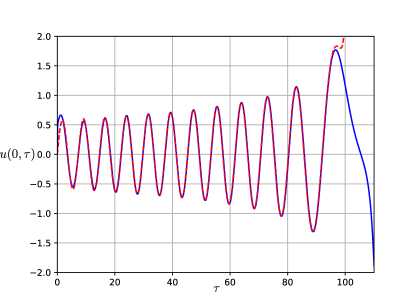
Figure 2: Comparing the analytical solution (55), (59), (62), (63) obtained for $p=\delta(\tau)$ (the red dashed line) and the numerical solution obtained for $p(\tau)=\tau_{0}^{-1}(H(\tau)-H(\tau-\tau_{0}))$ (the blue solid line) in the case $c^{2}(\epsilon\tau)={4-\epsilon\tau}$. Here $\epsilon=0.03,\ \tau_{0}=0.1$. The localized buckling occurs at $\tau=100$.

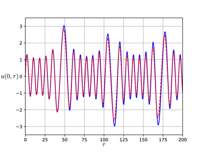
Figure 3: Comparing the analytical solution (55), (59), (62), (63) obtained for $p=\delta(\tau)$ (the red dashed line) and the numerical solution obtained for $p=\tau_{0}^{-1}(H(\tau)-H(\tau-\tau_{0}))$ (the blue solid line) in the case $c^{2}(\epsilon\tau)=2+0.9\sin(\epsilon\tau)$. Here $\epsilon=0.1,\ \tau_{0}=0.1.$

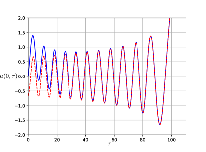
Figure 4: Comparing the analytical solution (55), (59), (60), (61), (66), (67) (the red dashed line) and the numerical solution obtained for $p=H(\tau)\exp(-\lambda\tau)$ (the blue solid line) in the case $c^{2}(\epsilon\tau)={4-\epsilon\tau}$. Here $\epsilon=0.03,\ \lambda=0.1$. The localized buckling occurs at $\tau=100$.

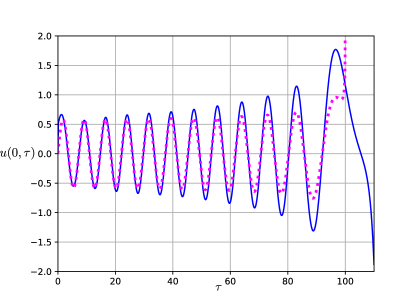
Figure 5: Comparing the approximate asymptotically incorrect analytical solution (56), (59), (68), (63) obtained for $p=\delta(\tau)$ (the magenta dotted line) and the numerical solution obtained for $p=\tau_{0}^{-1}(H(\tau)-H(\tau-\tau_{0}))$ (the blue solid line) in the case $c^{2}(\epsilon\tau)={4-\epsilon\tau}$. Here $\epsilon=0.03,\ \tau_{0}=0.1$. The localized buckling occurs at $\tau=100$.

6 Conclusion

In the paper we consider a non-stationary localized oscillations of an infinite string with slowly time-varying tension. The string lies on the Winkler foundation with a point elastic inhomogeneity (a concentrated spring with negative stiffness). We restrict ourselves to the important particular case of the general problem concerning non-stationary oscillation, where any external excitation (and, in particular, non-zero initial conditions) is applied only to the point of the string under the concentrated spring. In the case of the string with a constant tension a trapped mode of oscillations exists and is unique if and only if conditions (24), (25) are satisfied. The existence of a trapped mode leads to the possibility of the wave localization near the inhomogeneity in the Winkler foundation. Applying a vanishing as $\tau\to\infty$ external excitation to the point of the string under the inclusion leads to the emergence of undamped free oscillations localized near the spring. The most important result of the paper is analytical formulas (55), (59), (60), (61), which allow us to describe for large times such non-stationary localized oscillations in the case of slowly time-varying string tension. The obtained analytical results were verified by independent numerical calculations based on the finite difference method. The applicability of the analytical formulas was demonstrated for various types of external excitation and laws governing the varying tension (see Figures 2–4).

We also have shown that localized low-frequency oscillations with increasing amplitude precede the localized string buckling (see (56)). However, unlike the case (57) of a one degree of freedom system with time-varying stiffness, in the framework of the problem under consideration formula (56) is correct only in the limiting case, where the frequency of localized oscillations approaches zero. This fact is also verified by independent numerical calculations (see Figures 2, 5).

Finally, we note that in order to consider a more general problem, where the external excitation can be applied to an arbitrary point of the string, we need to take into account wave reflections and passing through the discrete inclusion. This makes the problem to be more sophisticated. It may be a subject of a separate future study.

Compliance with ethical standards

Conflict of Interest: The authors declare that they have no conflict of interest.

References

- (1) Ursell, F.: Trapping modes in the theory of surface waves. Mathematical Proceedings of the Cambridge Philosophical Society 47(2), 347–358 (1951)
- (2) Kaplunov, J.: The torsional oscillations of a rod on a deformable foundation under the action of a moving inertial load. Izvestiya Akademii Nauk SSSR, MTT (Mechanics of solids) 6, 174–177 (1986). (in Russian)
- (3) Abramian, A., Andreyev, V., Indeitsev, D.: The characteristics of the oscillations of dynamical systems with a load-bearing structure of infinite extent. Modelirovaniye v mekhanike 6(2), 3–12 (1992). (in Russian)
- (4) Kaplunov, J., Sorokin, S.: A simple example of a trapped mode in an unbounded waveguide. The Journal of the Acoustical Society of America 97, 3898–3899 (1995)
- (5) Abramyan, A., Indeitsev, D.: Trapping modes in a membrane with an inhomogeneity. Acoustical Physics 44, 371–376 (1998)
- (6) Gavrilov, S.: The effective mass of a point mass moving along a string on a Winkler foundation. PMM Journal of Applied Mathematics and Mechanics 70(4), 582–589 (2006)
- (7) Gavrilov, S., Indeitsev, D.: The evolution of a trapped mode of oscillations in a “string on an elastic foundation – moving inertial inclusion” system. PMM Journal of Applied Mathematics and Mechanics 66(5), 825–833 (2002)
- (8) Alekseev, V., Indeitsev, D., Mochalova, Y.: Vibration of a flexible plate in contact with the free surface of a heavy liquid. Technical Physics 47(5), 529–534 (2002)
- (9) Indeitsev, D., Osipova, E.: Localization of nonlinear waves in elastic bodies with inclusions. Acoustical Physics 50(4), 420–426 (2004)
- (10) Porter, R.: Trapped waves in thin elastic plates. Wave Motion 45(1-2), 3–15 (2007)
- (11) Kaplunov, J., Nolde, E.: An example of a quasi-trapped mode in a weakly non-linear elastic waveguide. Comptes Rendus Mécanique 336(7), 553–558 (2008)
- (12) Motygin, O.: On trapping of surface water waves by cylindrical bodies in a channel. Wave Motion 45(7-8), 940–951 (2008)
- (13) Nazarov, S.: Sufficient conditions on the existence of trapped modes in problems of the linear theory of surface waves. Journal of Mathematical Sciences 167(5), 713–725 (2010)
- (14) Pagneux, V.: Trapped modes and edge resonances in acoustics and elasticity. In: R. Craster, J. Kaplunov (eds.) Dynamic Localization Phenomena in Elasticity, Acoustics and Electromagnetism, pp. 181–223. Springer (2013)
- (15) Porter, R., Evans, D.: Trapped modes due to narrow cracks in thin simply-supported elastic plates. Wave Motion 51(3), 533–546 (2014)
- (16) Gavrilov, S., Mochalova, Y., Shishkina, E.: Trapped modes of oscillation and localized buckling of a tectonic plate as a possible reason of an earthquake. In: Proc. Int. Conf. Days on Diffraction (DD), 2016, pp. 161–165. IEEE (2016). Doi: 10.1109/DD.2016.7756834
- (17) Kaplunov, J., Rogerson, G., Tovstik, P.: Localized vibration in elastic structures with slowly varying thickness. The Quarterly Journal of Mechanics and Applied Mathematics 58(4), 645–664 (2005)
- (18) Indeitsev, D., Kuznetsov, N., Motygin, O., Mochalova, Y.: Localization of linear waves. St. Petersburg University (2007). (in Russian)
- (19) Indeitsev, D., Sergeev, A., Litvin, S.: Resonance vibrations of elastic waveguides with inertial inclusions. Technical Physics 45(8), 963–970 (2000)
- (20) Indeitsev, D., Abramyan, A., Bessonov, N., Mochalova, Y., Semenov, B.: Motion of the exfoliation boundary during localization of wave processes. Doklady Physics 57(4), 179–182 (2012)
- (21) Wang, C.: Vibration of a membrane strip with a segment of higher density: analysis of trapped modes. Meccanica 49(12), 2991–2996 (2014)
- (22) Indeitsev, D., Kuklin, T., Mochalova, Y.: Localization in a Bernoulli-Euler beam on an inhomogeneous elastic foundation. Vestnik of St. Petersburg University: Mathematics 48(1), 41–48 (2015)
- (23) Indeitsev, D., Gavrilov, S., Mochalova, Y., Shishkina, E.: Evolution of a trapped mode of oscillation in a continuous system with a concentrated inclusion of variable mass. Doklady Physics 61(12), 620–624 (2016)
- (24) Gavrilov, S., Mochalova, Y., Shishkina, E.: Evolution of a trapped mode of oscillation in a string on the Winkler foundation with point inhomogeneity. In: Proc. Int. Conf. Days on Diffraction (DD), 2017, pp. 128–133. IEEE (2017). Doi: 10.1109/DD.2017.8168010
- (25) McIver, P., McIver, M., Zhang, J.: Excitation of trapped water waves by the forced motion of structures. Journal of Fluid Mechanics 494, 141–162 (2003)
- (26) Shishkina, E., Gavrilov, S., Mochalova, Y.: Non-stationary localized oscillations of an infinite Bernoulli-Euler beam lying on the Winkler foundation with a point elastic inhomogeneity of time-varying stiffness. Journal of Sound and Vibration 440C, 174–185 (2019)
- (27) Fedoruk, M.: The saddle-point method. Nauka, Moscow (1977). (in Russian)
- (28) Nayfeh, A.: Introduction to Perturbation Techniques. Wiley & Sons (1993)
- (29) Nayfeh, A.: Perturbation methods. Weily & Sons (1973)
- (30) Gao, Q., Zhang, J., Zhang, H., Zhong, W.: The exact solutions for a point mass moving along a stretched string on a Winkler foundation. Shock and Vibration 2014(136149) (2014)
- (31) Luongo, A.: Mode localization in dynamics and buckling of linear imperfect continuous structures. Nonlinear Dynamics 25, 133–156 (2001)
- (32) Abramyan, A., Vakulenko, S.: Oscillations of a beam with a time-varying mass. Nonlinear Dynamics 63(1-2), 135–147 (2011)
- (33) Abramian, A., van Horssen, W., Vakulenko, S.: On oscillations of a beam with a small rigidity and a time-varying mass. Nonlinear Dynamics 78(1), 449–459 (2014)
- (34) Abramian, A., van Horssen, W., Vakulenko, S.: Oscillations of a string on an elastic foundation with space and time-varying rigidity. Nonlinear Dynamics 88(1), 567–580 (2017)
- (35) Vladimirov, V.: Equations of Mathematical Physics. Marcel Dekker, New York (1971)
- (36) Gavrilov, S.: Non-stationary problems in dynamics of a string on an elastic foundation subjected to a moving load. Journal of Sound and Vibration 222(3), 345–361 (1999)
- (37) Feschenko, S., Shkil, N., Nikolenko, L.: Asymptotic methods in theory of linear differential equations. NY: North-Holland (1967)
- (38) Donninger, R., Schlag, W.: Numerical study of the blowup/global existence dichotomy for the focusing cubic nonlinear Klein–Gordon equation. Nonlinearity 24(9), 2547–2562 (2011)
- (39) Strauss, W., Vazquez, L.: Numerical solution of a nonlinear Klein-Gordon equation. Journal of Computational Physics 28(2), 271–278 (1978)
- (40) Strikwerda, J.: Finite difference schemes and partial differential equations, vol. 88. SIAM (2004)
- (41) Trangenstein, J.: Numerical solution of hyperbolic partial differential equations. Cambridge University Press (2009)