Analytical and numerical study of
backreacting one-dimensional holographic superconductors
in the presence of Born-Infeld electrodynamics

Abstract

We analytically as well as numerically study the effects of Born-Infeld nonlinear electrodynamics on the properties of $(1+1)$-dimensional $s$-wave holographic superconductors. We relax the probe limit and further assume the scalar and gauge fields affect on the background spacetime. We thus explore the effects of backreaction on the condensation of the scalar hair. For the analytical method, we employ the Sturm-Liouville eigenvalue problem and for the numerical method, we employ the shooting method. We show that these methods are powerful enough to analyze the critical temperature and phase transition of the one dimensional holographic superconductor. We find out that increasing the backreaction as well as nonlinearity makes the condensation harder to form. In addition, this one-dimensional holographic superconductor faces with second order phase transition and their critical exponent has the mean field value $\beta={1}/{2}$.

I Introduction

The most well-known theory for describing the mechanism behind superconductivity from microscopic perspective is the BCS theory proposed by Bardeen, Cooper and Schrieffer. According to BCS theory, the condensation of Cooper pairs into a boson-like state, at low temperature, is responsible for infinite conductivity in solid state system BCS (1957). However, when the temperature increases, the Cooper pairs decouples and thus the BCS theory is unable to explain the mechanism of superconductivity for high temperature superconductors BCS (1957). The correspondence between gravity in an Anti de-Sitter (AdS) spacetime and a Conformal Field Theory (CFT) living on the boundary of the spacetime provides a powerful tool for calculating correlation functions in a strongly interacting field theory using a dual classical gravity description Maldacena. (1998). According to the AdS/CFT duality proposal an $n$-dimensional conformal field theory on the boundary is equivalent to gravity theory in $(n+1)$-dimensional AdS bulk Maldacena. (1998); Gubser et al. (1998); Witten et al. (1998); H08 ; Horowitz et al. (2008); Ren. (2010). The dictionary of AdS/CFT duality implies that each quantity in the bulk has a dual on the boundary. For example, energy-momentum tensor $T_{\mu\nu}$ on the boundary corresponds to the bulk metric $g_{\mu\nu}$Gubser et al. (1998); Witten et al. (1998). Based on this duality, Hartnoll et al. proposed a model for holographic superconductor in $2008$ H08 . Their motivation was to shed light on the problem of high temperature superconductors. According to the holographic superconductors, we need a hairy black hole in gravity side to describe a superconductor on its boundary. During the past decade, the investigation on the holographic superconductor has got a lot of attentions (see e.g. Horowitz et al. (2008); Ren. (2010); Hartnoll (2009); Herzog. (2009); Horowitz (2011); Gubser. (2009); HHH. (2008); Jing ,Chena (210); Salahi et al. (2016); Sheykhi et al. (2016); cai (2015); Ge (2010); SHsh (17); CAI (11); SHSH (16); shSh(16) ; Doa ; Afsoon ; cai (10, 14); yao (2013); n3 ; n4 ; n5 ; n6 ; Gan1 ).

On the other hand, BTZ (Bandos-Teitelboim-Zanelli) black holes, the well-known solutions of general relativity in $(2+1)$-dimensional spacetime, provide a simplified model to investigate some conceptual issues in black hole thermodynamics, quantum gravity, string theory, gauge theory and AdS/CFT correspondance Car1 ; Ash ; Sar ; Wit1 ; Car2 . It has been shown that the quasinormal modes in this spacetime coincide with the poles of the correlation function in the dual CFT. This gives quantitative evidence for AdS/CFT Bir . In addition, BTZ black holes play a crucial role for improving our perception of gravitational interaction in low dimensional spacetimes Wit2 . These kind solutions have been studied from different point of views rin1 ; rin2 ; rin3 ; rin4 .

Holographic superconductors dual to asymptotic BTZ black holes have been explored widely (see e.g. Wang ; chaturvedi ; Li (2012); momeni ; peng17 ; lashkari ; hua ; yanyan ; yan ; alkac ; 50-1 ; bina ). In order to construct the $(1+1)$-dimensional holographic superconductors one should employ the $AdS_{3}/CFT_{2}$ correspondence. In chaturvedi , the $(1+1)$-dimensional holographic superconductors were explored in the probe limit and its distinctive features in both normal and superconducting phases were investigated. Employing the variational method of the Sturm-Liouville eigenvalue problem, the one-dimensional holographic superconductors have been analytically studied in Li (2012); momeni ; peng17 . It is also interesting to study the $(1+1)$-dimensional holographic superconductor away from the probe limit by considering the backreaction. In Wang , the effects of backreaction have been studied for $s$-wave linearly charged one-dimensional holographic superconductors.

Holographic superconductors have also been studied extensively in the presence of nonlinear electrodynamics (see e.g. n4 ; Sheykhi et al. (2016); Salahi et al. (2016); SHsh (17); SHSH (16); shSh(16) ; n3 ; n5 ; n6 ). The most famous nonlinear electrodynamic is Born-Infeld electrodynamic. This model was presented for the first time to solve the problem of divergence of electrical field at the position of point particle 25 ; 26 ; 27 ; 28 ; 29 . It was later showed that this model could be reproduced by string theory. In the present work, we would like to extend the investigation on the $(1+1)$-dimensional holographic superconductors by taking into account the nonlinear Born-Infeld (BI) electrodynamics, as our gauge field. As well, we will study the effects of backreaction on our holographic superconductors. We perform our investigation both analytically and numerically and shall compare the result of two methods. Our analytical approach is based on the Sturm-Liouville variational method. In latter study, we find the relation between critical temperature and chemical potential. Moreover, in order to study our holographic superconductors numerically, we use the shooting method. We show that analytical results are in good agreement with numerical ones which implies that the Sturm-Liouvile variation method is still powerful enough for studying the $(1+1)$-dimensional holographic superconductor.

The structure of our paper is as follows. In section II, the basic field equations of one-dimensional holographic superconductors with backreaction in the presence of BI nonlinear electrodynamics is introduced. In section III, we describe the procedure of analytical study of one dimensional holographic superconductor based on Sturm-Liouvile method and obtain the relation between critical temperature and chemical potential. In section IV, the numerical approach toward the study of our holographic superconductors will be presented. Finally, we summarize our results in section V.

II Basic field equations

The action of three dimensional AdS gravity in the presence of a gauge and a scalar field is given by

$$S = \frac{1}{2\kappa^{2}}\int d^{3}x\sqrt{-g}\left(R+\frac{2}{l^{2}}\right)$$

$$+\int d^{3}x\sqrt{-g}\left[\mathcal{L}(\mathcal{F})-|\nabla\psi-iqA\psi|^{2}-m^{2}|\psi|^{2}\right],$$

where $m$ and $q$ shows the mass and the charge of scalar field, $\kappa^{2}={8\pi G_{3}}$ and $G_{3}$ is $3$-dimensional Newton gravitation constant. Also, $g$, $R$ and $l$ are the metric determinant, Ricci scalar and AdS radius, respectively. In (LABEL:act), $\mathcal{F}=F_{\mu\nu}F^{\mu\nu}$ where $F_{\mu\nu}=\nabla_{[\mu}A_{\nu]}$ is the electrodynamics field tensor and $A_{\mu}$ is the vector potential. $\mathcal{L}(\mathcal{F})$ stands for the Lagrangian density of BI nonlinear electrodynamics defined as

$$\mathcal{L}(\mathcal{F})=\frac{1}{b}\left(1-\sqrt{1+\frac{b\mathcal{F}}{2}}\right),$$ (2)

where $b$ is the nonlinear parameter. When $b\rightarrow 0$, $\mathcal{L}$ reduces to $-F_{\mu\nu}F^{\mu\nu}/{4}$ which is the standard Maxwell Lagrangian H08 . Variation of the above action with respect to scalar field $\psi$, gauge field $A_{\mu}$ and the metric $g_{\mu\nu}$ yield the following equations of motion

$$0 = \left(\nabla_{\mu}-i{q}A_{\mu}\right)\left(\nabla^{\mu}-i{q}A^{\mu}\right)\psi-m^{2}\psi\,,$$ (3)

$$0 = \nabla^{\mu}\left(4\mathcal{L}_{\mathcal{F}}F_{\mu\nu}\right)$$ (4)

$$-i{q}\left[-\psi^{\ast}(\nabla_{\nu}-i{q}A_{\nu})\psi+\psi(\nabla_{\nu}+i{q}A_{\nu})\psi^{\ast}\right]\,,$$

$$0 = \frac{1}{2\kappa^{2}}\left[R_{\mu\nu}-g_{\mu\nu}\left(\frac{R}{2}+\frac{1}{l^{2}}\right)\right]+2F_{ac}F_{b}{}^{c}\mathcal{L}_{\mathcal{F}}$$

$$-\frac{g_{\mu\nu}}{2}\left[\mathcal{L}(\mathcal{F})-m^{2}|\psi|^{2}-{|\nabla\psi-i{q}A\psi|^{2}}\right]$$

$$-\frac{1}{2}\left[(\nabla_{\mu}\psi-i{q}A_{\mu}\psi)(\nabla_{\nu}\psi^{\ast}+i{q}A_{\nu}\psi^{\ast})+\mu\leftrightarrow\nu\right],$$

where $\mathcal{L}_{\mathcal{F}}=\partial\mathcal{L}/\partial{\mathcal{F}}$.

Since, we would like to consider the effect of the backreaction on the holographic superconductor, we take a metric ansatz as follows Wang

$${ds}^{2}=-f(r)e^{-\chi(r)}{dt}^{2}+\frac{{dr}^{2}}{f(r)}+\frac{r^{2}}{l^{2}}{dx}^{2}.$$ (6)

The Hawking temperature of the three dimensional black hole on the outer horizon $r_{+}$ (where $r_{+}$ is the horizon radius obtained as the largest root of $f(r_{+})=0$), may be obtained through the use of the general definition of surface gravity SheyKaz

$$T = \frac{\kappa_{sg}}{2\pi}=\frac{1}{2\pi}\sqrt{-\frac{1}{2}(\nabla_{\mu}\chi_{\nu})(\nabla^{\mu}\chi^{\nu})},$$ (7)

where $\kappa_{sg}$ is the surface gravity and $\chi=\partial/\partial t$ is the null killing vector of the horizon. Taking $\chi^{\nu}=(-1,0,0)$, we have $\chi_{\nu}=(f(r_{+})e^{-\chi(r_{+})},0,0)$ and hence on the horizon where $f(r_{+})=0$, we find $(\nabla_{\mu}\chi_{\nu})(\nabla^{\mu}\chi^{\nu})=-\frac{1}{2}\left[f^{\prime}(r_{+})\right]^{2}e^{-\chi(r_{+})}$. Thus, the temperature is obtained as

$$T=\frac{e^{-\chi(r_{+})/2}f^{{}^{\prime}}(r_{+})}{4\pi}.$$ (8)

We also choose the scalar and the gauge fields as H08

$$A_{\mu}=(\phi(r),0,0),\ \ \ \psi=\psi(r).$$ (9)

Substituting (6) and (9) into the field equations (3)-(LABEL:Eein), we arrive at

$$0 = \psi^{\prime\prime}+\psi^{\prime}\left[\frac{1}{r}+\frac{f^{\prime}}{f}-\frac{\chi^{\prime}}{2}\right]+\psi\left[\frac{q^{2}\phi^{2}{\mathrm{e}}^{\chi}}{f^{2}}-\frac{m^{2}}{f}\right],$$ (10)

$$0 = \phi^{\prime\prime}+\phi^{\prime}\left[-\frac{be^{\chi}\phi^{\prime 2}}{r}+\frac{\chi^{\prime}}{2}+\frac{1}{r}\right]-\frac{2q^{2}\psi^{2}\phi}{f}\left[1-be^{\chi}\phi^{\prime 2}\right]^{3/2},$$

$$0 = f^{\prime}-\frac{2r}{l^{2}}$$

$$+2\kappa^{2}r\left[\frac{q^{2}e^{\chi}\psi^{2}\phi^{2}}{f}+f\psi^{\prime 2}+m^{2}\psi^{2}-\frac{1}{b}+\frac{1}{b\sqrt{1-be^{\chi}\phi^{\prime 2}}}\right],$$

$$0 = \chi^{\prime}+4\kappa^{2}r\left[\frac{q^{2}\phi^{2}\psi^{2}{\mathrm{e}}^{\chi}}{f^{2}}+\psi^{\prime 2}\right],$$ (13)

where the prime denotes derivative with respect to $r$. Note that in the presence of nonlinear BI electrodynamics the Eqs. (10) and (13) do not change compared to the linear Maxwell case. In the limiting case where $b\rightarrow 0$ the equations of motion (LABEL:phir) and (LABEL:fr) turn to the corresponding equations of one dimensional holographic superconductor with Maxwell field Wang . The field equations (10)-(13) enjoy the symmetries

$$q\rightarrow q/a,\text{ \ \ \ \ }\phi\rightarrow a\phi,\text{ \ \ \ \ }\psi\rightarrow a\psi,$$

$$\kappa\rightarrow\kappa/a,\text{ \ \ \ \ }b\rightarrow b/a^{2},$$ (14)

$$l\rightarrow al,\text{ \ \ \ \ }r\rightarrow ar,\text{ \ \ \ \ }q\rightarrow q/a,$$

$$m\rightarrow m/a,\text{ \ \ \ \ }b\rightarrow a^{2}b.$$ (15)

Hereafter, we set $q$ and $l$ equal to unity by virtue of these symmetries. The behavior of our model functions for large $r$ (near the boundary) read

$$\chi\rightarrow 0,\ \ \ f(r)\sim r^{2},$$

$$\phi\sim\rho+\mu\ln(r),\ \ \ \psi\sim\psi_{-}r^{-\Delta_{-}}+\psi_{+}r^{-\Delta_{+}},$$ (16)

where $\mu$ and $\rho$ are the chemical potential and the charge density of the field theory on the boundary and $\Delta_{\pm}=1\pm\sqrt{1+m^{2}}$ which implies $m^{2}\geq-1$. Actually, $\chi$ could be a constant near the boundary but by using the symmetry of field equation $\mathrm{e}^{\chi}\rightarrow a^{2}\mathrm{e}^{\chi},$ $\phi\rightarrow\phi/a$, it could be set to zero there. From holographic superconductors point of view, either $\psi_{+}$ or $\psi_{-}$ can be dual to the expectation value of condensation operator (or order operator) $\left\langle O\right\rangle$ while the other is dual to its source. We give $\psi_{-}$ the role of source and $\psi_{+}$ the role of expectation value of the order parameter $\left\langle O_{+}\right\rangle$ in this work. Since we seek for study the effects of $b$ and $\kappa$ on our holographic superconductors and different values of the scalar field mass do not influence this behavior qualitatively, we consider $m^{2}=0$ in this work. With this choice, we have $\Delta_{+}=2$, $\Delta_{-}=0$ and thus

$$\psi\sim\psi_{-}+\frac{\psi_{+}}{r^{2}},$$ (17)

near the boundary. We set $\psi_{-}=0$ at the boundary and consider $\psi_{+}$ as the dual of order parameter $\left\langle O_{+}\right\rangle$. It is remarkable to note that the asymptotic solution for $\psi$ given in Eq. (17) do not depend on the type of electrodynamics and thus for the Maxwell case in three dimensions the solution is the same as in Eq. (17). While the solution depends on the spacetime dimensions. This is due to the fact that equation for the $\psi$ given in (10) is independent on the type of electrodynamics but depends on the spacetime dimensions and the mass parameter $m$ Wang ; Doa ; ghor .

The next step is to solve the coupled nonlinear field equations (10)-(13) simultaneously and obtain the behavior of model functions. Then, we could figure out the behavior of different parameters of holographic superconductor specially the order parameter $\left\langle O_{+}\right\rangle$ and the critical temperature by using these functions. In this work, we use both analytical and numerical methods for studying the holographic superconductor. For analytical study, we perform Sturm-Liouville method while for numerical study, we use shooting method.

III Sturm-Liouville method

Table 1: Analytical results of ${T_{c}}/{\mu}$ for different values of backreaction and nonlinearity parameters.

	$b=0$		$b=0.04$		$b=0.08$
	Analytical	Numerical	Analytical	Numerical	Analytical	Numerical
$\kappa^{2}=0$	$0.0429$	$0.0460$	$0.0360$	$0.0410$	$0.0275$	$0.0362$
$\kappa^{2}=0.05$	$0.0399$	$0.0369$	$0.0337$	$0.0326$	$0.0260$	$0.0286$
$\kappa^{2}=0.1$	$0.0381$	$0.0295$	$0.0311$	$0.0260$	$0.0218$	$0.0227$
$\kappa^{2}=0.15$	$0.0352$	$0.0236$	$0.0280$	$0.0207$	$0.0174$	$0.0180$
$\kappa^{2}=0.2$	$0.0313$	$0.0189$	$0.0242$	$0.0165$	$0.0136$	$0.0143$
$\kappa^{2}=0.25$	$0.0264$	$0.0151$	$0.0195$	$0.0131$	$0.0089$	$0.0114$

In this section, we employ the Sturm-Liouville eigenvalue problem to investigate analytically the phase transition of one dimensional $s$-wave holographic superconductor in the presence of BI nonlinear electrodynamics. In addition, we calculate the relation between the critical temperature $T_{c}$, and chemical potential $\mu$, near the horizon. Furthermore, we study the effect of backreaction and BI nonlinear electrodynamics on the critical temperature. For future convenience, we define a new variable $z=r_{+}/r$ $(\in\left[0,1\right])$. With this new coordinate, the field equations (10)-(13) could be rewritten as

$$0 = \psi^{\prime\prime}+\psi^{\prime}\left[\frac{f^{\prime}}{f}-\frac{\chi^{\prime}}{2}+\frac{1}{z}\right]+\psi\left[\frac{r_{+}^{2}e^{\chi}\phi^{2}}{z^{4}f^{2}}-\frac{m^{2}r_{+}^{2}}{z^{4}f}\right],$$

$$0 = \phi^{\prime\prime}+\phi^{\prime}\left[\frac{bz^{3}e^{\chi}\phi^{\prime 2}}{r_{+}^{2}}+\frac{\chi^{\prime}}{2}+\frac{1}{z}\right]-\frac{2r_{+}^{2}\psi^{2}\phi}{z^{4}f}\Upsilon^{\frac{3}{2}},$$ (19)

$$0 = f^{\prime}+\frac{2r_{+}^{2}}{z^{3}}+\frac{2r_{+}^{2}\kappa^{2}}{z^{3}}$$

$$\times\left[\frac{1}{b}\left(1-\Upsilon^{-\frac{1}{2}}\right)-\frac{z^{4}f\psi^{\prime 2}}{r_{+}^{2}}-\frac{e^{\chi}\psi^{2}\phi^{2}}{f}-m^{2}\psi^{2}\right],$$

$$0 = \chi^{\prime}-4\kappa^{2}\left[\frac{r_{+}^{2}e^{\chi}\psi^{2}\phi^{2}}{z^{3}f^{2}}+z\psi^{\prime 2}\right],$$ (21)

where $\Upsilon=1-bz^{4}e^{\chi}\phi^{\prime 2}/r_{+}^{2}$ and now the prime indicates the derivative with respect to $z$. Since in the vicinity of critical temperature the order parameter is small, we can consider it as an expansion parameter

$$\epsilon\equiv\left\langle O_{i}\right\rangle,$$

where $i=+$ or $-$. We focus on solutions for small values of condensation parameter $\epsilon$, therefore we can expand the model functions as

$$\psi\approx\epsilon\psi_{1}+\epsilon^{3}\psi_{3}+\epsilon^{5}\psi_{5}+\cdots,$$

$$\phi\approx\phi_{0}+\epsilon^{2}\phi_{2}+\epsilon^{4}\phi_{4}+\cdots,$$

$$f\approx f_{0}+\epsilon^{2}f_{2}+\epsilon^{4}f_{4}+\cdots,$$

$$\chi\approx\epsilon^{2}\chi_{2}+\epsilon^{4}\chi_{4}+\cdots,$$

where $\epsilon\ll 1$ near the critical temperature. Moreover, by considering $\delta\mu_{2}>0$, the chemical potential can be expressed as:

$$\mu=\mu_{0}+\epsilon^{2}\delta\mu_{2}+...\rightarrow\epsilon\thickapprox\Bigg{(}\frac{\mu-\mu_{0}}{\delta\mu_{2}}\Bigg{)}^{1/2}.$$

During phase transition, $\mu_{c}=\mu_{0}$, thus the order parameter vanishes. Meanwhile, the critical exponent $\beta=\frac{1}{2}$ is in a good agreement with mean field theory result.

At zeroth order of $\epsilon$, the gauge field equation of motion (19) reduces to

$$\phi^{\prime\prime}+\frac{\phi^{\prime}}{z}+\frac{bz^{3}\phi^{\prime 3}}{r_{+}^{2}}=0,$$ (22)

which could be rewritten as a first order Bernoulli differential equation by taking $\phi^{\prime}$ as a new function TL (2000). Therefore, one receives

$$\phi^{\prime}=\frac{\lambda r_{+}}{z\sqrt{b\lambda^{2}z^{2}+1}},$$ (23)

for small values of $b$ where we define $\lambda=\mu/r_{+}$ and fix the integration constants by looking at the behavior of $\phi$ near the boundary given in (16). Integrating (23) and using the fact that $\phi(z=1)=0$, we can obtain

$$\phi_{0}(z) = \int_{1}^{z}\frac{\lambda r_{+}}{z}\left(1-\frac{1}{2}b\lambda^{2}z^{2}\right)\,dz$$ (24)

$$= \lambda r_{+}\log(z)-\frac{1}{4}b\lambda^{3}r_{+}\left(z^{2}-1\right).$$

When $b=0$ the above equation reduces to one of Li (2012). Note that at the zeroth order with respect to $\epsilon$, $\psi_{0}=\chi_{0}=0$. Substituting (23) in the (LABEL:fz), the equation for $f$ at the zeroth order with respect to $\epsilon$ has the following form

$$f_{0}(z)=r_{+}^{2}g(z),$$

$$\text{\ }g(z)=\frac{1}{z^{2}}-1+\frac{1}{8}b\kappa^{2}\lambda^{4}\left(1-z^{2}\right)+\kappa^{2}\lambda^{2}\log(z).$$ (25)

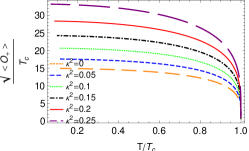
(a)  b=0

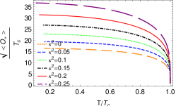
(b)  b=0.04

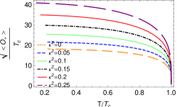
(c)  b=0.08

Figure 1: The behavior of condensation parameter as a function of temperature for different values of backreaction.

(a)  $\kappa^{2}$=0

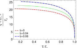
(b)  $\kappa^{2}$=0.10

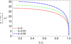
(c)  $\kappa^{2}$=0.20

Figure 2: The behavior of condensation parameter as a function of temperature for different values of nonlinearity parameter $b$.

The asymptotic behavior of the scalar field $\psi$ was given in (16). Near the boundary, we define the function $F(z)$ so that

$$\psi(z)=\frac{\left\langle O_{i}\right\rangle z^{\triangle_{i}}}{\sqrt{2}r_{+}^{\triangle_{i}}}F(z).$$ (26)

Inserting Eq. (26) in Eq. (LABEL:psiz) yields

$$F^{\prime\prime}(z)+F^{\prime}(z)\left[\frac{g^{\prime}(z)}{g(z)}+\frac{2\Delta}{z}+\frac{1}{z}\right]$$

$$+ F(z)\left[\frac{\Delta g^{\prime}(z)}{zg(z)}-\frac{m^{2}}{z^{4}g(z)}+\frac{\Delta^{2}}{z^{2}}\right]$$

$$- \frac{F(z)}{2z^{4}g(z)^{2}}\left[\lambda^{2}\log(z)\left(b\lambda^{2}r_{+}\left(z^{2}-1\right)-2\log(z)\right)\right]=0.$$

We can rewrite this equation in the Sturm-Liouville form as

$$\left[T(z)F^{\prime}(z)\right]^{\prime}+P(z)T(z)F(z)+\lambda^{2}Q(z)T(z)F(z)=0,$$ (28)

where the functions $T$, $P$, $Q$ are defined as

$$T(z)=z^{2\Delta+1}\left[\frac{1}{z^{2}}-1+\frac{1}{8}b\kappa^{2}\lambda^{4}\left(1-z^{2}\right)+\kappa^{2}\lambda^{2}\log(z)\right].$$ (29)

$$P(z)=\frac{\Delta}{z}\left(\frac{g^{\prime}(z)}{g(z)}+\frac{\Delta}{z}\right)-\frac{m^{2}}{z^{4}g(z)},$$ (30)

$$Q(z)=-\frac{\log(z)\left(b\lambda^{2}r_{+}\left(z^{2}-1\right)-2\log(z)\right)}{2z^{4}g(z)^{2}}.$$ (31)

We can consider the trial function $F(z)=1-\alpha z^{2}$ which satisfies the required boundary conditions $F(0)=1$ and $F^{{}^{\prime}}(0)=0$. Then, the eigenvalue problem could be solved for (28) by minimizing the expression

$$\lambda^{2}=\frac{\int_{0}^{1}T\left(F^{\prime 2}-PF^{2}\right)dz}{\int_{0}^{1}TQF^{2}dz},$$ (32)

with respect to $\alpha$. For backreacting parameter, we could use the iteration method and define LPJW2015

$$\kappa_{n}=n\Delta\kappa,\ \ \ n=0,1,2,\cdots,$$ (33)

where $\Delta\kappa=\kappa_{n+1}-\kappa_{n}$. Here, we take $\Delta\kappa=0.05$. Since we are interested in finding the effects of nonlinearity on backreaction up to the order $\kappa^{2}$, we have

$$\kappa^{2}\lambda^{2}={\kappa_{n}}^{2}\lambda^{2}={\kappa_{n}}^{2}(\lambda^{2}|_{\kappa_{n-1}})+O[(\Delta\kappa)^{4}],$$ (34)

where we take $\kappa_{-1}=0$ and $\lambda^{2}|_{\kappa_{-1}}=0$. We shall also retain the linear terms with respect to nonlinearity parameter $b$ and therefore,

$$b\lambda^{2}=b\left(\lambda^{2}|_{b=0}\right)+\mathcal{O}(b^{2}).$$ (35)

Then, the minimum eigenvalue of Eq. (32) can be obtained. At the critical point, temperature is defined as (see Eq. (8) and note that at zeroth order with respect to $\epsilon$, $\chi$ is zero.)

$$T_{c}=\frac{f^{\prime}\left(r_{+c}\right)}{4\pi}.$$ (36)

Using Eqs. (LABEL:fr) and (24), we receive

$$f^{\prime}\left(r_{+c}\right)=2r_{+c}+\frac{2\kappa^{2}r_{+c}}{b}\left[1-\frac{1}{\sqrt{1-b\phi^{\prime}\left(r_{+c}\right){}^{2}}}\right],$$ (37)

and thus

$$T_{c} = \frac{1}{4\pi}(\frac{\mu}{\lambda})[2-\kappa_{n}^{2}(\lambda^{2}|_{\kappa_{n-1}})$$ (38)

$$-\frac{3}{4}b\kappa_{n}^{2}(\lambda^{4}|_{\kappa_{n-1},b=0})+b\kappa_{n}^{2}(\lambda^{4}|_{\kappa_{n-1},b=0})].$$

As an example, if $b=\kappa^{2}=0$ we have

$$\lambda^{2}=\dfrac{\frac{2}{3}\alpha^{2}-\frac{4}{3}\alpha+1}{-\frac{251\alpha^{2}}{864}+\frac{9\alpha}{16}+\frac{\alpha^{2}\zeta(3)}{4}-\frac{\alpha\zeta(3)}{2}+\frac{\zeta(3)}{4}-\frac{1}{4}}.$$

Inserting $\alpha=0.759$, $\lambda_{min}^{2}=13.76$ and $T_{c}=0.429\mu$. The latter result perfectly agrees with ones in Li (2012).

The values of $T_{c}/\mu$ for different backreaction and nonlinearity parameters are listed in 1. As it shows, the effect of increasing the backreaction parameter $\kappa$ for a fixed value of nonlinearity parameter $b$ follows the same trend as raising $b$ for a fixed value of $\kappa$. In both cases, the critical temperature $T_{c}$ diminishes by growing the backreaction or nonlinearity parameters. It shows that the presence of backreaction and Born-Infeld nonlinear electrodynamics make the scalar hair harder to form. In next section, we will re-study the problem numerically using the shooting method.

IV Shooting method

In this section, we will study our holographic superconductor numerically. In order to do this, we use the shooting method Hartnoll (2009). In this method, the boundary values is found by setting appropriate initial conditions. So, for doing this, we need to know the behavior of equations of motion both at horizon and boundary. Using Taylor expansion at horizon around $z=1$, we get

$$f(z)=f_{1}\left(1-z\right)+f_{2}\left(1-z\right){}^{2}+\cdots,$$ (39)

$$\phi(z)=\phi_{1}\left(1-z\right)+\phi_{2}\left(1-z\right){}^{2}+\cdots,$$ (40)

$$\psi(z)=\psi_{0}+\psi_{1}\left(1-z\right)+\psi_{2}\left(1-z\right){}^{2}+\cdots,$$ (41)

$$\chi(z)=\chi_{0}+\chi_{1}\left(1-z\right)+\chi_{2}\left(1-z\right){}^{2}+\cdots.$$ (42)

Note that $\phi=0$ at horizon, otherwise it will be ill-defined there. In our procedure, we find all coefficients in terms of $\phi_{1}$, $\psi_{0}$ and $\chi_{0}$ by using equations of motion. Varying them at the horizon, we try to get $\psi_{-}=\chi=0$ at the boundary. So, the values of $\psi_{+}$ and $\mu$ are achieved. In addition, we will set $r_{+}=1$ by virtue of the equations of motion’s symmetry

$$r\rightarrow ar,\text{ \ \ \ \ }f\rightarrow a^{2}f,\text{ \ \ \ \ }\phi\rightarrow a\phi.$$

Performing numerical solution, we can find the values of $T_{c}/\mu$ for different backreaction and nonlinearity parameters. In order to compare the latter results with analytical ones, we listed both of them next to each other in table 1. It is obvious that there is a reasonable agreement between the results of both methods. Moreover, in table 1, the results of Wang for $b=0$ has been recovered for different values of backreaction parameter. As one could see in this table, increasing the backreaction parameter for a fixed value of $b$, decreases the critical temperature. This means that the larger values of backreaction parameter makes the condensation harder to form. Similarly, for a fixed value of $\kappa$, increasing the nonlinearity of electrodynamic model makes scalar hair harder to form because it diminishes the critical temperature.

Figs. 1 and 2 give information about the effect of backreaction and nonlinear electrodynamic on condensation. All curves follow a same trend. As $b\rightarrow 0$, we regain the results of Maxwell case presented in Wang . As figures show, the condensation gap increases by making backreaction and nonlinearity parameters larger while the other one is fixed. So, it can be understood that it is harder to form a superconductor. This is in agreement with the results obtained from the behavior of critical temperature before.

V Summary and discussion

In this work, by using the Sturm-Liouville eigenvalue problem, we analytically investigated the properties of $(1+1)$-dimensional holographic superconductor developed in BTZ black hole background in the presence of BI nonlinear electrodynamics. We have relaxed the probe limit and further assumed that the gauge and scalar fields do backreact on the background metric. We determined the critical temperature for different values of backreaction and nonlinear parameters. We have also continued our study by using the numerical shooting method and confirmed that the analytical results are in agreement with the numerical approach. We observed that the formation of the scalar hair is harder in the presence of BI nonlinear electrodynamics as well as backreaction and it becomes harder and harder to form by increasing the strength of either the nonlinear and backreaction parameters.

Finally, it would be of interest to extend this procedure for other nonlinear electrodynamics like Power-Maxwell and logarithmic cases and investigate the effects of nonlinear electrodynamics on the critical temperature and condensation operator of one dimensional holographic superconductors. These issues are now under investigations and the results will be appeared elsewhere.