Abstract

We report an exact likelihood computation for Linear Gaussian Markov processes that is more scalable than existing algorithms for complex models and sparsely sampled signals. Better scaling is achieved through elimination of repeated computations in the Kalman likelihood, and by using the diagonalized form of the state transition equation. Using this efficient computation, we study the accuracy of kernel learning using maximum likelihood and the posterior mean in a simulation experiment. The posterior mean with a reference prior is more accurate for complex models and sparse sampling. Because of its lower computation load, the maximum likelihood estimator is an attractive option for more densely sampled signals and lower order models. We confirm estimator behavior in experimental data through their application to speleothem data.

1 Introduction

Gaussian processes (GPs) are used in a wide range of applications in science and engineering Rasmussen & Williams (2006). A GP model with a fixed kernel suffices for some applications. However, typically it is required to learn the kernel from available data. Furthermore, there is a trend towards more complex kernel parametrizations beyond the basic models with a few parameter, such as the Matérn or squared exponential kernels. An example of this trend is deep kernel learning, where a neural network is used as part of the model Wilson et al. (2016). This trend agrees well with results from the domain of time series analysis, where it was found that simple models are adequate in describing some processes, but models of moderate to high complexity are typically preferred, and often critical to solve the problem at hand Prado & West (2010).

In many applications of Gaussian processes, kernel learning is performed from irregularly spaced samples, either by experimental design, e.g. in Bayesian optimization Ghahramani (2015), or as a result of the sampling process, e.g. in climate data Sinha et al. (2015) and exoplanet detection in astronomy Khan et al. (2017). While irregular sampling offers the benefit of spectral estimation beyond the average sampling frequency Broersen (2007), this type of sampling also poses challenges for the statistical accuracy of estimated kernels Broersen (2010).

Motivated by these trends and challenges, we investigate the quality of kernel learning algorithms from irregularly sampled data. Linear Gaussian Markov models are an excellent practical choice for parametrization of Gaussian processes with a one-dimensional index set (or: time series), because of their wide applicability, computational convenience, and availability of estimation algorithms Prado & West (2010); Murphy (2012); Rasmussen & Williams (2006). As motivated in section 2.2, we focus on two Markov models: the Linear-Gaussian State-Space model and the Autoregressive model.

We compare the frequentist Maximum Likelihood (ML) estimate to the Bayesian posterior mean. We do not use strong priors so that both the ML and Bayesian estimate are only based on the model structure and the data. In this way, the Bayesian estimate can be used as a direct replacement for ML where desired. However, this work is also relevant for the situation where we use stronger priors, because in this situation we still have to decide between using the more efficient posterior mode estimate versus other point estimates such as the posterior mean. This choice is analogous to the choice between the ML and posterior mean as discussed in this paper.

The benefit of the ML estimator is that it is considerably more computationally efficient than Bayesian estimates. Many theoretical results exist that show exact equivalence between ML and Bayesian point estimates with uninformative priors for certain model structures, as well as the general result that the estimates converge in the limit of large samples Bayarri & Berger (2004). Furthermore, the ML estimate, unlike the posterior mode, is independent of the chosen model parametrization, a desirable property that it shares with preferred Bayesian point estimates such as the posterior mean. However, Broersen (2010) reports that for the kernel learning problem the ML estimator can perform poorly under certain conditions, resulting in very inaccurate models, which manifests in the kernel spectrum as spurious peaks.

In an extensive simulation study, we quantify this problem under various estimation conditions, and show that the posterior mean estimate is successful in reducing the spurious peaks, resulting in more accurate models. The simulation study is a key contribution of this paper, because only a simulation study allows a meaningful comparison between the estimators. The existing asymptotic theory does not describe the significant difference in performance between the estimators that is observed in practice.

Computational complexity is a significant challenge for kernel learning and is therefore an active area of research. For example, Dong et al. (2017) reports an algorithm for an approximate likelihood computation that scales linearly with the number of observations. As reported in a early paper by Jones Jones (1980), the exact likelihood for Linear Gaussian State-Space models can be computed with the same linear scaling; this result has been used for GP kernel learning using Maximum Likelihood Sarkka et al. (2013); Gilboa et al. (2015). In many parameter estimation problems, usage of the exact likelihood as opposed to an approximation leads to more accurate and robust estimators, and is therefore preferable. For example, for the autoregressive model, the usage of the approximate likelihood can result in non-stationary models, whereas the exact ML estimator is guaranteed to result in stationary models Broersen (2006). We introduce an improvement of the exact likelihood computation that further reduces computational cost and improves scalability with model complexity.

While we focus on parameter estimation from irregularly sampled data, the presented algorithms can directly be used for the problem of missing data. The reason is that the problem of irregular sampling is addressed by rounding sampling times to a fine regular grid, effectively converting the problem into a regularly sampled signal with a large fraction of missing data.

Section 2 provides definitions of the considered models and error metric. Section 3 introduces the likelihood computation with improved scalability. 4 describes the estimators based on this likelihood computation. Crucial to the quality evaluation of the estimators, section 5 describes the simulation experiments comparing the proposed estimators. Finally, the algorithms are applied to experimental speleothem data in section 6.

2 Definitions

2.1 Process

We consider a zero mean, stationary Gaussian Markov process $y_{n}\in\mathbb{R}^{m}$ over the discrete one-dimensional index (time) variable $n\in\mathbb{Z}$. The available observations of this process are $N_{a}$ irregularly spaced observations $y_{n_{i}}$ at index $n_{i}$, taken over a measurement interval of length $N$. The set of available index values is denoted $\mathfrak{N}$. If a mean value or trend is present in a dataset, it can be subtracted as preprocessing, and be added back to the predictions made with the estimated model.

2.2 Linear Markov Models

We define two types of Linear Markov models: the linear Gaussian State-Space (LG-SS) model and the autoregressive (AR) model. Please refer to Prado & West (2010) and Broersen (2006) for some of the basic properties and results for these models that are used in the remainder of this section.

Following the notation in Murphy (2012), we write the linear Gaussian State-Space model as:

$$\begin{array}[]{lll}z_{n}&=&Az_{n-1}+\epsilon_{n}\\ y_{n}&=&Cz_{n}+\delta_{n}\end{array}$$

with state vector $z_{n}\in\mathbb{R}^{s}$, matrices $A\in\mathbb{R}^{s\times s}$ and $C\in\mathbb{R}^{m\times s}$; $\epsilon_{n}\in\mathbb{R}^{s}$ and $\delta_{n}\in\mathbb{R}^{m}$ are normally distributed, temporally uncorrelated stationary stochastic processes with covariance matrix $Q\in\mathbb{R}^{s\times s}$, and $R\in\mathbb{R}^{m\times m}$, respectively. The LG-SS model is the most general of the two models; the autoregressive model can be rewritten as an equivalent LG-SS model. Furthermore, this model is used to compute the Kalman likelihood in section 3.

The autoregressive model of order $p$ is defined by:

$$y_{n}=\sum_{i=1}^{p}a_{i}y_{n-1}+v_{n}$$

where the $a_{i}$ are referred to as prediction coefficients, and $v_{n}$is a normally distributed, temporally uncorrelated stationary stochastic process with covariance matrix $V\in R^{m\times m}$, written as $\sigma_{v}^{2}$ for $m=1$.

We will now discuss some of the many practical and theoretical motivations for the AR model. (i) Under mild conditions, a stationary Gaussian process can be approximated arbitrary well by an AR($p$) model of sufficiently high order, i.e. every process satisfying these conditions has an AR($\infty$) representation. (ii) AR models of low to moderate order $p$ are successfully used to model a wide range of processes: the AR(1) model is the discrete-time version of the Matérn-3/2 kernel or Ornstein–Uhlenbeck process used in machine learning, physics and economics; models of moderate order (5-30) are successful in an even wider range of applications, see, e.g., Zhang et al. (2017); Ramadona et al. (2016). Finally, (iii) AR models are used as the basis for a range of successful reduced statistics Moving Average (MA) and Autoregressive-Moving average (ARMA) estimators.

Conversely, Maximum Likelihood estimation for the MA and ARMA models is inaccurate even for regularly spaced observations. For ARMA models, the theoretical result explaining these problems is that the Cramèr-Rao lower bound for the estimation error for even the simplest ARMA(1,1) model is infinite. Because of the correspondence between ARMA models and LG-SS, the same issue exist for general LG-SS parameter estimation Auger-Méthé et al. (2016).

Since the AR model parameter fully characterize the Gaussian process, both the covariance function $k$, and the power spectral density $h$ can be computed from the AR model parameters. An alternative parametrization of the AR($p$) model are the partial autocorrelations $\phi_{i}$. Because the requirement of stationarity can be simply stated as $|\phi_{i}|<1$, this representation is central in AR parameter estimation. Partial autocorrelations are also defined for the vector AR process Marple (1987).

2.3 Error metric

In general, models should not be evaluated on the difference between estimated and true model parameters, because the impact of a given difference in parameter values can have a vastly different impact on model performance depending on the location in parameter space where this difference is observed. Furthermore, it precludes comparing models of a different structure. Rather, we should evaluate models by evaluating their accuracy when used for inference. We evaluate models using the model error ME Broersen (2006). We will now summarize some key results for ME as needed for this paper.

The model error ME is a normalized version of the one-step-ahead prediction error PE:

$$\mbox{ME}=N_{a}\left(\frac{\mbox{PE}}{\sigma_{v}^{2}}-1\right),$$

where PE is the expectation of the one-step-ahead prediction error of the estimated model compared to the generating process. Besides this direct time domain interpretation as normalized one-step ahead prediction error, it is asymptotically equivalent to the Spectral Distortion. This equivalence motivates reporting estimated models in the frequency domain using the log power spectral density. Furthermore, the model error is asymptotically equivalent to the Kullback-Leibler Divergence (KLD) for regularly sampled data. For regularly sampled data, the asymptotic expectation of ME for estimated models is equal to the number of estimated parameters: $\mbox{E}[\mbox{ME}]=p$.

The ME can be be computed efficiently for general ARMA (and consequently for LG-SS) models. Because of its use in our simulation study, here we report the expression for an estimated AR($p$) model $\hat{a}=(\hat{a}_{1},\hat{a}_{2},...,\hat{a}_{p})^{T}$ with respect to an AR($p)$ process with parameter vector $a$:

$$\mbox{ME}(\hat{a},a)=N_{a}(\hat{a}-a)^{T}R^{-1}(\hat{a}-a),$$ (1)

where $R\in$$\mathbb{R}^{p\times p}$ is the covariance matrix of $p$ consecutive observations of the true process $a$.

3 Scalable exact likelihood computation

In this section we develop a scalable exact computation of the likelihood for the LG-SS model that is more computationally efficient than the existing Kalman likelihood. This computation is used in the estimation algorithms described in section 4.

3.1 Existing methods

The likelihood for observations $y\in\mathbb{R}^{N_{a}}$, $y=(\begin{array}[]{cccc}y_{n_{1}}&y_{n_{2}}&\cdots&y_{n_{Na}}\end{array})^{T}$ of a Gaussian Process can be written as Murphy (2012):

$$L(y)=\mbox{$\mathcal{\log N}(0,K)$=}-\frac{1}{2}\log\left|K\right|-\frac{1}{2}y^{T}K^{-1}y+\mbox{constant}$$

where $\mathcal{N}(\mu,S)$ is the multivariate Gaussian distribution, and $K\in\mathbb{R}^{N_{a}\times N_{a}}$ is the data covariance matrix: $K_{ij}=k(n_{i}-n_{j})$. We refer to this computation of the likelihood for general covariance matrices $K$ as the covariance matrix (COVM) method. This method is computationally expensive, i.e. $\mathcal{O}(N_{a}^{3})$, and consequently its application is limited to small datasets.

The Kalman likelihood (KAL) is a more efficient, exact likelihood computation for LG-SS models, which uses the decomposition of the likelihood into a sum of conditional likelihoods Murphy (2012):

$$L(y)=\sum_{n\in\mathfrak{N}}\log\mathcal{N}(y_{n};\mu_{n},\Sigma_{n})$$ (2)

where the mean vector $\mu_{n}\in\mathbb{R}^{s}$ and covariance matrix $\Sigma_{n}\in\mathbb{R}^{s\times s}$ are computed using the Kalman measurement equations for each $n\in\mathfrak{N}$, while the Kalman prediction step is performed for all $N$ grid points. The Kalman likelihood for the initial state distribution is given by the Lyapunov equation. This computation is $\mathcal{O}(N)$. Since it is often beneficial to use a small grid time $T_{g}$, it is typical that $N_{a}\ll N$. Hence, we proceed to improve algorithm efficiency to achieve an exact computation of $\mathcal{O}(N_{a})$.

3.2 Kalman likelihood with precomputation

For sparsely sampled data, it will occur frequently that no data is available for several consecutive sample points. For the likelihood computation, this results in repeated application of the Kalman prediction step. In this section, we describe an algorithm that precomputes elements of the repeated prediction step, thus reducing the overall computational complexity of the likelihood computation.

Performing $k$ prediction steps in absence of measurements yields:

$$\begin{array}[]{lll}\mu_{n+k|n}&=&A^{k}\mu_{n}\\ \Sigma_{n+k|n}&=&F(A,\Sigma_{n},k)+G(A,Q,k)\end{array}$$ (3)

where $\Sigma_{n}$ is the state covariance matrix conditional on all available preceding observations, and

$$F(A,\Sigma_{n},k) =A^{k}\Sigma_{n}(A^{k})^{T}$$

$$G(A,Q,k) =\sum_{i=0}^{k-1}A^{i}Q(A^{i})^{T}$$

Computation of each of these contributions can be accelerated using precomputation of components that only depend on the model parameters, i.e. $A^{k}$ and $G(A,Q,k)$. We write $G$ in terms of the contributions to the sum: $G=\sum_{i=0}^{k-1}g_{i}$, with $g_{i}=A^{i}QA^{iT}$. For efficient computation of $g_{i}$ we use the recursive relations $g_{i}=Ag_{i-1}A^{T}$ and $G(A,Q,k)=G(A,Q,k-1)+g_{k-1}$.

After completion of the precomputation, we perform $N_{a}$ repeated prediction steps and measurement steps, each of which has constant complexity for constant $s$. Therefore, the computational complexity has been reduced to $\mathcal{O}(N_{a})$. For AR models, the computation can be further accelerated by exploiting the sparsity in $C$ and $Q$.

3.3 Diagonalized Kalman likelihood with precomputation

For more efficient computation of the matrix powers in the Kalman likelihood for larger state dimension $s$, we decompose the state vector $z$ according to the eigenbasis of $A$, yielding the following equations for the state-space model:

$$z_{n}^{e} = \Lambda z_{n-1}^{e}+\epsilon_{n}^{e}$$

$$y_{n} = C^{e}z_{n}^{e}+\delta_{n}$$

where $z^{e},\epsilon^{e}$ and $C^{e}$ are the state, process noise and $C$ matrix, expressed on eigenbasis of $A$.

This decomposition requires that $A$ is diagonalizable. The $A$ matrix corresponding to an AR($p$) model is diagonalizable as long as $a_{p}\neq 0$. If $a_{p}=0$, we can remove trailing zero-valued coefficients to obtain an AR($p^{*}$) model with $p^{*}<p$, and $a_{p}^{*}\neq 0$ which can be diagonalized. This model order reduction order does not affect the covariance function of $y$ and will therefore yield the correct likelihood value.

The measurement step is the same as in the original Kalman likelihood (KAL). The repeated prediction step (eq. 3) becomes:

$$\begin{array}[]{lll}\mu_{n+k|n}^{e}&=&\Lambda^{k}\mu_{n}^{e}\\ \Sigma_{n+k|n}^{e}&=&\Lambda^{k}\Sigma_{n}\Lambda^{kH}+\sigma_{\epsilon}^{2}\sum_{i=0}^{k-1}\Lambda^{i}Q^{e}\Lambda^{iH}\end{array}$$

which is more computationally efficient to evaluate, because $\Lambda$ is diagonal. For the functions $F$ and $G,$ we find:

$$F(\Lambda,\Sigma_{n},k)=F_{p}(\Lambda,k)\circ\Sigma_{n}$$

where $\circ$ is the elementwise matrix product or Hadamard product, and $F_{p}(\Lambda,k)[i,j]=(\lambda_{i}\lambda_{j}^{*})^{s}$. Since $F_{p}$ is data-independent, it can be precomputed. For the second contribution $G$, we find:

$$G(\Lambda,Q^{e},k)=G_{p}(\Lambda,k)\circ Q^{e}$$ (4)

with

$$G(\Lambda,k)[i,j]=\frac{1-(\lambda_{i}\lambda_{j}^{*})^{k}}{1-\lambda_{i}\lambda_{j}^{*}}$$

Equation 4 has reduced computational complexity compared to the original expression because (i) it uses the elementwise product, which is $\mathcal{O}(s^{2})$, whereas the matrix multiplication is $\mathcal{O}(s^{3})$ and (ii) the usage of the geometric series allows for efficient exponentiation, e.g. exponentiation by squaring.

Finally, the convariance of the unconditional distribution can also be computed more efficiently, because the Lyapunov equation reduces to a per-element expression:

$$\Sigma_{1|0}[i,j]=\frac{Q^{e}[i,j]}{1-\lambda_{i}\lambda_{j}^{*}}.$$

3.4 Computational load

The computational load of the likelihood computation is measured experimentally on speech sample data from Wilson & Nickisch (2015). Irregularly sampled data is derived by random subsampling. In figure 1, we report the computational load of the described likelihood computations implemented in Julia 0.6.0, and executed on a 2.60 GHz Intel Xeon E5-2670 CPU.

The experiments confirm the expected scaling behavior: Kalman-based computations scale much better with signal duration $N$ (fig.1a); precomputation methods PRE-KAL and DIAG-PRE-KAL are more efficient for larger sampling intervals compared to the original Kalman likelihood KAL (fig. 1b). Finally, the usage of the diagonalized state-space formulation (DIAG-PRE-KAL) scales better with increasing model complexity (fig. 1c). However, because PRE-KAL uses only real-valued variables, it has a lower memory footprint, which makes it more efficient for low-complexity models.

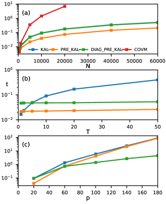
Figure 1: Execution time in seconds for likelihood computation methods as a function of the signal duration (a); average sampling interval (b) and model complexity (c).

4 Estimators

In this section we describe our implementation of the maximum likelihood and Bayesian point estimators for kernel learning for the autoregressive (AR) model. We use the PRE-KAL algorithm, which is the most efficient for the considered model complexity, implemented in the probabilistic programming language Stan Carpenter et al. (2016). The Stan script is provided as supplementary material with this paper.

4.1 Setting grid and analysis time scales

In case observations are made on a continuous index variable $t$, the time indices are converted to integer indices $n_{i}$ by rounding the continuous index variable to values on a regularly spaced grid with spacing $T_{g}$. A coarser grid will result into larger errors in the estimated process parameters. Considerations in setting this value include (i) the time scale of interest (ii) process dynamics and (iii) computational load and numerical stability.

An effective way to achieve accurate models at the time scale of interest $T_{A}$ is to simply set the grid spacing $T_{g}$ equal to $T_{A}$. However, this does not fully exploit all available data, and may introduce errors in the process dynamics that are too large. In this case, we can use modeling at interval $T_{A}$ De Waele & Broersen (2000). The discrete-time signal can be split in $T_{A}/T_{g}$ segments of data that can be treated independently, which means that the likelihood can be computed as the sum of the likelihood per segment.

4.2 Maximum Likelihood (ML) Estimator

Maximization of the likelihood is performed over the partial autocorrelations $\phi$ using the L-BFGS algorithm, initiated from a number of different starting points to reduce the probability of finding a local optimum. Three starting points are obtained using the Burg AR parameter estimator applied to regularly sampled signals derived from the original data (i) using Nearest Neighbor interpolation (ii) using Linear Interpolation and (iii) by ignoring missing data. Finally, (iv) the white noise model, i.e. $\phi_{i}=0$ for $i\in[1,p]$, is used as a starting point. The starting point resulting in the highest likelihood is used as the final estimate.

4.3 Bayesian point estimate with uninformative prior (PMEAN)

In addition to the ML estimate, we propose a Bayesian point estimate for the model parameters. While it is possible and perfectly valid to use the generated parameter samples for further inference, we use a spoint estimate here because of the following reasons: (i) In practice a posterior is rarely the end result of the analysis. Rather, the samples are used to draw a conclusion that can be formulated as a Bayesian decision problem. A point estimate can also be interpreted as a result of a decision problem Gelman et al. (2014); (ii) the point estimate allows a direct comparison with the ML estimator, and can be used as a direct replacement for it. Finally (iii) usage of a point estimate greatly reduces the computational complexity of subsequent application of the estimated kernel parameters, e.g. prediction, optimization or interpolation.

We approximate an uninformative prior by application of the AR(1) reference prior Berger & Yang (1994) to the partial autocorrelations $\phi_{i}$: $p(\phi_{i})\propto(1-\phi_{i}^{2})^{-1/2}$. The approximate location parametrization is given by $\kappa_{i}=\arcsin\phi_{i},\;-\pi<\kappa_{i}<\pi$. By definition, this is the parametrization where the reference prior is uniform Bernardo (2005).

For many estimation problems, asymptotical theory accurately describes estimator performance. In this regime, the posterior is narrow, and various point estimators converge to the same estimate, including the posterior mode, posterior mean, and the ML estimate Gelman et al. (2014). Notably, because in the asymptotic regime $\mbox{E}[f(\theta)]\approx f(\mbox{E}[\theta])$, the posterior mean of different parameterizations are equivalent. However, for irregularly sampled data, we are typically not in this regime and therefore have to be more precise in defining a Bayesian point estimate. Because the model error ME (eq. 1) is approximately quadratic in the prediction parameters $\hat{a}$, we use the posterior mean of $\hat{a}$ as point estimate: $\hat{a}=\mbox{E}[a|y]$, which is the optimal Bayesian decision for a quadratic loss in $\hat{a}$. This estimator is referred to as PMEAN. Posterior samples are drawn with the Stan implementation of Hamiltonian Monte Carlo (HMC), initiated from the ML estimate.

5 Simulation study

Simulation experiments are critical for performance evaluation of kernel learning algorithms, because the asymptotic results that can be obtained theoretically are quite different from estimator performance in practice. In section 5.1, we quantify the impact on the model error of the occurrence of spurious spectral peaks. In section 5.2, we determine the dependence of the model error on various process and model parameters.

5.1 Case study various kernels

The case study kernels are defined as follows:

• case A : exponential kernel with covariance function $\rho(r)=\exp(-r/200)$ , or, equivalently, an AR(1) process with parameter $\phi_{1}=a_{1}=\exp(-1/200)$;

• case B : squared exponential kernel with covariance function $\rho(r)=\exp(-r^{2}/10^{2})$

• case C : AR(4) process with poles $\exp(-0.02\pm 0.05\cdot 2\pi i)$, $\exp(-0.10\pm 0.30\cdot 2\pi i)$, corresponding to spectral peaks at $f=0.05$ and $f=0.30$.

Repeated irregular samples are drawn from this process as follows: (i) a random draw of $N$ observations of the process is generated from the prescribed covariance; (ii) samples are random selected selected with probability $1/T$, where $T$ is the average sampling interval. We use $N=1000$ and $T=5.$ Parameters are estimated for the AR($8$) model for case A and B, and an AR($4$) model for case C. The motivation for the lower order for case C is to create a best scenario case for the ML estimator, by matching the estimated model order with the actual model order. For the ML estimator, the ME increases more strongly with increasing model order compared to PMEAN.

The average model error over $S=400$ simulation runs is given in figure 2. We draw the following main conclusions from this experiment: (i) The Bayesian PMEAN estimator significantly reduces the model error compared to ML for case A and B. The ME is reduced by a factor of 8.2 for case A, by a factor of 3.6 for case B; (ii) All estimators perform well for case C, which shows that PMEAN is successful at suppression of spurious peaks in cases A and B, while at the same time it correctly estimates a peak when it occurs in the true spectrum.

In addition to PMEAN, we also report the results for the posterior mean with a flat prior on the partial autocorrelations $\phi_{i}$ (PMEAN-f). The results for PMEAN-f are comparable to those of PMEAN, showing that results are not sensitive to the kind of uninformative prior used. Since this result holds equally for other reported simulation experiments, PMEAN-f is not reported separately elsewhere.

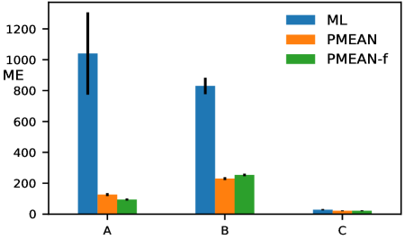
Figure 2: Model Error ME for the kernel case studies for the ML and PMEAN estimators. The posterior mean estimator PMEAN achieves a significant error reduction for cases A and B. The ME is the average over 400 simulations.

Spectral estimates for representative simulation draws are given in figure 3 in comparison to the true spectrum along with the resulting model error ME. For case A, the spectral estimate at higher frequencies for ML estimate has an error of close to 3 orders of magnitude, resulting in a large ME of 1045, while PMEAN is much more accurate in this frequency range. Also for case B, we observe that PMEAN is successful at suppression of spurious peaks compared to ML. Finally, both estimators accurately model the true spectral peak when it occurs in the true spectrum in case C.

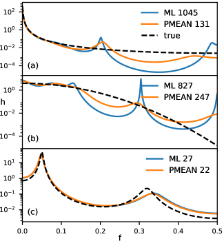
Figure 3: Estimated power spectra for representative simulation runs for the kernel case studies, compared to the true kernel spectrum. The legend shows the model error ME for each estimate.

Figure 4 shows the posterior distribution and point estimates for AR parameters $a_{1}$ through $a_{4}$ for an estimated AR(8) model for case A. Higher order coefficients are omitted because they show a similar pattern. The posterior for the (non-zero) parameter $a_{1}$ is quite narrow. Both the ML and PMEAN estimates are accurate for this parameter. However, we observe a wide posterior for the higher order coefficients, roughly centered around the true value of $0$. For these coefficients, the posterior mean, being the center of mass of the distribution, more robustly estimates a value closer to $0$ because it takes into account the entire distribution, thus resulting in a more accurate model. Conversely, the maximum likelihood estimator does not take into asccount the entire shape of the distribution, but only the maximum, and thus is more prone to shift dramatically due to small random variations, resulting in a larger error.

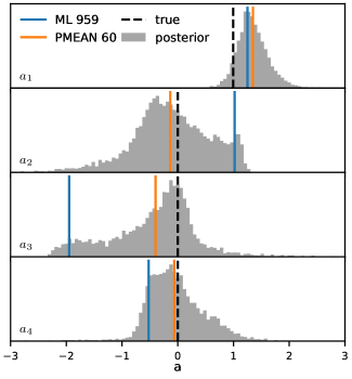
Figure 4: Posterior distribution and point estimates for AR parameters $a_{1}$ to $a_{4}$ (top to bottom) for an estimated AR(8) model for case A. The legend shows the model error ME for each estimate.

For AR(8) model estimation in cases A and B, the average computation time for the ML estimator is $2.3$ seconds, while PMEAN takes $230$ seconds. Hence, ML is the best option kernel learning when its speed is required. However, the computation time for PMEAN is reasonable and its significantly greater accuracy makes it the algorithm of choice in case the computational resources are available. Furthermore, our results can motivate future work by accelerating the sampling, e.g. by a specialized derivative computation instead of relying on the Stan autodiff algorithm; usage of the DIAG-PRE-KAL algorithm; and faster sampling algorithms such as variational inference.

5.2 Performance under range of process parameters

We report the results of a simulation experiment for a range of process parameters, using case A from section 5.1 as a reference. When varying the sampling interval $T_{s}$, the measurement time is increased in proportion to $T_{s}$ so that the average number of available samples $N_{a}$ remains constant. The results are given in figure 5

Figure 5a) shows that the ML estimator has a larger model error with increasing correlation length $T_{s}$, corresponding to a larger dynamic range in the frequency domain; increasing average sampling time $T$ (5b); and increasing estimated model order $p_{est}$ (5c).

Conversely, the model error decreases with increasing measurement time $N_{a}$ (5d), indicating that the estimator converges to an accurate result as the number of observations increases. Note that the model error is scaled with $N_{a}$. Hence, the unscaled error decreases faster than $1/N_{a}$. This is caused by finite sample effects, which are not described by asymptotic theory. In the asymptotic regime, the model error is independent of $N_{a}$.

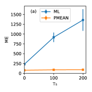
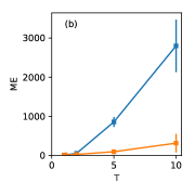
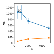
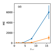
Figure 5: Model error ME of ML and PMEAN estimators as a function of correlation length $T_{s}$ (a); average sampling time $T$ (b); measurement time $N$ (c); and model order $p_{est}$(d).

6 Monsoon rainfall variability data

We investigate long-term monsoon rainfall variability based on radiometric-dated, speleothem oxygen isotope $\delta^{18}O$ data Sinha et al. (2015). This data enables evaluation of climate variability on a much larger time scale than the few decades of precipitation recorded by meteorologists. The data is intrinsically irregularly sampled, because it is formed by natural deposition rather than experimenter controlled sampling. For the same reason, irregular sampling occurs for many other long-term climate records as well, e.g. ice core data Petit et al. (1999).

Speleothem (cave formation) data as studied across various locations can have a range of average sampling rates. The current dataset is particularly suitable for algorithm benchmarking because it has a higher average sampling rate than datasets collected from other locations. This allows us to study algorithm performance as a function of sampling rate by subsampling the original data, and comparing the results to estimates obtained from the full dataset.

The oxygen isotope data consists of $N=1848$ irregularly sampled observations of $\delta^{18}O$ anomalies over a time span of $2147$ years, resulting in average sampling interval of $T_{0}=1.16$ years. We convert the irregularly sampled data to a regularly sampled grid with missing data with a grid spacing of $T_{g}=2$ years and use this data to estimate AR(8) models. Because of the high sampling rate and selected grid spacing, on 13% of samples on the regular grid are missing when all samples are used, and we can consequently estimate a reliable reference model. This is confirmed by the fact that both the ML and PMEAN are practically identical, with $\mbox{ME}<1$ between the two estimates.

We proceed to increase the average sampling interval $T$ by random subsampling to create lower-fidelity datasets as they may be observed at other locations. The sampling interval $T$ is expressed in grid time steps, so that $T=1$ corresponds to no missing data, as in the simulation experiments.

For each subsampling rate, we generate $20$ different signals by repeated random subsampling. The error of estimated AR($8$) models compared to the reference model as a function of $T$, as well as estimated power spectra for $T=6.6$ are given in figure 6.

Consistent with the simulation results, we observe that both estimators are accurate for low $T$, but that the PMEAN estimator has a substantially lower error as $T$ increases. Also, PMEAN successfully suppresses the spurious peaks at higher frequencies.

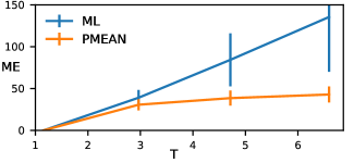
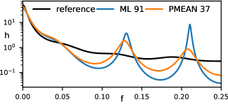
Figure 6: Estimator performance on randomly subsampled speleothem $\delta^{18}O$ data. As shown by the model error ME as a function of average sampling interval $T$ (a), the posterior mean PMEAN is substantially more accurate than ML with increasing $T$. As in the simulation experiments, the ML estimate shows spurious peaks which are strongly reduced in the PMEAN estimate (b), resulting in a lower ME (37 vs 91)

7 Concluding remarks

The reported algorithms and results are directly relevant to kernel learning when using Linear Gaussian Markov models for scalar index variables or time series. Furthermore, the results can guide a wide range of related research, as we motivate below.

First, we report that the posterior mean based on the reference prior yields considerably more accurate models than the ML estimate, which strongly deteriorates for complex models. It is expected that this result will generalize to other kernels. Considering the trend towards more complex models, this is a key result for the field of kernel learning.

Second, the Linear Gaussian Markov model can be used to model data with multidimensional index variables by using it to compose a separable multidimensional covariance function Gilboa et al. (2015).

References

- Auger-Méthé et al. (2016) Auger-Méthé, M., Field, C., Albertsen, C. M., Derocher, A. E., Lewis, M. A., Jonsen, I. D., and Flemming, J. M. State-space models’ dirty little secrets: even simple linear gaussian models can have estimation problems. Scientific reports, 6:26677, 2016.
- Bayarri & Berger (2004) Bayarri, M.J. and Berger, J. O. The interplay of Bayesian and frequentist analysis. Statistical Science, pp. 58–80, 2004.
- Berger & Yang (1994) Berger, J. O. and Yang, R.-Y. Noninformative priors and bayesian testing for the ar (1) model. Econometric Theory, 10(3-4):461–482, 1994.
- Bernardo (2005) Bernardo, J. M. Reference analysis. Handbook of statistics, 25:17–90, 2005.
- Broersen (2006) Broersen, P. M. T. Automatic autocorrelation and spectral analysis. Springer Science & Business Media, 2006.
- Broersen (2007) Broersen, P. M. T. Spectral estimation from irregularly sampled data for frequencies far above the mean data rate. In 2007 IEEE Instrumentation Measurement Technology Conference IMTC 2007, pp. 1–6, May 2007. doi: 10.1109/IMTC.2007.379314.
- Broersen (2010) Broersen, P. M. T. The removal of spurious spectral peaks from autoregressive models for irregularly sampled data. IEEE Transactions on Instrumentation and Measurement, 59(1):205–214, Jan 2010. ISSN 0018-9456. doi: 10.1109/TIM.2009.2022451.
- Carpenter et al. (2016) Carpenter, B., Gelman, A., Hoffman, M., et al. Stan: A probabilistic programming language. J Stat Softw, 2016.
- De Waele & Broersen (2000) De Waele, S. and Broersen, P. M. T. Order selection for the multirate burg algorithm. In Signal Processing Conference, 2000 10th European, pp. 1–4. IEEE, 2000.
- Dong et al. (2017) Dong, K., Eriksson, D., Nickisch, H., Bindel, D., and Wilson, A. G. Scalable log determinants for gaussian process kernel learning. In Advances in Neural Information Processing Systems, pp. 6330–6340, 2017.
- Gelman et al. (2014) Gelman, A., Carlin, J. B., Stern, H. S., and Rubin, D. B. Bayesian data analysis, volume 2. Chapman & Hall/CRC Boca Raton, FL, USA, 2014.
- Ghahramani (2015) Ghahramani, Z. Probabilistic machine learning and artificial intelligence. Nature, 521(7553):452–459, 2015.
- Gilboa et al. (2015) Gilboa, E., Saatçi, Y., and Cunningham, J. P. Scaling multidimensional inference for structured gaussian processes. IEEE transactions on pattern analysis and machine intelligence, 37(2):424–436, 2015.
- Jones (1980) Jones, R. H. Maximum likelihood fitting of arma models to time series with missing observations. Technometrics, 22(3):389–395, 1980.
- Khan et al. (2017) Khan, M. S., Jenkins, J., and Yoma, N. B. Discovering new worlds: A review of signal processing methods for detecting exoplanets from astronomical radial velocity data [applications corner]. IEEE Signal Processing Magazine, 34(1):104–115, 2017.
- Marple (1987) Marple, S. L. Digital spectral analysis: with applications, volume 5. Prentice-Hall Englewood Cliffs, NJ, 1987.
- Murphy (2012) Murphy, K. P. Machine learning: a probabilistic perspective. MIT press, 2012.
- Petit et al. (1999) Petit, J.-R., Jouzel, J., Raynaud, D., Barkov, N. I., et al. Climate and atmospheric history of the past 420,000 years from the vostok ice core, antarctica. Nature, 399(6735):429–436, 1999.
- Prado & West (2010) Prado, R. and West, M. Time series: modeling, computation, and inference. CRC Press, 2010.
- Ramadona et al. (2016) Ramadona, A. L., Lazuardi, L., Hii, Y. L., et al. Prediction of dengue outbreaks based on disease surveillance and meteorological data. PloS one, 11(3):e0152688, 2016.
- Rasmussen & Williams (2006) Rasmussen, C. E. and Williams, C. K. I. Gaussian processes for machine learning, volume 1. MIT press Cambridge, 2006.
- Sarkka et al. (2013) Sarkka, S., Solin, A., and Hartikainen, J. Spatiotemporal learning via infinite-dimensional bayesian filtering and smoothing: A look at gaussian process regression through kalman filtering. IEEE Signal Processing Magazine, 30(4):51–61, 2013.
- Sinha et al. (2015) Sinha, A., Kathayat, G., Cheng, H., et al. Trends and oscillations in the indian summer monsoon rainfall over the last two millennia. Nature communications, 6, 2015.
- Wilson & Nickisch (2015) Wilson, A. G. and Nickisch, H. Kernel interpolation for scalable structured gaussian processes (kiss-gp). In International Conference on Machine Learning, pp. 1775–1784, 2015.
- Wilson et al. (2016) Wilson, A. .G., Hu, Z., Salakhutdinov, R., and Xing, E. P. Deep kernel learning. In Artificial Intelligence and Statistics, pp. 370–378, 2016.
- Zhang et al. (2017) Zhang, Y., Liu, B., Ji, X., and Huang, D. Classification of EEG signals based on autoregressive model and wavelet packet decomposition. Neural Processing Letters, 45(2):365–378, 2017.