The fraction of ionizing radiation from massive stars that escapes to the intergalactic medium

Abstract

The part played by stars in the ionization of the intergalactic medium (IGM) remains an open question. A key issue is the proportion of the stellar ionizing radiation that escapes the galaxies in which it is produced. Spectroscopy of gamma-ray burst (GRB) afterglows can be used to determine the neutral hydrogen column-density, ${N_{{\text{H\,{i}}}}}$, in their host galaxies and hence the opacity to extreme ultra-violet (EUV) radiation along the lines-of-sight to the bursts. Thus, making the reasonable assumption that long-duration GRB locations are representative of the sites of massive stars that dominate EUV production, one can calculate an average escape fraction of ionizing radiation in a way that is independent of galaxy size, luminosity or underlying spectrum. Here we present a sample of ${N_{{\text{H\,{i}}}}}$ measures for 138 GRBs in the range $1.6<z<6.7$ and use it to establish an average escape fraction at the Lyman limit of ${\langle{f_{\rm esc}}\rangle}\approx 0.005$, with a 98% confidence upper limit of ${\langle{f_{\rm esc}}\rangle}\approx 0.015$. This analysis suggests that stars provide a small contribution to the ionizing radiation budget of the IGM at $z<5$, where the bulk of the bursts lie. At higher redshifts, $z>5$, firm conclusions are limited by the small size of the GRB sample (7/138), but any decline in average H i column-density seems to be modest. We also find no indication of a significant correlation of ${N_{{\text{H\,{i}}}}}$ with galaxy UV luminosity or host stellar mass, for the subset of events for which these are available. We discuss in some detail a number of selection effects and potential biases. Drawing on a range of evidence we argue that such effects, while not negligible, are unlikely to produce systematic errors (in either direction) of more than a factor $\sim 2$ in $f_{\rm esc}$, and so would not affect the primary conclusions. Given that many GRB hosts are low metallicity, high specific star-formation rate, dwarf galaxies, these results present a particular problem for the hypothesis that such galaxies dominated the reionization of the universe.

1 Introduction

A key question for our understanding of the reionization of hydrogen in the intergalactic medium (IGM) is the extent to which ionizing extreme ultraviolet (EUV) radiation from massive stars escapes from the galaxies in which it is produced. This can be parameterised by the escape fraction, $f_{\rm esc}$, the proportion of photons produced by stars at the Lyman limit wavelength ($\lambda=912$ Å) that leave the virial radius of their host galaxy. Only if the average escape fraction, $\langle{f_{\rm esc}}\rangle$, is sufficiently high in the era of reionization (EoR; $7\lesssim z\lesssim 9$; Planck Collaboration et al., 2016), i.e. $\langle{f_{\rm esc}}\rangle$ at least 0.1–0.2, is it likely that this phase change was predominantly driven by EUV star-light (e.g. Ouchi et al., 2009; Bouwens et al., 2012; Finkelstein et al., 2012; Robertson et al., 2015; Faisst, 2016). Otherwise some other significant source of ionizing radiation is required, such as a large population of faint quasars (Madau & Haardt, 2015; Khaire et al., 2016, but see Hassan et al. (2018) for counter arguments), X-ray binaries (Mirabel et al., 2011; Fragos et al., 2013; Knevitt et al., 2014; Madau & Fragos, 2017) or decaying/annihilating particles (Sciama, 1982; Hansen & Haiman, 2004).

Direct searches for Lyman continuum emission below 912 Å in the rest frame are compromised by absorption due to neutral gas in the intergalactic medium (the Ly$\alpha$ forest), and essentially impossible above $z\sim 4$ as the IGM absorption becomes near total – the so-called Gunn-Peterson trough (Gunn & Peterson, 1965). Observations at lower redshifts are still difficult, and there have been extensive efforts searching for such continuum emission from star-forming galaxies at $z=2$–4 in recent years (e.g Steidel et al., 2001; Shapley et al., 2006; Vanzella et al., 2010, 2012; Nestor et al., 2013; Mostardi et al., 2013; Vanzella et al., 2015; Japelj et al., 2017; Marchi et al., 2017). Results have been conflicting, particularly due to rare cases of low redshift galaxies aligning by chance with higher redshift targets (e.g. Vanzella et al., 2012; Siana et al., 2015), but given the scarcity of high escape fraction systems it appears that $f_{\rm esc}$ is not high on average (Grazian et al., 2017; Rutkowski et al., 2017). This is consistent with quasars being the primary source of EUV radiation maintaining a reionized IGM at $z<4$. However, at least some individual cases at $z\gtrsim 3$ appear to have very high escape fractions ${{f_{\rm esc}}}\gtrsim 0.5$ (de Barros et al., 2016; Vanzella et al., 2016; Shapley et al., 2016), and so might be analogues of galaxies in the EoR.

To account for the discrepancy between the expected and observed level of the escape fraction, it has been often suggested that $\langle{f_{\rm esc}}\rangle$ may actually increase with decreasing galaxy luminosity and/or with increasing redshift (e.g. Razoumov & Sommer-Larsen, 2010; Ciardi et al., 2012; Kuhlen & Faucher-Giguère, 2012; Fontanot et al., 2014; Xu et al., 2016a; Anderson et al., 2017). Observationally, it is hard to reach sufficiently stringent constraints on the escape fraction for faint galaxy populations to investigate its dependence on luminosity (e.g. Japelj et al., 2017), while due to IGM absorption the claim of a changing escape fraction with redshift can only be investigated through secondary means and simulations (e.g. Zackrisson et al., 2013; Sharma et al., 2016). The challenge facing simulators is to model in sufficient detail the complex baryonic physics and radiative transfer given limited resolution, while also sampling a range of galaxies and environments. Typically, models of an instantaneous burst of star formation incorporating only single-star stellar evolution produce the large bulk of their EUV within a few Myr, limiting the time available for feedback from winds, radiation and supernovae to open windows in the surrounding high density gas. Recently, models which include binary stellar evolution have been shown to prolong the period of high EUV production to $\sim 10$ Myr, and hence hold more promise for clearing of local gas, and for at least a relatively high fraction of stars leaving the immediate environment in which they formed (Stanway et al., 2016; Ma et al., 2016).

An alternative route, first proposed by Chen et al. (2007), to constraining $\langle{f_{\rm esc}}\rangle$ empirically over a broad range in redshift is via spectroscopy of long-duration gamma-ray burst (GRB) afterglows. These very bright, but short-lived, continuum sources allow detailed abundance studies of host galaxy gas along the line of sight. Crucially, this includes calculation of the neutral hydrogen column-density, ${N_{{\text{H\,{i}}}}}$, in the host from fitting the Ly$\alpha$ absorption feature when it is seen (e.g. Prochaska et al., 2007; Fynbo et al., 2009). This column-density can be directly converted into an opacity measure for EUV ionizing radiation and hence $f_{\rm esc}$. For any individual host galaxy, a single sight-line does not provide a robust measure of its average escape fraction, but since long-duration GRBs are associated with the core-collapse of massive stars (e.g. Hjorth et al., 2003a; Xu et al., 2013), a sample of GRB afterglows should be representative of the distribution of all sight-lines specifically to the locations of young stars largely responsible for EUV production.

To date, neutral hydrogen columns reported for GRB hosts have generally been high, mostly classified as damped Ly$\alpha$ absorbers (DLAs; ${\rm log}({N_{{\text{H\,{i}}}}}/{\rm cm}^{-2})>20.3$), which is usually taken as being consistent with their massive-star progenitors remaining in or close to the dense molecular clouds in which they formed, and/or more generally residing at the hearts of gas-rich star-forming galaxies (e.g. Jakobsson et al., 2006). In fact, observations of the time-variability of fine-structure transitions in GRB afterglow spectra, in the (dozen or so) systems where it has been measured, has allowed the distance of the dominant absorbing clouds to be established, ranging from $\sim 50$ pc to $\gtrsim 1$ kpc (e.g. Vreeswijk et al., 2013). These scales are comparable to the sizes of large ionized superbubbles around star-forming regions in the low redshift universe (Oey & Clarke, 1997; Camps-Fariña et al., 2017), and so might indicate that absorption takes place due to neutral gas piled up at the boundaries of such bubbles for some GRBs. In any case, this tendency towards high column-densities is potentially a problem since if the EUV escape fraction is to fulfil the requirements for reionization, a significant proportion of GRBs should have very low H i columns (${\rm log}({N_{{\text{H\,{i}}}}}/{\rm cm}^{-2})\ll 18$), particularly at $z>5$.

This method has the considerable advantage that GRB afterglows readily probe gas in even very faint galaxies, for which either Lyman-continuum observations would be weakly constraining, or which may be missed completely in traditional galaxy surveys. In principle, then, with a sufficiently large sample one could trace the escape fraction both as a function of galaxy luminosity and of redshift. The tendency of GRBs to occur preferentially in lower metallicity galaxies, $Z/Z_{\odot}\lesssim 0.3$–1 (e.g. Perley et al., 2016b; Japelj et al., 2016; Graham & Fruchter, 2017; Vergani et al., 2017), often dwarfs with high specific star formation rates (e.g. Svensson et al., 2010; Hunt et al., 2014), also suggests they should be more representative of the populations dominant during the EoR.

Chen et al. (2007) and Fynbo et al. (2009) have previously performed such analyses, each obtaining 95% confidence upper limits on $\langle{f_{\rm esc}}\rangle$ of only $\sim 0.075$ based on samples of $\sim 30$ GRBs (with some overlap of their samples) with redshifts $2\lesssim z\lesssim 6$. Here we reinvestigate this issue, using a considerably larger sample of 138 GRBs with ${N_{{\text{H\,{i}}}}}$ determinations, spanning a redshift range $1.6\lesssim z\lesssim 6.7$. The structure of the paper is as follows: in Section 2 we present the sample of GRBs and describe its basic properties; in Section 3 we outline the implications for the average escape fraction of ionizing EUV radiation and consider evidence for evolution over cosmic history; in Section 4 we consider a range of potential systematic uncertainties which could bias our conclusions in either direction, and address more fully the question of how representative GRB sight-lines are likely to be for the stellar populations of interest for reionization; finally in Section 5 we draw our conclusions. Further details of some individual GRBs, including results not already reported elsewhere, are given in an Appendix.

2 The H I column-density sample

Spectra of GRB afterglows frequently exhibit strong Ly$\alpha$ absorption lines which can be modelled to constrain the column-density of neutral hydrogen responsible. Particularly at higher redshifts, this relies largely on fitting the red wing of the line, since absorption by the IGM Ly$\alpha$ forest significantly affects the blue wing. In the large majority of cases, the systemic redshifts are known quite precisely from metal-line detections, which improves the precision of the Ly$\alpha$ fits. We have gathered together H i column-densities towards GRBs from the literature, and combined them with a large number of new measurements we have made using afterglow spectra from various sources. Many of these come from the long-running Very Large Telescope (VLT) X-shooter legacy programme (Selsing et al., 2018), but we also include data from the Nordic Optical Telescope (NOT), the William Herschel Telescope (WHT), the Gran Telescopio Canarias (GTC), the Telescopio Nazionale Galileo (TNG), the Gemini Telescopes (both North and South), the Asiago Copernico Telescope (CT), and other VLT spectrographs. The bulk of the GRBs were originally discoveries of the Neil Gehrels Swift Observatory, but there was little consistency in terms of which bursts were followed-up or the kinds of observations obtained (e.g. in terms of spectral resolution, wavelength coverage, sensitivity etc.). The net result is an inhomogeneous sample, and potential effects of selection biases are discussed in Section 4.

The HI column densities measured from the afterglow spectra in our sample are plotted in Figure 1 and summarised in Table 1; corresponding primary sources for the adopted values of ${\rm log}({N_{{\text{H\,{i}}}}})$ are given in the 4th column of the table, and readers are refered also to Appendix A for further details regarding previously unreported fits and additional comments on some particular cases. The total number of sight-lines is 138, which represents a more than four-fold increase over similar previous studies (Chen et al., 2007; Fynbo et al., 2009).

The median redshift of our sample is $\tilde{z}=2.78$. The lower redshift cut-off, at $z\sim 1.6$, occurs because the observed wavelength of Ly$\alpha$ falls in the near-UV, and begins to be strongly affected by declining atmospheric transmission. At the high redshift end, the sample is curtailed due to declining spectral quality; although bursts at $z\gtrsim 6.7$ have been found, either the signal-to-noise has been too poor to reliably measure the red damping wing of Ly$\alpha$ (Tanvir et al., 2009; Salvaterra et al., 2009; Tanvir et al., 2017) or the redshift has been inferred photometrically (Cucchiara et al., 2011a).

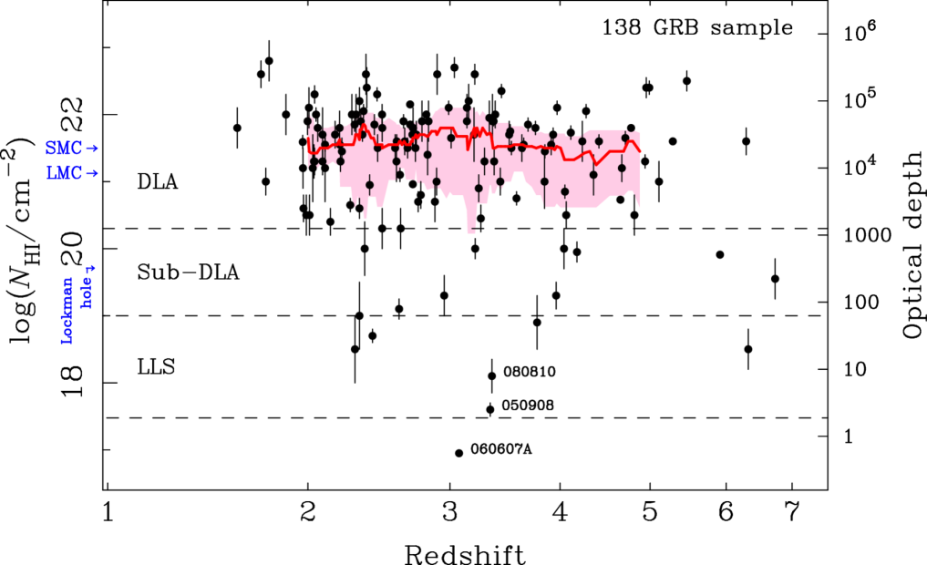
Figure 1: The values of neutral hydrogen column-density in the host plotted against redshift for the sample of GRBs. The corresponding optical depth at the Lyman limit is shown on the right-hand axis. The large majority are DLAs, with a smaller proportion (17/138) being classified as sub-DLAs, Lyman Limit Systems (LLS) and below. All sight-lines apart from the two with the lowest column-densities are essentially opaque ($\tau\gtrsim 10$) to EUV ionizing radiation. The running median (red line) and interquartile range (pink shading) of 20 points shows no evidence for significant variation with redshift. For comparison, on the left axis we also mark the locations of the median log(${N_{{\text{H\,{i}}}}}$/2) values in the directions of LMC and SMC H ii regions from Pellegrini et al. (2012) (halving the measured columns is appropriate since the they include contributions from both the foreground and background of the H ii region), and the lowest column density out of the Milky Way from the position of the Sun, the “Lockman hole" (Lockman et al., 1986).

Table 1: The sample of GRBs. References:- (1) Jensen et al. (2001), (2) Fynbo et al. (2002), (3) Vreeswijk et al. (2006), (4) Hjorth et al. (2003b), (5) Fynbo et al. (2005), (6) Møller et al. (2002), (7) Shin et al. (2006), (8) Vreeswijk et al. (2004), (9) Jakobsson et al. (2004), (10) Fynbo et al. (2009), (11) Berger et al. (2006), (12) Totani et al. (2006), (13) Chen et al. (2007), (14) Chary et al. (2007), (15) Ferrero et al. (2009), (16) This work, (17) Wiseman et al. (2017), (18) Patel et al. (2010), (19) de Ugarte Postigo et al. (2012), (20) Kuin et al. (2009), (21) D’Avanzo et al. (2010), (22) Savaglio et al. (2012), (23) Levesque et al. (2010a), (24) Selsing et al. (2018), (25) Cucchiara et al. (2011b), (26) Zafar et al. in prep., (27) Cucchiara et al. (2015), (28) Jeong et al. (2014), (29)  Chornock et al. (2014), (30) Melandri et al. (2015), (31) Pugliese et al. in prep., (32) Chen et al. (2009), (33) Perley (2011), (34) Schulze et al. (2015), (35) Greiner et al. (2015b), (36) McGuire et al. (2016), (37) Tanvir et al. (2012a), (38) McGuire et al. in prep., (39) Thöne et al. (2011), (40) Friis et al. (2015), (41) Perley et al. (2013), (42) Laskar et al. (2011), (43) Perley et al. (2016b), (44) Myers et al. in prep. (in this case, the derived Spitzer photometry was transformed to stellar mass estimates following Perley et al., 2016b).

GRB	$z$	${{\rm log}\left(\frac{{N_{{\text{H\,{i}}}}}}{{\rm cm}^{-2}}\right)}$	Refs.	$M_{\rm UV,AB}$	Refs.	log(M∗/M⊙)	Refs.
000301C	2.03	$21.20\pm 0.50$	(1)	$-16.0\pm 0.5$	(32)
000926	2.04	$21.30\pm 0.25$	(2)	$-20.40\pm 0.07$	(32)	$9.64$	(41)
011211	2.14	$20.40\pm 0.20$	(3)	$-19.97\pm 0.10$	(32)	$8.0$	(41)
020124	3.20	$21.70\pm 0.40$	(4)	$>-15.72$	(35)	$<9.90$	(42)
021004	2.33	$19.00\pm 0.50$	(5),(6),A.1	$-20.56\pm 0.10$	(5)	$9.45$	(41)
030226	1.99	$20.50\pm 0.30$	(7)
030323	3.37	$21.90\pm 0.07$	(8)	$-18.47\pm 0.1$	(32)	$<9.85$	(42)
030429	2.65	$21.60\pm 0.20$	(9)
050319	3.24	$20.90\pm 0.20$	(10)	$>-20.01$	(33)	$9.69$	(43)
050401	2.90	$22.60\pm 0.30$	(10)	$-19.28\pm 0.31$	(34)	$9.61$	(43)
050505	4.27	$22.05\pm 0.10$	(11)			$<9.67$	(44)
050730	3.97	$22.10\pm 0.10$	(10)	$>-17.21$	(35)	$<9.46$	(43)
050820A	2.61	$21.10\pm 0.10$	(10)	$-18.93\pm 0.06$	(34)	$9.38$	(43)
050904	6.29	$21.60\pm 0.20$	(12)	$-19.21\pm 0.2$	(36)	$<10.07$	(43)
050908	3.34	$17.60\pm 0.10$	(10)	$-18.18\pm 0.27$	(34)	$<9.91$	(42)
050922C	2.20	$21.55\pm 0.10$	(10)	$>-17.95$	(33)	$<9.01$	(43)
060115	3.53	$21.50\pm 0.10$	(10)	$-18.61\pm 0.27$	(34)	$9.43$	(43)
060124	2.30	$18.50\pm 0.50$	(10)
060206	4.05	$20.85\pm 0.10$	(10)	$-18.47\pm 0.1$	(35)	$<9.95$
060210	3.91	$21.55\pm 0.15$	(10)	$-21.85\pm 0.12$	(33)	$10.46$	(43)
060223A	4.41	$21.60\pm 0.10$	(13)	$-18.33\pm 0.15$	(35)	$<10.17$	(42)
060510B	4.94	$21.30\pm 0.10$	(13)	$-20.51\pm 0.17$	(35)	$9.86$	(44)
060522	5.11	$20.60\pm 0.30$	(14),(16)	$>-18.34$	(37)	$<9.31$	(43)
060526	3.21	$20.00\pm 0.15$	(10)	$>-17.36$	(35)	$9.30$	(43)
060605	3.77	$18.90\pm 0.40$	(15)	$-17.94\pm 0.2$	(35)	$<9.97$	(42)
060607A	3.08	$16.95\pm 0.03$	(10)	$>-15.52$	(35)	$<9.45$	(43)
060707	3.43	$21.00\pm 0.20$	(10)	$-20.78\pm 0.06$	(34)	$9.99$	(43)
060714	2.71	$21.80\pm 0.10$	(10)	$-18.88\pm 0.28$	(34)	$9.25$	(43)
060906	3.69	$21.85\pm 0.10$	(10)	$>-20.60$	(35)	$<10.02$	(42)
060926	3.21	$22.60\pm 0.15$	(10)	$-21.59\pm 0.05$	(35)	$10.71$	(42)
060927	5.47	$22.50\pm 0.15$	(10)	$>-18.01$	(37)	$<9.63$	(43)
061110B	3.44	$22.35\pm 0.10$	(10)	$-19.82\pm 0.29$	(35)	$<9.47$	(43)
070110	2.35	$21.70\pm 0.10$	(10)	$-19.81\pm 0.11$	(34)	$<9.16$	(43)
070411	2.95	$19.30\pm 0.30$	(10)
070506	2.31	$22.00\pm 0.30$	(10)	$-18.80\pm 0.21$	(34)
070611	2.04	$21.30\pm 0.20$	(10)	$>-17.52$	(34)
070721B	3.63	$21.50\pm 0.20$	(10)	$-18.39\pm 0.44$	(35)	$<9.42$	(43)
070802	2.45	$21.50\pm 0.20$	(10)	$-19.85\pm 0.2$	(34)	$9.69$	(41)
070810A	2.17	$21.70\pm 0.20$	(16)
071031	2.69	$22.15\pm 0.05$	(10)
080129	4.35	$21.10\pm 0.30$	(16)			$<11.47$	(44)
080210	2.64	$21.90\pm 0.10$	(10)	$>-19.32$	(33)	$<9.50$	(43)
080310	2.43	$18.70\pm 0.10$	(10)	$>-18.45$	(33)	$9.78$	(43)
080413A	2.43	$21.85\pm 0.15$	(10)			$<9.64$	(43)
080603B	2.69	$21.85\pm 0.05$	(10)			$9.15$	(43)
080607	3.04	$22.70\pm 0.15$	(10)	$-19.4\pm 0.5$	(35)	$10.45$	(43)
080721	2.59	$21.60\pm 0.10$	(10)			$<9.63$	(43)
080804	2.20	$21.30\pm 0.15$	(10)			$9.28$	(43)
080810	3.36	$18.10\pm 0.25$	(17),A.6	$-22.43\pm 0.5$	(35)	$10.29$	(44)
080905B	2.37	$22.60\pm 0.30$	(16)
080913	6.73	$19.55\pm 0.30$	(18),A.8	$>-17.28$	(38)
081008	1.97	$21.59\pm 0.10$	(19)			$9.18$	(43)
081029	3.85	$21.45\pm 0.10$	(16)	$>-19.87$	(35)	$<9.39$	(43)
081118	2.58	$21.50\pm 0.20$	(16)			$9.18$	(43)
081203A	2.05	$22.00\pm 0.10$	(20)

Table 2: continued

GRB	$z$	${{\rm log}\left(\frac{{N_{{\text{H\,{i}}}}}}{{\rm cm}^{-2}}\right)}$	Refs.	$M_{\rm UV,AB}$	Refs.	log(M∗/M⊙)	Refs.
081222	2.77	$20.80\pm 0.20$	(16)			$9.61$	(43)
090205	4.65	$20.73\pm 0.05$	(21)	$-21.26\pm 0.13$	(35)	$<10.7$	(21)
090313	3.38	$21.30\pm 0.20$	(16)	$>-21.19$	(35)	$<10.35$	(44)
090323	3.58	$20.75\pm 0.10$	(22),A.13	$-21.60\pm 0.18$	(35)	$10.58$	(44)
090426	2.61	$19.10\pm 0.15$	(23),A.14	$-20.43\pm 0.08$	(39)
090516A	4.11	$21.73\pm 0.10$	(19)	$-20.99\pm 0.4$	(35)	$10.63$	(44)
090519	3.85	$21.00\pm 0.40$	(16)	$>19.09$	(35)	$<10.35$	(43)
090529	2.62	$20.30\pm 0.30$	(16)
090715B	3.01	$21.65\pm 0.15$	(16)			$10.20$	(44)
090726	2.71	$21.80\pm 0.30$	(16)
090809	2.74	$21.70\pm 0.20$	(24)
090812	2.45	$22.30\pm 0.10$	(19)			$<9.35$	(43)
090926A	2.11	$21.55\pm 0.10$	(24)
091029	2.75	$20.70\pm 0.15$	(16)			$<9.81$	(43)
100219A	4.67	$21.20\pm 0.20$	(24)	$-19.74\pm 0.5$	(35)	$<10.11$	(44)
100302A	4.81	$20.50\pm 0.30$	(16)
100316A	3.16	$22.20\pm 0.25$	(16)
100425A	1.76	$21.00\pm 0.20$	(24)
100513A	4.77	$21.80\pm 0.05$	(16)	$-19.88\pm 0.29$	(35)	$<10.14$	(44)
100728B	2.11	$21.20\pm 0.50$	(24)			$<9.25$	(43)
110128A	2.34	$21.90\pm 0.15$	(24)
110205A	2.21	$21.45\pm 0.20$	(25)			$9.72$	(43)
110731A	2.83	$21.90\pm 0.30$	(16)
110818A	3.36	$21.90\pm 0.40$	(24)	$-21.68\pm 0.05$	(35)
111008A	4.99	$22.40\pm 0.10$	(24)	$>-20.80$	(35)
111107A	2.89	$21.00\pm 0.20$	(24)
120119A	1.73	$22.60\pm 0.20$	(24)			$9.91$	(43)
120327A	2.81	$22.00\pm 0.05$	(24)
120404A	2.88	$20.70\pm 0.30$	(24)
120712A	4.17	$19.95\pm 0.15$	(24)			$<9.82$	(44)
120716A	2.49	$22.00\pm 0.15$	(24)
120811C	2.67	$21.50\pm 0.15$	(16)
120815A	2.36	$22.05\pm 0.10$	(24)
120909A	3.93	$21.70\pm 0.10$	(24)	$-21.16\pm 0.12$	(35)
121024A	2.30	$21.85\pm 0.10$	(24)	$-21.47\pm 0.10$	(40)	$9.9$	(40)
121027A	1.77	$22.80\pm 0.30$	(24),A.25
121128A	2.20	$21.80\pm 0.25$	(16)
121201A	3.39	$22.00\pm 0.20$	(24)	$-20.84\pm 0.21$	(35)
121229A	2.71	$21.70\pm 0.20$	(24)
130408A	3.76	$21.80\pm 0.10$	(24)	$>-21.13$	(35)
130427B	2.78	$21.90\pm 0.30$	(24)
130505A	2.27	$20.65\pm 0.10$	(27)
130518A	2.49	$21.80\pm 0.20$	(16)
130606A	5.91	$19.91\pm 0.02$	(24)	$-20.33\pm 0.15$	(36)
130610A	2.09	$21.30\pm 0.20$	(16)
130612A	2.01	$22.10\pm 0.30$	(24)
131011A	1.87	$22.00\pm 0.30$	(24)
131108A	2.40	$20.95\pm 0.15$	(16)
131117A	4.04	$20.00\pm 0.30$	(24)
140206A	2.73	$21.50\pm 0.20$	(16)
140226A	1.97	$20.60\pm 0.20$	(27)
140304A	5.28	$21.60$	(28)
140311A	4.95	$22.40\pm 0.15$	(24)			$<10.10$	(44)
140419A	3.96	$19.30\pm 0.20$	(27)
140423A	3.26	$20.45\pm 0.20$	(27)
140430A	1.60	$21.80\pm 0.30$	(24)
140515A	6.32	$18.50\pm 0.30$	(29),(30),A.31	$-18.31\pm 0.35$	(36)
140518A	4.71	$21.65\pm 0.10$	(27)
140614A	4.23	$21.60\pm 0.30$	(24)
140629A	2.28	$22.00\pm 0.30$	(16)
140703A	3.14	$21.90\pm 0.10$	(16)
140808A	3.29	$21.30\pm 0.20$	(16)
141028A	2.33	$20.60\pm 0.15$	(24)
141109A	2.99	$22.10\pm 0.10$	(24)

Table 3: continued

GRB	$z$	${{\rm log}\left(\frac{{N_{{\text{H\,{i}}}}}}{{\rm cm}^{-2}}\right)}$	Refs.	$M_{\rm UV,AB}$	Refs.	log(M∗/M⊙)	Refs.
150206A	2.09	$21.70\pm 0.40$	(24)
150403A	2.06	$21.80\pm 0.20$	(24)
150413A	3.14	$22.10\pm 0.20$	(16)
150915A	1.97	$21.20\pm 0.30$	(24)
151021A	2.33	$22.20\pm 0.20$	(24)
151027B	4.06	$20.50\pm 0.20$	(24)
151215A	2.59	$21.30\pm 0.30$	(16)
160203A	3.52	$21.75\pm 0.10$	(24),(31)
160227A	2.38	$22.40\pm 0.30$	(16)
160629A	3.33	$21.95\pm 0.25$	(16)
161014A	2.82	$21.40\pm 0.30$	(24)
161017A	2.01	$20.50\pm 0.30$	(16)	$>-20.11$	(16)
161023A	2.71	$20.96\pm 0.05$	(24)
170202A	3.65	$21.55\pm 0.10$	(24)
170405A	3.51	$21.70\pm 0.20$	(16)
170531B	2.37	$20.00\pm 0.40$	(16)
180115A	2.49	$20.30\pm 0.30$	(16)
180325A	2.04	$22.30\pm 0.14$	(26)
180329B	2.00	$21.90\pm 0.20$	(16)

3 Implications for the ionizing escape fraction

Following Chen et al. (2007), we note that the optical depth for radiation at the Lyman limit (912 Å) along a given sight line due to absorption by neutral hydrogen is given by $\tau=\sigma_{\rm LL}{N_{{\text{H\,{i}}}}}$, where $\sigma_{\rm LL}=6.28\times 10^{-18}$ cm² is the photoionization cross-section of hydrogen. Hence the average escape fraction for $n$ sight lines is given by

$$\langle{f_{\rm esc}}\rangle=\frac{1}{n}\sum\limits_{i=1}^{n}{{\rm exp}(-\tau_{i})}.$$ (1)

Considering our whole sample, we find a mean value of only $\langle f_{\rm esc}\rangle=0.005$, well below that thought to be required in the EoR.

In Figure 2 we plot the cumulative distribution of H i column-density measures for the whole sample. The median value of column-density is ${\rm log}({N_{{\text{H\,{i}}}}}/{\rm cm}^{-2})=21.59$, consistent with previous studies (e.g. the equivalent figure is 21.5 for the sample of Fynbo et al., 2009) and also similar to the median values of ${\rm log}({N_{{\text{H\,{i}}}}})$ towards H ii regions in the Magellanic Clouds (Pellegrini et al., 2012, see Figure 1). We find that up to the median point the sample is well described by a simple power law distribution $P(<x)\propto x^{0.4}$, where $x$ is the value of ${N_{{\text{H\,{i}}}}}$, shown as an orange dashed line in the figure. While this model is not motivated by any particular physical considerations, it does provide a smooth representation of the data, and using it we obtain an average escape fraction $\langle f_{\rm esc}\rangle=0.004$, in good agreement with the value found above.

Most of the rest of this paper is concerned with the robustness of this result, and the statistical and potential systematic uncertainties that may affect it.

3.1 Low column-density sight-lines

Only two sight-lines have ${\rm log}({N_{{\text{H\,{i}}}}}/{\rm cm}^{-2})<18$ (corresponding to $f_{\rm esc}>0.002$), and as it happens both of these low column-density systems were already included in the Chen et al. (2007) and Fynbo et al. (2009) analyses. Since the numerical result for $\langle{f_{\rm esc}}\rangle$ depends entirely on these two sight-lines, we review here what is known of their properties and in particular consider whether there could be attenuation of EUV radiation by dust as well as H i absorption. We also address the effect of direct recombinations to the ground-state producing ionizing photons.

3.1.1 GRB 050908

GRB 050908, at $z=3.34$, had a moderately bright optical afterglow, being $R\approx 19$ at 15 min post-burst (Torii, 2005). Spectroscopy was obtained with Gemini/GMOS, from which Chen et al. (2007) reported a column-density of ${\rm log}({N_{{\text{H\,{i}}}}}/{\rm cm}^{-2})=19.1$. The lower value of ${\rm log}({N_{{\text{H\,{i}}}}}/{\rm cm}^{-2})=17.6$, corresponding to $f_{\rm esc}=0.08$, used here, was that derived from a VLT/FORS1 spectrum (Fynbo et al., 2009), and it is preferred since it is based on direct evidence of non-zero afterglow continuum emission below the Lyman limit.

There is no indication of excess absorption in the Swift X-ray observations (Evans et al., 2009), which is also consistent with a low column density and low extinction sight-line.

3.1.2 GRB 060607A

GRB 060607A, at $z=3.08$, had a very bright and well-studied early optical afterglow, which reached $r=14.3$ at 3 min post-burst (Nysewander et al., 2009). This sight-line has the lowest column-density of our sample at ${\rm log}({N_{{\text{H\,{i}}}}}/{\rm cm}^{-2})=16.95$, from a VLT/UVES spectrum (Fynbo et al., 2009), corresponding $f_{\rm esc}=0.57$. The spectrum also showed evidence for emission below the Lyman limit, although only for a small stretch of wavelength before it was cut-off by an intervening absorber, but this is consistent with a very low opacity.

The light curve and spectral energy distribution were studied in detail by Nysewander et al. (2009), who modelled their Bgri optical data together with $H$-band photometry from Molinari et al. (2007). They concluded that a rest-frame dust extinction of zero was ruled out at the $2.6\sigma$ level. The shape of the extinction law is only weakly constrained by these data, so extrapolating to the Lyman limit introduces a large systematic uncertainty, but with reasonable dust laws their favoured extinction would correspond to a value of $A_{912}\gtrsim 1$. If this inference is correct, then it would suggest the actual escape fraction at the Lyman limit for GRB 060607A could be significantly diminished by dust extinction, by a factor $\sim 2.5$ or more.

We note that there is also marginal evidence of X-ray absorption in the source-frame at a level of $N_{\rm H,X}\approx(3.1\pm 1.9)\times 10^{21}$ cm^-2 (Evans et al., 2009) over the Milky Way foreground (Willingale et al., 2013). This would be broadly consistent with a SMC dust-to-gas ratio (Bouchet et al., 1985) providing the hydrogen associated with this gas had largely been ionized (so it was not seen in the optical spectrum) but the dust had mostly not been destroyed. On the other hand, Prochaska et al. (2008) argue that the absence of N v absorption argues for both low density and low metallicity surrounding the burst location.

3.1.3 Direct recombinations to the ground-state

Gas that has been ionized by massive star radiation within a host galaxy will generally recombine quickly. A fraction of recombining H ions will go directly to the ground-state, and so emit a photon just above the Lyman limit energy (some higher energy photons will also be emitted by recombining He ions). In low column-density systems a fraction of these will escape the host without further absorption, and therefore re-boost the escaping ionizing flux, albeit with radiation that will soon be redshifted to energies below 1 Ryd. In other words, simply translating H i column-density into line-of-sight opacity is likely to lead to a small underestimate of the escape fraction in low column-density systems. The net effect of this re-boost depends on various factors, but could provide an increase of up to 10–20% in the effective escape fraction (Faucher-Giguère et al., 2009), thus at least partially offsetting any dust extinction.

For the remainder of Section 3 we will continue to consider only the opacity due to H i absorption, but will return to the potential systematic effects of dust in Section 4.1.1.

3.2 Statistical uncertainty

Even with our considerably larger sample of sight-lines, the fact that only two have any appreciable escape fraction means that to some extent we are still dealing with rather small number statistics. We also lack a robust theoretical model which could be fit to the data, and so must explore the statistical uncertainties non-parametrically.

Again we first follow Chen et al. (2007) by performing a bootstrap exercise, employing $10^{6}$ random resamples of the data with replacement. From this we estimate a 98% confidence upper limit of $\langle{f_{\rm esc}}\rangle<0.015$; the result is the same whether or not we allow the resampled ${N_{{\text{H\,{i}}}}}$ values to have additional scatter based on the error bars for each point.

In an alternative approach, we simulated several large populations of sight-lines with higher values of average escape fraction than found in our data (by replicating the GRB 050908/060607A values), and drew $10^{5}$ random 138-member samples from each of these. For the case of the population with $\langle{f_{\rm esc}}\rangle_{\rm pop}=0.02$ we found 98% of random samples produced $\langle{f_{\rm esc}}\rangle_{\rm samp}>0.005$. Thus, these two methods agree on an upper limit for $\langle{f_{\rm esc}}\rangle$ of $0.015$–$0.02$. A similar analysis gives a 98% lower limit of $\langle{f_{\rm esc}}\rangle>10^{-3}$.

These are significantly tighter constraints than found by the previous studies of Chen et al. (2007) and Fynbo et al. (2009) of $\langle{f_{\rm esc}}\rangle<0.075$ at 95%, due to our larger sample size and the fact that no further very low column-density sight-lines have been identified in any of the additional GRBs. We note that our result is also consistent with the $\langle{f_{\rm esc}}\rangle=0.020\pm 0.017$ obtained by constraining the flux below the Lyman-limit in a stacked spectrum of eleven GRB afterglows with $\bar{z}=3.66$ by Christensen et al. (2011).

3.3 Comparison to model predictions

It is worth noting that our ${N_{{\text{H\,{i}}}}}$ distribution is inconsistent with the predictions of Cen & Kimm (2014) who used high-resolution cosmological radiation-hydro simulations of galaxies within the EoR ($z\sim 7$) to explore column-densities along GRB sight-lines. They found a bimodal distribution with a peak at high column-density (${\rm log}({N_{{\text{H\,{i}}}}}/{\rm cm}^{-2})\sim 21$–22), similar to the observed distribution, but then another substantial peak with column-densities ${\rm log}({N_{{\text{H\,{i}}}}}/{\rm cm}^{-2})<18$ which is not seen in practice. Part of the explanation could be that Cen & Kimm (2014) assumed that the GRB rate traces the SNII rate and found a large fraction of their low column-density GRBs occurred in super-solar metallicity environments, whereas in reality GRB progenitors seem to be younger at explosion (e.g. Larsson et al., 2007) and crucially, unlike SNII, are rarely found in high metallicity galaxies (e.g. Perley et al., 2015). On the other hand, their simulations do not account for the effect of GRBs in ionizing gas local to the burst (see Section 4.1.2), and it seems when a high column-density is found in their models it is often due to such local gas, whereas the low column-density cases occur for progenitors that have escaped their birth clouds. This suggests their simulations do not capture the distributed nature of neutral hydrogen in these star-forming galaxies, at least as it is found in $z\sim 2$–5 GRB hosts.

Our results do correspond much more closely with the earlier simulations of Pontzen et al. (2010), who similarly investigated sight-lines to young star forming regions in model galaxies, but in this case did specifically consider the $z\sim 2$–5 range. They found a median ${\rm log}({N_{{\text{H\,{i}}}}}/{\rm cm}^{-2})$ of 21.5 and calculated an escape fraction of $\langle{f_{\rm esc}}\rangle\approx 0.01$, both close to our findings. Indeed, their default prescription assumes that GRBs trace star formation up to an age of 50 Myr, whereas restricting to a perhaps more realistic 10 Myr age reduces $\langle{f_{\rm esc}}\rangle$ to 0.007. These simulations included the effect of local ionizing sources on the gas proximate to the burst, but again not the potential additional effect of ionization due to the GRB itself. We return to these issues in Section 4.

3.4 Evolution with redshift

As shown by the red line in Figure 1, there is no evidence for significant variation in the median value of ${\rm log}({N_{{\text{H\,{i}}}}})$ between redshifts $z\sim 2$ to $z\sim 5$. To investigate this further, in Figure 2 we plot cumulative ${N_{{\text{H\,{i}}}}}$ distributions for three subsets of the whole sample cut in redshift. It is apparent that there is little difference between the low ($z<3$) and intermediate redshift ($3<z<5$) sub-samples – the median values are the same, and a two-sample Kolmogorov-Smirnov (KS) test finds them to be consistent with the null hypothesis that they are drawn from the same parent distribution (p-value of 0.88). The intermediate redshift sub-sample does have a somewhat longer tail to low column-density than the low redshift sub-sample, and we note that low column-density systems are arguably rather more likely to go unrecognised at lower redshifts (discussed further in Section 4.2.2). However, another potential selection effect is that the proportion of dusty sight-lines appears to decline with increasing redshift above $z\sim 3$ (Kann et al., 2010; Perley et al., 2016a, b), and if dusty bursts are systematically lost from the low redshift sub-sample, due to the difficulty of locating and obtaining spectra for the afterglows, then it could mask a more significant evolutionary trend. The issue of biases due to dust is one we return to in subsequent sections.

There is a suggestion of a more significant decline in the typical values of ${\rm log}({N_{{\text{H\,{i}}}}})$ at $z\gtrsim 6$ (as also pointed out by Chornock et al., 2014; Melandri et al., 2015), which influences the final $z>5$ bin (red line). However, the conclusion is still limited by small number statistics, and a KS test again finds this $z>5$ sub-sample to be consistent with being drawn from the same distribution as the lower redshift ($z<5$) sub-sample (p-value of 0.31).

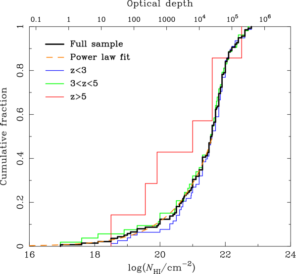
Figure 2: Cumulative distribution of H i for the whole sample and split into subsets by redshift, as indicated. The corresponding optical depth at Ly$\alpha$ is shown on the top axis. A power-law fit to the lower column-density half of the sample is shown by the orange dashed line (see text).

3.5 Dependence on host properties

In Figure 3 we plot ${\rm log}({N_{{\text{H\,{i}}}}})$ versus host UV absolute magnitude, $M_{\rm UV}$, which is a gauge of the current (unobscured) star formation rate, for those bursts in our sample where good constraints on host luminosity are available in the literature (37 measurements and 18 upper limits, detailed in Table 1). The restricted number of cases for which deep host searches have been conducted, and the fact that many are upper limits, means we cannot draw firm conclusions, but there is little indication of a dependence of the average H i column-density on the current star formation rate. Note, we have converted these values to a common cosmology (a flat Friedmann model with $\Omega_{\rm M}=0.3$, $H_{0}=70$  km s^-1), but not otherwise attempted to correct for differences in the procedures used by different authors (approaches to k-corrections, for example), or small deviations from the reference 1600 Å wavelength generally adopted. These distinctions should not be at a level that would affect the conclusion.

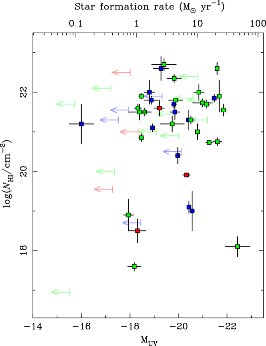
Figure 3: The values of neutral hydrogen column-density plotted against host rest-frame UV absolute AB magnitude and corresponding star formation rate (top axis, following the calibration for a $Z=Z_{\odot}/3$, constant star-formation rate and age $>300$ Myr population from Madau & Dickinson, 2014), for 37 detections and 19 upper limits collected from various sources (Table 1). Colour coding is as with the lines in Figure 2 and upper limits are $2\sigma$.

Similarly, in Figure 4 we plot ${\rm log}({N_{{\text{H\,{i}}}}})$  against host stellar mass, ${\rm M_{*}}$, for those galaxies in our sample for which estimates (or limits) are available in the literature (Table 1). The bulk are based on Spitzer infrared photometry, particularly from Perley et al. (2013), Perley et al. (2016b), Laskar et al. (2011) and Myers et al. in prep. Here we are restricted to 28 galaxies with ${\rm M_{*}}$ estimates and 31 galaxies with upper limits. Again there is little indication of any trend, contrary to suggestions that $f_{\rm esc}$ may correlate strongly with galaxy size (e.g Anderson et al., 2017).

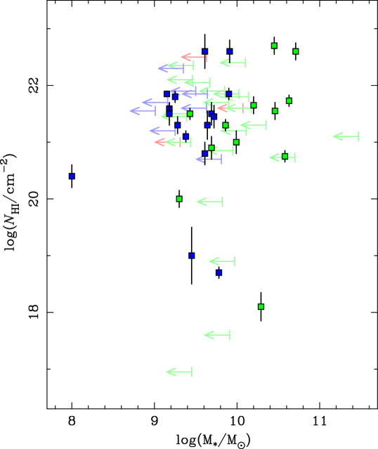
Figure 4: The values of neutral hydrogen column-density plotted against host stellar mass estimates from a range of sources (Table 1) for 60 hosts, 32 of which are upper limits (shown at 2$\sigma$). Colour coding is as with the lines in Figure 2. The approximate stellar masses of the Milky Way and Magellanic Clouds are indicated on the top axis for comparison.

One trend that is conspicuous in Figure 3, and in particular Figure 4, is that the UV brighter and more massive hosts are predominantly in the $3<z<5$ bin. It is true that small and faint hosts are harder to detect at higher redshifts, and that may explain some part of this trend. However, another factor seems to be that higher mass (${\rm M}_{*}\gtrsim 10^{10}$ M_⊙) hosts at $z<3$ are more often associated with heavily extinguished bursts, and hence more likely to be highly dusty, than at higher redshifts (Perley et al., 2016b); these are presumably systematically under-represented in our compilation.

4 Potential systematic uncertainties

A number of systematic uncertainties may affect our analysis, potentially biasing the conclusions. These include observational selection effects: in order to be included in the sample afterglows must be localised and spectra obtained which cover the Ly$\alpha$ region with reasonable signal-to-noise.

Other concerns relate to the still-uncertain nature of the GRB progenitor itself, both in terms of the assumption that their sight-lines are representative of dominant EUV-producing stars, and specifically whether there could be special circumstances required to produce GRBs that necessitate an atypical environment. It is also pertinent to ask whether the results can be extrapolated to the EoR.

In this section we begin by investigating systematic effects which may influence our calculation of $\langle{f_{\rm esc}}\rangle$ in terms of its application to the GRB progenitors. The majority ($\sim 70$%; Gehrels & Razzaque, 2013) of Swift-discovered GRBs do not have redshifts, which, it may be thought, could lead to large biases. With a more uniformly selected sample, some of these effects might be quantified via simulated data-sets, but that approach would be of limited utility here. However, by considering the nature of these selection effects, and surveying the available data, we shall show that these biases can be understood well enough to confirm that they are unlikely to affect the main conclusions.

We then consider more carefully how representative the GRB progenitors are of the EUV-producing massive stars, and the potential systematic uncertainties that may introduce. Finally we discuss in more detail the application of our results to the EoR.

4.1 Systematic over-estimation of $\langle{f_{\rm esc}}\rangle$

Two factors are very likely to produce an over-estimate of the escape fraction, as discussed here.

4.1.1 Dust extinction biases

GRB afterglow surveys are biased against high column-density sight-lines since they tend to be dustier and hence harder to locate and obtain redshifts for in the optical band (Fynbo et al., 2009; Greiner et al., 2011; Watson & Jakobsson, 2012). Dusty systems at higher redshift would be particularly susceptible to being lost since even near-IR observations will be looking in the source-frame optical or near-UV. However we expect dusty systems to be rarer at $z\gtrsim 4$ (Perley et al., 2016b) and particularly by $z\sim 6$ (cf. Zafar et al., 2011; Schaerer et al., 2015). Recently Bolmer et al. (2018) have shown that the decline of obscuration in GRB afterglows with increased redshift is likely primarily due to their hosts being less dusty rather than an observational selection effect.

Over all redshifts, Perley et al. (2016a) estimate that approximately 20% of GRBs detected by Swift are heavily dust obscured, and often reside in globally dusty, massive galaxies (Rossi et al., 2012; Perley et al., 2013); this sub-population is significantly biased against in afterglow samples. A similar proportion show signs of more moderate dust obscuration (see also Covino et al., 2013). Thus this effect, while important for understanding the overall GRB host population, would likely only necessitate a comparatively minor correction to the escape fraction estimate (i.e. a $\sim 20$–40% reduction, assuming that all very dusty sight-lines are opaque to EUV), and the correction is likely to be greatest at $z<3$, as discussed in Section 3.4.

Even in some cases where afterglows have been detected and redshifts measured, there may be significant attenuation in the UV by dust. However, from the point of view of escape fraction, this is only relevant for the two sight-lines with non-negligible $f_{\rm esc}$, and as already discussed in Section 3.1 may lead to corrections (downward) of a factor $\sim 2$ or more for our sample.

4.1.2 Effects of GRB prompt emission and early afterglow on local gas and dust

The GRB prompt flash and early afterglow produces an intense radiation field that is expected to quickly destroy dust (Waxman & Draine, 2000; Morgan et al., 2014) and ionize gas to distances of up to several tens of pc when the ambient medium has a low to moderate density, $n\lesssim 10$ cm^-3 (Perna & Lazzati, 2002; Vreeswijk et al., 2007; Krongold & Prochaska, 2013). Therefore the opacity measured to the afterglow could in principle be less than the opacity that would have been seen to the progenitor star system. Various lines of evidence suggest the existence of an ionized gas component, likely reasonably local to the GRB. In particular, it has been argued that high column-densities measured in X-ray absorption, which in some afterglows significantly exceed the optical measures, are at least partially due to denser gas close to the progenitor in which the hydrogen has been ionized (Watson et al., 2007; Schady et al., 2011). Furthermore, the observed correlation of X-ray absorption with local galaxy surface brightness (in optically bright GRBs) may support a local origin for a significant proportion of the absorbing gas (Lyman et al., 2017). Highly ionized species have also been seen in some afterglow spectra, which are likely to be of circumburst origin (Fox et al., 2008; De Cia et al., 2011, Heintz et al. submitted.).

On the other hand, significant ionization may have been brought about by the stellar radiation field prior to the burst (Watson et al., 2013; Krongold & Prochaska, 2013), rendering the ionizing effect of the GRB largely irrelevent. This is supported by models of feedback from star formation in massive molecular clouds which show that hot ionized bubbles can grow to tens or hundreds of pc in a few Myr, although in some circumstances, in particular if star formation is relatively inefficient, the outflow can stall and the cloud recollapse, leading to further star formation episodes (e.g. Rahner et al., 2017).

In principle, deep time-resolved spectroscopy may allow the GRB-driven ionization of H i to be observed directly (Perna & Lazzati, 2002), although in practice, sufficiently good data-sets have rarely been acquired. Only in one case, namely GRB 090426, has time-variability of Ly$\alpha$ been seen, between spectra obtained at 1.1 hr and 12 hr post-burst, suggesting the influence of the GRB. Here photoionization modelling placed the absorbing gas at $\sim 80$ pc (Thöne et al., 2011). As discussed in Appendix A.14, there is uncertainty regarding this particular burst as to whether it is of the long or short duration class, but nonetheless it confirms the local ionizing effect of GRB emission can occur even at quite large distances.

In one other case, GRB 080310, Vreeswijk et al. (2013) found their time-dependent photoionization model to be improved with the addition of a cloud at $\sim 10$–50 pc from the burst, which became fully ionized by the early afterglow emission. The required column-density of this cloud, of ${\rm log}({N_{{\text{H\,{i}}}}}/{\rm cm}^{-2})\sim 19$–20, was greater than the ${\rm log}({N_{{\text{H\,{i}}}}}/{\rm cm}^{-2})=18.7$ inferred for the observed neutral absorber.

In conclusion, it is likely that some fraction of GRBs exhibit a reduced H i column-density due to the ionizing effect of the burst itself. If windows to the IGM often occur when superbubbles puncture low-density channels out of galactic neutral gas (e.g. Dove et al., 2000; Roy et al., 2015), then this may be largely irrelevant as far as high escape fraction sight-lines are concerned. On the other hand, regarding our sample, if GRB 060607A was dust extinguished (Section 3.1.2) then it would be surprising if the dust was not associated with some neutral gas which was ionized by the burst.

4.2 Systematic under-estimation of $\langle{f_{\rm esc}}\rangle$

A reasonable question is whether some very low ${N_{{\text{H\,{i}}}}}$ systems may not have been recognised in GRB afterglow observations. Omitting from our sample, or over-estimating the column-density, of even a fairly small number of such bursts could lead to significant under-estimation of $\langle{f_{\rm esc}}\rangle$. There are several circumstances in which this could plausibly arise that are discussed below. The nature of such biases depends on the quality of the afterglow spectroscopy, and so we split our discussion into three broad categories: good S/N spectra (Sections 4.2.2 and 4.2.3), poor S/N spectra that were still sufficient to provide a redshift (Section 4.2.5), and instances where no redshift was obtained due to the faintness of the optical afterglow (Section 4.2.6). These divisions are somewhat qualitative, but this is appropriate given that we do not have access to many individual spectra, and also noting that continuum S/N can vary significantly within a spectrum.

However, first we consider what can be said about the potential level of such selection effects, by reference to a nearly redshift-complete GRB sample.

4.2.1 Lessons from the SHOALS sample

Only a fraction of X-ray localised GRBs have optical/nIR afterglow identifications, and only a fraction of those have redshifts from afterglow spectra. Thus, if the chances of a redshift being obtained depend on the H i column-density then it could bias our results. On the other hand, many GRBs receive little ground-based follow-up for other reasons, for example, because of poor weather at major observatories, because they are badly placed for observation due to proximity to the Sun, Moon or Galactic plane, or simply because of the limited availability of large telescopes to make the necessary rapid target-of-opportunity observations.

Since our sample is not selected or observed in a uniform way, and many values are taken from the literature, it is hard to assess the maximum scale of these effects directly. However, we can get a handle on them by considering the well-defined Swift Gamma-Ray Burst Host Galaxy Legacy Survey (SHOALS) sample (Perley et al., 2016a), which consists of 119 long-duration GRBs discovered by Swift up until October 2012, and excludes bursts that were poorly placed for ground observation (whether or not they have redshifts). SHOALS imposes a threshold on the prompt $\gamma$-ray fluence of $S_{15-150\,\rm keV}>10^{-6}$ erg cm^-2, which does mean it excludes some intrinsically very weak events, but prompt emission is thought to arise from internal processes within the GRB jet and so not to be dependent on the nature of the ambient environment. Furthermore, despite many searches, there is little indication that prompt $\gamma$-ray behaviour depends on other properties of the host, such as metallicity (e.g. Levesque et al., 2010b; Japelj et al., 2016). SHOALS also requires that bursts have identified X-ray counterparts, but since all long-bursts are detectable in X-rays if observed sufficiently early by Swift, the selection criterion employed was simply that a rapid autonomous slew was performed. This is consistent with theoretical expectations that the X-ray afterglow flux should be independent of ambient density, $n$, unless it is very low ($n<10^{-3}$ cm^-3, e.g. Hascoët et al., 2011).

The SHOALS sample has a high degree of redshift completeness thanks in large part to major efforts to obtain redshifts from host galaxy observations (identified within X-ray or optical afterglow error boxes) where they had not already been obtained from afterglow spectroscopy. Specifically, 92% have spectroscopic or (in a few cases) good photometric redshifts, and all but one have some photometric constraint on the redshift.

Here we restrict our attention to the 80 bursts for which the redshift is $z>1.6$ or for which the constraints allow the possibility of the burst being in that range. Of these we can immediately say that 52 were very likely high column-density sight-lines, either because ${N_{{\text{H\,{i}}}}}$ was measured directly (39) or because they were found to have faint afterglows with indications of high levels of extinction (14) according to Perley et al. (2016a, see also Section 4.1.1). One, namely GRB 060607A, is the same low-column system included in our sample.

Of the remainder, 19 appear to have had at least moderately bright optical afterglows, but either spectroscopy was obtained which did not cover the wavelength of Ly$\alpha$ (8) and the redshifts rely on metal lines (although in no case were these lines reported as being unusually weak) or simply no spectroscopy was attempted to our knowledge (11). A further four had little afterglow follow-up of any kind reported; these were GRB 050128, early in the Swift mission, GRB 050726, for which real-time alerts were not sent to the ground, GRBs 050922B which occurred on the same day as several other high-priority bursts, and GRB 070328. We find no reason to think any of these bursts lacked Ly$\alpha$ measurements due to observational selection effects, since they all seem to be cases where only limited follow-up was attempted.

This leaves only three sources, which merit more thorough scrutiny. One of these, GRB 071025, was observed with Keck/HIRES, but the spectrum was low-S/N with flux only being detected at $\lambda>7500$ Å. Fynbo et al. (2009) argued that this may be due to a Ly$\alpha$ break at $z\approx 5.2$ (the low S/N precluding measurement of the line strength), or alternatively that it could indicate a highly dust reddened afterglow at lower redshift. A photometric redshift constraint from multi-band afterglow imaging supports a high redshift ($z\sim 5$) interpretation, whilst also favouring fairly substantial dust extinction (Perley et al., 2010). Thus it seems this is an intrinsically bright event but, again, most likely with a high column-density sight-line.

GRB 100305A was the target of several deep imaging observations within the first hour post-burst, but the only candidate afterglow (Gemini/GMOS observations in $riz$; Cucchiara, 2010) was subsequently found to be outside the revised X-ray error circle and to be present as a steady source in later imaging (Perley et al., 2016a). We have analysed previously unpublished early UKIRT data, and also find no afterglow down to a 2$\sigma$ limit of $K_{\rm AB}=20.7$ at 40 min after the trigger. In fact the Swift/XRT spectrum (see http://www.swift.ac.uk/xrt_spectra/00414905/; Evans et al., 2009) does show significant X-ray absorption above the Galactic value, suggesting a high column sightline, possibly combined with moderately high redshift making the optical/nIR afterglow faint.

Finally we have GRB 070223 is known to be at redshift $z=1.63$ from the host galaxy (Perley et al., 2016a). Here the afterglow was faint in both the optical and near-infrared, despite early follow-up, meaning that no spectroscopy was attempted. The host galaxy was detected in Spitzer 3.6 $\mu$m imaging, but the implied stellar mass is a relatively modest ${\rm{log(M_{*}/M_{\odot})}\approx 9.5}$ (Perley et al., 2016b). We have reanalysed the early imaging obtained at the Liverpool Telescope and the WHT at $\approx 3$ hr post-burst (details are given in Appendix A.3), finding AB magnitudes of $r=23.8\pm 0.3$ and $K=22.0\pm 0.3$ for a faint source at the X-ray afterglow position. However, we have also analysed the SDSS and PanSTARRS imaging of the same region, and in both cases find a persistent source, presumably the host, at the same location, with a magnitude $r=23.5\pm 0.3$. Thus it seems clear that the optical source seen by the LT (and also the MDM 1.3m; Mirabal et al., 2007) was actually host dominated, and hence the optical afterglow must have been substantially fainter. By contrast, the $K$-band source faded by 0.7 mag by the following week, confirming an afterglow detection in the near-IR (Rol et al., 2007). Thus it seems likely that, despite not being in a massive dusty host, this event too was heavily extinguished, which is consistent with the high column-density inferred from the X-ray spectrum of ${\rm log}(N_{\text{H\,{i}}\rm,X}/{\rm cm}^{-2})\approx{22.6}$ (see http://www.swift.ac.uk/xrt_spectra/00261664/; Evans et al., 2009).

In summary, from our analysis of the SHOALS sample, of 80 bursts that may be at $z>1.6$, 55 have evidence of high-${N_{{\text{H\,{i}}}}}$ and/or high extinction and 1 has low column (${\rm log}({N_{{\text{H\,{i}}}}})<18$). In all other cases, limited follow-up seems to be the primary reason for a lack of a constraint on ${N_{{\text{H\,{i}}}}}$. This is worth emphasising: even amongst bursts that were chosen as being well-placed for follow-up and which had at least moderately bright afterglows, a significant number of events ($\sim 25$%) lack spectroscopic constraints on Ly$\alpha$ absorption for reasons that seem to be unrelated to the afterglow properties. Thus, it seems that the large majority of optically faint bursts are dust extinguished, with a smaller number at high redshift and hence optical “drop-outs". The predominant selection effect, then, leads to high-${N_{{\text{H\,{i}}}}}$ bursts being lost from the sample (already discussed in Section 4.1.1). This suggests that any bursts that are lost from our sample due to selection against low column-density systems must be few in number.

4.2.2 Featureless or very weak-lined GRB afterglow spectra

In rare cases, like GRB 071025 discussed above, afterglow spectra are acquired in which no absorption features can be seen at a reasonable confidence level, or that exhibit only marginal features that cannot be unambiguously identified. This could be due to foreground gas in the host having very low column-density such that it produces neither a clear Ly$\alpha$ feature nor detectable metal lines, with the net result that no redshift is obtained. However, in our experience, such apparently featureless spectra are nearly always cases where either the continuum level has very low signal-to-noise (S/N) ratio (as was the case for GRB 071025), thus not necessitating an especially low column-density, and/or the spectrum only covers a relatively short wavelength range and so may easily miss prominent absorption features.

Problems associated with low-S/N spectra are discussed in Section 4.2.5. The possibility that intrinsically fainter afterglows, which typically result in no afterglow redshift being determined, may on average have low column-density absorbers, we return to in Section 4.2.6. Here we restrict attention to whether weak absorption features could have led to no redshift being found despite the spectra being of moderate to good S/N and spanning a wide wavelength range.

Again, our experience suggests such circumstances are very rare: we are not aware of any compelling examples, published or unpublished. A much discussed near-miss was GRB 070125, for which the absorption lines were very weak, but ultimately the redshift was found to be $z=1.55$ from Mg ii absorption seen in a Gemini/GMOS spectrum (Cenko et al., 2008). A later Keck LRIS spectrum of the afterglow, which extended to shorter wavelengths, showed marginal evidence for Ly$\alpha$ absorption, but this was only sufficient to conclude ${\rm log}({N_{{\text{H\,{i}}}}}/{\rm cm}^{-2})<20.3$ in the host (Updike et al., 2008). Based on the weakness of the metal lines, De Cia et al. (2011) argued that the neutral hydrogen column-density was probably low, likely in the LLS range, but that this could have been substantially diminished by the particularly intense afterglow radiation ionizing gas to a considerable distance. Given that Ly$\alpha$ was so far into the near-UV in this case, around 3100 Å, which is hard to calibrate in ground-based data, we did not include it in our sample. The unusual nature of this system is illustrated by the fact that GRB 070125 had the lowest “line-strength-parameter" (an index based on the strength of absorption lines compared to the average over the sample) out of 69 spectra studied by de Ugarte Postigo et al. (2012).

Another instructive case is GRB 140928A, for which spectroscopy was obtained with Gemini/GMOS-S (Cucchiara et al., 2014). Here the afterglow continuum was clearly detected, but no unambiguous lines were seen, despite the S/N being moderately good (S/N $\approx$ 8 per spectral resolution element at 6500 Å). In this case the spectral range was 5680 Å–10250 Å, with two 80 Å chip gaps, thus it is plausible that simply no intrinsically strong lines happened to lie within this window. What we can say, though, is that for Ly$\alpha$ to fall within the spectrum would have required $z>3.7$, which would mean we would have expected a clear break due to the onset of the Ly$\alpha$-forest, irrespective of the host column-density. This is not seen, so we can conclude that Ly$\alpha$ very likely was not within the spectral window in this case.

Thus this example highlights an important point regarding weak-lined spectra, namely that at least above redshift $z\sim 3$ strong attenuation due to the Ly$\alpha$ forest would normally be expected to be clearly seen in reasonable S/N optical spectra covering the relevant wavelength range, giving good indications of the redshift, even in the absence of any host absorption.

Finally we note that, while there have been occasional instances when host galaxy follow-up has revealed an earlier claimed afterglow redshift (based on a low-S/N spectrum) to be mistaken (e.g. Jakobsson et al., 2012), to our knowledge none of these have indicated a case where the afterglow spectrum should have revealed Ly$\alpha$ absorption which was not seen. All these considerations suggest that any bias introduced by the effect of low host column-density going unrecognised despite good afterglow spectroscopy should be minor compared to the other effects we consider.

4.2.3 Mis-measuring low column-density systems

A more subtle question is whether ${N_{{\text{H\,{i}}}}}$ values may be over-estimated simply due to the measurement process, particularly for low-S/N spectra. This should not be a major concern in the majority of cases, where damping wings are clearly seen and fitted, confirming the high column-density. For cases with rest-frame equivalent width of Ly$\alpha$ less than $W_{0}\sim 5$ Å (roughly ${\rm log}({N_{{\text{H\,{i}}}}}/{\rm cm}^{-2})\sim 19.5$), especially when observed at low spectral resolution (typically $R\lesssim 2000$), uncertainty in the velocity structure of the absorbing gas leads to relatively high uncertainty in the inferred H i column-density. If the range in velocity of the absorbing gas is under-estimated, for example if due to several clouds with different velocities, then it would lead to an over-estimate of the column-density.

Of our sample, three bursts both fall into this category and lack direct evidence of emission or otherwise below the Lyman limit, namely GRBs 060124, 060605 and 090426. The last of these was unusual in exhibiting apparent variability of Ly$\alpha$ absorption (Appendix A.14), suggesting absorption dominated by a single absorber. The other two are more difficult cases, although the spectral resolution is sufficient to rule out a high spread in velocity (cf. GRB 021004, Appendix A.1), and the inferred H i columns (and error bars) appear to have considered a fairly conservative range of Doppler parameters, making a significant over-estimate unlikely.

4.2.4 Misidentification of the host absorber

A similar possible scenario involving very low column-density would be where the host absorption lines were not identified in the spectrum at all, but instead chance alignment with a stronger intervening absorption system led to the incorrect assignation of its redshift as the redshift of the burst, along with an erroneous column-density. Again, this is likely to be a rare circumstance since the incidence of strong intervening absorbers is not high and one would normally expect to see the Ly$\alpha$ forest from the IGM, particularly above $z\sim 3$, which would allow identification of an unassociated Ly$\alpha$ absorber as being due to an intervening system. We also note that in some spectra we detect metal fine-structure lines, which are thought to be the result of excitation by the burst itself of gas within its host galaxy, confirming the association (e.g. Vreeswijk et al., 2006).

A particular example that highlighted this concern was GRB 071003, in which it was found that the highest redshift system, a detection of Mg ii, presumed to be from the host, was notably weaker than some intervening absorbers (Perley et al., 2008). Similarly, GRB 060605 exhibited weak Ly$\alpha$ from the host, but stronger (${\rm log}({N_{{\text{H\,{i}}}}}/{\rm cm}^{-2})=20.9$) from an intervening system at slightly lower redshift (Ferrero et al., 2009).

Another pertinent case is GRB 141026A, the afterglow of which was observed by GTC, with a spectrum covering wavelength range 5100–9800 Å. The S/N was rather poor, but an absorption line was seen close to the blue end of the spectrum that if interpreted as Ly$\alpha$ would imply $z=3.35$ and a low column-density of ${\rm log}({N_{{\text{H\,{i}}}}}/{\rm cm}^{-2})\lesssim 20$ (de Ugarte Postigo et al., 2014b). In this instance there were no other features seen to confirm the line identification, and no evidence of a decrement that could be ascribed to the Ly$\alpha$ forest, for which reasons we chose not to include this burst in our sample. Thus, this example illustrates that misidentification of redshift might in some circumstances result in a bias in the opposite direction, namely toward lower column-density.

Once again, we conclude that whilst it is hard to rule out completely, the rate of strong intervening absorbers being falsely identified as host systems, providing good spectra are obtained, must be very low.

4.2.5 Low signal-to-noise spectra

Some afterglow spectra are sufficient to provide redshifts, but the signal-to-noise, at least around the Ly$\alpha$ region, is poor. This may lead to ${N_{{\text{H\,{i}}}}}$ being undetermined, particularly if it is low, thus creating a bias in favour of including higher column-density systems. Amongst our sample, only eleven bursts lack clear metal line detections, and of these five have tentative metal line detections (GRBs 020124, 060927, 080129, 080913, 121229A), and five have no metal line detections but do show an unambiguous continuum break at Ly$\alpha$  that is sufficiently well defined to constrain the wing profile (GRBs 060522, 081203, 090519, 100316A, 130427B, 140515A). The latter subset all have low S/N, and the search for metal lines was complicated by low spectral resolution and/or being in a difficult region of the spectrum, but reassuringly they span a wide range of ${N_{{\text{H\,{i}}}}}$ values, which is not suggestive of any particular bias. This gives confidence that our sample derives predominantly from high-S/N spectra, and contains few bursts which are only included because they had a particularly high value of H i column-density.

Several other bursts have a redshift determined from the Ly$\alpha$ break, but the S/N proved insufficient to estimate the ${N_{{\text{H\,{i}}}}}$ value. These cases are few in number: apart from several at $z\gtrsim 6$, from a search of spectra we have ourselves and the literature we have only identified GRBs 071025 ($z\approx 5$; Section 4.2.1), 140428A ($z\approx 4.7$; Perley, 2014) and 160327A ($z\approx 5$; de Ugarte Postigo et al., 2016). Thus we believe that these cases, while they may be below the median ${N_{{\text{H\,{i}}}}}$ for all bursts, are not likely to be unusually low-${N_{{\text{H\,{i}}}}}$. A small bias could partially offset the bias against dusty sight-lines discussed previously.

It is notable that redshifts can be obtained from low-S/N spectra when the redshift is comparatively high, which can be understood because the strength of the Ly$\alpha$-break increases with redshift. At redshifts below $z\sim 3$ such spectra likely will not yield secure redshifts, a category that is discussed in the next section.

4.2.6 When redshifts are not obtained: could GRBs in low density environments have intrinsically fainter afterglows?

We have argued in the preceding sections that bursts are unlikely to have been lost from our sample due to weak absorption lines providing that good spectra were obtained. However, bursts with very faint optical afterglows will be under-represented due to the increased difficulty of arcsecond localisation and redshift determination (either because spectroscopy was not attempted, or because spectra had too low S/N to give a conclusive redshift or ${N_{{\text{H\,{i}}}}}$ measure). Thus, if bursts occurring in low density environments had weaker lines and also on average fainter afterglows, then that potentially may lead us to systematically lose bursts with high $f_{\rm esc}$. One way a GRB progenitor could find itself in a lower density environment, would be if it was formed by a so-called “runaway" star. We consider this particular issue in Section 4.4, but here focus on the potential effect of low density on the brightness of afterglows and the likelihood that such systems have been missed.

As discussed above, the majority of optically faint afterglows are dust extinguished, and have high EUV opacities, while a smaller number are high redshift optical drop-outs. We should also remember that some afterglows were faint when observed simply due to the delay in acquiring spectroscopy. This suggests that the fraction of systems that are faint due to low density circumburst media is low. On the other hand, basic synchrotron afterglow theory provides some motivation for thinking such a trend might occur. In particular, for a relativistic jet shocking a medium of uniform density, $n$, in typical circumstances the optical afterglow flux should scale with $n^{1/2}$ (Granot & Sari, 2002). In fact, with sufficiently good wide-band monitoring of the afterglow, the ambient density of the medium in which the jet is travelling (i.e. sub-pc scales) can be calculated. The range of circumburst medium densities inferred from such modelling is quite wide, from $10^{-4}$ to $10^{3}$ cm^-3 (e.g. Laskar et al., 2014), but equally is subject to model assumptions and large uncertainties in many cases.

However, the crucial point is that the density structure of the immediate circumburst environment is likely determined by the recent mass loss history of the progenitor system, and potentially that of any companions (van Marle et al., 2006, 2008). This is very unlikely to be correlated with the density of neutral gas producing the Ly$\alpha$ absorption, which is generally situated at significant distances of at least tens and often hundreds of pc from the burst site (e.g. Prochaska et al., 2006; Vreeswijk et al., 2013).

From an empirical point of view, there are few indications of any correlations of afterglow intrinsic luminosity with other host properties, including column-density. For example, de Ugarte Postigo et al. (2012) found no evidence of a correlation of afterglow luminosity at the time of observation with the observed line strength in a sample of 69 bursts. In fact, some low column-density systems actually have notably bright optical afterglows, including, as mentioned in Section 3.1.2, GRB 060607A, which has the lowest value of ${N_{{\text{H\,{i}}}}}$ in our sample. Other low column-density GRBs with bright afterglows (given the time post-burst they were first observed) were GRBs 070125 ($V=18.5$ at 13 hr post-burst Updike et al., 2008), 071003 ($R=12.8$ at 42 s post-burst Perley et al., 2008) and 140928A ($r=20.8$ at 22 hr post-burst Varela et al., 2014), all discussed above. To some extent this could be regarded as a selection effect, since weak lines can only be detected, or even searched for, in high-S/N spectra. It is also the case that one expects GRBs with highly luminous optical flashes to be more effective at ionizing gas to larger distances (Section 4.1.2). However, this does at least indicate a large scatter in any putative correlation of intrinsic afterglow luminosity and Ly$\alpha$ strength, and combined with the comparative dearth of featureless afterglow spectra (Section 4.2.2), leads us to conclude that any such bias must be small.

4.3 How representative are GRB progenitors of the dominant stellar sources of EUV radiation?

An essential assumption in our analysis is that GRBs are good tracers of the locations of populations of massive stars likely to be responsible for the bulk of EUV radiation production. In this section we discuss the extent to which this is true, and consider the potential implications for our results.

4.3.1 Metallicity effects

GRBs preferentially occur in low (sub-solar) metallicity environments (Krühler et al., 2015; Japelj et al., 2016; Perley et al., 2016b; Graham & Fruchter, 2017; Vergani et al., 2017), which are typically (but not solely) in less dusty and smaller galaxies (e.g. Schulze et al., 2015; Blanchard et al., 2016), and therefore might be expected to have lower neutral gas column-densities (although see e.g. Gnedin et al., 2008; Sharma et al., 2016, for counter arguments). Lower metallicity populations also produce more EUV for a given star formation rate (Stanway et al., 2016). These factors may result in an over-estimate of the escape fraction averaged over all galaxies at lower redshifts, but at higher redshifts (above $z\sim 4$) we would expect low metallicity to be the dominant mode of star formation, and for it to be increasingly occurring in small galaxies (we return to this issue in Section 4.5).

4.3.2 Timescales of EUV emission compared to GRB progenitor lifetimes

GRB positions are well correlated spatially with regions of high mid- and near-UV emission in their hosts, and specifically more highly correlated than are most (type II) core-collapse supernovae (Fruchter et al., 2006; Svensson et al., 2010; Blanchard et al., 2016). This has previously been used to argue that if the GRB progenitor is a single star it is likely to have initial mass $M>20$–25 M_⊙ (Larsson et al., 2007; Anderson et al., 2012), but in any case, whether single or binary, it suggests average lifetimes less than those of more common core-collapse supernovae.

We can investigate this question more quantitatively using stellar population synthesis models. Specifically, we consider the BPASS models of Eldridge & Stanway (2009). These include prescriptions for the contribution of binary stars, which is essential given the importance of binary interactions to the evolution of massive stars (Sana et al., 2012). In fact binaries both enhance the total EUV output for a given stellar mass and extend the emission in time. This will increase the total number of ionizing photons produced and also the effectiveness of feedback, tipping the balance of ionization versus recombination in the environs of newly formed stars and allowing a greater period for the gas to be cleared. The net result is an increase of up to factors of several in the predicted escape fraction (Stanway et al., 2016; Ma et al., 2016).

In Figure 5 we show the cumulative EUV production for a single burst population as a function of time for a range of metallicities. A single burst of star formation represents one extreme: if, as is quite plausible, star formation is more continuous in a region of a galaxy (c.f. Ochsendorf et al., 2017), then GRBs will also be spread over time and their locations will naturally be more representative of the EUV production sites. The figure shows that the large bulk ($\gtrsim 80$%) of such radiation is still produced in the first 10 Myr, in other words during the lifetimes of all but the most massive stars. Comparatively little EUV is produced after an age of $\sim 10$ Myr (cf. Ma et al., 2016), so even if older stars are less deeply embedded in their nascent gas clouds (e.g. through having moved from their birth sites and/or there being more time for stellar feedback, and in particular the accumulated action of supernovae, to carve low density channels through the neutral gas in their vicinity) they can contribute rather little to the total ionizing radiation output. A caveat is that binary interaction, particularly at low metallicity, may result in envelope stripping of rather less massive stars ($\sim 12$ M_⊙), which may then emit ionizing radiation over a longer period of time ($\sim 20$ Myr), so could make a significant contribution to the total EUV output that has generally been neglected to-date (Götberg et al., 2017).

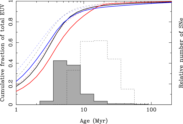
Figure 5: Output of EUV radiation for a single burst of star formation as a function of age from the BPASS models, which include prescriptions for binary stellar evolution (Eldridge & Stanway, 2009). Shown are three models, $0.1\,Z_{\odot}$ (red), $0.3\,Z_{\odot}$ (black), $Z_{\odot}$ (blue), for a stellar initial mass function of power-law slope $\alpha=-1.3$ between 0.1 and 0.5 M_⊙ and slope $\alpha=-2.35$ from 0.5 to 100 M_⊙. Dashed lines are the equivalent models with an IMF going up to 300 M_⊙. Also shown for the $0.3\,Z_{\odot}$ model are the relative numbers of type Ic supernovae (shaded histogram), and type II supernovae (dotted histogram) in each logarithmic age bin.

Although the nature of GRB progenitors remains uncertain, most scenarios suggest they are indeed likely to have lifetimes of order 5–10 Myr. For example, this is indicated by their correlation with regions of high UV emission (Larsson et al., 2007), and is roughly the range spanned by the viable single star chemically homogeneous evolution models studied by Yoon et al. (2006). To place this in context, the relative numbers of type Ic supernovae in logarithmic bins are also shown on Figure 5, and are predominantly in the range of 3 Myr to 15 Myr. Since the supernovae accompanying long-duration GRBs are also stripped-envelope events (Hjorth & Bloom, 2012), and correlate with the UV light of their hosts in a similar way (Kelly et al., 2008), it is reasonable to suppose that they span a comparable range of ages at explosion.

4.4 How representative are GRB progenitors of sources of escaping EUV radiation?

Even if GRB locations are good tracers of the dominant sources of stellar EUV radiation, it might be that they under-represent the stars from which the bulk of the escaping radiation is produced. Here we consider several such scenarios.

4.4.1 Timescales revisited - might GRBs not sample peak periods of transparency?

In Section 4.3.2 we argued that GRBs likely do explode on time-scales relevant for a significant proportion of EUV emission from a single age stellar population. However, if the peak episodes of EUV escape generally occur before the first GRBs explode following a burst of star formation, it is plausible we may not sample the relevant periods (again, for star formation of a more continuous nature, this will not be a concern).

Modelling in detail the escape of ionizing radiation from young massive stars in a range of realistic scenarios is highly challenging. On the scales of individual clouds outward pressure created by winds, radiation and supernovae competes with gravitational infall, while ionization competes with recombination. These clouds also vary in size and shape, and have complex turbulent internal structure and magnetic fields. It is also essential to incorporate the processes of star formation and evolution, which introduces further uncertainties. Finally the star forming regions exist in larger scale galactic environments. In order to escape a galaxy, radiation must first escape its local environment, likely the molecular cloud in which the stars formed, and subsequently leak out through the larger scale neutral gas distribution. Here we consider the lessons from recent state-of-the-art models which focus on different aspects of the problem.

Howard et al. (2018) examined the escape of EUV radiation from a range of massive ($10^{4}$–$10^{6}$ M_⊙) giant molecular clouds (GMCs) containing multiple massive star clusters, based on 3D simulations with ongoing star formation. They found the EUV escape from the clouds themselves to be variable in time, with occasional peaks above 10% from 2 Myr after the onset of star formation. The lower mass clouds tend to achieve high escape fractions of 20–100% by $\sim 5$ Myr, due to near complete ionization of the clouds. This is within the time-frame that some GRBs likely occur, even if the bulk of progenitors have longer lifetimes (Section 4.3.2). The intermittency here is partly the result of small-scale density structure due to the turbulent nature of the cloud, which produces time-changing local density field around the clusters. This results in a very anisotropic directional distribution of escaping radiation (something also seen in 3D models of small molecular clouds dominated by a single O star, by Walch et al., 2012). Placing these clouds into a galactic context produces galaxies with rapid (10–20 Myr) fluctuations in SFR and $f_{\rm esc}$, particularly in dwarf galaxies, with a general trend of stronger episodes of star formation being associated with lower $f_{\rm esc}$. However, these simulations did not include the effects of winds or supernovae, and also use single star stellar population prescriptions. As noted previously, inclusion of binaries is likely to increase the effectiveness of feedback, and extend the time-scales.

Rahner et al. (2017) performed 1D spherically symmetric calculations, including winds, radiative transfer and the effects of supernovae, covering a range of cloud masses, densities, star-formation efficiencies and metallicities. Here absorption is dominated by neutral gas in the swept up shell of material surrounding the central low density ionized bubble. In those models that show any appreciable EUV escape from the birth cloud at all, they also generally find a high proportion occurs during the first 2–6 Myr. Of course, these calculations are not able to include anisotropies in the shell structure, which may be key to understanding the escape fraction and, again, presumably star formation and/or EUV production more extended in time would modify these results.

Simulations that place star formation in a more cosmological context, while reliant on less sophisticated prescriptions for the feedback physics, have tended to find episodes of high escape fraction, at least in early galaxies, to have scale times of 10-20 Myr (e.g. Wise et al., 2014; Kimm & Cen, 2014; Ma et al., 2016; Trebitsch et al., 2017). This reflects timescales of star formation activity and consequent supernova feedback which has the dominant effect on the galactic scale gas distribution. Interestingly, Toy et al. (2016) suggested that GRB hosts likely have had episodic star formation, based on comparison of enrichment timescales with observed metallicities.

For comparison, star formation in the 30 Doradus H ii region (the Tarantula Nebula) in the Large Magellanic Cloud, often regarded as a local prototype of low-metallicity star-forming regions that may have been highly abundant in the early universe, has been occurring in different clumps and clusters for at least $\sim 10$ Myr (Sabbi et al., 2016). Inferring the EUV escape fraction from the Tarantula Nebula region is subject to large uncertainties, but a recent detailed study of its massive star population constrained it to be in the range 0–0.6, with a preferred value of 0.06 (Doran et al., 2013).

Clearly this is a field where much work remains to be done. It is plausible that in some circumstances, a burst of star formation in a molecular cloud towards the edge of its galaxy may lead to a brief period of high EUV escape to the IGM before the first supernovae explode. However, it does not seem likely this could be a common occurrence, and that to produce high average escape fractions would require the combined feedback effects of radiation, winds and supernovae to disperse and ionize both local and global gas, on timescales comparable to GRB progenitor lifetimes.

4.4.2 Could GRB progenitors preferentially form in higher density environments?

It has been suggested that GRBs may favour not only low metallicity, but possibly also high density sites (e.g. Kelly et al., 2014; Perley et al., 2015), for example due to dynamical processes in young dense stellar clusters being important in the formation of their progenitors (van den Heuvel & Portegies Zwart, 2013).

However, even if this is true, it is not obvious that it would significantly affect our conclusions. Very massive and dense clouds are likely to recollapse without dispersal (Rahner et al., 2017), and would also be much less affected by the GRB event itself, so GRBs forming preferentially in such environments seems to contradict the observation that only a minority of bursts are heavily dust obscured, and that absorption often is predominantly at large distances. Cases of massive GMCs where feedback does drive a strong outflow might in fact provide the best chances of creating windows of low density ionized gas to the IGM, thus favouring low column-density systems. In any event, it remains the case that GRBs occur in a range of environments, based on their galactic locations and the evidence we have of the local density, which all suggests little bias compared to the stars we expect to dominate the escaping EUV radiation.

4.4.3 Could GRB progenitors preferentially remain in higher density environments?

A sizeable fraction ($\sim 30$%) of OB stars in the Milky Way are found to have sufficiently high space velocities (several 10s of km s^-1), presumably as a result of dynamical interactions, that they will end their lives well outside their nascent birth clouds (e.g. Tetzlaff et al., 2011). Such runaway stars may sometimes spend much of their lives in relatively low density regions, and so could have a higher $\langle{f_{\rm esc}}\rangle$ than stars that remain close to their birth sites. If for some reason, such as a requirement to be a binary system, GRB progenitors were less likely to be runaways, then, on the face of it, sight-lines to GRBs would not sample that population. On the other hand, since GRBs themselves ionize gas in their locality to significant distance (see Section 4.1.2), and given that including runaways in hydrodynamic simulations only results in a modest increase of $\langle{f_{\rm esc}}\rangle$ of $\sim 20$% (Kimm & Cen, 2014), missing runaways are unlikely to have a large effect on our conclusions.

4.4.4 Could GRB progenitors create higher density sight-lines?

We can ask whether the special nature of the GRB progenitor may influence the column-densities we measure. In particular, to allow a GRB jet to reach highly relativistic velocities it is thought that their progenitors must have no extended envelope. Indeed the lack of hydrogen and helium in the spectra of supernovae accompanying GRBs confirms this picture. Expelling the envelope without also losing significant angular momentum is a potential problem for the collapsar scenario for GRB production (e.g. Detmers et al., 2008). One possibility is that high rotation could lead to chemically homogeneous evolution, essentially consuming the envelope (Yoon & Langer, 2005). Alternatively, the hydrogen and helium layers might be lost, for example through explosive common-envelope ejection in a tight binary (Podsiadlowski et al., 2010). In such cases it is plausible that the expelled material, which could amount to $\sim 10$ M_⊙, might provide enhanced absorption if it remains close enough to provide a significant column-density, but far enough not to be ionized by the ambient UV radiation field prior to the burst. Thus, even though large column-densities generally seem to be produced by gas at relatively large distance from the GRB site, it could be that a modest contribution from gas at 10–20 pc expelled by the progenitor sets an effective floor to the distribution of ${\rm log}({N_{{\text{H\,{i}}}}}/{\rm cm}^{-2})\sim 17.5$–18 in the GRB sample. Other massive stars that did not produce such high mass loss would therefore have higher escape fractions.

However, this ignores the ionizing flux of the optical flash and early afterglow of the GRBs themselves. In cases such as the two lowest column-density systems in our sample, GRBs 050908 and 060607A (Section 3.1), the bright afterglows exceeded the flux required to ionize this mass of local gas by orders of magnitude. Only if the peak UV luminosity of the burst was at least as faint as $M_{\rm AB}\approx-22$ could a proportion of the expelled gas remain neutral, and even at $z\approx 2$ this translates to a peak apparent magnitude of $m_{\rm V}\approx 23$, which is effectively unfeasible for follow-up spectroscopy with reasonable S/N given current technology. Thus, excess absorption from gas expelled by GRB progenitors can have no effect on our sample of ${N_{{\text{H\,{i}}}}}$ measurements.

4.5 Applicability to the era of reionization

As already discussed, GRBs favour low metallicity environments, and in particular appear to have a roughly constant efficiency of occurrence up to around 0.3–1 times Solar metallicity, with a rapid drop above that threshold (Cucchiara et al., 2015; Perley et al., 2016b; Graham & Fruchter, 2017; Vergani et al., 2017). This certainly suggests that GRBs should form during the EoR when few galaxies were highly metal enriched. Furthermore, known GRB hosts span a wide range in stellar mass (Perley et al., 2016b), including small, low metallicity galaxies likely representative of the galaxy populations predominant in the EoR. In particular, while three GRB hosts have now been detected by the Hubble Space Telescope (HST) at $z\sim 6$ with properties similar to those of Lyman-break galaxies at the same redshift (McGuire et al., 2016), it remains the case that the majority of GRB hosts at $z>6$ appear to be undetected to HST limits, consistent with them being drawn from a galaxy luminosity function in which the faint end dominates (Tanvir et al., 2012a; Trenti et al., 2015).

Further evidence that GRBs effectively sample stellar populations predominant in the EoR is that the rate of GRBs relative to total star formation appears to rise with redshift even faster than expected due to the metallicity sensitivity already discussed (Kistler et al., 2009; Robertson & Ellis, 2012; Perley et al., 2016b), although number statistics are small at the highest redshifts.

Thus to the extent to which analogues of EoR galaxies exist at lower redshifts, we would expect them to appear in the GRB host samples, and to be included in our column-density sample. As discussed in Section 3.3, the high-resolution cosmological simulations of galaxies at $z\sim 7$ of Cen & Kimm (2014) find that roughly half of GRBs should have ${\rm log}({N_{{\text{H\,{i}}}}}/{\rm cm}^{-2})<18$, which we certainly do not see at lower redshifts. If the prediction is correct – and limited statistics rule out a strong test at this stage – then it would require that there is a large sub-population of high-$f_{\rm esc}$ hosts at $z>6$ that barely exist in the $z<5$ host sample.

5 Discussion and Conclusions

We have compiled a large sample of H i column-density measurements obtained from GRB afterglow spectroscopy. Because GRBs select hosts over a very broad range of luminosity, we consider that they provide a good representation of the dominant populations of (not highly dusty) star forming galaxies at $z\gtrsim 2$. Despite uncertainties about the exact nature of the GRB progenitor, we also argue that the life-times and locations of GRB progenitors likely make them well suited to sampling the periods of high EUV production, and in particular the peak episodes for its escape.

Out of 138, only two sight-lines have sufficiently low column-density to allow any significant EUV to emerge. Assuming this sample is representative of the sight-lines to the massive stars dominating ionizing radiation production, we conclude an average escape fraction at the Lyman limit of $\langle{f_{\rm esc}}\rangle\approx 0.005$, with a 98% confidence upper limit of $\langle{f_{\rm esc}}\rangle\approx 0.015$. This value is in reasonable agreement with the $\langle{f_{\rm esc}}\rangle\sim 0.01$ predicted for GRB sight-lines based on the hydrodynamic simulations of Pontzen et al. (2010). It suggests that only in rare cases does stellar feedback puncture holes out of the dense ISM, providing clear windows to the IGM. This is a more stringent limit than was obtained from the recent direct search for escaping EUV at $z\approx 3.3$ by Grazian et al. (2017), who found $\langle{f_{\rm esc}}\rangle<0.017$ (67% confidence) for galaxies brighter than $L^{*}$ and $\langle{f_{\rm esc}}\rangle\lesssim 0.1$ for a sample brighter than $0.2L^{*}$.

If we account for the additional opacity due to dust for the two sight-lines for which there is any appreciable escape fraction, and the loss of highly dusty bursts from the sample altogether, then these numbers could reduce by factors of $2$–$3$. If radiation from the GRBs themselves ionized some gas in these two high-$f_{\rm esc}$ cases, then the estimate of $\langle{f_{\rm esc}}\rangle$ should be reduced further.

On the other side of the balance sheet, the difficulty of finding low column-density systems in spectra with poor signal-to-noise does provide a modest selection effect in the opposite direction. However, inspection of more complete sub-samples suggests that even missing one or two cases would be surprising, so the net effect is unlikely to be more than a factor $\sim 2$ increase in our estimate of $\langle{f_{\rm esc}}\rangle$.

The bulk of the events are at redshifts $z=2$–5, which, even accounting for these systematic uncertainties, indicates that stellar EUV falls short of providing the radiation field needed to explain the properties of the Ly$\alpha$ forest in this redshift range (Becker & Bolton, 2013; Stanway et al., 2016). More crucially, if their properties apply to galaxies during the EoR, these limits on $\langle{f_{\rm esc}}\rangle$ are at least an order of magnitude below what is required to maintain an ionized IGM in that era (Robertson et al., 2015; Stanway et al., 2016).

There is a weak suggestion of a decline in average H i column-density at the highest redshifts ($z\gtrsim 6$), but statistics remain too poor for definitive conclusions, and none of the $z>5$ sight-lines have an appreciable escape fraction. Furthermore, there is no indication of a strong correlation of neutral hydrogen column-density with either galaxy UV luminosity or stellar mass, for the subsets of our sample for which these measures are available. Thus we find no evidence to support the suggestion that ionising escape fraction may be much higher for the small galaxies that likely dominated star formation in the EoR.

Avoiding this conclusion would seem to require either that GRBs are not good tracers of the primary sources of escaping EUV, for instance because the large majority occurs before GRBs explode or because there are classes of older and less-massive stars that produce substantially more EUV than has hitherto been appreciated (e.g. as a result of binary interactions; Götberg et al., 2017), or that there is very marked evolution in the properties of GRB sight-lines between $z\sim 7$ and $z\sim 2$–5.

Overall this work shows the power of GRBs to address the difficult question of the Lyman continuum escape fraction averaged over the dominant populations of high-redshift star forming galaxies, and demonstrates the benefits of long-term campaigns to obtain GRB afterglow spectroscopy. The evidence that GRBs occur preferentially in low metallicity systems, and that their rate relative to the star formation rate increases with redshift, all suggest that they are likely good tracers of star formation in the EoR. Future samples of larger numbers of $z>6$ GRBs with good H i column-density determinations may benefit soon from the availability of JWST, and in the 2020s through the SVOM satellite working in conjunction with follow-up spectroscopy on 30-m class ground-based telescopes. Hence we may hope to obtain much tighter and more direct constraints on the contribution of stars to reionization (Yuan et al., 2016).

Appendix A Individual bursts

In this appendix we provide information about selected GRBs. In particular we present our Ly$\alpha$ fits for those cases where the column-densities have not previously been reported and are not included in Selsing et al. (2018). Unless stated otherwise, the precise redshift is taken from metal absorption lines seen in the spectra, which reduces the free parameters, and improves accuracy of the fits. Details of the fitting procedure are given in Selsing et al. (2018).

We caution that the nature of target-of-opportunity observations of variable sources means that the source magnitude is frequently poorly known prior to observation, in many cases there was limited time available, and non-optimal conditions or sky location. Thus, some of the spectra are unusually low signal-to-noise and/or suffer from imperfect flux calibration or other anomalies. Furthermore, there are cases where host galaxy emission, including Ly$\alpha$ emission lines, contaminates the afterglow signal, and where intervening absorbers introduce metal lines. However, fortunately for the purposes of this analysis, the red-wing of the Ly$\alpha$ absorption features can still be measured to an adequate level of precision, with little overall systematic bias in determination of ${N_{{\text{H\,{i}}}}}$.

Data are taken from various sources: some from observations we obtained ourselves and in other cases from archives. Spectrographs used include the Gemini Multi-Object Spectrograph North and South (GMOS-N, GMOS-S), the VLT FOcal Reducer and low dispersion Spectrograph (FORS1 and FORS2) and UltraViolet Echelle Spectrograph (UVES), the William Herschel Telescope (WHT) Intermediate dispersion Spectrograph and Imaging System (ISIS) and Auxiliary port CAMera (ACAM), the Gran Telescopio Canarias (GTC) Optical System for Imaging and low-Intermediate-Resolution Integrated Spectroscopy (OSIRIS), the Nordic Optical Telescope (NOT) Andalucia Faint Object Spectrograph and Camera (ALFOSC), the Telescopio Nazionale Galileo (TNG) Device Optimized for the Low Resolution (DOLoRes), the Asiago Copernico Telescope (CT) Asiago Faint Object Spectrograph and Camera (AFOSC), the Keck Low Resolution Imaging Spectrograph (LRIS).

Spectra presented in this appendix will be made available in the GRBspec database http://grbspec.iaa.es (de Ugarte Postigo et al., 2014a).

A.1 GRB 021004

The bright afterglow of GRB 021004 was well studied, and spectroscopy revealed an unusually complex velocity structure for the absorbing gas (Fiore et al., 2005; Starling et al., 2005; Castro-Tirado et al., 2010). Combined with saturation of the lines, establishing the H i column-density was not straight-forward, and here we adopt a reasonable value and error based on the ${\rm log}({N_{{\text{H\,{i}}}}}/{\rm cm}^{-2})>18$ from the the absence of continuum below the Lyman limit (Fynbo et al., 2005) and ${\rm log}({N_{{\text{H\,{i}}}}}/{\rm cm}^{-2})<20$ from analysis of the multiple Ly$\alpha$ lines themselves (Møller et al., 2002).

A.2 GRB 060522

GRB 060522 was observed with Keck-I/LRIS, starting 14:24 UT on 22-May-2006. A total exposure of $1800$ s was obtained. The fit to the Ly$\alpha$ line is shown in Figure 6; the inferred column ${\rm log}({N_{{\text{H\,{i}}}}}/{\rm cm}^{-2})=20.6\pm 0.3$ is consistent with previous estimates (Cenko et al., 2006; Chary et al., 2007). Note, the region redward of Ly$\alpha$ is badly affected by fringing, impeding searches for metal absorption lines.

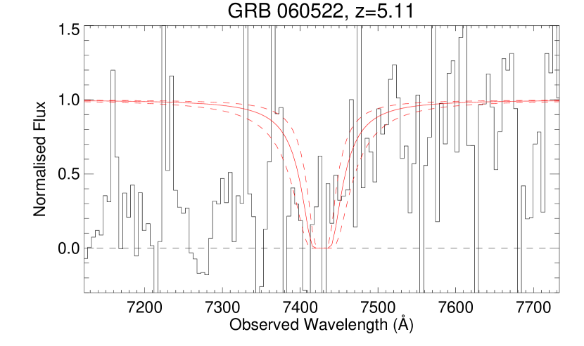
Figure 6: Fit of the red wing of Ly$\alpha$ for the GRB 060522 Keck-I/LRIS spectrum.

A.3 GRB 070223

Near-IR imaging of GRB 070223 was obtained with the WHT Long-slit Intermediate Resolution Infrared Spectrograph (LIRIS) instrument in the $JHK$ filters between 2.7 and 3.7 hr post-burst. A faint source was detected at the location of the X-ray afterglow (Rol et al., 2007), for which we find a magnitude $K_{\rm AB}=21.9\pm 0.3$ calibrated against 2MASS stars in the field (and corrected for small foreground extinction via Schlafly & Finkbeiner, 2011). Subsequent imaging obtained 8 day post-burst showed this source to have declined to $K_{\rm AB}=22.8\pm 0.2$, confirming the identification of the afterglow, but also indicating the presence of an underlying host galaxy (also detected in 3.6 $\mu$m Spitzer imaging by Perley et al., 2016b).

GRB 070223 was observed rapidly with the 2 m Liverpool Telescope (LT) in various optical filters, beginning only 18 min post-burst (Melandri et al., 2008). We created a 30 min stacked integration from $r$-band imaging taken between 3 and 3.7 hr post-burst. At the location of the $K$-band transient, there is a faint detection of a source with foreground corrected magnitude $r=23.8\pm 0.3$, calibrated against SDSS stars in the field. This object was also seen in $R$-band early imaging by the MDM 1.3 m telescope (Rol et al., 2007), but, as detailed in the text, appears to be a constant source, presumably the host galaxy.

A.4 GRB 070810A

GRB 070810A was observed with Keck-I/LRIS, starting 05:47 UT on 10-Aug-2007. A total exposure of $2\times 600$ s was obtained (Thöne et al., 2007). The fit to the Ly$\alpha$ line is shown in Figure 7.

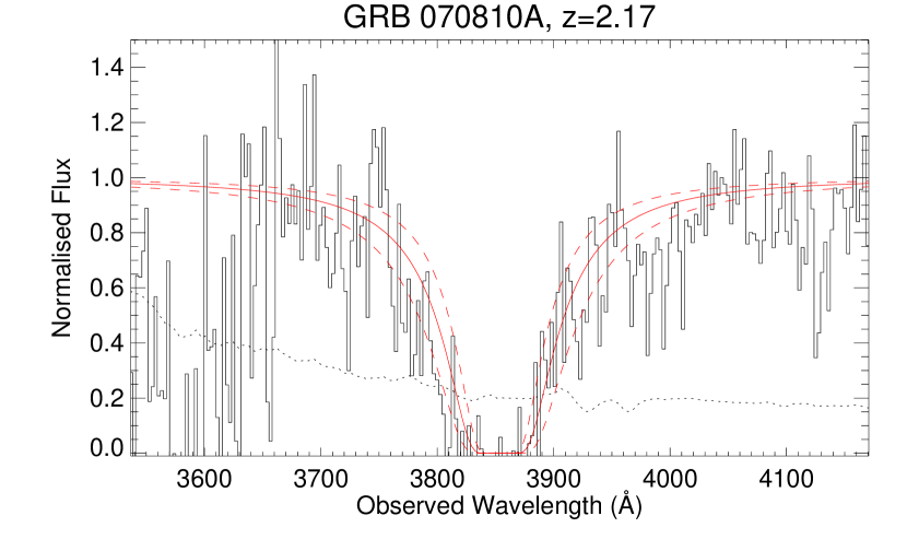
Figure 7: Fit of the red wing of Ly$\alpha$ for the GRB 070810A Keck-I/LRIS spectrum.

A.5 GRB 080129

GRB 080129 was observed with VLT/FORS1, starting 05:24 UT on 30-Jan-2008. A total exposure of $4\times 1800$ s was obtained with the OG590 blocking filter and 300I grism, and reduced with the standard ESO pipeline (Greiner et al., 2009b). The redshift is fixed to that of the metal absorption lines, and the fit to the red wing of Ly$\alpha$ (Figure 8) is rather poor in this case, plausibly due to velocity structure in low metallicity and low column-density gas close to the host.

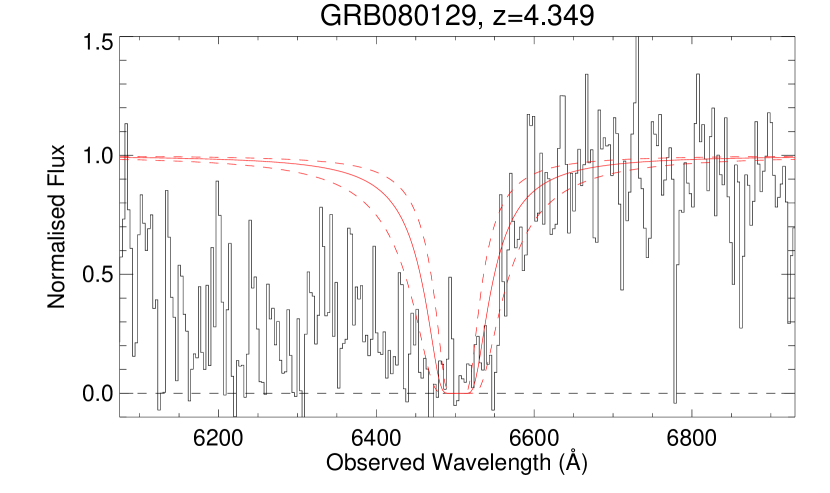
Figure 8: Fit of the red wing of Ly$\alpha$ for the GRB 080129 VLT/FORS1 spectrum.

A.6 GRB 080810

GRB 080810 was observed at high resolution by Keck/HIRES (Prochaska et al., 2008), and the spectrum showed a somewhat complex H i absorption system, with two main components separated by $\approx 700$ km s^-1. The lower redshift system showed Si ii* fine-structure lines, suggesting this gas was closer to the GRB location, and likely that the other system is infalling on the near-side. Page et al. (2009) found an upper limit for the combined absorber of ${\rm log}({N_{{\text{H\,{i}}}}}/{\rm cm}^{-2})<19.5$ and a lower limit for the higher redshift component of ${\rm log}({N_{{\text{H\,{i}}}}}/{\rm cm}^{-2})>17.7$ from the absence of emission below the Lyman limit. Recently, Wiseman et al. (2017) reanalysed the HIRES spectrum, finding ${\rm log}({N_{{\text{H\,{i}}}}}/{\rm cm}^{-2})=18.10\pm 0.25$ for this dominant component, which we use here.

A.7 GRB 080905B

GRB 080905B was observed by VLT/FORS2, starting 01:16 UT on 6-Sep-2008. A total exposure of $2\times 600$ s was obtained with the GRIS_300V grism, and reduced with the standard ESO pipeline (Vreeswijk et al., 2008). The fit to the Ly$\alpha$ line is shown in Figure 9.

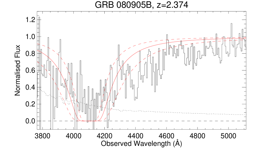
Figure 9: Fit of the red wing of Ly$\alpha$ for the GRB 080905B VLT/FORS2 spectrum.

A.8 GRB 080913

GRB 080913 was observed with VLT/FORS2, being found to be at redshift $z\approx 6.7$ from the location of the Ly$\alpha$ break by Greiner et al. (2009a). Lacking a precise metal line redshift, Greiner et al. (2009a) were only able to place weak constraints on the H i column-density concluding $20.3<{\rm log}({N_{{\text{H\,{i}}}}}/{\rm cm}^{-2})<21.4$. A subsequent reanalysis of the spectrum by Patel et al. (2010) located a weak S ii+Si ii blend, establishing a firmer redshift of $z=6.733$. This allowed a more precise determination of the H i column-density, ${\rm log}({N_{{\text{H\,{i}}}}}/{\rm cm}^{-2})=19.84$ assuming no neutral component of the IGM, and ${\rm log}({N_{{\text{H\,{i}}}}}/{\rm cm}^{-2})=19.6$ in a fit that allowed the neutral fraction of the IGM to be a free parameter (specifically they found $x_{{\text{H\,{i}}}}=0.06$). Given this uncertainty, and the poor S/N of the spectrum, we adopt ${\rm log}({N_{{\text{H\,{i}}}}}/{\rm cm}^{-2})=19.6\pm 0.3$ here.

A.9 GRB 081029

GRB 081029 was observed by Gemini/GMOS-S, starting 07:04 UT on 29-Oct-2008 (Cucchiara et al., 2008a). A total exposure of $2\times 900$ s was obtained with the R400 grating set at 6000 Å central wavelength and reduced using the standard Gemini reduction tools within Iraf. The fit to the Ly$\alpha$ line is shown in Figure 10.

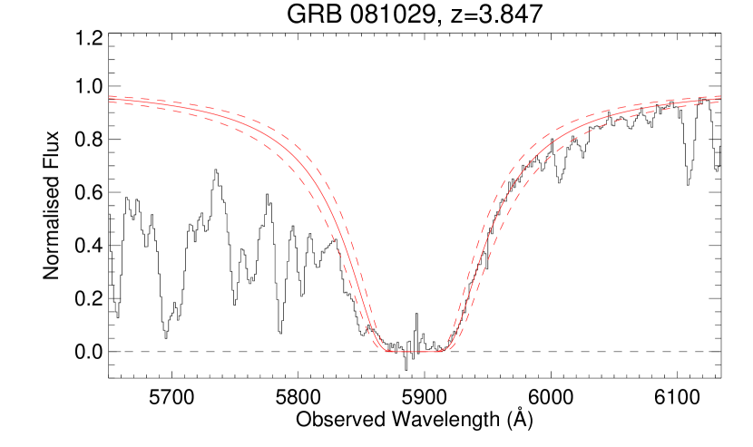
Figure 10: Fit of the red wing of Ly$\alpha$ for the GRB 081029 Gemini/GMOS-S spectrum.

A.10 GRB 081118

GRB 081118 was observed by VLT/FORS2, starting 02:48 UT on 19-Nov-2008. A total exposure of $2\times 1800$ s was obtained with the GRIS_300V grism, and reduced with the standard ESO pipeline (D’Elia et al., 2008). The fit to the Ly$\alpha$ line is shown in Figure 11.

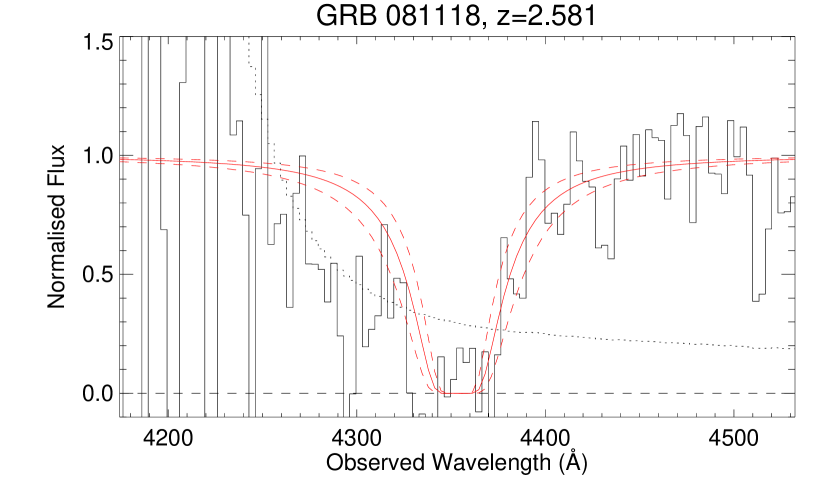
Figure 11: Fit of the red wing of Ly$\alpha$ for the GRB 081118 VLT/FORS2 spectrum.

A.11 GRB 081222

GRB 081222 was observed by Gemini/GMOS-S, starting 01:02 UT on 23-Dec-2008 (Cucchiara et al., 2008b). A total exposure of $2\times 900$ s was obtained with the R400 grating set at 6000 Å central wavelength, and reduced using the standard Gemini reduction tools within Iraf. The fit to the Ly$\alpha$ line is shown in Figure 12.

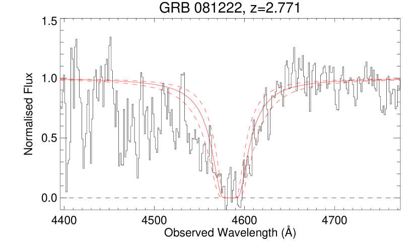
Figure 12: Fit of the red wing of Ly$\alpha$ for the GRB 081222 Gemini/GMOS-S spectrum.

A.12 GRB 090313

GRB 090313 was observed by Gemini/GMOS-S, starting 04:20 UT on 14-Mar-2009 (Chornock et al., 2009a). A total exposure of $2\times 600$ s was obtained with the R400 grating set at 6000 Å central wavelength, and reduced using the standard Gemini reduction tools within Iraf. The fit to the Ly$\alpha$ line is shown in Figure 13.

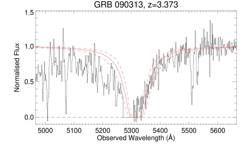
Figure 13: Fit of the red wing of Ly$\alpha$ for the GRB 090313 Gemini/GMOS-S spectrum. Note that there is a gap between chips of the camera around 5280 Å. This produces an anomaly in the trace which was ignored in the fit.

A.13 GRB 090323

GRB 090323 was unusual exhibiting two absorption systems separated by $\approx 700$ km s^-1, and a relatively high metal abundance (Savaglio et al., 2012). In this case both systems showed Si ii* fine structure lines, likely indicating fairly close proximity to the GRB. The value for ${N_{{\text{H\,{i}}}}}$ used here was obtained by summing the column-densities of the two systems.

A.14 GRB 090426

The prompt duration of GRB 090426 was $T_{90}\approx 1.3$ s, suggesting it could be a short-duration burst, particularly given that cosmological time-dilation makes this less than 0.4 s in the source-frame. However since it was intrinsically bright and took place in an interacting star-forming system (Thöne et al., 2011), we include it in our sample as a possible long-duration GRB (see also Nicuesa Guelbenzu et al., 2011). The H i column-density in this case was seen to vary, and we take here that measured at 1.1 hr post-burst by Levesque et al. (2010a) using Keck/LRIS. Removing GRB 090426 from the sample would not have a significant affect on any of the conclusions.

A.15 GRB 090519

GRB 090519 was observed by VLT/FORS2 starting at 01:03 on 20-May-2009 UT (Thoene et al., 2009). A total exposure of $3\times 1800$ s was obtained, covering the wavelength range 3500–9200Å. The fit to the Ly$\alpha$ line is shown in Figure 14. The afterglow was faint, and the redshift is estimated from the Ly$\alpha$ and Ly$\beta$ breaks since no clear metal lines were seen.

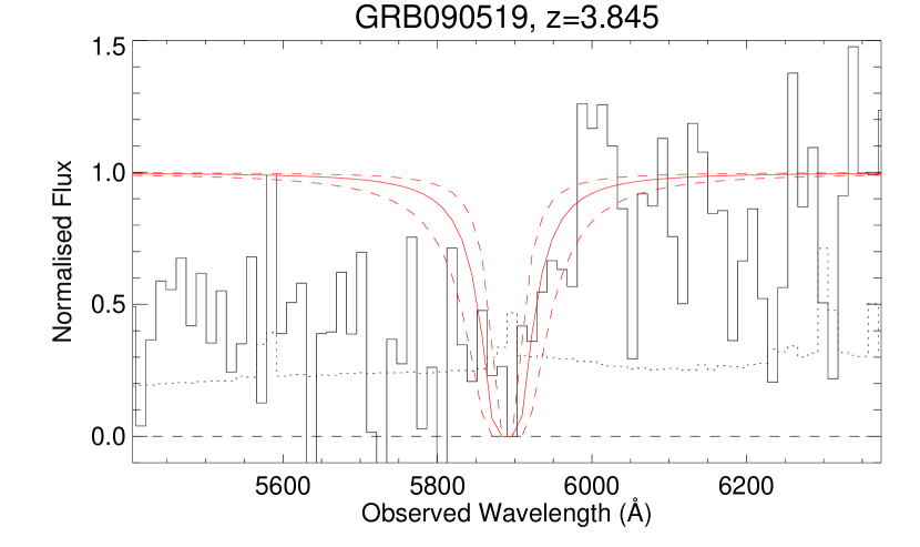
Figure 14: Fit of the red wing of Ly$\alpha$ for the GRB 090519 VLT/FORS2 spectrum.

A.16 GRB 090529

GRB 090529 was observed by VLT/FORS2 starting at 01:52 on 31-May-2009 UT, roughly 1.5 days post-burst (Malesani et al., 2009). A total exposure of $2\times 1800$ s was obtained, covering the wavelength range 3500–9200Å. The fit to the Ly$\alpha$ line is shown in Figure 15. Although the S/N is unusually poor (largely due to the lateness of the observation), the fit benefits from the redshift being fixed by metal absorption lines.

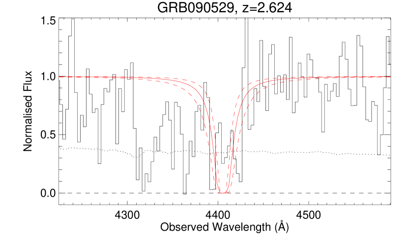
Figure 15: Fit of the red wing of Ly$\alpha$ for the GRB 090529 VLT/FORS2 spectrum.

A.17 GRB 090715B

GRB 090715B was observed with the WHT/ISIS starting 23:46 UT on 15-Jul-2009 (Wiersema et al., 2009). This spectrograph has a blue and a red arm, separated by a dichroic; we used the 300B and 316R gratings. Spectroscopic observations consisted of $4\times 900$ s exposure time. The data were reduced using standard techniques in IRAF. Several metal absorption lines give a redshift $z=3.01$. The fit to the Ly$\alpha$ line is shown in Figure 16.

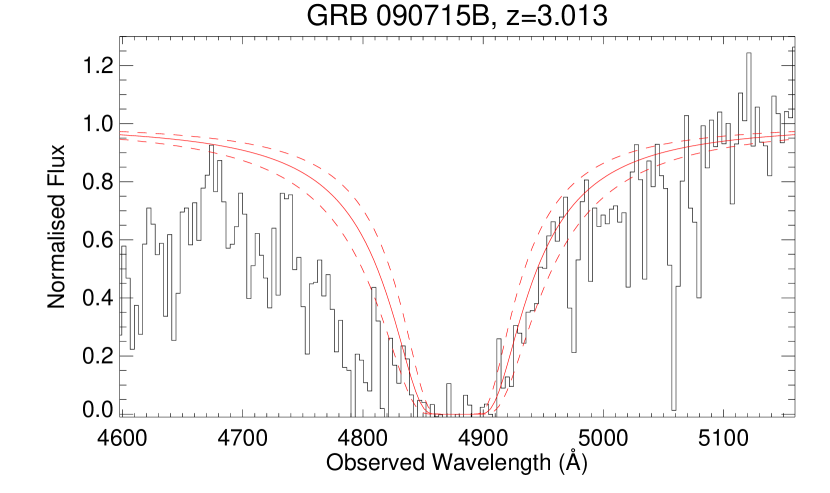
Figure 16: Fit of the red wing of Ly$\alpha$ for the GRB 090715B WHT/ISIS spectrum.

A.18 GRB 090726

GRB 090726 was observed by the SAO RAS 6-m telescope using the SCORPIO spectrograph starting at 00:15 on 27-Jul-2009 UT (Fatkhullin et al., 2009). A total exposure of $600$ s was obtained, covering the wavelength range 3700–7800Å. The fit to the Ly$\alpha$ line is shown in Figure 17.

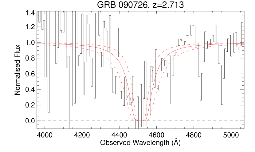
Figure 17: Fit of the red wing of Ly$\alpha$ for the GRB 090726 SAO RAS 6-m / SCORPIO spectrum.

A.19 GRB 091029

GRB 091029 was observed by Gemini/GMOS-S, starting 06:05 UT on 29-Oct-2009 (Chornock et al., 2009b). A total exposure of $4\times 600$ s was obtained with the R400 grating set at 6000 Å central wavelength and reduced using the standard Gemini reduction tools within Iraf. The fit to the Ly$\alpha$ line is shown in Figure 18.

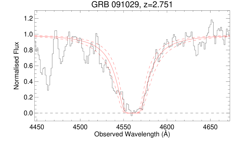
Figure 18: Fit of the red wing of Ly$\alpha$ for the GRB 091029 Gemini/GMOS-S spectrum.

A.20 GRB 100302A

GRB 100302A was observed by Gemini/GMOS-N, starting 09:42 UT on 03-Mar-2010 (Chornock et al., 2010). A total exposure of $1200$ s was obtained with the R400 grating. The continuum S/N is rather poor, but weak metal lines indicate a redshift of $z=4.813$. The fit to the Ly$\alpha$ red wing is shown in Figure 19.

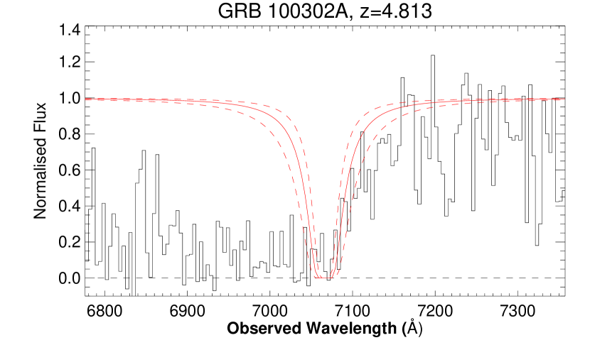
Figure 19: Fit of the red wing of Ly$\alpha$ for the GRB 100302A Gemini/GMOS spectrum.

A.21 GRB 100316A

GRB 100316A was observed by GTC/OSIRIS, starting 06:13 UT on 16-Mar-2010 (Sánchez-Ramírez et al., 2013a). A total exposure of $2\times 900$ s was obtained with the R300B grating. The fit to the Ly$\alpha$ line is shown in Figure 20. The precise redshift is known from the Ly$\alpha$  emission line in a late-time spectrum of the host.

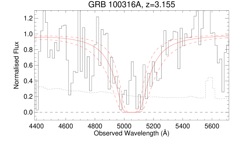
Figure 20: Fit of the red wing of Ly$\alpha$ for the GRB 100316A GTC/OSIRIS spectrum. Ly$\alpha$ line emission from the host galaxy is evident in the absorption trough, but does not affect the fit.

A.22 GRB 100513A

GRB 100513A was observed by Gemini/GMOS-N, starting 06:13 UT on 13-May-2010 (Cenko et al., 2010). A total exposure of $2\times 1200$ s was obtained with the R400 grating set at 8000 Å central wavelength and reduced using the standard Gemini reduction tools within Iraf. The fit to the Ly$\alpha$ line is shown in Figure 21.

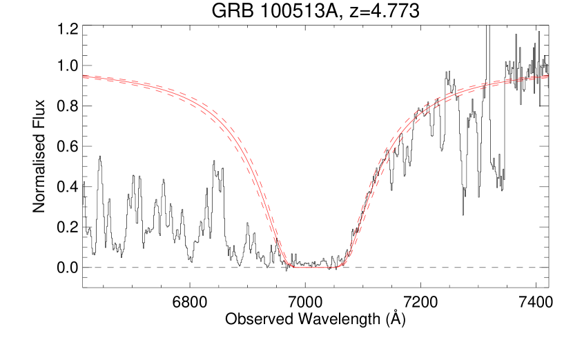
Figure 21: Fit of the red wing of Ly$\alpha$ for the GRB 100513A Gemini/GMOS-N spectrum. The large dips redward of the Ly$\alpha$ line are residuals due to gaps between the detectors in the spectrograph.

A.23 GRB 110731A

GRB 110731A was observed by Gemini/GMOS-N, starting 09:08 UT on 01-Aug-2011 (Tanvir et al., 2011). A total exposure of $4\times 900$ s was obtained with the B600 grating set at 5250 Å central wavelength and reduced using the standard Gemini reduction tools within Iraf. The fit to the Ly$\alpha$ line is shown in Figure 22.

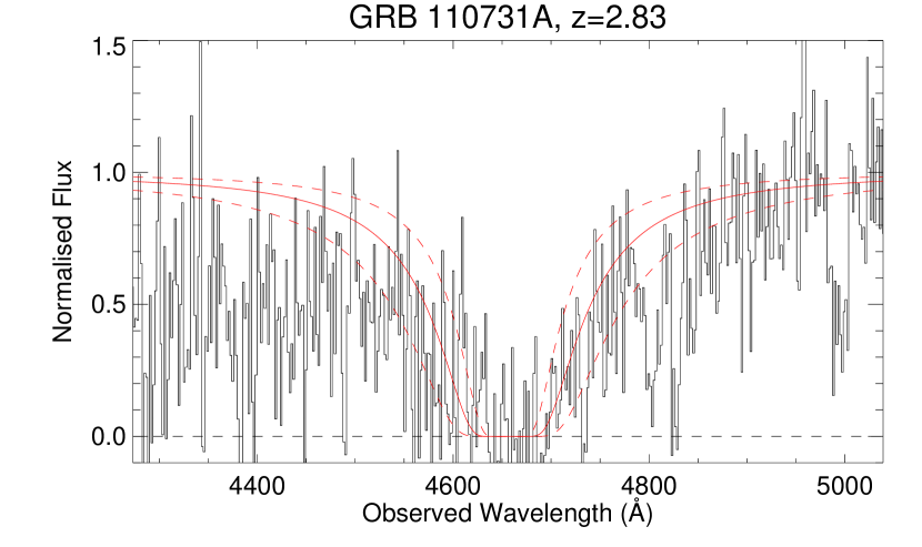
Figure 22: Fit of the red wing of Ly$\alpha$ for the GRB 110731A Gemini/GMOS-N spectrum. The apparent feature at 4800 Å is due to the gap between the detectors in the spectrograph.

A.24 GRB 120811C

GRB 120811C was observed by the GTC/OSIRIS, starting 15:35 UT on 11-Aug-2012 (Thöne et al., 2012). A total exposure time of 2400 s was obtained, spanning a wavelength range 3640–7875 Å. The fit to the Ly$\alpha$ line is shown in Figure 23.

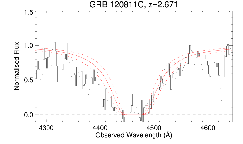
Figure 23: Fit of the red wing of Ly$\alpha$ for the GRB 120811C GTC/OSIRIS spectrum.

A.25 GRB 121027A

GRB 121027A has been suggested as a member of the ‘ultra-long’ class of GRBs, whose exact nature remains uncertain, but since they also appear to be associated with massive stars in low metallicity galaxies (Levan et al., 2014; Greiner et al., 2015a; Kann et al., 2017), we include it in our sample.

A.26 GRB 121128A

GRB 121128A was observed by Gemini/GMOS-N, starting 06:28 UT on 28-Nov-2012 (Tanvir et al., 2012b). A total exposure of $4\times 400$ s was obtained with the B600 grating set at 5250 Å central wavelength and reduced using the standard Gemini reduction tools within Iraf. The fit to the Ly$\alpha$ line is shown in Figure 24.

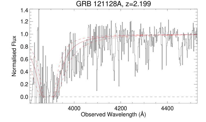
Figure 24: Fit of the red wing of Ly$\alpha$ for the GRB 121128A Gemini/GMOS-N spectrum.

A.27 GRB 130518A

GRB 130518A was observed at high resolution with GTC/OSIRIS, starting 04:47 UT on 20-May-2013. A total exposure time of 840 s was obtained, spanning a wavelength range 3700–7800 Å and was originally reported in Sanchez-Ramirez et al. (2013b). The fit to the Ly$\alpha$ line is shown in Figure 25.

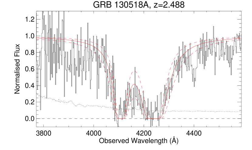
Figure 25: Fit of the red wing of Ly$\alpha$ for the GRB 130518A GTC/OSIRIS spectrum. A second, intervening DLA, at $z=2.38$ is apparent.

A.28 GRB 130610A

GRB 130610A was observed at high resolution with VLT/UVES, starting 03:25 UT on 10-Jun-2013 (Smette et al., 2013). A series of exposures were obtained totalling 6500 s. The fit to the Ly$\alpha$ line is shown in Figure 26.

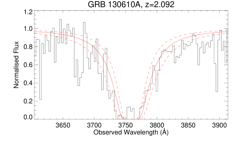
Figure 26: Fit of the red wing of Ly$\alpha$ for the GRB 130610A VLT/UVES spectrum.

A.29 GRB 131108A

GRB 131108A was observed with the GTC/OSIRIS, starting 20:42 UT on 08-Nov-2013 (de Ugarte Postigo et al., 2013). A total exposure of 1800 s was obtained covering a spectral range 3700–7870 Å. The fit to the Ly$\alpha$ line is shown in Figure 27.

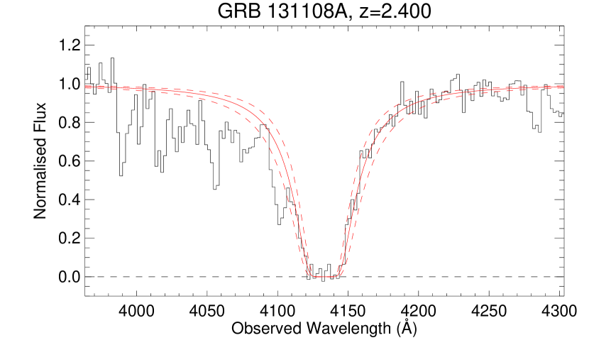
Figure 27: Fit of the red wing of Ly$\alpha$ for the GRB 131108A GTC/OSIRIS spectrum.

A.30 GRB 140206A

GRB 140206A was observed with the NOT/ALFOSC starting 19:56 UT on 6-Feb-2014 (Malesani et al., 2014, see also D’Elia et al. (2014) for TNG/DOLoRes spectroscopy). A total exposure of 3600 s was obtained covering a spectral range 3750–9000 Å. The fit to the Ly$\alpha$ line is shown in Figure 28.

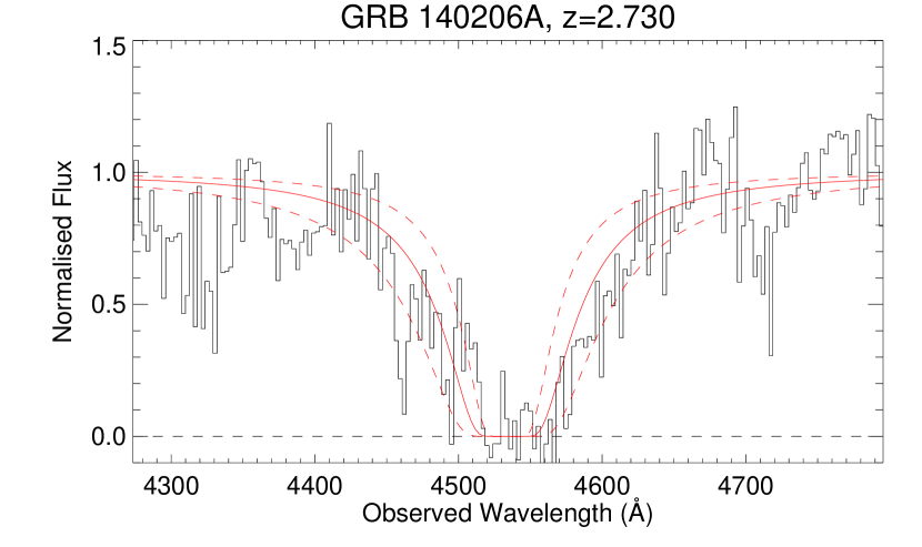
Figure 28: Fit of the red wing of Ly$\alpha$ for the GRB 140206A NOT/ALFOSC spectrum.

A.31 GRB 140515A

GRB 140515A was a high redshift burst observed at several facilities. No metal lines were confidently detected so the redshift could only be estimated from the Ly$\alpha$ break itself. This limits the conclusions that can be drawn, since the damping wing must be decomposed into ISM and IGM contributions, which is less certain in the absence of a precise redshift. Nonetheless, the sharpness of the break clearly indicates a relatively low H i column-density. Chornock et al. (2014) obtained a value of ${\rm log}({N_{{\text{H\,{i}}}}}/{\rm cm}^{-2})=18.62\pm 0.08$ assuming an ionized IGM and ${\rm log}({N_{{\text{H\,{i}}}}}/{\rm cm}^{-2})=18.43$ in a joint fit including a neutral IGM component from an early Gemini-N/GMOS spectrum. Melandri et al. (2015) analysed later GTC and VLT spectroscopy and concluded ${\rm log}({N_{{\text{H\,{i}}}}}/{\rm cm}^{-2})<18.5$ whereas Selsing et al. (2018) estimate ${\rm log}({N_{{\text{H\,{i}}}}}/{\rm cm}^{-2})=19.0\pm 0.5$. In this paper we therefore adopt a compromise value of ${\rm log}({N_{{\text{H\,{i}}}}}/{\rm cm}^{-2})=18.5\pm 0.3$.

A.32 GRB 140629A

GRB 140629A was observed with the TNG/DOLoRes, starting 02:07 UT on 30-Jun-2014 (D’Avanzo et al., 2014). A total exposure of 1200 s was obtained, covering a spectral range 3000–8000 Å. The fit to the Ly$\alpha$ line is shown in Figure 29.

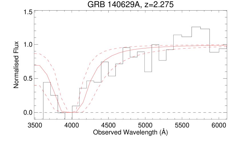
Figure 29: Fit of the red wing of Ly$\alpha$ for the GRB 140629A TNG/DOLoRes spectrum.

A.33 GRB 140703A

GRB 140703A was observed with the GTC/OSIRIS, starting 03:16 UT on 3-Jul-2014. A total exposure of 450 s was obtained covering a spectral range 3700–10000 Å and was originally reported in Castro-Tirado et al. (2014). The fit to the Ly$\alpha$ line is shown in Figure 30.

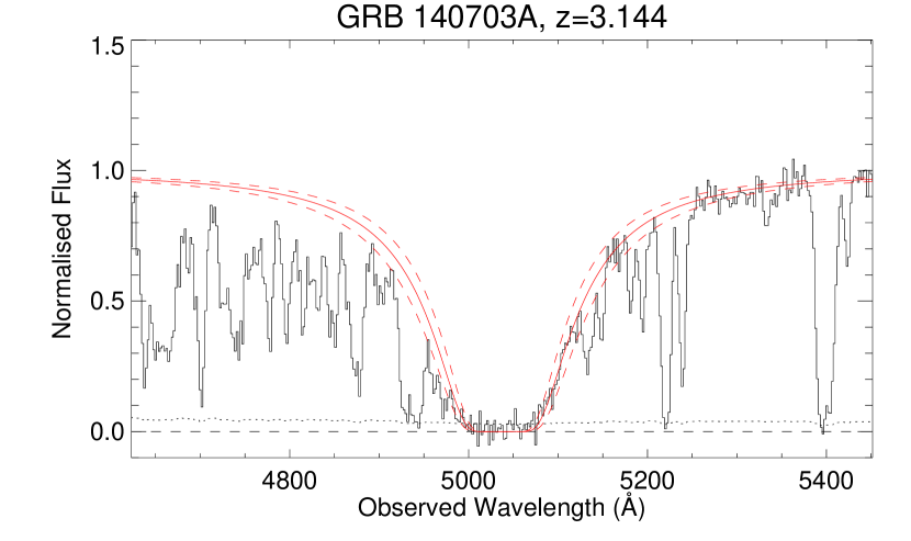
Figure 30: Fit of the red wing of Ly$\alpha$ for the GRB 140703A GTC/OSIRIS spectrum.

A.34 GRB 140808A

GRB 140808A was observed with the GTC/OSIRIS, starting 00:54 UT on 08-Aug-2014 (Gorosabel et al., 2014). A total exposure of 3600 s was obtained covering a spectral range 3700–7800 Å. The fit to the Ly$\alpha$ line is shown in Figure 31.

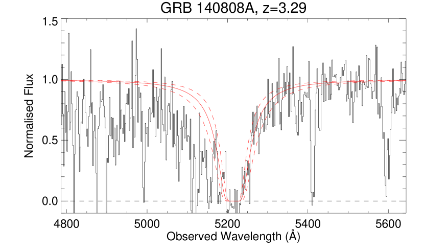
Figure 31: Fit of the red wing of Ly$\alpha$ for the GRB 140808A GTC/OSIRIS spectrum.

A.35 GRB 150413A

GRB 150413A was observed with the Asiago(CT)/AFOSC, starting 20:53 UT on 13-Apr-2015 (de Ugarte Postigo & Tomasella, 2015). A total exposure of 1800 s was obtained covering a wavelength range 3400–8200 Å. The fit to the Ly$\alpha$ line is shown in Figure 32.

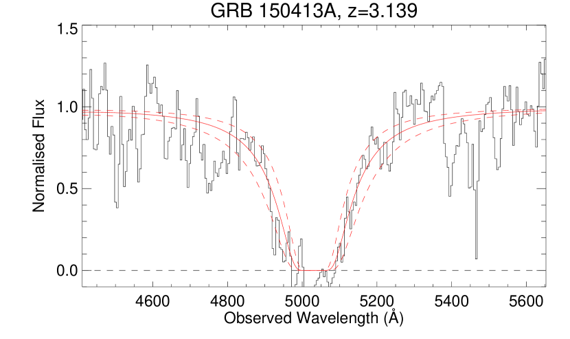
Figure 32: Fit of the red wing of Ly$\alpha$ for the GRB 150413A CT/AFOSC spectrum.

A.36 GRB 151215A

GRB 151215A was observed with the NOT/ALFOSC, starting 04:13 UT on 15-Dec-2015 (Xu et al., 2015). A total exposure of $3\times 1200$ s was obtained covering a spectral range 3200–9000 Å. The fit to the Ly$\alpha$ line is shown in Figure 33.

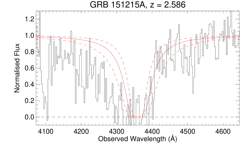
Figure 33: Fit of the red wing of Ly$\alpha$ for the GRB 151215A NOT/ALFOSC spectrum.

A.37 GRB 160227A

GRB 160227A was observed with the NOT/ALFOSC, starting at 20:19 UT on 27-Feb-2016 (Xu et al., 2016b). A total exposure of 4800 s was obtained covering a wavelength range 3200–9000 Å. The fit to the Ly$\alpha$ line is shown in Figure 34.

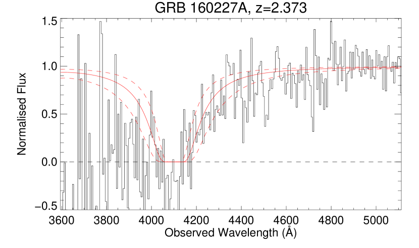
Figure 34: Fit of the red wing of Ly$\alpha$ for the GRB 160227A NOT/ALFOSC spectrum.

A.38 GRB 160629A

GRB 160629A was observed with the GTC/OSIRIS, starting at 04:40 UT on 30-Jun-2016 (Castro-Tirado et al., 2016). A total exposure of 600 s was obtained covering a wavelength range 3700–7880 Å. The fit to the Ly$\alpha$ line is shown in Figure 35.

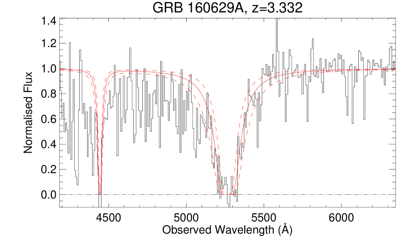
Figure 35: Fit of the red wing of Ly$\alpha$ for the GRB 160629A GTC/OSIRIS spectrum.

A.39 GRB 161017A

GRB 161017A was observed with the TNG/DOLoRes, starting at 04:27 UT on 18-Oct-2016 (D’Avanzo et al., 2016). A total exposure of 1200 s was obtained covering a wavelength range 3500–8000 Å. The fit to the Ly$\alpha$ line is shown in Figure 36.

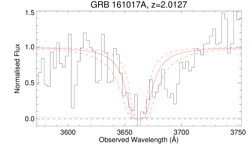
Figure 36: Fit of the red wing of Ly$\alpha$ for the GRB 161017A TNG/DOLoRes spectrum.

For this GRB we also conducted a host search using the WHT/ACAM on 7 April 2017. In seeing of 1.1 arcsec we obtained a 45 min integration in the $g$-band. No source was detected at the GRB position down to a 2$\sigma$ limiting magnitude of $g=24.70$, which is corrected for foreground Milky Way extinction (Schlafly & Finkbeiner, 2011).

A.40 GRB 170405A

GRB 170405A was observed with the GTC/OSIRIS, starting at 02:14 UT on 6-Apr-2017 (de Ugarte Postigo et al., 2017a). A total exposure of $3\times 900$ s was obtained covering a wavelength range 3700–7800 Å. The fit to the Ly$\alpha$ line is shown in Figure 37.

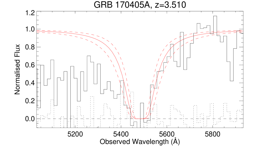
Figure 37: Fit of the red wing of Ly$\alpha$ for the GRB 170405A GTC/OSIRIS spectrum.

A.41 GRB 170531B

GRB 170531B was observed with the GTC/OSIRIS, starting at 02:47 UT on 1-Jun-2017 (de Ugarte Postigo et al., 2017b). A total exposure of $3\times 900$ s was obtained covering a wavelength range 3700–7880 Å. The fit to the Ly$\alpha$ line is shown in Figure 38.

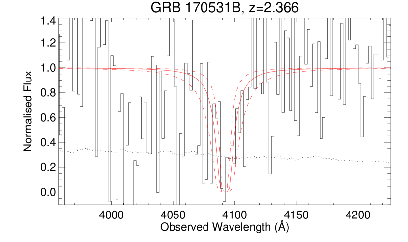
Figure 38: Fit of the red wing of Ly$\alpha$ for the GRB 170531B GTC/OSIRIS spectrum.

A.42 GRB 180115A

GRB 180115A was observed with the GTC/OSIRIS, starting at 20:32 UT on 15-Jan-2018 (de Ugarte Postigo et al., 2018). A total exposure of $3\times 900$ s was obtained covering a wavelength range 3700–7880 Å. The fit to the Ly$\alpha$ line is shown in Figure 39. In this case, no metal lines were detected, so the redshift is based solely on Ly$\alpha$.

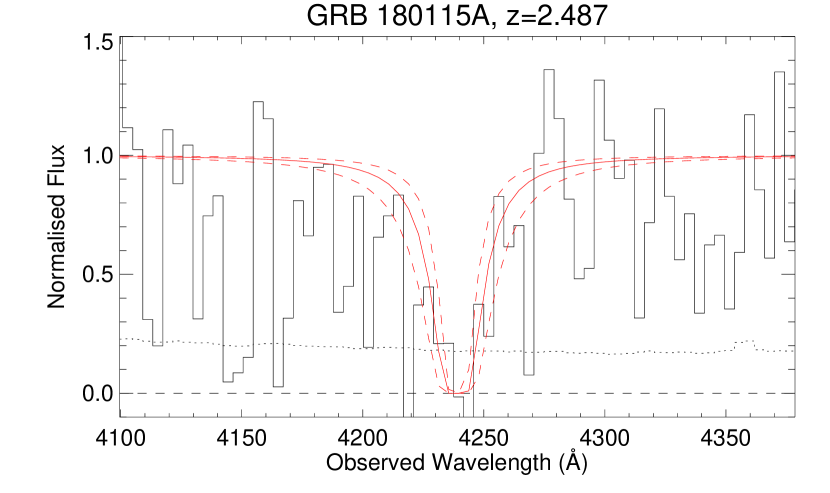
Figure 39: Fit of the red wing of Ly$\alpha$ for the GRB 180115A GTC/OSIRIS spectrum.

A.43 GRB 180329B

GRB 180329B was observed with the VLT/X-shooter, starting at 00:10 UT on 30-Mar-2018 (Izzo et al., 2018). A total exposure of $2\times 600$ s was obtained covering a wavelength range 3000–21000 Å. The fit to the Ly$\alpha$ line is shown in Figure 40.

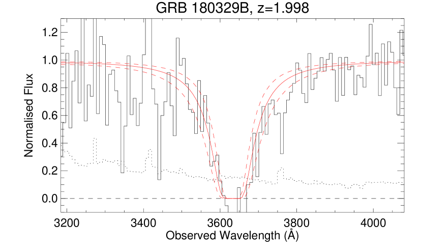
Figure 40: Fit of the red wing of Ly$\alpha$ for the GRB 180329B VLT/X-shooter spectrum.

References

- Anderson et al. (2012) Anderson J. P., Habergham S. M., James P. A., Hamuy M., 2012, MNRAS, 424, 1372
- Anderson et al. (2017) Anderson L., Governato F., Karcher M., Quinn T., Wadsley J., 2017, MNRAS, 468, 4077
- Becker & Bolton (2013) Becker G. D., Bolton J. S., 2013, MNRAS, 436, 1023
- Berger et al. (2006) Berger E., Penprase B. E., Cenko S. B., Kulkarni S. R., Fox D. B., Steidel C. C., Reddy N. A., 2006, ApJ, 642, 979
- Blanchard et al. (2016) Blanchard P. K., Berger E., Fong W.-f., 2016, ApJ, 817, 144
- Bolmer et al. (2018) Bolmer J., Greiner J., Krühler T., Schady P., Ledoux C., Tanvir N. R., Levan A. J., 2018, A&A, 609, A62
- Bouchet et al. (1985) Bouchet P., Lequeux J., Maurice E., Prevot L., Prevot-Burnichon M. L., 1985, A&A, 149, 330
- Bouwens et al. (2012) Bouwens R. J., et al., 2012, ApJ, 752, L5
- Camps-Fariña et al. (2017) Camps-Fariña A., Zaragoza-Cardiel J., Beckman J. E., Font J., Velázquez P. F., Rodríguez-González A., Rosado M., 2017, MNRAS, 468, 4134
- Castro-Tirado et al. (2010) Castro-Tirado A. J., et al., 2010, A&A, 517, A61
- Castro-Tirado et al. (2014) Castro-Tirado A. J., et al., 2014, GRB Coordinates Network, 16505
- Castro-Tirado et al. (2016) Castro-Tirado A. J., et al., 2016, GRB Coordinates Network, 19632
- Cen & Kimm (2014) Cen R., Kimm T., 2014, ApJ, 794, 50
- Cenko et al. (2006) Cenko S. B., Berger E., Djorgovski S. G., Mahabal A. A., Fox D. B., 2006, GRB Coordinates Network, 5155
- Cenko et al. (2008) Cenko S. B., et al., 2008, ApJ, 677, 441
- Cenko et al. (2010) Cenko S. B., Perley D. A., Morgan A. N., Klein C. R., Bloom J. S., Butler N. R., Cobb B. E., 2010, GRB Coordinates Network, 10752
- Chary et al. (2007) Chary R., Berger E., Cowie L., 2007, ApJ, 671, 272
- Chen et al. (2007) Chen H.-W., Prochaska J. X., Gnedin N. Y., 2007, ApJ, 667, L125
- Chen et al. (2009) Chen H.-W., et al., 2009, ApJ, 691, 152
- Chornock et al. (2009a) Chornock R., Perley D. A., Cenko S. B., Bloom J. S., Cobb B., Prochaska J. X., 2009a, GRB Coordinates Network, 8994
- Chornock et al. (2009b) Chornock R., Perley D. A., Cobb B. E., 2009b, GRB Coordinates Network, 10100
- Chornock et al. (2010) Chornock R., Cucchiara A., Fox D., Berger E., 2010, GRB Coordinates Network, 10466
- Chornock et al. (2014) Chornock R., Berger E., Fox D. B., Fong W., Laskar T., Roth K. C., 2014, preprint, (arXiv:1405.7400)
- Christensen et al. (2011) Christensen L., Fynbo J. P. U., Prochaska J. X., Thöne C. C., de Ugarte Postigo A., Jakobsson P., 2011, ApJ, 727, 73
- Ciardi et al. (2012) Ciardi B., Bolton J. S., Maselli A., Graziani L., 2012, MNRAS, 423, 558
- Covino et al. (2013) Covino S., et al., 2013, MNRAS, 432, 1231
- Cucchiara (2010) Cucchiara A., 2010, GRB Coordinates Network, Circular Service, No. 10478, #1 (2010), 10478
- Cucchiara et al. (2008a) Cucchiara A., Fox D. B., Cenko S. B., Berger E., 2008a, GRB Coordinates Network, 8448
- Cucchiara et al. (2008b) Cucchiara A., Fox D. B., Cenko S. B., Berger E., 2008b, GRB Coordinates Network, 8713
- Cucchiara et al. (2011a) Cucchiara A., et al., 2011a, ApJ, 736, 7
- Cucchiara et al. (2011b) Cucchiara A., et al., 2011b, ApJ, 743, 154
- Cucchiara et al. (2014) Cucchiara A., Cenko S. B., Perley D. A., 2014, GRB Coordinates Network, 16856
- Cucchiara et al. (2015) Cucchiara A., Fumagalli M., Rafelski M., Kocevski D., Prochaska J. X., Cooke R. J., Becker G. D., 2015, ApJ, 804, 51
- D’Avanzo et al. (2010) D’Avanzo P., et al., 2010, A&A, 522, A20
- D’Avanzo et al. (2014) D’Avanzo P., Malesani D., D’Elia V., Antonelli L. A., Tagliaferri G., Vergani S. D., Fiorenzano A., Mainella G., 2014, GRB Coordinates Network, 16493
- D’Avanzo et al. (2016) D’Avanzo P., Malesani D., D’Elia V., Melandri A., Lorenzi V., Stoev H., 2016, GRB Coordinates Network, 20078
- D’Elia et al. (2008) D’Elia V., Thoene C. C., de Ugarte Postigo A., D’Avanzo P., Covino S., Piranomonte S., Salvaterra R., Chincarini G., 2008, GRB Coordinates Network, 8531
- D’Elia et al. (2014) D’Elia V., D’Avanzo P., Covino S., Melandri A., Vergani S. D., di Fabrizio L., 2014, GRB Coordinates Network, Circular Service, No. 15802, #1 (2014), 15802
- De Cia et al. (2011) De Cia A., et al., 2011, MNRAS, 418, 129
- Detmers et al. (2008) Detmers R. G., Langer N., Podsiadlowski P., Izzard R. G., 2008, A&A, 484, 831
- Doran et al. (2013) Doran E. I., et al., 2013, A&A, 558, A134
- Dove et al. (2000) Dove J. B., Shull J. M., Ferrara A., 2000, ApJ, 531, 846
- Eldridge & Stanway (2009) Eldridge J. J., Stanway E. R., 2009, MNRAS, 400, 1019
- Evans et al. (2009) Evans P. A., et al., 2009, MNRAS, 397, 1177
- Faisst (2016) Faisst A. L., 2016, ApJ, 829, 99
- Fatkhullin et al. (2009) Fatkhullin T., et al., 2009, GRB Coordinates Network, 9712
- Faucher-Giguère et al. (2009) Faucher-Giguère C.-A., Lidz A., Zaldarriaga M., Hernquist L., 2009, ApJ, 703, 1416
- Ferrero et al. (2009) Ferrero P., et al., 2009, A&A, 497, 729
- Finkelstein et al. (2012) Finkelstein S. L., et al., 2012, ApJ, 758, 93
- Fiore et al. (2005) Fiore F., et al., 2005, ApJ, 624, 853
- Fontanot et al. (2014) Fontanot F., Cristiani S., Pfrommer C., Cupani G., Vanzella E., 2014, MNRAS, 438, 2097
- Fox et al. (2008) Fox A. J., Ledoux C., Vreeswijk P. M., Smette A., Jaunsen A. O., 2008, A&A, 491, 189
- Fragos et al. (2013) Fragos T., Lehmer B. D., Naoz S., Zezas A., Basu-Zych A., 2013, ApJ, 776, L31
- Friis et al. (2015) Friis M., et al., 2015, MNRAS, 451, 167
- Fruchter et al. (2006) Fruchter A. S., et al., 2006, Nature, 441, 463
- Fynbo et al. (2002) Fynbo J. P. U., et al., 2002, in Gilfanov M., Sunyeav R., Churazov E., eds, Lighthouses of the Universe: The Most Luminous Celestial Objects and Their Use for Cosmology. p. 187 (arXiv:astro-ph/0110603), doi:10.1007/10856495_24
- Fynbo et al. (2005) Fynbo J. P. U., et al., 2005, ApJ, 633, 317
- Fynbo et al. (2009) Fynbo J. P. U., et al., 2009, ApJS, 185, 526
- Gehrels & Razzaque (2013) Gehrels N., Razzaque S., 2013, Frontiers of Physics, 8, 661
- Gnedin et al. (2008) Gnedin N. Y., Kravtsov A. V., Chen H.-W., 2008, ApJ, 672, 765
- Gorosabel et al. (2014) Gorosabel J., de Ugarte Postigo A., Thöne C., Perley D., Garcia Rodriguez A., 2014, GRB Coordinates Network, 16671
- Götberg et al. (2017) Götberg Y., de Mink S. E., Groh J. H., 2017, A&A, 608, A11
- Graham & Fruchter (2017) Graham J. F., Fruchter A. S., 2017, ApJ, 834, 170
- Granot & Sari (2002) Granot J., Sari R., 2002, ApJ, 568, 820
- Grazian et al. (2017) Grazian A., et al., 2017, A&A, 602, A18
- Greiner et al. (2009a) Greiner J., et al., 2009a, ApJ, 693, 1610
- Greiner et al. (2009b) Greiner J., et al., 2009b, ApJ, 693, 1912
- Greiner et al. (2011) Greiner J., et al., 2011, A&A, 526, A30
- Greiner et al. (2015a) Greiner J., et al., 2015a, Nature, 523, 189
- Greiner et al. (2015b) Greiner J., et al., 2015b, ApJ, 809, 76
- Gunn & Peterson (1965) Gunn J. E., Peterson B. A., 1965, ApJ, 142, 1633
- Hansen & Haiman (2004) Hansen S. H., Haiman Z., 2004, ApJ, 600, 26
- Hascoët et al. (2011) Hascoët R., Uhm Z. L., Mochkovitch R., Daigne F., 2011, A&A, 534, A104
- Hassan et al. (2018) Hassan S., Davé R., Mitra S., Finlator K., Ciardi B., Santos M. G., 2018, MNRAS, 473, 227
- Hjorth & Bloom (2012) Hjorth J., Bloom J. S., 2012, in Chapter 9 in “Gamma-Ray Bursts”, Cambridge Astrophysics Series 51, eds. C. Kouveliotou, R. A. M. J. Wijers and S. Woosley, Cambridge University Press (Cambridge). pp 169–190
- Hjorth et al. (2003a) Hjorth J., et al., 2003a, Nature, 423, 847
- Hjorth et al. (2003b) Hjorth J., et al., 2003b, ApJ, 597, 699
- Howard et al. (2018) Howard C. S., Pudritz R. E., Harris W. E., Klessen R. S., 2018, MNRAS, 475, 3121
- Hunt et al. (2014) Hunt L. K., et al., 2014, A&A, 565, A112
- Izzo et al. (2018) Izzo L., et al., 2018, GRB Coordinates Network, Circular Service, No. 22567, #1 (2018), 22567
- Jakobsson et al. (2004) Jakobsson P., et al., 2004, A&A, 427, 785
- Jakobsson et al. (2006) Jakobsson P., et al., 2006, A&A, 460, L13
- Jakobsson et al. (2012) Jakobsson P., et al., 2012, ApJ, 752, 62
- Japelj et al. (2016) Japelj J., et al., 2016, A&A, 590, A129
- Japelj et al. (2017) Japelj J., et al., 2017, MNRAS, 468, 389
- Jensen et al. (2001) Jensen B. L., et al., 2001, A&A, 370, 909
- Jeong et al. (2014) Jeong S., Sanchez-Ramirez R., Gorosabel J., Castro-Tirado A. J., 2014, GRB Coordinates Network, 15936
- Kann et al. (2010) Kann D. A., et al., 2010, ApJ, 720, 1513
- Kann et al. (2017) Kann D. A., et al., 2017, preprint, (arXiv:1706.00601)
- Kelly et al. (2008) Kelly P. L., Kirshner R. P., Pahre M., 2008, ApJ, 687, 1201
- Kelly et al. (2014) Kelly P. L., Filippenko A. V., Modjaz M., Kocevski D., 2014, ApJ, 789, 23
- Khaire et al. (2016) Khaire V., Srianand R., Choudhury T. R., Gaikwad P., 2016, MNRAS, 457, 4051
- Kimm & Cen (2014) Kimm T., Cen R., 2014, ApJ, 788, 121
- Kistler et al. (2009) Kistler M. D., Yüksel H., Beacom J. F., Hopkins A. M., Wyithe J. S. B., 2009, ApJ, 705, L104
- Knevitt et al. (2014) Knevitt G., Wynn G. A., Power C., Bolton J. S., 2014, MNRAS, 445, 2034
- Krongold & Prochaska (2013) Krongold Y., Prochaska J. X., 2013, ApJ, 774, 115
- Krühler et al. (2015) Krühler T., et al., 2015, A&A, 581, A125
- Kuhlen & Faucher-Giguère (2012) Kuhlen M., Faucher-Giguère C.-A., 2012, MNRAS, 423, 862
- Kuin et al. (2009) Kuin N. P. M., et al., 2009, MNRAS, 395, L21
- Larsson et al. (2007) Larsson J., Levan A. J., Davies M. B., Fruchter A. S., 2007, MNRAS, 376, 1285
- Laskar et al. (2011) Laskar T., Berger E., Chary R.-R., 2011, ApJ, 739, 1
- Laskar et al. (2014) Laskar T., et al., 2014, ApJ, 781, 1
- Levan et al. (2014) Levan A. J., et al., 2014, ApJ, 781, 13
- Levesque et al. (2010a) Levesque E. M., et al., 2010a, MNRAS, 401, 963
- Levesque et al. (2010b) Levesque E. M., Soderberg A. M., Kewley L. J., Berger E., 2010b, ApJ, 725, 1337
- Lockman et al. (1986) Lockman F. J., Jahoda K., McCammon D., 1986, ApJ, 302, 432
- Lyman et al. (2017) Lyman J. D., et al., 2017, MNRAS, 467, 1795
- Ma et al. (2016) Ma X., Hopkins P. F., Kasen D., Quataert E., Faucher-Giguère C.-A., Kereš D., Murray N., Strom A., 2016, MNRAS, 459, 3614
- Madau & Dickinson (2014) Madau P., Dickinson M., 2014, ARA&A, 52, 415
- Madau & Fragos (2017) Madau P., Fragos T., 2017, ApJ, 840, 39
- Madau & Haardt (2015) Madau P., Haardt F., 2015, ApJ, 813, L8
- Malesani et al. (2009) Malesani D., Fynbo J. P. U., D’Elia V., de Ugarte Postigo A., Jakobsson P., Thoene C. C., 2009, GRB Coordinates Network, 9457
- Malesani et al. (2014) Malesani D., et al., 2014, GRB Coordinates Network, 15800
- Marchi et al. (2017) Marchi F., et al., 2017, A&A, 601, A73
- McGuire et al. (2016) McGuire J. T. W., et al., 2016, ApJ, 825, 135
- Melandri et al. (2008) Melandri A., et al., 2008, ApJ, 686, 1209
- Melandri et al. (2015) Melandri A., et al., 2015, A&A, 581, A86
- Mirabal et al. (2007) Mirabal N., Melandri A., Halpern J. P., 2007, GRB Coordinates Network, 6162
- Mirabel et al. (2011) Mirabel I. F., Dijkstra M., Laurent P., Loeb A., Pritchard J. R., 2011, A&A, 528, A149
- Molinari et al. (2007) Molinari E., et al., 2007, A&A, 469, L13
- Møller et al. (2002) Møller P., et al., 2002, A&A, 396, L21
- Morgan et al. (2014) Morgan A. N., et al., 2014, MNRAS, 440, 1810
- Mostardi et al. (2013) Mostardi R. E., Shapley A. E., Nestor D. B., Steidel C. C., Reddy N. A., Trainor R. F., 2013, ApJ, 779, 65
- Nestor et al. (2013) Nestor D. B., Shapley A. E., Kornei K. A., Steidel C. C., Siana B., 2013, ApJ, 765, 47
- Nicuesa Guelbenzu et al. (2011) Nicuesa Guelbenzu A., et al., 2011, A&A, 531, L6
- Nysewander et al. (2009) Nysewander M., Reichart D. E., Crain J. A., Foster A., Haislip J., Ivarsen K., Lacluyze A., Trotter A., 2009, ApJ, 693, 1417
- Ochsendorf et al. (2017) Ochsendorf B. B., Meixner M., Roman-Duval J., Rahman M., Evans II N. J., 2017, ApJ, 841, 109
- Oey & Clarke (1997) Oey M. S., Clarke C. J., 1997, MNRAS, 289
- Ouchi et al. (2009) Ouchi M., et al., 2009, ApJ, 706, 1136
- Page et al. (2009) Page K. L., et al., 2009, MNRAS, 400, 134
- Patel et al. (2010) Patel M., Warren S. J., Mortlock D. J., Fynbo J. P. U., 2010, A&A, 512, L3
- Pellegrini et al. (2012) Pellegrini E. W., Oey M. S., Winkler P. F., Points S. D., Smith R. C., Jaskot A. E., Zastrow J., 2012, ApJ, 755, 40
- Perley (2011) Perley D. A., 2011, PhD thesis, University of California, Berkeley
- Perley (2014) Perley D. A., 2014, GRB Coordinates Network, 16181
- Perley et al. (2008) Perley D. A., et al., 2008, ApJ, 688, 470
- Perley et al. (2010) Perley D. A., et al., 2010, MNRAS, 406, 2473
- Perley et al. (2013) Perley D. A., et al., 2013, ApJ, 778, 128
- Perley et al. (2015) Perley D. A., et al., 2015, ApJ, 801, 102
- Perley et al. (2016a) Perley D. A., et al., 2016a, ApJ, 817, 7
- Perley et al. (2016b) Perley D. A., et al., 2016b, ApJ, 817, 8
- Perna & Lazzati (2002) Perna R., Lazzati D., 2002, ApJ, 580, 261
- Planck Collaboration et al. (2016) Planck Collaboration et al., 2016, A&A, 596, A108
- Podsiadlowski et al. (2010) Podsiadlowski P., Ivanova N., Justham S., Rappaport S., 2010, MNRAS, 406, 840
- Pontzen et al. (2010) Pontzen A., et al., 2010, MNRAS, 402, 1523
- Prochaska et al. (2006) Prochaska J. X., Chen H.-W., Bloom J. S., 2006, ApJ, 648, 95
- Prochaska et al. (2007) Prochaska J. X., Chen H.-W., Dessauges-Zavadsky M., Bloom J. S., 2007, ApJ, 666, 267
- Prochaska et al. (2008) Prochaska J. X., Perley D., Howard A., Chen H.-W., Marcy G., Fischer D., Wilburn C., 2008, GRB Coordinates Network, 8083
- Rahner et al. (2017) Rahner D., Pellegrini E. W., Glover S. C. O., Klessen R. S., 2017, MNRAS, 470, 4453
- Razoumov & Sommer-Larsen (2010) Razoumov A. O., Sommer-Larsen J., 2010, ApJ, 710, 1239
- Robertson & Ellis (2012) Robertson B. E., Ellis R. S., 2012, ApJ, 744, 95
- Robertson et al. (2015) Robertson B. E., Ellis R. S., Furlanetto S. R., Dunlop J. S., 2015, ApJ, 802, L19
- Rol et al. (2007) Rol E., et al., 2007, GRB Coordinates Network, 6221
- Rossi et al. (2012) Rossi A., et al., 2012, A&A, 545, A77
- Roy et al. (2015) Roy A., Nath B. B., Sharma P., 2015, MNRAS, 451, 1939
- Rutkowski et al. (2017) Rutkowski M. J., et al., 2017, ApJ, 841, L27
- Sabbi et al. (2016) Sabbi E., et al., 2016, ApJS, 222, 11
- Salvaterra et al. (2009) Salvaterra R., et al., 2009, Nature, 461, 1258
- Sana et al. (2012) Sana H., et al., 2012, Science, 337, 444
- Sánchez-Ramírez et al. (2013a) Sánchez-Ramírez R., et al., 2013a, in Revista Mexicana de Astronomia y Astrofisica Conference Series. pp 113–113
- Sanchez-Ramirez et al. (2013b) Sanchez-Ramirez R., Gorosabel J., Castro-Tirado A. J., Cepa J., Gomez-Velarde G., 2013b, GRB Coordinates Network, 14685
- Savaglio et al. (2012) Savaglio S., et al., 2012, MNRAS, 420, 627
- Schady et al. (2011) Schady P., Savaglio S., Krühler T., Greiner J., Rau A., 2011, A&A, 525, A113
- Schaerer et al. (2015) Schaerer D., Boone F., Zamojski M., Staguhn J., Dessauges-Zavadsky M., Finkelstein S., Combes F., 2015, A&A, 574, A19
- Schlafly & Finkbeiner (2011) Schlafly E. F., Finkbeiner D. P., 2011, ApJ, 737, 103
- Schulze et al. (2015) Schulze S., et al., 2015, ApJ, 808, 73
- Sciama (1982) Sciama D. W., 1982, MNRAS, 198, 1P
- Selsing et al. (2018) Selsing J., et al., 2018, preprint, (arXiv:1802.07727)
- Shapley et al. (2006) Shapley A. E., Steidel C. C., Pettini M., Adelberger K. L., Erb D. K., 2006, ApJ, 651, 688
- Shapley et al. (2016) Shapley A. E., Steidel C. C., Strom A. L., Bogosavljević M., Reddy N. A., Siana B., Mostardi R. E., Rudie G. C., 2016, ApJ, 826, L24
- Sharma et al. (2016) Sharma M., Theuns T., Frenk C., Bower R., Crain R., Schaller M., Schaye J., 2016, MNRAS, 458, L94
- Shin et al. (2006) Shin M.-S., et al., 2006, preprint, (arXiv:astro-ph/0608327)
- Siana et al. (2015) Siana B., et al., 2015, ApJ, 804, 17
- Smette et al. (2013) Smette A., Ledoux C., Vreeswijk P., De Cia A., Petitjean P., Fynbo J., Malesani D., Fox A., 2013, GRB Coordinates Network, 14848
- Stanway et al. (2016) Stanway E. R., Eldridge J. J., Becker G. D., 2016, MNRAS, 456, 485
- Starling et al. (2005) Starling R. L. C., Wijers R. A. M. J., Hughes M. A., Tanvir N. R., Vreeswijk P. M., Rol E., Salamanca I., 2005, MNRAS, 360, 305
- Steidel et al. (2001) Steidel C. C., Pettini M., Adelberger K. L., 2001, ApJ, 546, 665
- Svensson et al. (2010) Svensson K. M., Levan A. J., Tanvir N. R., Fruchter A. S., Strolger L.-G., 2010, MNRAS, 405, 57
- Tanvir et al. (2009) Tanvir N. R., et al., 2009, Nature, 461, 1254
- Tanvir et al. (2011) Tanvir N. R., Wiersema K., Levan A. J., Cenko S. B., Geballe T., 2011, GRB Coordinates Network, 12225
- Tanvir et al. (2012a) Tanvir N. R., et al., 2012a, ApJ, 754, 46
- Tanvir et al. (2012b) Tanvir N. R., Levan A. J., Matulonis T., 2012b, GRB Coordinates Network, 14009
- Tanvir et al. (2017) Tanvir N. R., et al., 2017, preprint, (arXiv:1703.09052)
- Tetzlaff et al. (2011) Tetzlaff N., Neuhäuser R., Hohle M. M., 2011, MNRAS, 410, 190
- Thoene et al. (2009) Thoene C. C., et al., 2009, GRB Coordinates Network, 9409
- Thöne et al. (2007) Thöne C. C., Perley D. A., Cooke J., Bloom J. S., Chen H.-W., Barton E., 2007, GRB Coordinates Network, 6741
- Thöne et al. (2011) Thöne C. C., et al., 2011, MNRAS, 414, 479
- Thöne et al. (2012) Thöne C. C., de Ugarte Postigo A., Gorosabel J., Sanchez-Ramirez R., Fynbo J. P. U., Gomez Velarde G., 2012, GRB Coordinates Network, 13628
- Torii (2005) Torii K., 2005, GRB Coordinates Network, 3943
- Totani et al. (2006) Totani T., Kawai N., Kosugi G., Aoki K., Yamada T., Iye M., Ohta K., Hattori T., 2006, PASJ, 58, 485
- Toy et al. (2016) Toy V. L., et al., 2016, ApJ, 832, 175
- Trebitsch et al. (2017) Trebitsch M., Blaizot J., Rosdahl J., Devriendt J., Slyz A., 2017, MNRAS, 470, 224
- Trenti et al. (2015) Trenti M., Perna R., Jimenez R., 2015, ApJ, 802, 103
- Updike et al. (2008) Updike A. C., et al., 2008, ApJ, 685, 361
- Vanzella et al. (2010) Vanzella E., et al., 2010, ApJ, 725, 1011
- Vanzella et al. (2012) Vanzella E., et al., 2012, ApJ, 751, 70
- Vanzella et al. (2015) Vanzella E., et al., 2015, A&A, 576, A116
- Vanzella et al. (2016) Vanzella E., et al., 2016, ApJ, 825, 41
- Varela et al. (2014) Varela K., Kann D. A., Klose S., Greiner J., 2014, GRB Coordinates Network, 16849
- Vergani et al. (2017) Vergani S. D., et al., 2017, A&A, 599, A120
- Vreeswijk et al. (2004) Vreeswijk P. M., et al., 2004, A&A, 419, 927
- Vreeswijk et al. (2006) Vreeswijk P. M., et al., 2006, A&A, 447, 145
- Vreeswijk et al. (2007) Vreeswijk P. M., et al., 2007, A&A, 468, 83
- Vreeswijk et al. (2008) Vreeswijk P. M., Fynbo J. P. U., Malesani D., Hjorth J., de Ugarte Postigo A., 2008, GRB Coordinates Network, 8191
- Vreeswijk et al. (2013) Vreeswijk P. M., et al., 2013, A&A, 549, A22
- Walch et al. (2012) Walch S. K., Whitworth A. P., Bisbas T., Wünsch R., Hubber D., 2012, MNRAS, 427, 625
- Watson & Jakobsson (2012) Watson D., Jakobsson P., 2012, ApJ, 754, 89
- Watson et al. (2007) Watson D., Hjorth J., Fynbo J. P. U., Jakobsson P., Foley S., Sollerman J., Wijers R. A. M. J., 2007, ApJ, 660, L101
- Watson et al. (2013) Watson D., et al., 2013, ApJ, 768, 23
- Waxman & Draine (2000) Waxman E., Draine B. T., 2000, ApJ, 537, 796
- Wiersema et al. (2009) Wiersema K., Levan A., Kamble A., Tanvir N., Malesani D., 2009, GRB Coordinates Network, 9673
- Willingale et al. (2013) Willingale R., Starling R. L. C., Beardmore A. P., Tanvir N. R., O’Brien P. T., 2013, MNRAS, 431, 394
- Wise et al. (2014) Wise J. H., Demchenko V. G., Halicek M. T., Norman M. L., Turk M. J., Abel T., Smith B. D., 2014, MNRAS, 442, 2560
- Wiseman et al. (2017) Wiseman P., Perley D. A., Schady P., Prochaska J. X., de Ugarte Postigo A., Krühler T., Yates R. M., Greiner J., 2017, A&A, 607, A107
- Xu et al. (2013) Xu D., et al., 2013, ApJ, 776, 98
- Xu et al. (2015) Xu D., Tanvir N. R., Malesani D., Fynbo J. P. U., Jakobsson P., Saario J., 2015, GRB Coordinates Network, 18696
- Xu et al. (2016a) Xu H., Wise J. H., Norman M. L., Ahn K., O’Shea B. W., 2016a, ApJ, 833, 84
- Xu et al. (2016b) Xu D., Fynbo J. P. U., Malesani D., de Ugarte Postigo A., Petrushevska T., Saario J., Telting J., 2016b, GRB Coordinates Network, 19109
- Yoon & Langer (2005) Yoon S.-C., Langer N., 2005, A&A, 443, 643
- Yoon et al. (2006) Yoon S.-C., Langer N., Norman C., 2006, A&A, 460, 199
- Yuan et al. (2016) Yuan W., et al., 2016, Space Sci. Rev., 202, 235
- Zackrisson et al. (2013) Zackrisson E., Inoue A. K., Jensen H., 2013, ApJ, 777, 39
- Zafar et al. (2011) Zafar T., Watson D. J., Tanvir N. R., Fynbo J. P. U., Starling R. L. C., Levan A. J., 2011, ApJ, 735, 2
- de Barros et al. (2016) de Barros S., et al., 2016, A&A, 585, A51
- de Ugarte Postigo & Tomasella (2015) de Ugarte Postigo A., Tomasella L., 2015, GRB Coordinates Network, 17710
- de Ugarte Postigo et al. (2012) de Ugarte Postigo A., et al., 2012, A&A, 548, A11
- de Ugarte Postigo et al. (2013) de Ugarte Postigo A., Thoene C. C., Gorosabel J., Sanchez-Ramirez R., Fynbo J. P. U., Tanvir N. R., Cabrera-Lavers A., Garcia A., 2013, GRB Coordinates Network, 15470
- de Ugarte Postigo et al. (2014a) de Ugarte Postigo A., Blazek M., Janout P., Sprimont P., Thöne C. C., Gorosabel J., Sánchez-Ramírez R., 2014a, in Software and Cyberinfrastructure for Astronomy III. p. 91520B, doi:10.1117/12.2055774
- de Ugarte Postigo et al. (2014b) de Ugarte Postigo A., Thöne C. C., Tanvir N. R., Gorosabel J., Fynbo J., Lombardi G., Reverte-Paya D., Perez D., 2014b, GRB Coordinates Network, 16968
- de Ugarte Postigo et al. (2016) de Ugarte Postigo A., Tanvir N. R., Cano Z., Izzo L., Fynbo J. P. U., Sanchez-Ramirez R., Thoene C. C., Pesev P., 2016, GRB Coordinates Network, 19245
- de Ugarte Postigo et al. (2017a) de Ugarte Postigo A., Kann D. A., Thoene C., Izzo L., Tanvir N. R., Lombardi G., Marante A., 2017a, GRB Coordinates Network, 20990
- de Ugarte Postigo et al. (2017b) de Ugarte Postigo A., Izzo L., Kann D. A., Thoene C., Cano Z., Fynbo J. P. U., Garcia Alvarez D., 2017b, GRB Coordinates Network, 21177
- de Ugarte Postigo et al. (2018) de Ugarte Postigo A., Cano Z., Izzo L., Thoene C. C., Kann D. A., Castro-Rodriguez N., Valladares D. P., 2018, GRB Coordinates Network, Circular Service, No. 22346, #1, 22346
- van Marle et al. (2006) van Marle A. J., Langer N., Achterberg A., García-Segura G., 2006, A&A, 460, 105
- van Marle et al. (2008) van Marle A. J., Langer N., Yoon S.-C., García-Segura G., 2008, A&A, 478, 769
- van den Heuvel & Portegies Zwart (2013) van den Heuvel E. P. J., Portegies Zwart S. F., 2013, ApJ, 779, 114