Transport coefficients of hot magnetized QCD matter beyond the lowest Landau level approximation

Abstract

In this article, shear viscosity, bulk viscosity, and thermal conductivity of a hot QCD medium have been studied in the presence of strong magnetic field. To model the hot magnetized QCD matter, an extended quasi-particle description of the hot QCD equation of state in the presence of the magnetic field has been adopted. The effects of higher Landau levels on the temperature dependence of viscous coefficients (bulk and shear viscosities) and thermal conductivity have been obtained by considering the $1\rightarrow 2$ processes in the presence of the strong magnetic field. An effective covariant kinetic theory has been set up in (1+1)-dimensional that includes mean field contributions in terms of quasi-particle dispersions and magnetic field to describe the Landau level dynamics of quarks. The sensitivity of these parameters to the magnitude of the magnetic field has also been explored. Both the magnetic field and mean field contributions have seen to play a significant role in obtaining the temperature behaviour of the transport coefficients of hot QCD medium.

Keywords: Quark-gluon-plasma, Effective kinetic theory, Strong magnetic field, Thermal relaxation time, Transport coefficients, Landau levels.

PACS: 12.38.Mh, 13.40.-f, 05.20.Dd, 25.75.-q

I Introduction

Relativistic heavy-ion collision (RHIC) experiments have reported the presence of strongly coupled matter- Quark-gluon plasma (QGP) as a near-ideal fluid STAR ; Aamodt:2010pb . The quantitative estimation of the experimental observables such as the collective flow and transverse momentum spectra of the produced particles from the hydrodynamic simulations involve the dependence upon the transport parameters of the medium. Thus, the transport coefficients are the essential input parameters for the hydrodynamic evolution of the system.

Recent investigations show that intense magnetic field is created in the early stages of the non-central asymmetric collisions Skokov:2009qp ; Zhong:2014cda ; deng ; Das:2016cwd . This magnetic field affects the thermodynamic and transport properties of the hot dense QCD matter produced in the RHIC. Ref Inghirami:2016iru describes the extension of ECHO-QGP DelZanna:2013eua ; Becattini:2015ska to the magnetohydrodynamic regime. The recent major developments regarding the intense magnetic field in heavy-ion collision include the chiral magnetic effect Fukushima:2008xe ; Sadofyev:2010pr ; Huang , chiral vortical effects Kharzeev:2015znc ; Avkhadiev:2017fxj ; Yamamoto:2017uul and very recent realization of global $\Lambda$-hyperon polarization in non-central RHIC STAR:2017ckg ; Becattini:2016gvu . This sets the motivation to study the transport coefficients in presence of the strong magnetic field. The transport parameters under investigation are the viscous coefficients (shear and bulk) and the thermal conductivity of the hot magnetized QGP. Importance of the transport processes in RHIC is well studied Luzum:2008cw and reconfirmed by the recent ALICE results Adam:2016izf ; Abelev:2012pa ; Abelev:2012pp .

Quantizing quark/antiquark field in the presence of strong magnetic field background gives the Landau levels as energy eigenvalues. The quark/antiquark degrees of freedom is governed by $(1+1)-$dimensional Landau level kinematics whereas gluonic degrees of freedom remain intact in the presence of magnetic field Hattori:2017qih ; Kurian:2017yxj . However, gluons can be indirectly affected by the magnetic field through the quark loops while defining the Debye mass of the system.

Shear and bulk viscosities can be estimated from Green-Kubo formulation both in the presence and absence of magnetic field Hattori:2017qih ; Kharzeev:2007wb ; Moore:2008ws ; Czajka:2017bod . Lattice results for the shear and bulk viscosities to entropy ratio are also well investigated Nakamura:2004sy ; Astrakhantsev:2017nrs ; Astrakhantsev:2018oue . Viscous pressure tensor quantifies the energy-momentum dissipation with the space-time evolution and is characterized by seven viscous coefficients in the strong magnetic field Tuchin:2011jw . The seven viscous coefficients consist of two bulk viscosities (both transverse and longitudinal) and five shear viscosities. The present investigations are focused on the longitudinal component (along the direction of $\vec{B}$) of shear and bulk viscosities since other components of viscosities are negligible in the strong magnetic field. Another key transport coefficient under investigation is the thermal conductivity of the QGP medium. The temperature dependence of thermal conductivity has been studied in the absence of magnetic field in the Ref.Marty:2013ita . The shear and bulk viscosities, electric and thermal conductivities and their relative significance have been studied in Ref. Mitra:2017sjo within a quasiparticle description of interacting hot QCD equations of state. The first step towards the estimation of transport coefficients from the effective kinetic theory is to include proper collision integral for the processes in the strong field. This can be done within the relaxation time approximation (RTA). Microscopic processes or interactions are the inputs of the transport coefficients and are incorporated through thermal relaxation times. Note that the $1\rightarrow 2$ processes such as quark-antiquark pair production/annihilation are dominant in the presence of strong magnetic field Fukushima:2017lvb ; Hattori:2016lqx .

The prime focus of the present article is to estimate the temperature behaviour of the transport coefficients such as bulk viscosity, shear viscosity and thermal conductivity, incorporating the hot QCD medium effects in the presence of the strong magnetic field. Estimation of the transport parameters can be done in two equivalent approaches $viz.,$ the hard thermal loop effective theory (HTL) Arnold:2003zc ; ValleBasagoiti:2002ir ; Moore:2001fga and the relativistic semi-classical transport theory Fukushima:2017lvb ; Chen:2009sm ; Khvorostukhin:2010cw ; Xu:2007ns ; Thakur:2017hfc . The present analysis is done with the relativistic transport theory by employing the Chapman-Enskog method. Hot QCD medium effects are encoded in the quark/antiquark and gluonic degrees of freedom by adopting the effective fugacity quasiparticle model (EQPM) Kurian:2017yxj ; Chandra:2011en ; Chandra:2007ca ; Mitra:2016zdw . The transport coefficients pick up the mean field term (force term) as described in Ref Mitra:2018akk . The mean field term comes from the local conservations of number current and stress-energy tensor in the covariant effective kinetic theory. In the current analysis, we investigate the mean field corrections in the presence of strong magnetic field and study the temperature behaviour of the transport coefficients. Here, the strong magnetic field restricts the calculations to $(1+1)-$dimensional (dimensional reduction) covariant effective kinetic theory for quarks and antiquarks.

The manuscript is organized as follows. In section II, the mathematical formulation for the estimation of transport coefficients from the effective covariant kinetic theory is discussed along with the quasiparticle description of hot QCD medium in the strong magnetic field. Section III deals with the thermal relaxation for the $1\rightarrow 2$ processes in the strong magnetic field. Predictions of the transport coefficients in the magnetic field are discussed in section IV. Finally, in section V the summary and outlook of the are presented.

II Formalism: Transport coefficients at strong magnetic field

The strong magnetic field $\vec{B}=B\hat{z}$ constraints the quarks/antiquarks motion parallel to field with a transverse density of states. The viscous coefficients Hattori:2017qih ; Kurian:2018dbn and heavy quark diffusion coefficient Fukushima:2015wck have been perturbatively calculated under the regime $\alpha_{s}\mid q_{f}eB\mid\ll T^{2}\ll\mid q_{f}eB\mid$ with the lowest Landau level (LLL) approximation. But the validity of LLL approximation is questionable since higher Landau level contributions are significant at $\mid eB\mid=10m_{\pi}^{2}$ in the temperature range above $200$ MeV. Here, we are focusing on the more realistic regime $gT\ll\sqrt{\mid q_{f}eB\mid}$ in which higher Landau level (HLL) contributions are significant. In the very recent work Fukushima:2017lvb , Fukushima and Hidaka have been estimated the longitudinal conductivity of magnetized QGP with full Landau level resummation in the regime $gT\ll\sqrt{\mid q_{f}eB\mid}$.

The formalism for the estimation of transport coefficients includes the quasiparticle modeling of the system away from the equilibrium followed by the setting up of the effective kinetic theory for different processes. Quasiparticle models encode the medium effects, $viz.$, effective fugacity or with effective mass. The later include self-consistent and single parameter quasiparticle models Bannur:2006js , NJL and PNJL based quasiparticle models Dumitru , effective mass with Polyakov loop D'Elia:97 and recently proposed quasiparticle models based on the Gribov-Zwanziger (GZ) quantization Su:2014rma ; zwig ; Bandyopadhyay:2015wua . Here, the analysis is done within the effective fugacity quasiparticle model (EQPM) where the medium interactions are encoded through temperature dependent effective quasigluon and quasiquark/antiquark fugacities, $z_{g}$ and $z_{q}$ respectively. The extended EQPM describes the hot QCD medium effects in strong magnetic field Kurian:2017yxj . We considered the (2+1) flavor lattice QCD equation of state (EoS) (LEoS) Cheng:2007jq ; Borsanyi and the 3-loop HTLpt EOS Haque ; Andersen for the effective description of QGP in strong magnetic field Kurian:2017yxj ; Kurian:2018dbn .

Transport coefficients from effective (1+1)-D kinetic theory

In the absence of magnetic field, the particle four flow $\bar{N}^{\mu}(x)$ can be defined in terms of quasiparticle (dressed) momenta $\vec{\bar{p}}_{k}$ within EQPM as Mitra:2018akk ,

$$\bar{N}^{\mu}(x) =\sum_{k=1}^{N}\nu_{k}\int{\dfrac{d^{3}\mid\vec{\bar{p}}_{k}\mid}{(2\pi)^{3}{\omega}_{k}}\bar{p}_{k}^{\mu}f^{0}_{k}(x,\bar{p}_{k})}$$

$$+\sum_{k=1}^{N}\delta\omega\nu_{k}\int{\dfrac{d^{3}\mid\vec{\bar{p}}_{k}\mid}{(2\pi)^{3}{\omega}_{k}}\dfrac{\langle\bar{p}_{k}^{\mu}\rangle}{E_{k}}f^{0}_{k}(x,\bar{p}_{k})},$$ (1)

in which $\nu_{k}$ is the degeneracy factor of the $k^{th}$ species. Here, we are considering non-zero masses ($m_{f}$) for quarks (up, down and strange quarks with masses $m_{u}=3$ MeV, $m_{d}=5$ MeV and $m_{s}=100$ MeV respectively) and hence $E_{k}=\sqrt{{\mid\vec{\bar{p}}_{k}\mid}^{2}+m_{f}^{2}}$ for quarks/antiquarks and $E_{k}=\mid\vec{\bar{p}}\mid$ for gluons. The term $\langle\bar{p}^{\mu}\rangle=\Delta^{\mu\nu}\bar{p}_{\nu}$ is the irreducible tensor with $\Delta^{\mu\nu}=g^{\mu\nu}-u^{\mu}u^{\nu}$ as the projection operator. The metric has the form $g^{\mu\nu}=$diag $(1,-1,-1,-1)$. The quasiquark distribution function in local rest frame with the hydrodynamic four-velocity $u^{\mu}\equiv(1,\bf{0})$ is given by,

$$f^{0}_{q,g}=\dfrac{z_{q,g}\exp{[-\beta(u^{\mu}p_{\mu})]}}{1\pm z_{q,g}\exp{[-\beta(u^{\mu}p_{\mu})]}},$$ (2)

with $p^{\mu}=(E,\vec{\bar{p}})$. Quasiparticle momenta (dressed momenta) and bare particle four-momenta can be related from the dispersion relations as,

$$\bar{p}^{\mu} =p^{\mu}+\delta\omega u^{\mu}, \delta\omega=T^{2}\partial_{T}\ln(z_{q,g}),$$ (3)

which modifies the zeroth component of the four-momenta in the local rest frame. Hence, we have

$$\bar{p}^{0}\equiv\omega_{k}=E_{k}+\delta\omega.$$ (4)

The dispersion relation in Eq. (4) encodes the collective excitation of quasiparton along with the single particle energy. Also, the energy-momentum tensor $\bar{T}^{\mu\nu}$ in terms of dressed momenta takes the following form,

$$\bar{T}^{\mu\nu}(x) =\sum_{k=1}^{N}\nu_{k}\int{\dfrac{d^{3}\mid\vec{\bar{p}}_{k}\mid}{(2\pi)^{3}\omega_{k}}\bar{p}_{k}^{\mu}\bar{p}_{k}^{\nu}f^{0}_{k}(x,\bar{p}_{k})}$$

$$+\sum_{k=1}^{N}\delta\omega\nu_{k}\int{\dfrac{d^{3}\mid\vec{\bar{p}}_{k}\mid}{(2\pi)^{3}{\omega}_{k}}\dfrac{\langle\bar{p}_{k}^{\mu}\bar{p}_{k}^{\nu}\rangle}{E_{k}}f^{0}_{k}(x,\bar{p}_{k})},$$ (5)

where $\langle\bar{p}_{k}^{\mu}\bar{p}_{k}^{\nu}\rangle=\dfrac{1}{2}(\Delta^{\mu\alpha}\Delta^{\nu\beta}+\Delta^{\mu\beta}\Delta^{\nu\alpha})\bar{p}_{\alpha}\bar{p}_{\beta}$.

In our case, Eq. (II) should rewritten for the hot QCD medium in the strong magnetic field $\vec{B}=B\hat{z}$ limit. Thereafter, the transport coefficients could be obtained by realizing the microscopic (transport theory) definition of $\bar{T}^{\mu\nu}$ to the macroscopic decomposition at various order. Recall that the EQPM in the presence of a strong magnetic field is studied by considering the Landau level dynamics in the dispersion relation for quarks whereas gluonic part remain invariant in magnetic field Kurian:2017yxj ; Kurian:2018dbn . The quasi-quark/antiquark distribution function in the strong magnetic field background takes the form as in Eq. (2) with the particle four-momenta $p_{\|}^{\mu}=(\omega_{l},0,0,\bar{p}_{z})$. The zeroth component of four-momenta becomes,

$$\bar{p}^{0}\equiv\omega_{l}=\sqrt{\bar{p}_{z}^{2}+m_{f}^{2}+2l\mid q_{f}eB\mid}+\delta\omega.$$ (6)

where $\sqrt{\bar{p}_{z}^{2}+m_{f}^{2}+2l\mid q_{f}eB\mid}\equiv E_{l}$ is the Landau level energy eigenvalue in the strong magnetic field.

Macroscopically, the energy-momentum tensor in the presence of magnetic field $\vec{B}=B\hat{z}$ can be decomposed as Hattori:2017qih ,

$$\bar{T}^{\mu\nu}=\varepsilon u^{\mu}u^{\nu}-P_{\bot}\Xi^{\mu\nu}+P_{\|}b^{\mu}b^{\nu}+\tau^{\mu\nu},$$ (7)

where $u^{\mu}$ is the flow vector and $b^{\mu}=\epsilon^{\mu\nu\alpha\beta}F_{\nu\alpha}u_{\beta}/(2B)$ with $B=\sqrt{-B^{\mu}B_{\mu}}$. Here, $P_{\bot}$ and $P_{\|}$ are the transverse and longitudinal components of pressure respectively and holds the relation $P_{\bot}=P_{\|}-MB$, where the magnetization $M={(\frac{\partial P}{\partial B})}_{T}$. The tensor $\Xi^{\mu\nu}=\Delta^{\mu\nu}+b^{\mu}b^{\nu}$, projects out the two-dimensional space orthogonal to both the flow and magnetic field. In the presence of strong magnetic field, the pressure can be defined as,

$$P={P_{\|}}_{q}+P_{g},$$ (8)

with $P\equiv\bar{T}^{\mu\nu}b_{\mu}b_{\nu}=\bar{T}^{33}$. Here, ${P_{\|}}_{q}$ is the dominant quark and antiquark contribution to the pressure in the strong magnetic field Kurian:2017yxj ; Hattori:2017qih and have the following form,

$$P_{\|}=\sum_{l=0}^{\infty}\dfrac{\mid q_{f}eB\mid}{\pi^{2}}N_{c}\int_{0}^{\infty}{dp_{z}\dfrac{p_{z}^{2}}{E_{l}}\mu_{l}f^{0}_{q}}.$$ (9)

The integration phase factor in the strong field due to dimensional reduction Bruckmann:2017pft ; Tawfik:2015apa ; Gusynin:1995nb is defined as,

$$\int{\dfrac{d^{3}p}{(2\pi)^{3}}}\rightarrow\dfrac{\mid q_{f}eB\mid}{2\pi}\int_{-\infty}^{\infty}{\dfrac{dp_{z}}{2\pi}\mu_{l}},$$ (10)

where $\mu_{l}=(2-\delta_{l0})$ is the spin degeneracy factor of the Landau levels. Since gluonic dynamics are not directly affected by the magnetic field, the gluonic contribution $P_{g}$ retains the same form as in the absence of magnetic field and is well investigated in the work Chandra:2011en . Note that in the presence of the strong magnetic field quark/antiquark contribution is dominant compared with that of gluons Hattori:2016lqx ; Fukushima:2017lvb ; Hattori:2017qih . Also, we can define the quark and antiquark contribution to energy density in the strong field as,

$$\varepsilon_{\|}=\sum_{l=0}^{\infty}\dfrac{\mid q_{f}eB\mid}{\pi^{2}}N_{c}\int_{0}^{\infty}{dp_{z}\dfrac{{(\omega_{p})}^{2}}{\omega_{l}}\mu_{l}f^{0}_{q}}.$$ (11)

Since the quark dynamics is constrained in the $(1+1)$-dimensional space, both $b^{\mu}$ and $u^{\mu}$ are longitudinal $(1+1)$-dimensional vector and at the same time $b^{\mu}$ is orthogonal to $u^{\mu}$. The longitudinal projection operator $\Delta_{\|}^{\mu\nu}$ is perpendicular to $u^{\mu}$ and can constructed from $b^{\mu}$ Li:2017tgi as,

$$\Delta_{\|}^{\mu\nu}\equiv g_{\|}^{\mu\nu}-u^{\mu}u^{\nu}=-b^{\mu}b^{\nu},$$ (12)

where $g_{\|}^{\mu\nu}=$ diag $(1,0,0,-1)$. Hence, in the strong magnetic field, the equilibrium energy-momentum tensor from the quark/antiquark part takes the form as follows,

$$T^{\mu\nu}=\varepsilon_{\|}u^{\mu}u^{\nu}-P_{\|}\Delta_{\|}^{\mu\nu}.$$ (13)

In the strong magnetic field, $T^{\mu\nu}$ can be defined in terms of quasiparticle momenta of quarks and antiquarks as the following,

$$T^{\mu\nu}(x) =\sum_{l=0}^{\infty}\sum_{k\in q,\bar{q}}\mu_{l}\dfrac{\mid{q_{f}}_{k}eB\mid}{2\pi}N_{c}\int_{-\infty}^{\infty}{\dfrac{d\bar{p}_{z_{k}}}{(2\pi)\omega_{l_{k}}}\bar{p_{\|}}_{k}^{\mu}\bar{p_{\|}}_{k}^{\nu}}$$

$$\times f^{0}_{k}(x,\bar{p}_{z_{k}})$$

$$+\sum_{l=0}^{\infty}\sum_{k\in q,\bar{q}}\delta\omega\mu_{l}\dfrac{\mid{q_{f}}_{k}eB\mid}{2\pi}N_{c}\int_{-\infty}^{\infty}{\dfrac{d\bar{p}_{z_{k}}}{(2\pi){\omega_{l_{k}}}}\dfrac{\langle\bar{p_{\|}}_{k}^{\mu}\bar{p_{\|}}_{k}^{\nu}\rangle}{E_{l_{k}}}}$$

$$\times f^{0}_{k}(x,\bar{p}_{z_{k}}),$$ (14)

which give back the expressions as in Eqs. (9) and (11) for the pressure and energy density respectively through the following definitions,

$$\varepsilon_{\|} =u^{\mu}u^{\nu}T_{\mu\nu}, P_{\|}=\Delta_{\|}^{\mu\nu}T_{\mu\nu}.$$ (15)

Here, $\bar{p_{\|}}_{k}^{\mu}\equiv(\omega_{l_{k}},0,0,p_{z_{k}})$ incorporates the longitudinal components and $\langle\bar{p_{\|}}_{k}^{\mu}\bar{p_{\|}}_{k}^{\nu}\rangle=\dfrac{1}{2}(\Delta_{\|}^{\mu\alpha}\Delta_{\|}^{\nu\beta}+\Delta_{\|}^{\mu\beta}\Delta_{\|}^{\nu\alpha})\bar{p_{\|}}_{\alpha}\bar{p_{\|}}_{\beta}$. For the weak (moderate) magnetic field, one also needs to analyse the transverse dynamics of the hot QCD matter. In these situations, the transverse components of various transport coefficients might play a significant role. These aspects are beyond the scope of the present work and the matter of future extensions of the work. Following the above arguments, four flow $N^{\mu}$ of the quarks and antiquarks in the strong magnetic field has the following form,

$$N^{\mu}(x) =\sum_{l=0}^{\infty}\sum_{k\in q,\bar{q}}\mu_{l}\dfrac{\mid{q_{f}}_{k}eB\mid}{2\pi}N_{c}\int_{-\infty}^{\infty}{\dfrac{d\bar{p}_{z_{k}}}{(2\pi)\omega_{l_{k}}}\bar{p_{\|}}_{k}^{\mu}}$$

$$\times f^{0}_{k}(x,\bar{p}_{z_{k}})$$

$$+\sum_{l=0}^{\infty}\sum_{k\in q,\bar{q}}\delta\omega\mu_{l}\dfrac{\mid{q_{f}}_{k}eB\mid}{2\pi}N_{c}\int_{-\infty}^{\infty}{\dfrac{d\bar{p}_{z_{k}}}{(2\pi){\omega_{l_{k}}}}\dfrac{\langle\bar{p_{\|}}_{k}^{\mu}\rangle}{E_{l_{k}}}}$$

$$\times f^{0}_{k}(x,\bar{p}_{k}),$$ (16)

with $\langle\bar{p_{\|}}^{\mu}\rangle={\Delta_{\|}}^{\mu\nu}\bar{p_{\|}}_{\nu}$.

Estimation of the transport coefficients requires the system away from equilibrium. In the current analysis, we are focusing on the dominant quark/antiquark dynamics of the magnetized QGP. Here, we need to set-up the relativistic transport equation, which quantifies the rate of change of quasiquark/antiquark distribution function in terms of collision integral. The thermal relaxation time ($\tau_{\text{eff}}$) linearize the collision term ($C(f_{q})$) in the following way,

$$\dfrac{1}{\omega_{l_{k}}}\bar{p_{\|}}^{\mu}_{k}\partial_{\mu}f^{0}_{k}(x,\bar{p}_{z_{k}})+F_{z}\dfrac{\partial f_{k}^{0}}{\partial p_{z_{k}}}=C(f_{k})\equiv-\dfrac{\delta f_{k}}{\tau_{\text{eff}}},$$ (17)

with $F_{z}=-\partial_{\mu}(\delta\omega u^{\mu}u_{z})$ is the force term from the conservation of particle density and energy momentum Mitra:2018akk . The local momentum distribution function of quarks can expand as,

$$f_{k} =f^{0}_{k}(p_{z})+\delta f_{k}, \delta f_{k}=f_{k}^{0}(1\pm f_{k}^{0})\phi_{k}.$$ (18)

Here, $\phi_{k}$ defines the deviation of the quasiquark distribution function from its equilibrium. The Eq. (17) gives the effective kinetic theory description of the quasipartons under EQPM in the strong magnetic field. In order to estimate the transport coefficients, we employ the Chapman-Enskog (CE) method. Applying the definition of equilibrium quasiparton momentum distribution function as in Eq. (2), the first term of Eq. (17) gives the number of terms with thermodynamic forces of the transport processes. The second term of Eq. (17) vanishes for a co-moving frame. Finally, we are left with,

$$Q_{k}X+\langle\bar{p_{\|}}_{k}^{\mu}\rangle(\omega_{l_{k}}-h_{k})X_{q\mu}-\langle\langle\bar{p_{\|}}_{k}^{\mu}\bar{p_{\|}}_{k}^{\nu}\rangle\rangle X_{\mu\nu}=-\dfrac{T\omega_{p_{k}}}{\tau_{\text{eff}}}\phi_{k},$$ (19)

in which the conformal factor due to the dimensional reduction in the strong field limit is $Q_{k}=(\bar{p}^{2}_{z_{k}}-\omega_{l_{k}}^{2}c^{2}_{s})$ where $c^{2}_{s}$ is the speed of sound and $h_{k}$ is the enthalpy per particle of the system that can be defined from the basic QCD thermodynamics. Here, $\langle\langle P_{\|}^{\mu}R_{\|}^{\nu}\rangle\rangle=\left\{\frac{1}{2}{\Delta_{\|}}^{\mu}_{\alpha}{\Delta_{\|}}^{\nu}_{\beta}+\frac{1}{2}{\Delta_{\|}}^{\mu}_{\beta}{\Delta_{\|}}^{\nu}_{\alpha}-\frac{1}{3}{\Delta_{\|}}_{\alpha\beta}\Delta_{\|}^{\mu\nu}\right\}P_{\|}^{\alpha}R_{\|}^{\beta}$. The bulk viscous force, thermal force and shear viscous force are defined respectively as follows,

$$X=\partial.u,$$ (20)

$$X_{q}^{\mu}=\left\{\dfrac{\bigtriangledown^{\mu}T}{T}-\dfrac{\bigtriangledown^{\mu}P}{nh}\right\},$$ (21)

$$X_{\mu\nu}=\langle\langle\partial_{\mu}u_{\nu}\rangle\rangle,$$ (22)

where $h$ is the total enthalpy defined as $h=\sum_{k=0}^{N}h_{k}$ and $n$ is the total number density of the system. Note that here $\mu=0,3$ describes only the longitudinal components in the strong magnetic field. Also, the deviation function $\phi_{k}$ that is the linear combination of these forces can be represented as,

$$\phi_{k}=A_{k}X+B_{k}^{\mu}X_{q\mu}-C^{\mu\nu}_{k}X_{\mu\nu},$$ (23)

where the coefficients can be defined from Eq. (19) as,

$$A_{k}=\dfrac{Q_{k}}{\{-\frac{T\omega_{l_{k}}}{\tau_{\text{eff}}}\}},$$ (24)

$$B^{\mu}_{k}=\langle\bar{p}_{k}^{\mu}\rangle\dfrac{(\omega_{l_{k}}-h_{k})}{\{-\frac{T\omega_{l_{k}}}{\tau_{\text{eff}}}\}},$$ (25)

$$C_{k}^{\mu\nu}=\dfrac{\langle\langle\bar{p_{\|}}_{k}^{\mu}\bar{p_{\|}}_{k}^{\nu}\rangle\rangle}{{\{-\frac{T\omega_{l_{k}}}{\tau_{\text{eff}}}\}}}.$$ (26)

Following this formalism, we can estimate the viscous coefficients and thermal conductivity of the QGP medium in the strong magnetic field.

II.0.1 Shear and bulk viscosity

We can define the pressure tensor from the energy-momentum tensor as in the following way,

$$P^{\mu\nu}={\Delta_{\|}}_{\sigma}^{\mu}T^{\sigma\tau}{\Delta_{\|}}_{\tau}^{\nu}.$$ (27)

We can decompose the $P^{\mu\nu}$ in equilibrium and non-equilibrium components of distribution function as follows,

$$P^{\mu\nu}=-P{\Delta_{\|}}^{\mu\nu}+\Pi^{\mu\nu},$$ (28)

where $\Pi^{\mu\nu}$ is the viscous pressure tensor. Following the definition of $T^{\mu\nu}$ as in Eq. (II), $\Pi^{\mu\nu}$ takes the form,

$$\Pi^{\mu\nu} =\sum_{l=0}^{\infty}\sum_{k\in q,\bar{q}}\mu_{l}\dfrac{\mid{q_{f}}_{k}eB\mid}{2\pi}N_{c}\int_{-\infty}^{\infty}{\dfrac{d\bar{p}_{z_{k}}}{(2\pi)\omega_{l_{k}}}\langle\bar{p_{\|}}_{k}^{\mu}\bar{p_{\|}}_{k}^{\nu}\rangle}$$

$$\times\delta f_{k}(x,\bar{p}_{z_{k}})$$

$$+\sum_{l=0}^{\infty}\sum_{k\in q,\bar{q}}\delta\omega\mu_{l}\dfrac{\mid{q_{f}}_{k}eB\mid}{2\pi}N_{c}\int_{-\infty}^{\infty}{\dfrac{d\bar{p}_{z_{k}}}{(2\pi){\omega_{l_{k}}}}\dfrac{\langle\bar{p_{\|}}_{k}^{\mu}\bar{p_{\|}}_{k}^{\nu}\rangle}{E_{l_{k}}}}$$

$$\times\delta f_{k}(x,\bar{p}_{z_{k}}).$$ (29)

In the very strong magnetic field, the pressure tensor has different form as compared to the case without magnetic field. This is due to the $(1+1)-$dimensional energy eigenvalues of the quarks and antiquarks. Hence, $\mu$ and $\nu$ can be 0 or 3 in the strong magnetic field, describing the longitudinal components of the viscous pressure tensor. The form of viscous pressure tensor in the strong magnetic field is described in the recent works by Tuchin Tuchin:2011jw ; Tuchin:2013ie . Magnetized plasma is characterized by five shear components. Among the five coefficients, four components are negligible when the strength of the magnetic field is sufficiently higher than the square of the temperature Ofengeim:2015qxz . Here, we are focusing on the non-negligible longitudinal component of shear and bulk viscous coefficients of the hot QGP medium in the strong magnetic field.

Following Mitra:2017sjo , the longitudinal shear viscous tensor has the following form,

$$\bar{\Pi}^{\mu\nu} =\Pi^{\mu\nu}-\Pi{\Delta_{\|}}^{\mu\nu}$$

$$=\sum_{l=0}^{\infty}\sum_{k\in q,\bar{q}}\mu_{l}\dfrac{\mid{q_{f}}_{k}eB\mid}{2\pi}N_{c}\int_{-\infty}^{\infty}{\dfrac{d\bar{p}_{z_{k}}}{(2\pi)\omega_{l_{k}}}\langle\langle\bar{p_{\|}}_{k}^{\mu}\bar{p_{\|}}_{k}^{\nu}\rangle\rangle}$$

$$\times f^{0}_{k}(1-f^{0}_{k})\phi_{k}$$

$$+\sum_{l=0}^{\infty}\sum_{k\in q,\bar{q}}\delta\omega\mu_{l}\dfrac{\mid{q_{f}}_{k}eB\mid}{2\pi}N_{c}\int_{-\infty}^{\infty}{\dfrac{d\bar{p}_{z_{k}}}{(2\pi){\omega_{l_{k}}}}\dfrac{\langle\langle\bar{p_{\|}}_{k}^{\mu}\bar{p_{\|}}_{k}^{\nu}\rangle\rangle}{E_{l_{k}}}}$$

$$\times f^{0}_{k}(1-f^{0}_{k})\phi_{k}.$$ (30)

Also, the bulk viscous part in the longitudinal direction comes out to be,

$$\Pi =\sum_{l=0}^{\infty}\sum_{k\in q,\bar{q}}\mu_{l}\dfrac{\mid{q_{f}}_{k}eB\mid}{2\pi}\dfrac{N_{c}}{3}\int_{-\infty}^{\infty}{\dfrac{d\bar{p}_{z_{k}}}{(2\pi)\omega_{l_{k}}}{\Delta_{\|}}_{\mu\nu}}$$

$$\times\bar{p_{\|}}_{k}^{\mu}\bar{p_{\|}}_{k}^{\nu}f^{0}_{k}(1-f^{0}_{k})\phi_{k}$$

$$+\sum_{l=0}^{\infty}\sum_{k\in q,\bar{q}}\delta\omega\mu_{l}\dfrac{\mid{q_{f}}_{k}eB\mid}{2\pi}\dfrac{N_{c}}{3}\int_{-\infty}^{\infty}{\dfrac{d\bar{p}_{z_{k}}}{(2\pi){\omega_{l_{k}}}}{\Delta_{\|}}_{\mu\nu}}$$

$$\times\dfrac{\bar{p_{\|}}_{k}^{\mu}\bar{p_{\|}}_{k}^{\nu}}{E_{l_{k}}}f^{0}_{k}(1-f^{0}_{k})\phi_{k}.$$ (31)

Substituting $\phi_{k}$ from Eq. (23) and comparing with the macroscopic definition $\Pi^{\mu\nu}=2\eta\langle\langle\partial^{\mu}u^{\nu}\rangle\rangle+\zeta{\Delta_{\|}}^{\mu\nu}\partial.u$, we can obtain the expressions of longitudinal viscosity coefficients in the strong field limit. Note that the longitudinal component of shear viscosity, i.e., in the direction of magnetic field, is defined from $\bar{\Pi}^{33}$ Ofengeim:2015qxz . The longitudinal shear $\eta$ and bulk viscosity $\zeta$ are obtained as,

$$\eta =\sum_{l=0}^{\infty}\sum_{k\in q,\bar{q}}\mu_{l}\dfrac{\mid{q_{f}}_{k}eB\mid}{\pi}\dfrac{N_{c}}{9T}\int_{-\infty}^{\infty}{\dfrac{d\bar{p}_{z_{k}}}{(2\pi)}\dfrac{\mid\bar{p}_{z_{k}}\mid^{4}}{\omega^{2}_{l_{k}}}\tau_{\text{eff}}f^{0}_{k}(1-f^{0}_{k})}$$

$$+\sum_{l=0}^{\infty}\sum_{k\in q,\bar{q}}\delta\omega\mu_{l}\dfrac{\mid{q_{f}}_{k}eB\mid}{\pi}\dfrac{N_{c}}{9T}\int_{-\infty}^{\infty}{\dfrac{d\bar{p}_{z_{k}}}{(2\pi)}\dfrac{1}{\omega^{2}_{l_{k}}}\dfrac{\mid\bar{p}_{z_{k}}\mid^{4}}{E_{l_{k}}}}\tau_{\text{eff}}$$

$$\times f^{0}_{k}(1-f^{0}_{k}),$$ (32)

and

$$\zeta =\sum_{l=0}^{\infty}\sum_{k\in q,\bar{q}}\mu_{l}\dfrac{\mid{q_{f}}_{k}eB\mid}{2\pi}\dfrac{N_{c}}{3T}\int_{-\infty}^{\infty}{\dfrac{d\bar{p}_{z_{k}}}{(2\pi)}\dfrac{1}{\omega^{2}_{l_{k}}}\{\bar{p}^{2}_{z_{k}}-\omega^{2}_{l_{k}}c_{s}^{2}}\}^{2}$$

$$\times\tau_{\text{eff}}f^{0}_{k}(1-f^{0}_{k})$$

$$+\sum_{l=0}^{\infty}\sum_{k\in q,\bar{q}}\delta\omega\mu_{l}\dfrac{\mid{q_{f}}_{k}eB\mid}{2\pi}\dfrac{N_{c}}{3T}\int_{-\infty}^{\infty}{\dfrac{d\bar{p}_{z_{k}}}{(2\pi)}\dfrac{1}{\omega^{2}_{l_{k}}}}\{\bar{p}^{2}_{z_{k}}-\omega^{2}_{l_{k}}c_{s}^{2}\}^{2}$$

$$\times\dfrac{1}{E_{l_{k}}}\tau_{\text{eff}}f^{0}_{k}(1-f^{0}_{k}).$$ (33)

The second term in the Eq. (II.0.1) and Eq. (II.0.1) gives correction to viscous coefficients due to the quasiparton excitations whereas the first term comes from the usual kinetic theory of bare particles.

II.0.2 Thermal conductivity

The heat flow is the difference between the energy flow and enthalpy flow by the particle,

$$I^{\mu}_{q}=u_{\nu}T^{\nu\sigma}{\Delta_{\|}}_{\sigma}^{\mu}-hN^{\sigma}{\Delta_{\|}}_{\sigma}^{\mu}.$$ (34)

In terms of the modified/non-equilibrium distribution function Eq. (34) becomes,

$$I^{\mu}=u_{\nu}{\Delta_{\|}}^{\mu}_{\sigma}\sum_{l=0}^{\infty}\sum_{k\in q,\bar{q}}\mu_{l}\dfrac{\mid{q_{f}}_{k}eB\mid}{2\pi}N_{c}\int_{-\infty}^{\infty}{\dfrac{d\bar{p}_{z_{k}}}{(2\pi)\omega_{l_{k}}}\bar{p_{\|}}_{k}^{\nu}\bar{p_{\|}}_{k}^{\sigma}}\delta f_{k}$$

$$-h{\Delta_{\|}}^{\mu}_{\sigma}\Bigg{[}\sum_{l=0}^{\infty}\sum_{k\in q,\bar{q}}\mu_{l}\dfrac{\mid{q_{f}}_{k}eB\mid}{2\pi}N_{c}\int_{-\infty}^{\infty}{\dfrac{d\bar{p}_{z_{k}}}{(2\pi)\omega_{l_{k}}}\bar{p_{\|}}_{k}^{\sigma}\delta f_{k}(x,\bar{p}_{z_{k}})}$$

$$+\sum_{l=0}^{\infty}\sum_{k\in q,\bar{q}}\delta\omega\mu_{l}\dfrac{\mid{q_{f}}_{k}eB\mid}{2\pi}N_{c}\int_{-\infty}^{\infty}{\dfrac{d\bar{p}_{z_{k}}}{(2\pi){\omega_{l_{k}}}}\dfrac{\langle\bar{p_{\|}}_{k}^{\sigma}\rangle}{E_{l_{k}}}}\delta f_{k}(x,\bar{p}_{z_{k}})\Bigg{]},$$ (35)

in which heat flow retains only non-equilibrium part of the distribution function. After contracting with projection operator and hydrodynamic velocity along with the substitution of $\delta f_{k}$ from Eq. (17) and comparing with the macroscopic definition of heat flow, we obtain

$$I^{\mu}=\lambda TX_{q}^{\mu}.$$ (36)

We obtain the thermal conductivity in the strong magnetic field as,

$$\lambda =\Bigg{\{}\sum_{l=0}^{\infty}\sum_{k\in q,\bar{q}}\mu_{l}\dfrac{\mid{q_{f}}_{k}eB\mid}{2\pi}\dfrac{N_{c}}{T^{2}}\int_{-\infty}^{\infty}{\dfrac{d\bar{p}_{z_{k}}}{(2\pi)}\tau_{\text{eff}}\dfrac{(\omega_{l_{k}}-h_{k})^{2}}{\omega^{2}_{l_{k}}}}$$

$$\times\mid\bar{p}_{z_{k}}\mid^{2}f^{0}_{k}(1-f^{0}_{k})\Bigg{\}}$$

$$-\Bigg{\{}\sum_{l=0}^{\infty}\sum_{k\in q,\bar{q}}\mu_{l}\delta\omega\dfrac{\mid{q_{f}}_{k}eB\mid}{2\pi}\dfrac{N_{c}}{T^{2}}\int_{-\infty}^{\infty}{\dfrac{d\bar{p}_{z_{k}}}{(2\pi)}\tau_{\text{eff}}\dfrac{h_{k}(\omega_{l_{k}}-h_{k})}{\omega^{2}_{l_{k}}}}$$

$$\times\dfrac{\mid\bar{p}_{z_{k}}\mid^{2}}{E_{l_{k}}}f^{0}_{k}(1-f^{0}_{k})\Bigg{\}}.$$ (37)

The second term with $\delta\omega$ in the heat flow comes from the $N_{\mu}$ which encodes the quasiparticle excitation in the thermal conductivity.

III Thermal relaxation in the strong magnetic field

Thermal relaxation is the essential dynamical input of the transport processes which counts for the microscopic interaction of the system. In the strong magnetic field, the 1 $\rightarrow$ 2 processes (gluon to quark-antiquark pair) are kinematically possiible and are dominant compared to 2 $\rightarrow$ 2 processes Hattori:2016lqx . The thermal relaxation time $\tau_{\text{eff}}$, can be defined from the relativistic transport equation in terms of distribution function in the strong magnetic field $\vec{B}=B\hat{z}$ as,

$$\dfrac{df_{q}}{dt}=C(f_{q})\equiv-\dfrac{\delta f_{q}}{\tau_{\text{eff}}}.$$ (38)

Here, $C(f_{q})$ represents the collision integral for the process under consideration. For the $1\rightarrow 2$ processes $(p+p^{{}^{\prime}}\longrightarrow k$, where primed notation for antiquark), the thermal relaxation in the strong magnetic field can be defined as follows,

$$\tau_{\text{eff}}^{-1}(p_{z}) =\sum_{l^{{}^{\prime}}=0}^{\infty}\int_{-\infty}^{\infty}{\dfrac{dp^{{}^{\prime}}_{z}}{2\pi}\int{\dfrac{d^{3}k}{(2\pi)^{3}}}\dfrac{(2\pi)^{2}\delta(k_{z}-p_{z}-p^{{}^{\prime}}_{z})}{2\omega_{k}2\omega_{l_{p}}2\omega_{l_{p^{{}^{\prime}}}}}}$$

$$\times\mid M_{p+p^{{}^{\prime}}\rightarrow k}\mid^{2}\dfrac{f^{0}_{q}(p^{{}^{\prime}}_{z})(1+f_{g}^{0}(k))}{(1-f_{q}^{0}(p_{z}))},$$ (39)

where the quasiquark distribution function is defined as,

$$f^{0}_{q}=\dfrac{z_{q}\exp{(-\beta\sqrt{p_{z}^{2}+m_{f}^{2}+2l\mid q_{f}eB\mid})}}{1+z_{q}\exp{(-\beta\sqrt{p_{z}^{2}+m_{f}^{2}+2l\mid q_{f}eB\mid})}},$$ (40)

and the quasigluon distribution function has the form,

$$f^{0}_{g}=\dfrac{z_{g}\exp{(-\beta\mid\vec{k}\mid)}}{1-z_{g}\exp{(-\beta\mid\vec{k}\mid})}.$$ (41)

Within the LLL approximation the momentum dependent thermal relaxation time takes the following form in the regime $p_{z^{{}^{\prime}}}\sim 0$, as Kurian:2018dbn ; Hattori:2016cnt ,

$${(\tau_{\text{eff}}^{-1})}_{l=0}=\dfrac{2\alpha_{\text{eff}}C_{F}m_{f}^{2}}{\omega_{q}(1-f_{q}^{0})}\dfrac{z_{q}}{(z_{q}+1)}(1+f_{g}^{0}(E_{p_{z}}))\ln{(T/m)},$$ (42)

where $C_{F}$ is the Casimir factor of the processes and $\alpha_{\text{eff}}$ is the effective coupling constant defined from the Debye screening mass Kurian:2018dbn .

The Impact of the higher Landau levels on the matrix element and distribution function for the $1\rightarrow 2$ processes is explored in the very recent work Fukushima:2017lvb . Including these HLL effects, the thermal relaxation time of the $1\rightarrow 2$ processes has the following form,

$$\tau_{\text{eff}}^{-1}(p_{z}) =\dfrac{1}{4\omega_{l_{q}}}\dfrac{1}{(1-f_{q}^{0}(p_{z}))}\sum_{l^{{}^{\prime}}\geq l}^{\infty}\int_{-\infty}^{\infty}{\dfrac{dp^{{}^{\prime}}_{z}}{2\pi}}\dfrac{1}{2\omega_{{l^{{}^{\prime}}}_{\bar{q}}}}X(l,l^{{}^{\prime}},\xi)$$

$$\times f^{0}_{q}(p^{{}^{\prime}}_{z})(1+f_{g}^{0}(p^{{}^{\prime}}_{z}+p_{z})),$$ (43)

where $\xi$ is defined as,

$$\xi=\dfrac{(\omega_{l_{q}}+\omega_{{l^{{}^{\prime}}}_{\bar{q}}})^{2}-(p_{z}+p^{{}^{\prime}}_{z})^{2}}{2\mid q_{f}eB\mid},$$ (44)

and $X(l,l^{{}^{\prime}},\xi)$ takes the form as follows,

$$X(l,l^{{}^{\prime}},\xi) =4\pi\alpha_{\text{eff}}N_{c}C_{F}\dfrac{l!}{l^{{}^{\prime}}!}e^{-\xi}\xi^{l^{{}^{\prime}}-l}\Bigg{[}\bigg{(}4m_{f}^{2}$$

$$-4\mid q_{f}eB\mid(l+l^{{}^{\prime}}-\xi)\dfrac{1}{\xi}(l+l^{{}^{\prime}})\bigg{)}F(l,l^{{}^{\prime}},\xi)$$

$$+16\mid q_{f}eB\mid l^{{}^{\prime}}(l+l^{{}^{\prime}})\dfrac{1}{\xi}L_{l}^{(l^{{}^{\prime}}-l)}(\xi)L_{l-1}^{(l^{{}^{\prime}}-l)}(\xi)\Bigg{]},$$ (45)

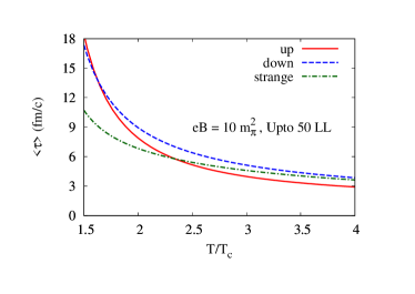
(a)

Figure 1: The temperature dependence of thermal relaxation time for quarks at $\mid eB\mid=10m_{\pi}^{2}$.

with $F(l,l^{{}^{\prime}},\xi)=[L_{l}^{(l^{{}^{\prime}}-l)}(\xi)]^{2}+\dfrac{l^{{}^{\prime}}}{l}[L_{l-1}^{(l^{{}^{\prime}}-l)}(\xi)]^{2}$ for $l>0$ and $F(l,l^{{}^{\prime}},\xi)=1$ for the lowest Landau level. Here, $\alpha_{\text{eff}}$ is the effective coupling constant and is defined from the Debye screening masses of the QGP Mitra:2017sjo ; Bandyopadhyay:2016fyd ; Ghosh:2018xhh ; Bonati:2017uvz ; Singh:2017nfa .

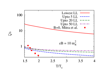
(a)

Figure 2: The effects of HLLs on the temperature behaviour of $\zeta/s$ at $\mid eB\mid=10m_{\pi}^{2}$. Behaviour of $\zeta/s$ is comparing with the result at ${\bf{B}}=0$ of Mitra et al. Mitra:2018akk .

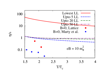
(a)

Figure 3: The effects of HLLs on the temperature behaviour of $\eta/s$ at $\mid eB\mid=10m_{\pi}^{2}$. Lattice data Nakamura:2004sy and result of Marty et al. Marty:2013ita for $\eta/s$ are in the absence of magnetic field.

Hot medium effects are entering through the quasiparton distribution function and the effective coupling. The effective thermal relaxation time controls the behaviour of transport coefficients critically. Note that in the limit $T^{2}\ll\mid q_{f}eB\mid$, LLL approximation is valid so that $X(l=0,l^{{}^{\prime}}=0,\xi)\approx 16\pi{(\alpha_{\text{eff}})}m_{f}^{2}N_{c}C_{F}$, where $e^{-\xi}\approx 1$ in this regime. Hence, the thermal relaxation time as defined in the Eq. (III) can be reduced to the LLL result as defined in Eq. (42) in the limit $T^{2}\ll\mid q_{f}eB\mid$. Following the parton distribution function within the EQPM framework, the thermal average of $\tau_{\text{eff}}$ can be defined as,

$$<\tau_{\text{eff}}>=\dfrac{\sum_{l=0}^{\infty}\int_{-\infty}^{\infty}{dp_{z}\tau_{\text{eff}}f^{0}_{q}}}{\sum_{l=0}^{\infty}\int_{-\infty}^{\infty}{dp_{z}f^{0}_{q}}}.$$ (46)

Notably, the thermal average is taken merely to explore the temperature behaviour of $<\tau_{\text{eff}}>$ with the inclusion of the effects of HLLs and analysed in the next section. While computing the transport coefficients the momentum dependence of the relaxation time, $\tau_{eff}$ has been employed.

IV Results and discussions

Let us initiate the discussion with the temperature behaviour of thermal relaxation time $\tau_{\text{eff}}$ of the quarks (up, down and strange quarks with masses $m_{u}=3$ MeV, $m_{d}=5$ MeV and $m_{s}=100$ MeV respectively) for the dominant $1\rightarrow 2$ processes in the presence of the strong magnetic field. Thermal relaxation time has been plotted as a function of $\frac{T}{T_{c}}$ for $\mid eB\mid=10m^{2}_{\pi}$ considering up to 50 LLs in the Fig. 1. The relaxation time exhibits the decreasing trend with increasing temperature. In the limit, $T^{2}\ll\mid q_{f}eB\mid$, $\tau_{\text{eff}}$ defined in Eq. (III) reduced to the LLL result as described in Kurian:2018dbn . To encode the EoS effects in the thermal relaxation, the quasiparticle parton distribution functions are introduced along with the effective coupling constant. The thermal relaxation time act as the dynamical input for the transport processes.

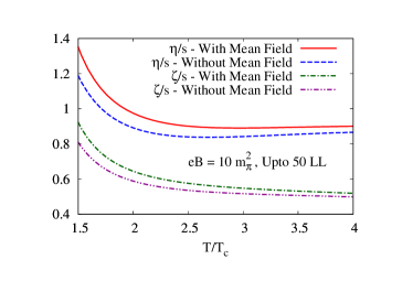
(a)

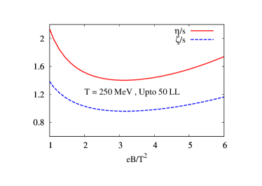
(b)

Figure 4: Temperature dependence of $\zeta/s$ and $\eta/s$ with and without mean field correction at $\mid eB\mid=10m_{\pi}^{2}$ for 1$\rightarrow$ 2 processes (left panel). Magnetic field dependence of $\zeta/s$ and $\eta/s$ (right panel).

Following the Eq. (II.0.1), the temperature dependence of bulk viscosity depends on the term $\frac{1}{\omega_{p}^{2}}(p_{z_{k}}^{2}-\omega_{p}^{2}c_{s}^{2})^{2}$ and the relaxation time $\tau_{\text{eff}}$, where $c_{s}^{2}$ can be obtained from the QCD thermodynamics. The ratio of longitudinal bulk viscosity to entropy density for the $1\rightarrow 2$ processes at $\mid eB\mid=10m^{2}_{\pi}$ has been plotted as a function of $T/T_{c}$ in the Fig. 2. The temperature dependence of the $\zeta/s$ in the strong magnetic field indicates its rising behaviour near $T_{c}$. The behaviour of longitudinal shear viscosity for the 1$\rightarrow$ 2 processes with $T/T_{c}$ at $\mid eB\mid=10m^{2}_{\pi}$ is shown in Fig. 3. Since the driving force for the longitudinal shear viscosity is in the direction of the magnetic field, the Lorentz force does not interfere in the calculation. Quantitatively, $\eta/s$ with the HLL contributions remains within the same range of the lattice data Nakamura:2004sy and NJL model result in Marty:2013ita at ${B}={0}$. This observation is in line with the result that longitudinal conductivity with HLLs contributions remains within the range of the lattice result at zero magnetic field Fukushima:2017lvb . For the numerical estimation of $\zeta/s$ and $\eta/s$, we truncate the Landau level sum at $l_{\text{max}}=50$. We observe that the HLL contributions are significant in the estimation of the viscous coefficients whereas the LLL approximation has an enhancement as $m_{f}$ tends to zero. Our observations on the effects of HLLs to the transport coefficients are qualitatively consistent with the results of the recent work of Fukushima and Hidaka Fukushima:2017lvb .

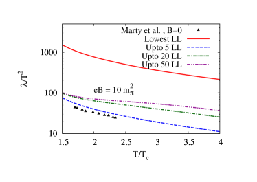
(a)

Figure 5: Thermal conductivity as a function of $T/T_{c}$ at $\mid eB\mid=10m_{\pi}^{2}$. Behaviour of $\lambda/T^{2}$ is comparing with the result at ${\bf{B}}=0$ of Marty et al. Marty:2013ita

The present analysis is done by employing the effective covariant kinetic theory using the Chapman-Enskog method including the effects of HLLs. The mean field force term which emerges from the effective theory indeed appears as the mean field corrections to the transport coefficients. The second term in the Eq. (II.0.1) and Eq. (II.0.1) describes the mean field contribution to the longitudinal shear viscosity and bulk viscosity in the strong magnetic field, respectively. The mean field term consists of the term $\delta\omega$ which is the temperature gradient of the effective fugacity $z_{g/q}$. The temperature behaviours of the viscous coefficients (bulk and shear viscosities) in the presence of strong magnetic field with and without the mean field corrections are shown in Fig. 4 (left panel). At higher temperature, the effects are negligible since the effective fugacity behaves as a slowly varying function of temperature there. Hence, the mean field corrections due to the quasiparticle excitations are significant at temperature region closer to $T_{c}$. The magnetic field dependence of the bulk viscosity and shear viscosity have been plotted in the Fig. 4(right panel). In the strong magnetic field limit, the viscous coefficients could be computed within LLL approximation. The inclusion of HLLs reflects the non-trivial (non-monotonic) magnetic field dependence of the transport coefficients. Similar non-monotonic structure in the magnetic field dependence of longitudinal conductivity with HLLs is described in Fukushima:2017lvb . The estimation of electric conductivity within our model while including the HLLs is beyond the scope of the present analysis and is a matter of future investigations.

Mean field corrections to the thermal conductivity is explicitly shown in Eq. (II.0.2) in which thermal relaxation incorporates the microscopic interactions. We depicted the temperature behaviour of $\lambda/T^{2}$ in Fig. 5. The HLL effects of the transport coefficients are entering through the thermal relaxation time and the quasiparticle distribution function. These effects are significant in the estimation of transport coefficients in the presence of a magnetic field. The temperature behaviour of the dimensionless quantity $\lambda/T^{2}$ in the absence of the magnetic field is well investigated Mitra:2017sjo ; Marty:2013ita and is in the order of $100-25$ within the temperature range $(1-4)\frac{T}{T_{c}}$, which is quantitatively consistent with our result.

V Conclusion and Outlook

In conclusion, we have computed the temperature behaviour of the transport parameters such as longitudinal viscous coefficients (shear and bulk viscosities) and thermal conductivity for the $1\rightarrow 2$ processes in the strong magnetic field background while including the effects of HLLs. Thermal relaxation time is computed in the strong magnetic field incorporating the HLL contributions. Setting up an effective covariant kinetic theory within EQPM in the strong magnetic field induces mean field contributions to the transport coefficients. We employed the Chapman-Enskog method in the effective kinetic theory for the computation of transport coefficients. The transport coefficients that have been estimated are influenced by the thermal medium and magnetic field. Hot QCD effects are incorporated through the quasiparton degrees of freedom along with effective coupling and the medium effects are found to be negligible at very high temperature. We focused on the weakly coupled regime of the perturbative QCD within the limit $gT\ll\sqrt{\mid q_{f}eB\mid}$ in which higher Landau level (HLL) contributions are significant. Notably, the inclusion of HLL contributions are essential to explain the transport processes at high temperature in the presence of the magnetic field. Furthermore, effects of the mean field term are seen to be quite significant as fas as the temperature behavior of the above mentioned transport coefficients is concerned (for the temperatures which are not very far away from $T_{c}$).

An immediate future extension of the work is to investigate the aspects of non-linear electromagnetic responses of the hot QGP with the mean field contribution along with the effective description of magnetohydrodynamic waves in the hot QGP medium. In addition, the estimation of all transport coefficients from covariant kinetic theory within the effective fugacity quasiparticle model using more realistic collision integral, for example, BGK (Bhatnagar, Gross and Krook) collision term, in the strong magnetic field would be another direction to work.

References

- (1) Adams et al. (STAR Collaboration), Nucl. Phys. A757, 102 (2005); K. Adcox et al. (PHENIX Collaboration), Nucl. Phys. A757, 184 (2005); B.B. Back et al. (PHOBOS Collaboration), Nucl. Phys. A757, 28 (2005); A. Arsence et al. (BRAHMS Collaboration), Nucl. Phys. A757, 1 (2005).
- (2) K. Aamodt et al. [ALICE Collaboration], Phys. Rev. Lett. 105, 252301 (2010).
- (3) V. Skokov, A. Y. Illarionov and V. Toneev, Int. J. Mod. Phys. A 24, 5925 (2009).
- (4) Y. Zhong, C. B. Yang, X. Cai and S. Q. Feng, Adv. High Energy Phys. 2014 (2014) 193039.
- (5) W.-T. Deng, and Xu-Guang Huang, Phys. C 85, 044907 (2012).
- (6) S. K. Das, S. Plumari, S. Chatterjee, J. Alam, F. Scardina and V. Greco, Phys. Lett. B 768, 260 (2017).
- (7) G. Inghirami, L. Del Zanna, A. Beraudo, M. H. Moghaddam, F. Becattini and M. Bleicher, Eur. Phys. J. C 76, no. 12, 659 (2016).
- (8) L. Del Zanna et al., Eur. Phys. J. C 73, 2524 (2013).
- (9) F. Becattini et al., Eur. Phys. J. C 75, no. 9, 406 (2015).
- (10) K. Fukushima, D. E. Kharzeev and H. J. Warringa, Phys. Rev. D 78, 074033 (2008), D. E. Kharzeev, L. D. McLerran, H. J. Warringa, Nucl. Phys. A803, 227 (2008),D. E. Kharzeev, Annals Phys. 325, 205 (2010), D. E. Kharzeev and D. T. Son, Phys. Rev. Lett. 106, 062301 (2011).
- (11) A. V. Sadofyev and M. V. Isachenkov, Phys. Lett. B 697, 404 (2011), A. V. Sadofyev, V. I. Shevchenko and V. I. Zakharov, Phys. Rev. D 83, 105025 (2011).
- (12) X. G. Huang, Y. Yin, and J. Liao Nucl. Phys. A956, 661 (2016).
- (13) D. E. Kharzeev, J. Liao, S. A. Voloshin and G. Wang, Prog. Part. Nucl. Phys. 88, 1 (2016).
- (14) A. Avkhadiev and A. V. Sadofyev, Phys. Rev. D 96, no. 4, 045015 (2017).
- (15) N. Yamamoto, Phys. Rev. D 96, no. 5, 051902 (2017).
- (16) L. Adamczyk et al. [STAR Collaboration], Nature 548, 62 (2017).
- (17) F. Becattini, I. Karpenko, M. Lisa, I. Upsal and S. Voloshin, Phys. Rev. C 95, no. 5, 054902 (2017).
- (18) M. Luzum and P. Romatschke, Phys. Rev. C 78, 034915 (2008) Erratum: [Phys. Rev. C 79, 039903 (2009)].
- (19) J. Adam et al. [ALICE Collaboration], Phys. Rev. Lett. 117, 182301 (2016), J. Adam et al. [ALICE Collaboration], Phys. Rev. Lett. 116, no. 13, 132302 (2016).
- (20) B. Abelev et al. [ALICE Collaboration], Phys. Rev. Lett. 111, no. 23, 232302 (2013).
- (21) J. Adam et al. [ALICE Collaboration], JHEP 1609, 164 (2016).
- (22) K. Hattori, X. G. Huang, D. H. Rischke and D. Satow, Phys. Rev. D 96, no. 9, 094009 (2017).
- (23) M. Kurian and V. Chandra, Phys. Rev. D 96, no. 11, 114026 (2017).
- (24) D. Kharzeev and K. Tuchin, JHEP 0809, 093 (2008).
- (25) G. D. Moore and O. Saremi, JHEP 0809, 015 (2008).
- (26) A. Czajka and S. Jeon, Phys. Rev. C 95, no. 6, 064906 (2017).
- (27) A. Nakamura and S. Sakai, Phys. Rev. Lett. 94, 072305 (2005).
- (28) N. Astrakhantsev, V. Braguta and A. Kotov, JHEP 1704, 101 (2017).
- (29) N. Y. Astrakhantsev, V. V. Braguta and A. Y. Kotov, arXiv:1804.02382 [hep-lat].
- (30) K. Tuchin, J. Phys. G 39, 025010 (2012).
- (31) R. Marty, E. Bratkovskaya, W. Cassing, J. Aichelin and H. Berrehrah, Phys. Rev. C 88, 045204 (2013).
- (32) S. Mitra and V. Chandra, Phys. Rev. D 96, no. 9, 094003 (2017).
- (33) K. Fukushima and Y. Hidaka, Phys. Rev. Lett. 120, no. 16, 162301 (2018).
- (34) K. Hattori, S. Li, D. Satow and H. U. Yee, Phys. Rev. D 95, no. 7, 076008 (2017).
- (35) P. B. Arnold, G. D. Moore and L. G. Yaffe, JHEP 0305, 051 (2003).
- (36) M. A. Valle Basagoiti, Phys. Rev. D 66, 045005 (2002).
- (37) G. D. Moore, JHEP 0105, 039 (2001).
- (38) J. W. Chen, H. Dong, K. Ohnishi and Q. Wang, Phys. Lett. B 685, 277 (2010).
- (39) A. S. Khvorostukhin, V. D. Toneev and D. N. Voskresensky, Phys. Rev. C 83, 035204 (2011).
- (40) Z. Xu and C. Greiner, Phys. Rev. Lett. 100, 172301 (2008).
- (41) L. Thakur, P. K. Srivastava, G. P. Kadam, M. George and H. Mishra, Phys. Rev. D 95, no. 9, 096009 (2017).
- (42) V. Chandra and V. Ravishankar, Phys. Rev. D 84, 074013 (2011).
- (43) V. Chandra, R. Kumar and V. Ravishankar, Phys. Rev. C 76, 054909 (2007).
- (44) S. Mitra and V. Chandra, Phys. Rev. D 94, no. 3, 034025 (2016).
- (45) S. Mitra and V. Chandra, Phys. Rev. D 97, no. 3, 034032 (2018).
- (46) M. Kurian and V. Chandra, Phys. Rev. D 97, no. 11, 116008 (2018).
- (47) K. Fukushima, K. Hattori, H. U. Yee and Y. Yin, Phys. Rev. D 93, no. 7, 074028 (2016)
- (48) V. M. Bannur, Phys. Rev. C 75, 044905 (2007); Phys. Lett. B 647, 271 (2007); JHEP 0709, 046 (2007).
- (49) A. Dumitru, R. D. Pisarski, Phys. Lett. B 525, 95 (2002); K. Fukushima, Phys. Lett. B 591, 277 (2004); S. K. Ghosh et. al, Phys. Rev. D 73, 114007 (2006); H. Abuki, K. Fukushima, Phys. Lett. B 676, 57 (2006); H. M. Tsai, B. Muller, J. Phys. G 36, 075101 (2009).
- (50) M. D’Elia, A. Di Giacomo and E. Meggiolaro, Phys. Lett. B 408, 315 (1997); Phys. Rev. D 67, 114504 (2003); P. Castorina, M. Mannarelli, Phys. Rev. C 75, 054901 (2007); Phys. Lett. B 664, 336 (2007).
- (51) N. Su and K. Tywoniuk, Phys. Rev. Lett. 114, no. 16, 161601 (2015).
- (52) W. Florkowski, R. Ryblewski, N. Su, and K. Tywoniuk, Phys. Rev. C 94, 044904 (2016); Acta Phys. Pol. B 47, 1833 (2016).
- (53) A. Bandyopadhyay, N. Haque, M. G. Mustafa and M. Strickland, Phys. Rev. D 93, no. 6, 065004 (2016).
- (54) M. Cheng et al., Phys. Rev. D 77, 014511 (2008).
- (55) S. Borsanyi, Z. Fodor, C. Hoelbling, S. D. Katz, S. Krieg, Kalman K. Szabo, Phys. Lett. B 370, 99-104 (2014).
- (56) N. Haque, A. Bandyopadhyay, J. O. Andersen, Munshi G. Mustafa, M. Strickland and Nan Su, JHEP 1405, 027 (2014).
- (57) J. O. Andersen, N. Haque, M. G. Mustafa and M. Strickland, Phys. Rev. D 93, 054045 (2016).
- (58) F. Bruckmann, G. Endrodi, M. Giordano, S. D. Katz, T. G. Kovacs, F. Pittler and J. Wellnhofer, Phys. Rev. D 96, no. 7, 074506 (2017).
- (59) A. N. Tawfik, J. Phys. Conf. Ser. 668, no. 1, 012082 (2016).
- (60) V. P. Gusynin, V. A. Miransky and I. A. Shovkovy, Nucl. Phys. B 462, 249 (1996).
- (61) S. Li and H. U. Yee, Phys. Rev. D 97, no. 5, 056024 (2018).
- (62) K. Tuchin, Adv. High Energy Phys. 2013, 490495 (2013).
- (63) D. D. Ofengeim and D. G. Yakovlev, EPL 112, no. 5, 59001 (2015).
- (64) K. Hattori and D. Satow, Phys. Rev. D 94, no. 11, 114032 (2016).
- (65) A. Bandyopadhyay, C. A. Islam and M. G. Mustafa, Phys. Rev. D 94, no. 11, 114034 (2016).
- (66) S. Ghosh and V. Chandra, arXiv:1808.05176 [hep-ph].
- (67) C. Bonati, M. D’Elia, M. Mariti, M. Mesiti, F. Negro, A. Rucci and F. Sanfilippo, Phys. Rev. D 95, no. 7, 074515 (2017).
- (68) B. Singh, L. Thakur and H. Mishra, Phys. Rev. D 97, no. 9, 096011 (2018).