Enhanced Pricing and Management of Bundled Insurance Risks with Dependence-aware Prediction using Pair Copula Construction

Abstract

We propose a dependence-aware predictive modeling framework for multivariate risks stemmed from an insurance contract with bundling features – an important type of policy increasingly offered by major insurance companies. The bundling feature naturally leads to longitudinal measurements of multiple insurance risks, and correct pricing and management of such risks is of fundamental interest to financial stability of the macroeconomy. We build a novel predictive model that fully captures the dependence among the multivariate repeated risk measurements. Specifically, the longitudinal measurement of each individual risk is first modeled using pair copula construction with a D-vine structure, and the multiple D-vines are then integrated by a flexible copula. While our analysis mainly focuses on multivariate insurance risks, the proposed model indeed contributes to the broad research area of longitudinal data analysis. In particular, it provides a unified modeling framework for multivariate longitudinal data that can accommodate different scales of measurements, including continuous, discrete, and mixed observations, and thus can be potentially useful for various economic studies. A computationally efficient sequential method is proposed for model estimation and inference, and its performance is investigated both theoretically and via simulation studies. In the application, we examine multivariate bundled risks in multi-peril property insurance using proprietary data from a commercial property insurance provider. The proposed model is found to provide improved decision making for several key insurance operations. For underwriting, we show that the experience rate priced by the proposed model leads to a 9% lift in the insurer’s net revenue. For reinsurance, we show that the insurer underestimates the risk of the retained insurance portfolio by 10% when ignoring the dependence among bundled insurance risks.

Keywords: Multivariate longitudinal data, Copula, D-Vine, Insurance operations, Predictive analytics, Graphical model

1 Introduction

In the past decade, insurance industry, especially property and casualty insurance, has been advancing the use of predictive analytics to leverage big data and improve business performance. Statistical learning of insurance risks has become an essential component in the data-driven decision making in various insurance operations (Frees,, 2015). This study focuses on the predictive modeling for nonlife insurance products with a bundling feature.

Bundling is an increasingly popular design in modern short-term insurance contracts and can take different forms in practice: a comprehensive auto insurance policy provides coverage for both collision and third-party liability; employee compensation insurance provides benefits for wage replacement, medical treatment, and vocational rehabilitation; an open peril property insurance policy covers losses due to all types of causes subject to certain exclusions. As another prominent example, in personal lines of business, auto insurance and homeowner insurance are often marketed to households as a package. The bundling feature naturally leads to longitudinal measurements of multivariate risks, where the insurer observes multiple risk outcomes of an insurance contract over time. This serves as motivation of our study and we aim to propose a general framework of predictive modeling for multivariate insurance risks with longitudinal/repeated measurements.

An essential element of predictive modeling is to accurately assess the dependence/association among insurance risks, which helps track the evolution and thus generate prediction of future risks. Two types of dependence are of primary interests to insurers and have been studied in separate strands of literature. The first is the temporal dependence of a single insurance risk. The availability of longitudinal measurements allows an insurer to adjust a policyholder’s premium based on the claim history, known as experience rating in insurance (Pinquet,, 2013). The experience rate is determined by the insurer’s ability of learning hidden risks of policyholders that evolve over time (see e.g. Frees and Wang, (2006), Boucher and Inoussa, (2014) and Oh et al., (2020)). The second is the contemporaneous dependence among multiple insurance risks. Correlated claims induces concentration risk in the insurance portfolio on the liability side of an insurer’s book, thus understanding the effects of dependence in risk aggregation can provide valuable guidance to the insurer’s operation in claim management (Frees and Valdez, (2008) and Jessup et al., (2020)) and capital management (Bernard et al., (2014) and Wang et al., (2019)).

The multivariate longitudinal measurements of insurance risks from bundling contracts naturally involve both temporal and contemporaneous dependence. Thus, a predictive model that allows a joint analysis of the two types of dependence can deliver unique insights to an insurer’s operation and enable an insurer to perform prospective experience rating, determine optimal risk retention, and estimate the amount of risk capital in a coherent and consistent manner. However, despite the appealing benefits, the majority of existing models in the literature are only capable of examining the two types of dependence separately. The scarcity of a unified and flexible predictive modeling framework for multivariate insurance risks is due to several challenges.

A notable challenge is the discreteness in the risk measurements. A common measurement of a policyholder’s risk is the annual number of claims incurred (Denuit et al.,, 2007). Thus, in the context of bundling insurance products, we need to jointly model multivariate claim counts stemmed from each of the multiple insurance risks covered in the contract. Due to the discreteness of claim count, the classical concept of correlation and existing modeling and analysis techniques for multivariate continuous data are not applicable (Joe,, 2014). Another challenge in predictive modeling is to determine the optimal number of historical observations to be used in the prediction for future risks. Existing literature mostly models temporal dependence among insurance outcomes by borrowing techniques (notably the autoregressive models) from the time series forecasting literature. However, predictive models and specification tests of optimal order for time series data (which consists of hundreds of observations along time dimension) are generally not appropriate for longitudinal data (which only contains a handful of temporal observations).

We remark that several strategies have been studied for modeling multivariate longitudinal data in the biostatistics literature, see Verbeke et al., (2014) and Farewell et al., (2017) for recent reviews. However, these methods are typically built upon random effect or latent variable models, which offer limited modeling choices for marginal behavior and only allows for specific structures on the temporal-contemporaneous dependence. Moreover, these methods typically are designed for continuous data and become computationally infeasible for insurance claim counts, and discrete data in general, especially in the setting of nonstandard marginal distributions. To conserve space, we refer to Section LABEL:subsec:add_litreview of the supplementary material for more detailed review of this literature.

To fill the gap in the literature, we propose a unified predictive modeling framework for multivariate longitudinal measurements of insurance risks that simultaneously accommodates the temporal and contemporaneous dependence. Specifically, we integrate a generalized linear regression based framework with a flexible graphical model named vine (Bedford and Cooke,, 2002; Aas et al.,, 2009), where the longitudinal measurement of each individual risk is first modeled using pair copula construction with a D-vine structure, and the multiple D-vines are then linked together via a flexible multivariate copula. We refer to Section 3 for the technical definition and more detailed literature review of copula and vine.

We remark that as a fundamental tool for modeling dependence, copula has been widely studied in the econometrics literature, see Chen and Fan, 2006a ; Chen and Fan, 2006b ; Chen et al., (2009); Beare, (2010); Oh and Patton, (2013, 2017); Chen et al., (2021) for representative works. However, all these works primarily focus on multivariate time series modeling (with continuous observations) and cannot be easily adapted to model multivariate longitudinal data. Indeed, to our best knowledge, copula-based models for multivariate longitudinal data are still scarce in the literature.

Our work provides one of the first effort in constructing copula-based models for multivariate longitudinal data. Due to the use of copula, the proposed framework allows for separate specification of the marginal regression model from the dependence model, and thus enables unified accommodation for different scales of multivariate longitudinal data, including continuous, discrete, and mixed outcomes. Moreover, the D-vine based pair copula construction is flexible and further allows the proposed model to specify the temporal and contemporaneous dependence unrestrictedly, and thus can achieve a wide range and various types of dependence among multivariate longitudinal measurements. Thanks to these important properties, the proposed model can be useful for modeling multivariate longitudinal data commonly encountered under various economic studies and thus contributes to the broad research area of longitudinal data analysis. We further develop diagnostic checks for model specification and propose a novel data-driven procedure that automatically determines the optimal weight given to historical observations for future risk prediction. We propose a computationally efficient sequential method for the estimation and inference of the proposed model and investigate its performance both theoretically and via simulation studies.

Compared to standard modeling practice in the insurance industry, the proposed predictive model achieves simultaneous modeling of both temporal and contemporaneous dependence among bundled insurance risks and provides dependence-aware prediction that is shown to bring significant values to key insurance operations such as risk segmentation and risk management. Specifically, using data from a Wisconsin property insurance provider, we show that the risk pricing derived from the proposed predictive model provides a 9% lift of the insurer’s profit in the underwriting and ratemaking operation, and the proposed model provides more truthful risk assessment of the retained insurance portfolio of the insurer by 10% in the reinsurance operation.

The rest of the paper is structured as follows. Section 2 highlights the essential role of predictive models in improving decision making for insurance operations. Section 3 introduces the pair copula construction based unified modeling framework for multivariate longitudinal data. Section 4 proposes a sequential inference procedure for model selection and estimation, and further establishes its theoretical guarantees and performs simulation studies. Section 5 conducts empirical analysis of multivariate claim counts from a large-scale Wisconsin property insurance program. Section 6 illustrates managerial implications and significance of the proposed dependence-aware predictive model in key insurance operations. Section 7 concludes. Technical materials, additional simulation experiments and data analysis results are gathered in the supplementary material.

2 Predictive Modeling in Key Insurance Operations

In this section, we discuss the use of predictive modeling in insurance operations and the decision-makings faced by insurers for managing a portfolio of insurance contracts with bundled risks.

Denote $y_{it}^{(j)}$ as the measurement (such as annual claim count) of the $j$th ($=1,\cdots,J$) insurance risk for policyholder $i$ ($=1,\ldots,n$) in period $t$ ($=1,\ldots,T$). The number of observations $T$ is typically small, partly due to the short-term nature of nonlife insurance contracts. Let $\bm{x}_{it}^{(j)}$ be the set of exogenous predictors the insurer uses for evaluating the $j$th risk of policyholder $i$ in period $t$, such as characteristics of the policyholder or the contract (see Table LABEL:tab:covariates in the supplementary material for an example). Define $\bm{x}_{i}^{(j)}=\{\bm{x}_{it}^{(j)}:t\geq 1\}$. Define $H_{it}^{(j)}=\bm{x}_{i}^{(j)}\bigcup\{y_{is}^{(j)}:s=1,\ldots,t\}$, which includes the history of the $j$th risk up to period $t$ for policyholder $i$, together with the exogenous predictors. Note that since the predictors are exogenous, without loss of generality, we can assume that we have the knowledge of $\bm{x}_{i}^{(j)}$ at all time periods $t$ for notational simplicity.

Statistically speaking, we define the predictive model for the multivariate insurance risks $\bm{y}_{i,T+1}=(y^{(1)}_{i,T+1},\ldots,y^{(J)}_{i,T+1})$ of policyholder $i$ ($=1,\cdots,n$) in the future period $T+1$ as

$$F\left(\bm{y}_{i,T+1}|H_{iT}^{(1)},\ldots,H_{iT}^{(J)}\right)=F\left(y^{(1)}_{i,T+1},\ldots,y^{(J)}_{i,T+1}|H_{iT}^{(1)},\ldots,H_{iT}^{(J)}\right),$$ (1)

which is the conditional joint distribution of future multivariate insurance risks $\bm{y}_{i,T+1}$ given its claim history and exogenous predictors. Importantly, the conditional distribution (1) involves both temporal and contemporaneous dependence among $\{\bm{y}_{i,1},\bm{y}_{i,2},\cdots,\bm{y}_{i,T+1}\}$. We show below that an accurate modeling of (1) is essential for informed decision making in key insurance operations.

Assuming the measurement of risk $y_{it}^{(j)}$ represents the claim count, we can express the aggregate losses of the bundled insurance contract stemmed from policyholder $i$ in period $T+1$ as:

$$S_{i,T+1}=\alpha_{i,T+1}^{(1)}y_{i,T+1}^{(1)}+\cdots+\alpha_{i,T+1}^{(J)}y_{i,T+1}^{(J)},$$ (2)

where $\alpha_{i,T+1}^{(j)}$ represents the average cost per claim for the $j$th risk of policyholder $i$. In this study, our primary focus is the dependence among claim frequency, we thus assume one has prior knowledge on the average claim cost (de Jong and Heller,, 2008).

The first insurance operation of interest is regarding risk segmentation, specifically renewal underwriting and ratemaking. Since nonlife insurance contracts in general have short duration, the insurer has the opportunity to decide whether to provide coverage (underwriting) when the current contract expires and is subject to renewal. Provided that the insurer accepts the risk, a new premium is to be determined (ratemaking). Ratemaking at renewal is based on two types of information, the exogenous rating variables and the policyholder’s claim history. Adjusting premiums using the claim history is known as experience rating. In the actuarial statistics literature, credibility theory has long been introduced as a comprehensive way of incorporating loss experience into pricing (see Bühlmann and Gisler, (2005)). Frees et al., (1999) established the connection between the credibility theory and longitudinal data models.

Given a deductible $d\geq 0$, a risk retention feature commonly found in property and health insurance contracts, the experience rate is based on the expected loss cost in period $T+1$

$$\mathbb{E}\left((S_{i,T+1}-d)_{+}|H_{iT}^{(1)},\ldots,H_{iT}^{(J)}\right),$$ (3)

where $(S_{i,T+1}-d)_{+}=\max\{S_{i,T+1}-d,0\}$. The insurer uses the experience rate (3) to decide whether to provide coverage and to adjust the premium upon acceptance of the risk. The expected loss in (3) depends on $S_{i,T+1}$, whose behavior is effectively determined by the conditional distribution (1), manifesting the crucial value of accurate predictive modeling of temporal and contemporaneous dependence among bundled insurance risks.

The second insurance operation under consideration is reinsurance. As a risk management tool, insurers use reinsurance to reduce and stabilize the cost of insurance while taking into account its own risk transfer capacity. In particular, the insurer often cedes some of its portfolio risk to an reinsurer to reduce its liability when it is subject to underwriting capacity (Albrecher et al.,, 2017). We examine the quota share treaty, a form of pro-rata reinsurance popular in the insurance industry, in which the reinsurer assumes an agreed percentage of each insurance risk in the portfolio and shares all premiums and losses accordingly with the insurer.

For an insurer’s portfolio of $n$ bundled insurance contracts $\{S_{i,T+1}:i=1,\ldots,n\}$, we consider the general case of quota share treaty where the retention can vary by contract. Let $\delta_{i}$ denote the retained quota for the $i$th contract, the retained risk of the insurer can be represented by

$$S_{T+1}^{*}=\delta_{1}S_{1,T+1}+\cdots+\delta_{n}S_{n,T+1},$$ (4)

where $S_{i,T+1}$ is defined in (2). The insurer’s goal is to find optimal amount of retention $\{\delta_{1},\cdots,\delta_{n}\}$ across the $n$ contracts to minimize volatility of the retained risk $S_{T+1}^{*}$ under constraints on its underwriting capacity $\mathbb{E}(S_{T+1}^{*})$. It is evident that both temporal and contemporaneous dependence among the multivariate insurance risks in (1) directly impact the behavior of $S_{i,T+1}$ and thus are critical to the calculation of optimal risk retention $\delta_{i}$ in the portfolio risk management.

3 Methodology

To model longitudinal measurements of multivariate insurance risks, we propose an approach that integrates a regression-based framework with a flexible graphical model named vine (Bedford and Cooke,, 2001, 2002), also known as pair copula construction (Aas et al.,, 2009) in the literature.

The vine model can be seen as a special type of copula. A $d$-dimensional copula is a multivariate distribution function on $(0,1)^{d}$ with uniform margins. By the celebrated Sklar, (1959)’s theorem, any multivariate distribution $F$ can be separated into its marginals $(F_{1},\ldots,F_{d})$ and a copula $C$, where the copula captures all the scale-free dependence of the multivariate distribution. In particular, denote $\mathbf{Z}\in\mathbb{R}^{d}$ as a random vector following a multivariate distribution $F$, we have $F(z_{1},\ldots,z_{d})=C(F_{1}(z_{1}),\ldots,F_{d}(z_{d}))$ for any $(z_{1},\ldots,z_{d})\in\mathbb{R}^{d}$.

The key feature of vine is that it provides a systematic framework of building flexible multivariate distributions based on a sequence of bivariate copulas. The original literature of vine mainly focused on modeling multivariate data with continuous outcomes, see Kurowicka and Cooke, (2006) and Aas et al., (2009) for early works. Vine has received extensive attention in the recent literature of dependence modeling, due to its flexibility especially in terms of modeling tail dependence and asymmetric dependence (see e.g. Joe and Kurowicka, (2011)). Building upon the framework for continuous outcomes, Panagiotelis et al., (2012) introduced pair copula construction for discrete data, Stöber et al., (2015) examined the vine model for multivariate responses with both continuous and discrete variables, Shi and Yang, (2018) employed pair copula construction to model temporal dependence among univariate longitudinal data with mixed outcomes, and Barthel et al., (2018) further extended the vine approach to event time data with censoring. However, all these studies focus on univariate longitudinal data or multivariate observations without repetition, pair copula construction for multivariate longitudinal data with multilevel structure is sparse in the literature. Recently, Brechmann and Czado, (2015) and Smith, (2015) discussed possible strategies of constructing vines for multivariate time series. However, the models therein only accommodates continuous observations and cannot be easily adapted to model multivariate longitudinal data.

Based on pair copula construction, we propose a unified modeling framework for multivariate longitudinal data in Section 3.1 and further present its detailed application for modeling and predicting longitudinal observations of multivariate insurance claim counts in Sections 3.2 and 3.3.

3.1 A Unified Modeling Framework

In this section, we present a unified modeling framework for multivariate longitudinal data that can accommodate different scales of measurements, including continuous, discrete, and mixed outcomes.

Following notations in Section 2, for policyholder $i=1,\cdots,n$, we denote $\bm{H}_{it}=(H_{it}^{(1)},\ldots,H_{it}^{(J)})$ as its claim history up to time $t$, denote $\bm{X}_{i}=\{\bm{x}_{i}^{(1)},\cdots,\bm{x}_{i}^{(J)}\}$ as the collection of its exogenous predictors, and further define $\bm{H}_{i0}=\bm{X}_{i}.$ In the following, we use $f$ to denote the (conditional) pmf or pdf for either univariate or multivariate distributions, and use $F$ to denote the corresponding cdf. Denote $\bm{y}_{it}=(y_{it}^{(1)},\cdots,y_{it}^{(J)})$. Given the exogenous predictors $\bm{X}_{i}$, the joint distribution of the observed multivariate insurance risks $\{\bm{y}_{i1},\ldots,\bm{y}_{iT}\}$ for policyholder $i$ can be written as

$$f(\bm{y}_{i1},\ldots,\bm{y}_{iT}|\bm{X}_{i})=f(\bm{y}_{i1}|\bm{X}_{i})f(\bm{y}_{i2}|\bm{y}_{i1};\bm{X}_{i})\cdots f(\bm{y}_{iT}|\bm{y}_{i1},\ldots,\bm{y}_{iT-1};\bm{X}_{i})=\prod_{t=1}^{T}f(\bm{y}_{it}|\bm{H}_{i,t-1}).$$ (5)

Note that the conditional decomposition in (5) is generic and does not impose any constraint on the model specification of $(\bm{y}_{i1},\ldots,\bm{y}_{iT})|\bm{X}_{i}$. In other words, the decomposition (5) applies to all scales of measurements, including continuous, discrete, and mixed outcomes.

By the Sklar, (1959)’s theorem and its extension (Patton,, 2006), there exists a $J$-variate copula $C^{J}$ such that the corresponding cdf of the joint distribution of $\bm{y}_{it}=(y_{it}^{(1)},\ldots,y_{it}^{(J)})$ conditioning on $\bm{H}_{i,t-1}$ in (5) can be further represented as

$$F(\bm{y}_{it}|\bm{H}_{i,t-1})=C^{J}\left(F\left(y_{it}^{(1)}|H_{i,t-1}^{(1)}\right),\ldots,F\left(y_{it}^{(J)}|H_{i,t-1}^{(J)}\right)\right),$$ (6)

for $t=1,\cdots,T$. The copula $C^{J}$ captures the contemporaneous dependence among the multivariate insurance risks $\bm{y}_{it}=(y_{it}^{(1)},\ldots,y_{it}^{(J)})$, and the conditional marginal distribution $F(y_{it}^{(j)}|H_{i,t-1}^{(j)})$ captures the temporal dependence within the $j$th individual insurance risk and characterizes the behavior of $y_{it}^{(j)}$ conditioned on its claim history and exogenous predictors, for $j=1,\cdots,J$. It is important to point out that, according to the definition in (1), we can construct a predictive model for bundled insurance risks based on (6) by setting $t=T+1$.

Note that the conditional distribution $F(y_{it}^{(j)}|H_{i,t-1}^{(j)})$ in (6) can be derived from the joint distribution of $(y_{i1}^{(j)},\ldots,y_{iT}^{(j)})\big{|}\bm{x}_{i}^{(j)}$ for $j=1,\ldots,J$. For flexibility of the predictive model, we construct this joint distribution via pair copula construction based on a D-vine structure. Figure 1 shows a graphical representation of a D-vine for $T=5$. The fully specified D-vine contains $T-1=4$ trees $T_{1},\cdots,T_{4}$. In each tree, only adjacent nodes are connected by an edge, and edges become nodes in the next tree. Each node represents a (conditional) distribution and the edge indicates a bivariate copula linking the distributions of the two connecting nodes. The edges of the entire D-vine summarize the bivariate copulas that contribute to the pair copula construction. We later provide more concrete and detailed discussion of D-vine.

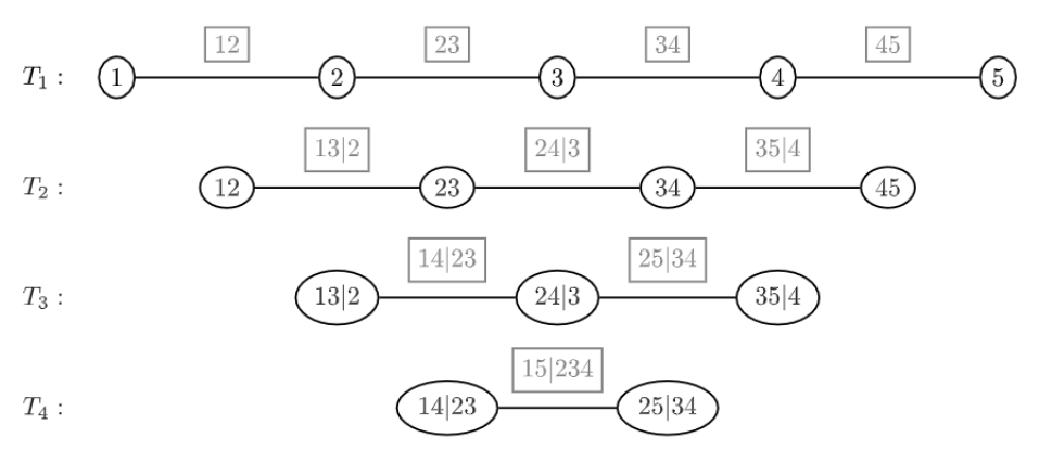
Figure 1: Graphical representation of a fully specified 5-dimensional D-vine.

Based on the graphical representation of D-vine, the joint distribution of $(y_{i1}^{(j)},\ldots,y_{iT}^{(j)})\big{|}\bm{x}_{i}^{(j)}$ can be nicely written as a factor form such that

$$f\left(y_{i1}^{(j)},\ldots,y_{iT}^{(j)}|\bm{x}_{i}^{(j)}\right)$$

$$= \prod_{t=1}^{T}f\left(y_{it}^{(j)}|\bm{x}_{i}^{(j)}\right)\prod_{t=2}^{T}\prod_{s=1}^{t-1}\frac{f\left(y^{(j)}_{is},y^{(j)}_{it}|y^{(j)}_{is+1},\ldots,y^{(j)}_{it-1};\bm{x}_{i}^{(j)}\right)}{f\left(y^{(j)}_{is}|y^{(j)}_{is+1},\ldots,y^{(j)}_{it-1};\bm{x}_{i}^{(j)}\right)f\left(y^{(j)}_{it}|y^{(j)}_{is+1},\ldots,y^{(j)}_{it-1};\bm{x}_{i}^{(j)}\right)}.$$ (7)

Here and after, for two indices $e_{1},e_{2}\in\{1,2,\cdots,T\}$, we use the convention that $(y^{(j)}_{ie_{1}},\ldots,y^{(j)}_{ie_{2}})=\varnothing$ if $e_{2}>e_{1}.$ We remark that, same as (5), the decomposition in (3.1) is generic and does not impose any constraint on the joint distribution of $(y_{i1}^{(j)},\ldots,y_{iT}^{(j)})\big{|}\bm{x}_{i}^{(j)}$, and thus accommodates all scales of measurements, including continuous, discrete, and mixed outcomes.

For more intuition, we map the decomposition in (3.1) to Figure 1. Specifically, the nodes in tree 1 (i.e. $T_{1}$) represent the univariate marginal distribution $f(y_{it}^{(j)}|\bm{x}_{i}^{(j)})$ of $y_{it}^{(j)}$ observed at each time $t=1,\cdots,T$. For $t=2,\cdots,T$ and $s=1,\cdots,t-1$, from left to right, the $s$th edge in tree $t-s$ (i.e. $T_{t-s}$) of Figure 1 corresponds to a bivariate copula, denoted by $C^{(j)}_{s,t}$. The bivariate copula $C^{(j)}_{s,t}$ is used to specify the conditional joint distribution $f(y^{(j)}_{is},y^{(j)}_{it}|y^{(j)}_{is+1},\ldots,y^{(j)}_{it-1};\bm{x}_{i}^{(j)})$ in (3.1) by linking the $s$th and $(s+1)$th nodes in tree $t-s$, which record the conditional distributions $f(y^{(j)}_{is}|y^{(j)}_{is+1},\ldots,y^{(j)}_{it-1};\bm{x}_{i}^{(j)})$ and $f(y^{(j)}_{it}|y^{(j)}_{is+1},\ldots,y^{(j)}_{it-1};\bm{x}_{i}^{(j)})$ respectively. In other words, the $s$th edge in tree $t-s$ of the D-vine represents a bivariate copula $C^{(j)}_{s,t}$, which characterizes the joint behavior of $y^{(j)}_{is}$ and $y^{(j)}_{it}$ conditional on observations $y^{(j)}_{is+1},\ldots,y^{(j)}_{it-1}$ in between.

Thanks to the use of D-vine, the decomposition in (3.1) separates the specification of the joint distribution $f(y_{i1}^{(j)},\ldots,y_{iT}^{(j)}|\bm{x}_{i}^{(j)})$ into marginal distributions $\{f(y_{it}^{(j)}|\bm{x}_{i}^{(j)})\}_{t=1}^{T}$ and bivariate copulas $\{\{C^{(j)}_{s,t}\}_{s=1}^{t-1}\}_{t=2}^{T}.$ Moreover, $\{f(y_{it}^{(j)}|\bm{x}_{i}^{(j)})\}_{t=1}^{T}$ and $\{\{C^{(j)}_{s,t}\}_{s=1}^{t-1}\}_{t=2}^{T}$ can fully characterize the joint distribution $f(y_{i1}^{(j)},\ldots,y_{iT}^{(j)}|\bm{x}_{i}^{(j)})$ (see more details in Section 3.2). The marginals $\{f(y_{it}^{(j)}|\bm{x}_{i}^{(j)})\}_{t=1}^{T}$ can be specified via flexible regression models and the bivariate copulas $\{\{C^{(j)}_{s,t}\}_{s=1}^{t-1}\}_{t=2}^{T}$ can be specified to generate a wide range of temporal dependence, as there are various choices for parametric bivariate copulas, such as the elliptical family (e.g. Gaussian and $t$-copula), the Archimedean family (e.g. Clayton, Frank, Gumbel, Joe copula), and the extreme-value copula family, among others. In Section 3.2, we discuss the detailed specification and computation of each component in (3.1) for discrete measurements (i.e. annual claim count) of insurance risks.

It is worth mentioning that there are other possible decomposition of $f\left(y_{i1}^{(j)},\ldots,y_{iT}^{(j)}|\bm{x}_{i}^{(j)}\right)$, such as C-vine and R-vine (Aas et al.,, 2009). However, for longitudinal data, the D-vine structure is the most suitable choice, as the observations are arranged in the natural temporal order and the edges of each tree only connect adjacent nodes. These features make D-vine simple to understand and easy to interpret for modeling longitudinal data.

Remark 1: We note that our D-vine based model for the univariate longitudinal data in (3.1) is primarily inspired by Shi and Yang, (2018), which is the first work to employ the method of pair copula construction for modeling temporal dependence in univariate longitudinal insurance claim data. However, as discussed above, our main focus and contribution is the introduction of a copula based unified modeling framework for multivariate longitudinal data, where multiple D-vines are further flexibly linked via a cross-sectional copula and thus can accommodate both temporal and contemporaneous dependence. This serves as the key ingredient for modeling and predicting multivariate risks stemmed from an insurance contract with bundling features. In addition, compared to Shi and Yang, (2018), we formally present and investigate a data-driven approach for the selection of bivariate copulas in the D-vine (see Section 4.2) and provide theoretical and numerical studies for the parameter estimation of the proposed D-vine based modeling framework (see Section 4.1).

3.2 Modeling for Multivariate Longitudinal Insurance Claim Counts

In this section, utilizing the unified modeling framework for multivariate longitudinal data in Section 3.1, we propose a dependence-aware predictive model for multivariate insurance claim counts that accounts for both temporal and contemporaneous dependence among bundled insurance risks. We first specify the D-vine model in (3.1) for each individual insurance risk $j=1,\cdots,J$ and then specify the multivariate copula $C^{J}$ that integrates the multiple D-vines in (6).

The D-vine model: For the marginal distribution $f(y_{it}^{(j)}|\bm{x}_{i}^{(j)})$ in (3.1), we employ a customized count regression model that can accommodate excess of both zeros and ones, a feature commonly exhibited by insurance claim count data. Specifically, by a slight abuse of notation, we set

$$f\left(y_{it}^{(j)}=y|\bm{x}_{i}^{(j)}\right) ={\rm Pr}\left(y_{it}^{(j)}=y|\bm{x}_{i}^{(j)}\right)=p_{ijt}^{0}\mathbb{I}(y=0)+p_{ijt}^{1}\mathbb{I}(y=0)+(1-p_{ijt}^{0}-p_{ijt}^{1})g_{ijt}(y).$$ (8)

We specify $p_{ijt}^{k}$ ($k=0,1$) via a standard multinomial logistic regression such that

$$p_{ijt}^{k}=\frac{\exp\left(\bm{x}_{it}^{(j)\top}\bm{\gamma}_{jk}\right)}{1+\sum_{k=0}^{1}\exp\left(\bm{x}_{it}^{(j)\top}\bm{\gamma}_{jk}\right)},~{}~{}k=0,1.$$

We specify $g_{ijt}(\cdot)$ via a standard negative binomial (NB) regression such that

$$g_{ijt}(y)=\frac{\Gamma(y+\phi_{j})}{\Gamma(\phi_{j})\Gamma(y+1)}\left(\frac{\mu_{ijt}}{\phi_{j}+\mu_{ijt}}\right)^{y}\left(\frac{\phi_{j}}{\phi_{j}+\mu_{ijt}}\right)^{\phi_{j}}$$

with $\mu_{ijt}=\exp(\bm{x}_{it}^{(j)\top}\bm{\beta}_{j})$.

As for the conditional bivariate pmf $f(y^{(j)}_{is},y^{(j)}_{it}|y^{(j)}_{is+1},\ldots,y^{(j)}_{it-1};\bm{x}_{i}^{(j)})$ in (3.1), based on the D-vine structure discussed in Section 3.1, simple algebra gives

$$f\left(y^{(j)}_{is},y^{(j)}_{it}|y^{(j)}_{is+1},\ldots,y^{(j)}_{it-1};\bm{x}_{i}^{(j)}\right)$$

$$= C^{(j)}_{s,t}\left(F\left(y^{(j)}_{is}|y^{(j)}_{is+1},\ldots,y^{(j)}_{it-1};\bm{x}_{i}^{(j)}\right),F\left(y^{(j)}_{it}|y^{(j)}_{is+1},\ldots,y^{(j)}_{it-1};\bm{x}_{i}^{(j)}\right)\right)$$

$$- C^{(j)}_{s,t}\left(F\left(y^{(j)}_{is}-1|y^{(j)}_{is+1},\ldots,y^{(j)}_{it-1};\bm{x}_{i}^{(j)}\right),F\left(y^{(j)}_{it}|y^{(j)}_{is+1},\ldots,y^{(j)}_{it-1};\bm{x}_{i}^{(j)}\right)\right)$$

$$- C^{(j)}_{s,t}\left(F\left(y^{(j)}_{is}|y^{(j)}_{is+1},\ldots,y^{(j)}_{it-1};\bm{x}_{i}^{(j)}\right),F\left(y^{(j)}_{it}-1|y^{(j)}_{is+1},\ldots,y^{(j)}_{it-1};\bm{x}_{i}^{(j)}\right)\right)$$

$$+ C^{(j)}_{s,t}\left(F\left(y^{(j)}_{is}-1|y^{(j)}_{is+1},\ldots,y^{(j)}_{it-1};\bm{x}_{i}^{(j)}\right),F\left(y^{(j)}_{it}-1|y^{(j)}_{is+1},\ldots,y^{(j)}_{it-1};\bm{x}_{i}^{(j)}\right)\right),$$ (9)

where $C^{(j)}_{s,t}$ is the bivariate copula connecting the claim counts $y^{(j)}_{is}$ and $y^{(j)}_{it}$ of risk $j$ in periods $s$ and $t$ (for $s<t$) conditioning on claim counts observed in time periods in between. Graphically speaking, as stated in Section 3.1, $C^{(j)}_{s,t}$ corresponds to the $s$th edge in tree $t-s$ of the D-vine, linking the $s$th and $(s+1)$th nodes, which record the conditional univariate pmf $f(y^{(j)}_{is}|y^{(j)}_{is+1},\ldots,y^{(j)}_{it-1};\bm{x}_{i}^{(j)})$ and $f(y^{(j)}_{it}|y^{(j)}_{is+1},\ldots,y^{(j)}_{it-1};\bm{x}_{i}^{(j)})$ respectively.

As discussed in Section 3.1, a distinctive advantage of the D-vine is its flexibility to model a wide range of temporal dependence via different choices of the bivariate copulas $\{\{C_{s,t}^{(j)}\}_{s=1}^{t-1}\}_{t=2}^{T}$. Thus, we do not impose any specific parametric models on $\{\{C_{s,t}^{(j)}\}_{s=1}^{t-1}\}_{t=2}^{T}$ but instead allow for a data-driven specification of $\{\{C_{s,t}^{(j)}\}_{s=1}^{t-1}\}_{t=2}^{T}$. Specifically, in Section 4.2, we propose a BIC-based sequential procedure that automatically selects the bivariate copulas $\{\{C_{s,t}^{(j)}\}_{s=1}^{t-1}\}_{t=2}^{T}$ from a candidate set of parametric bivariate copulas that provide the best fit for the data.

Importantly, for the D-vine of the $j$th insurance risk, its joint distribution $f\left(y_{i1}^{(j)},\ldots,y_{iT}^{(j)}|\bm{x}_{i}^{(j)}\right)$ as specified in (3.1) are fully characterized by the marginal count regression in (8) and the bivariate copulas $\{\{C_{s,t}^{(j)}\}_{s=1}^{t-1}\}_{t=2}^{T}$ of the D-vine and can be computed efficiently via recursion. The detailed recursive evaluation procedure of the D-vine model (3.1) is summarized in Algorithm 1 (Step I).

The multivariate copula: As for the conditional joint distribution of the multivariate claim counts across the $J$ perils in (6), we set the $J$-variate copula $C^{J}$ as a Gaussian copula with an unstructured dispersion/correlation matrix. The Gaussian copula is simple to interpret, and thanks to its flexible dispersion matrix, the Gaussian copula allows different contemporaneous dependence across different pairs of insurance risks. Based on (6), simple algebra gives that, for $t=1,\cdots,T$, the joint distribution of multivariate insurance risks for policyholder $i$ in (5) can be written as

$$f(\bm{y}_{it}|\bm{H}_{i,t-1})=f(y_{it}^{(1)},\cdots,y_{it}^{(J)}|H_{i,t-1}^{(1)}\cdots,H_{i,t-1}^{(J)})$$

$$= \sum_{k_{1}=0}^{1}\cdots\sum_{k_{J}=0}^{1}(-1)^{k_{1}+\cdots+k_{J}}C^{J}\left(F\left(y_{it}^{(1)}-k_{1}|H_{i,t-1}^{(1)}\right),\ldots,F\left(y_{it}^{(J)}-k_{J}|H_{i,t-1}^{(J)}\right)\right),$$ (10)

with the convention $F(y|H_{i,t-1}^{(j)})=0$ for $y<0$. Note that $F(y_{it}^{(j)}-k_{j}|H_{i,t-1}^{(j)})$ for $k_{j}=0,1$ are readily available based on the evaluation of the D-vine for the $j$th insurance risk, for $j=1,\cdots,J$. This facilitates the efficient computation of the joint distribution function. The detailed procedure can be found in Algorithm 1 (Step II).

Step I: Evaluate $f(y_{i1}^{(j)},\ldots,y_{iT}^{(j)}|\bm{x}_{i}^{(j)})$ by implementing steps (i)-(iii) sequentially:

(i)	For $t=1,\ldots,T$, evaluate $F(y_{it}^{(j)}|\bm{x}_{i}^{(j)})$ and $f(y_{it}^{(j)}|\bm{x}_{i}^{(j)})$ using (8).
(ii)	For $t=2,\ldots,T$, evaluate $f(y_{it-1}^{(j)},y_{it}^{(j)}|\bm{x}_{i}^{(j)})$ using (3.2).
(iii)	For $t=3,\ldots,T$, evaluate steps (a)-(d) for $s=t-2,t-3,\cdots,1$ recursively:

    (a) Calculate conditional pmf $f(y_{is}^{(j)}|y_{is+1}^{(j)},\ldots,y_{it-1}^{(j)};\bm{x}_{i}^{(j)})$ and

               $f(y_{it}^{(j)}|y_{is+1}^{(j)},\ldots,y_{it-1}^{(j)};\bm{x}_{i}^{(j)})$ using:

$$f\left(y_{is}^{(j)}|y_{is+1}^{(j)},\ldots,y_{it-1}^{(j)};\bm{x}_{i}^{(j)}\right) =\frac{f\left(y_{is}^{(j)},y_{it-1}^{(j)}|y_{is+1}^{(j)},\ldots,y_{it-2}^{(j)};\bm{x}_{i}^{(j)}\right)}{f\left(y_{it-1}^{(j)}|y_{is+1}^{(j)},\ldots,y_{it-2}^{(j)};\bm{x}_{i}^{(j)}\right)},$$

$$f\left(y_{it}^{(j)}|y_{is+1}^{(j)},\ldots,y_{it-1}^{(j)};\bm{x}_{i}^{(j)}\right) =\frac{f\left(y_{is+1}^{(j)},y_{it}^{(j)}|y_{is+2}^{(j)},\ldots,y_{it-1}^{(j)};\bm{x}_{i}^{(j)}\right)}{f\left(y_{is+1}^{(j)}|y_{is+2}^{(j)},\ldots,y_{it-1}^{(j)};\bm{x}_{i}^{(j)}\right)}.$$

    (b) Calculate conditional cdf $F(y_{is}^{(j)}|y_{is+1}^{(j)},\ldots,y_{it-1}^{(j)};\bm{x}_{i}^{(j)})$ using:

$$F\left(y_{is}^{(j)}|y_{is+1}^{(j)},\ldots,y_{it-1}^{(j)};\bm{x}_{i}^{(j)}\right)$$

$$= \left[C^{(j)}_{s,t-1}\left(F\left(y_{is}^{(j)}|y_{is+1}^{(j)},\ldots,y_{it-2}^{(j)};\bm{x}_{i}^{(j)}\right),F\left(y_{it-1}^{(j)}|y_{is+1}^{(j)},\ldots,y_{it-2}^{(j)};\bm{x}_{i}^{(j)}\right)\right)\right.$$

$$\left.-C^{(j)}_{s,t-1}\left(F\left(y_{is}^{(j)}|y_{is+1}^{(j)},\ldots,y_{it-2}^{(j)};\bm{x}_{i}^{(j)}\right),F\left(y_{it-1}^{(j)}-1|y_{is+1}^{(j)},\ldots,y_{it-2}^{(j)};\bm{x}_{i}^{(j)}\right)\right)\right]\Big{/}$$

$$\left[F\left(y_{it-1}^{(j)}|y_{is+1}^{(j)},\ldots,y_{it-2}^{(j)};\bm{x}_{i}^{(j)}\right)-F\left(y_{it-1}^{(j)}-1|y_{is+1}^{(j)},\ldots,y_{it-2}^{(j)};\bm{x}_{i}^{(j)}\right)\right].$$

    (c) Calculate conditional cdf $F(y_{it}^{(j)}|y_{is+1}^{(j)},\ldots,y_{it-1}^{(j)};\bm{x}_{i}^{(j)})$ using:

$$F\left(y_{it}^{(j)}|y_{is+1}^{(j)},\ldots,y_{it-1}^{(j)};\bm{x}_{i}^{(j)}\right)$$

$$= \left[C^{(j)}_{s+1,t}\left(F\left(y_{is+1}^{(j)}|y_{is+2}^{(j)},\ldots,y_{it-1}^{(j)};\bm{x}_{i}^{(j)}\right),F\left(y_{it}^{(j)}|y_{is+2}^{(j)},\ldots,y_{it-1}^{(j)};\bm{x}_{i}^{(j)}\right)\right)\right.$$

$$\left.-C^{(j)}_{s+1,t}\left(F\left(y_{is+1}^{(j)}-1|y_{is+2}^{(j)},\ldots,y_{it-1}^{(j)};\bm{x}_{i}^{(j)}\right),F\left(y_{it}^{(j)}|y_{is+2}^{(j)},\ldots,y_{it-1}^{(j)};\bm{x}_{i}^{(j)}\right)\right)\right]\Big{/}$$

$$\left[F\left(y_{is+1}^{(j)}|y_{is+2}^{(j)},\ldots,y_{it-1}^{(j)};\bm{x}_{i}^{(j)}\right)-F\left(y_{is+1}^{(j)}-1|y_{is+2}^{(j)},\ldots,y_{it-1}^{(j)};\bm{x}_{i}^{(j)}\right)\right].$$

    (d) Calculate conditional bivariate pmf $f(y_{is}^{(j)},y_{it}^{(j)}|y_{is+1}^{(j)},\ldots,y_{it-1}^{(j)};\bm{x}_{i}^{(j)})$ using (3.2).

Step II: For $t=2,\ldots,T$, evaluate $F(y_{it}^{(j)}|H^{(j)}_{i,t-1})$ using

$$F\left(y_{it}^{(j)}|H^{(j)}_{i,t-1}\right)= \left[C^{(j)}_{1,t}\left(F\left(y_{i1}^{(j)}|y_{i2}^{(j)},\ldots,y_{it-1}^{(j)};\bm{x}_{i}^{(j)}\right),F\left(y_{it}^{(j)}|y_{i2}^{(j)},\ldots,y_{it-1}^{(j)};\bm{x}_{i}^{(j)}\right)\right)\right.$$

$$\left.-C^{(j)}_{1,t}\left(F\left(y_{i1}^{(j)}-1|y_{i2}^{(j)},\ldots,y_{it-1}^{(j)};\bm{x}_{i}^{(j)}\right),F\left(y_{it}^{(j)}|y_{i2}^{(j)},\ldots,y_{it-1}^{(j)};\bm{x}_{i}^{(j)}\right)\right)\right]\Big{/}$$

$$\left[F\left(y_{i1}^{(j)}|y_{i2}^{(j)},\ldots,y_{it-1}^{(j)};\bm{x}_{i}^{(j)}\right)-F\left(y_{i1}^{(j)}-1|y_{i2}^{(j)},\ldots,y_{it-1}^{(j)};\bm{x}_{i}^{(j)}\right)\right].$$

Algorithm 1 Evaluation of the D-vine for the $j$th insurance risk of policyholder $i$.

To summarize, the D-vine based predictive model for multivariate longitudinal claim counts consists of three components. The first component is the count regression for $j=1,2,\cdots,J$, which regulates the marginal distribution of individual insurance risk given exogenous predictors. The second component is the D-vine with bivariate copulas $\{\{C^{(j)}_{s,t}\}_{s=1}^{t-1}\}_{t=2}^{T}$ for $j=1,2,\cdots,J$, which offers flexible modeling of temporal dependence. The last component is the $J$-variate Gaussian copula with an unstructured dispersion matrix that allows for different contemporaneous dependence among different pairs of insurance risks.

Remark 2 (Extension to Cross-policyholder Dependence): The proposed D-vine based predictive model implicitly assumes independence across different policyholders. This assumption may not be realistic if the insurance policies are primarily designed to cover natural catastrophes (e.g. extreme temperature, windstorm, hail, flood), as policyholders located in the same spatial area may be subject to the same disaster and thus exhibit contemporaneous dependence. In Section LABEL:suppsec:extension of the supplement, we provide an extension of the current model to accommodate such a scenario, where the key element is to replace the $J$-variate copula $C^{J}$ (that only links $J$ perils within each policyholder) with an $nJ$-variate copula $C^{*}$ that links and imposes contemporaneous dependence on $J$ perils among all $n$ policyholders. We refer to Section LABEL:suppsec:extension of the supplement for more details.

3.3 Prediction of Future Risks via Stationarity

The proposed D-vine based predictive model provides a flexible framework for modeling the observed multivariate longitudinal claim counts $\{\bm{y}_{i1},\bm{y}_{i2},\cdots,\bm{y}_{iT}\}$. However, for decision making in insurance operations, the ultimate goal is prediction of future risks $\bm{y}_{i,T+1}$ given the claim history, which requires the knowledge of the conditional distribution as defined in (1), i.e.

$$F(\bm{y}_{i,T+1}|\bm{H}_{i,T})=F\left(y^{(1)}_{i,T+1},\ldots,y^{(J)}_{i,T+1}|\bm{H}_{i,T}\right)=C^{J}\left(F\left(y_{i,T+1}^{(1)}|H_{i,T}^{(1)}\right),\ldots,F\left(y_{i,T+1}^{(J)}|H_{i,T}^{(J)}\right)\right).$$

At first glance, it seems that $F(\bm{y}_{i,T+1}|\bm{H}_{i,T})$ may not be available as for $j=1,\dots,J$, the conditional distribution $F(y_{i,T+1}^{(j)}|H_{i,T}^{(j)})$ depends on additional bivariate copulas $\{C_{s,T+1}^{(j)}\}_{s=1}^{T}$, which are not specified in the D-vine for $\{y_{i1}^{(j)},\cdots,y_{iT}^{(j)}\}$. However, this issue can be naturally solved using the notion of stationarity (Brockwell and Davis,, 1991), which is a fundamental assumption needed for any prediction task. In essence, stationarity of the $j$th insurance risk requires that the relationship between two observations ${y}_{is}^{(j)}$ and ${y}_{it}^{(j)}$ only depends on their distance $t-s.$ In other words, the joint distribution of $({y}_{is}^{(j)},{y}_{it}^{(j)})$ and $({y}_{is^{\prime}}^{(j)},{y}_{it^{\prime}}^{(j)})$ are the same if $t-s=t^{\prime}-s^{\prime}$.

For the $j$th D-vine to be stationary, it is easy to see that the bivariate copulas in the same tree must be the same. In other words, we require that

$$C_{s,t}^{(j)}\equiv C_{s^{\prime},t^{\prime}}^{(j)},\text{ for all }t-s=t^{\prime}-s^{\prime}.$$ (11)

Under the stationarity condition (11), the bivariate copulas $\{C_{s,T+1}^{(j)}\}_{s=1}^{T}$ are readily available from the D-vine of $\{y_{i1}^{(j)},\cdots,y_{iT}^{(j)}\}$ and the predictive distribution $F(\bm{y}_{i,T+1}|\bm{H}_{i,T})$ can be efficiently computed via Algorithm 1 by evaluating at $t=T+1.$ For the rest of the paper, we assume the stationarity condition (11) holds for the D-vine based predictive model to accommodate the prediction-oriented nature of our study for bundled insurance risks.

4 Statistical Estimation and Inference

The D-vine based predictive model proposed in Section 3 is of parametric nature and we thus design likelihood-based methods for its estimation and inference. For simplicity, with a slight abuse of notation, for risk $j=1,2,\cdots,J,$ we use $\bm{\beta}_{j}$ to denote all parameters involved in the marginal count regression, use $\bm{\zeta}_{j}$ to denote all parameters involved in the bivariate copulas $\{\{C_{s,t}^{(j)}\}_{s=1}^{t-1}\}_{t=2}^{T}$ of the D-vine, and we use $\bm{\rho}$ to denote parameters in the Gaussian copula $C^{J}.$ Furthermore, denote $\bm{\beta}=(\bm{\beta}_{1},\cdots,\bm{\beta}_{J})$, denote $\bm{\zeta}=(\bm{\zeta}_{1},\cdots,\bm{\zeta}_{J})$, and collect all model parameters as $\bm{\theta}=(\bm{\beta},\bm{\zeta},\bm{\rho})$.

Section 4.1 discusses a three-stage sequential maximum likelihood estimator (MLE) for the estimation of $\bm{\theta}$ and establishes its theoretical guarantees. Section 4.2 further proposes a sequential model selection procedure that automatically selects the bivariate copulas $\{\{C_{s,t}^{(j)}\}_{s=1}^{t-1}\}_{t=2}^{T}$ from a candidate set of bivariate parametric copulas in a fully data-driven fashion.

4.1 Parameter Estimation

Based on joint distribution of multivariate insurance risks in (5), given a portfolio of $n$ policyholders observed for $T$ periods $\{(\bm{y}_{i1},\ldots,\bm{y}_{iT})\}_{i=1}^{n}$, the full log-likelihood function can be written as

$$L(\bm{\theta})=L(\bm{\beta},\bm{\zeta},\bm{\rho})=\sum_{i=1}^{n}\sum_{t=1}^{T}\log f(\bm{y}_{it}|\bm{H}_{i,t-1})=\sum_{i=1}^{n}l_{i}(\bm{\theta}),$$ (12)

where we denote $l_{i}(\bm{\theta})=\sum_{t=1}^{T}\log f(\bm{y}_{it}|\bm{H}_{i,t-1}).$

In principle, we can estimate $\bm{\theta}$ by directly maximizing $L(\bm{\theta})$. However, due to the discreteness of the insurance claim counts $\{(\bm{y}_{i1},\ldots,\bm{y}_{iT})\}_{i=1}^{n}$, the evaluation of $L(\bm{\theta})$ can be computationally expensive, making the joint estimation of $(\bm{\beta},\bm{\zeta},\bm{\rho})$ infeasible when the portfolio of insurance contracts is of large size $n$, a commonly encountered situation for insurers in the ear of big data. Thus, for computational efficiency, we instead propose a three-stage sequential estimation procedure in the same spirit of inference function for margins (IFM) (Joe,, 2005). In particular, we employ a divide-and-conquer strategy and estimate $\bm{\beta}$, $\bm{\zeta}$, and $\bm{\rho}$ sequentially one by one.

Three-stage MLE: In the first stage, we focus on the estimation of the marginal count regression parameter $\bm{\beta}$. For computational efficiency, we (purposely) assume temporal and contemporaneous independence among the multivariate insurance risks. Under the imposed working independence assumption, the full log-likelihood function in (12) simplifies to

$$L_{1}(\bm{\beta})=L_{1}(\bm{\beta}_{1},\cdots,\bm{\beta}_{J})=\sum_{j=1}^{J}\left(\sum_{i=1}^{n}\sum_{t=1}^{T}\log f({y}^{(j)}_{it}|\bm{x}_{i}^{(j)})\right)=\sum_{j=1}^{J}\left(\sum_{i=1}^{n}l_{1i}^{(j)}(\bm{\beta}_{j})\right),$$

where we denote $l_{1i}^{(j)}(\bm{\beta}_{j})=\sum_{t=1}^{T}\log f({y}^{(j)}_{it}|\bm{x}_{i}^{(j)})$ and $f({y}^{(j)}_{it}|\bm{x}_{i}^{(j)})$ is the marginal likelihood specified in (8). Define $L_{1}^{(j)}(\bm{\beta}_{j})=\sum_{i=1}^{n}l_{1i}^{(j)}(\bm{\beta}_{j})$, the estimator $\widehat{\bm{\beta}}=(\widehat{\bm{\beta}}_{1},\cdots,\widehat{\bm{\beta}}_{J})$ can be efficiently obtained via $J$ separate optimization

$$\widehat{\bm{\beta}}_{j}=\operatorname*{arg\,max}L_{1}^{(j)}(\bm{\beta}_{j}),\text{ for }j=1,\cdots,J.$$

In the second stage, we focus on the estimation of the D-vine bivariate copula parameter $\bm{\zeta}.$ To reduce computational complexity, we (purposely) fix $\bm{\beta}=\widehat{\bm{\beta}}$ (as estimated in the first stage) and (purposely) assume contemporaneous independence across the $J$ insurance risks. In other words, we set the multivariate copula $C_{J}$ as the independence copula, which indicates that $f(\bm{y}_{it}|\bm{H}_{i,t-1})$ in (3.2) simplifies to $f(\bm{y}_{it}|\bm{H}_{i,t-1})=\prod_{j=1}^{J}(F(y_{it}^{(j)}|H_{i,t-1}^{(j)})-F(y_{it}^{(j)}-1|H_{i,t-1}^{(j)}))$. The full log-likelihood function in (12) is thus simplified to

$$L_{2}(\bm{\zeta})=L_{2}(\bm{\zeta}_{1},\cdots,\bm{\zeta}_{J})$$

$$= \sum_{j=1}^{J}\left(\sum_{i=1}^{n}\sum_{t=1}^{T}\log\left(F(y_{it}^{(j)}|H_{i,t-1}^{(j)})-F(y_{it}^{(j)}-1|H_{i,t-1}^{(j)})\right)\right)=\sum_{j=1}^{J}\left(\sum_{i=1}^{n}l_{2i}^{(j)}(\bm{\zeta}_{j};\widehat{\bm{\beta}}_{j})\right),$$

where we denote $l_{2i}^{(j)}(\bm{\zeta}_{j};\widehat{\bm{\beta}}_{j})=\sum_{t=1}^{T}\log(F(y_{it}^{(j)}|H_{i,t-1}^{(j)})-F(y_{it}^{(j)}-1|H_{i,t-1}^{(j)}))$. Define $L_{2}^{(j)}(\bm{\zeta}_{j})=\sum_{i=1}^{n}l_{2i}^{(j)}(\bm{\zeta}_{j};\widehat{\bm{\beta}}_{j})$, the estimator $\widehat{\bm{\zeta}}$ can again be efficiently obtained via $J$ separate optimization

$$\widehat{\bm{\zeta}}_{j}=\operatorname*{arg\,max}L_{2}^{(j)}(\bm{\zeta}_{j}),\text{ for }j=1,\cdots,J.$$

In the last stage, we estimate the contemporaneous dependence parameter $\bm{\rho}$ of copula $C_{J}$ while fixing $\bm{\beta}=\widehat{\bm{\beta}}$ and $\bm{\zeta}=\widehat{\bm{\zeta}}$ in the full log-likelihood function (12). In other words, we obtain $\widehat{\bm{\rho}}$ via

$$\widehat{\bm{\rho}}=\operatorname*{arg\,max}L(\widehat{\bm{\beta}},\widehat{\bm{\zeta}},\bm{\rho}).$$

Compared to the classical MLE, the proposed three-stage MLE $\widehat{\bm{\theta}}=(\widehat{\bm{\beta}},\widehat{\bm{\zeta}},\widehat{\bm{\rho}})$ decomposes the joint estimation of a potentially large parameter vector $\bm{\theta}$ into three separate estimation problems and thus achieves substantial computational efficiency, enabling fast implementation of the sophisticated D-vine based predictive model for large-scale insurance data.

Theoretical guarantees: To conserve space, we present the detailed theoretical guarantees for $\widehat{\bm{\theta}}$ in Section LABEL:sec:thm (Theorem LABEL:thm:mle) of the supplement. In short, same as the classical MLE, the three-stage MLE $\widehat{\bm{\theta}}$ is consistent, asymptotically normal, and admits an asymptotic error of order $O_{p}(1/\sqrt{n})$. On the other hand, due to the (incorrect) working independence assumption and the sequential nature of the three-stage estimation procedure, which are purposely employed for computational efficiency, the asymptotic covariance of $\widehat{\bm{\theta}}$ admits a more complicated Godambe form (Godambe,, 1960) and is statistically less efficient than the classical MLE. Intuitively, the working independence assumption incurs inefficiency due to model mis-specification and the sequential estimation incurs inefficiency as the estimation error in previous stages affects the estimation in the subsequent stages. We refer to Newey and McFadden, (1994) for more discussion of such phenomenon.

In other words, there is a trade-off between computational and statistical efficiency. However, the concern of statistical inefficiency can be well addressed when the insurance portfolio size $n$ is large, which is common for modern large-scale insurance data. In contrast, for large-scale data, the computational inefficiency is the more prominent concern.

Though the standard plug-in estimator can be constructed for the asymptotic covariance of $\widehat{\bm{\theta}}$, it can be quite cumbersome (both analytically and numerically) to implement as the asymptotic covariance (see Theorem LABEL:thm:mle of the supplementary material) does not admit a closed form due to its complexity as a result of the three-stage estimation. A practical solution to the estimation of the asymptotic covariance is parametric bootstrap, see for example Zhao and Zhang, (2018).

Numerical results: We conduct extensive simulation experiments to examine finite-sample performance of the proposed three-stage MLE $\widehat{\bm{\theta}}$ under simulation settings that resemble real data used in our empirical analysis. To conserve space, we present the detailed results in Section LABEL:subsec:simu_paraest of the supplementary material. In summary, the three-stage MLE $\widehat{\bm{\theta}}$ achieves satisfactory estimation accuracy and the confidence interval of $\widehat{\bm{\theta}}$ constructed based on the parametric bootstrap provides adequate coverage rates under portfolio size as small as $n=500$.

4.2 Data-driven Bivariate Copula Selection in D-vine

As discussed in Section 3.1, an attractive feature of the D-vine is its flexibility, as different combinations of bivariate copulas $\{\{C_{s,t}^{(j)}\}_{s=1}^{t-1}\}_{t=2}^{T}$ offer substantial potential to accommodate a wide range of temporal dependence for the $j$th insurance risk with $j=1,2,\cdots,J.$ However, in practice, the optimal specification of $\{\{C_{s,t}^{(j)}\}_{s=1}^{t-1}\}_{t=2}^{T}$ is unknown and we thus propose a data-driven procedure that automatically selects $\{\{C_{s,t}^{(j)}\}_{s=1}^{t-1}\}_{t=2}^{T}$ that provide the best fit for the given data.

Given a set of candidate bivariate copulas (say $m$ different copulas), under the stationarity condition (11), the number of possible combinations of $\{\{C_{s,t}^{(j)}\}_{s=1}^{t-1}\}_{t=2}^{T}$ is $m^{T-1}$, as there are $T-1$ trees of the D-vine and all bivariate copulas in the same tree are the same. Note that $m^{T-1}$ can be quite large even for moderate $m$ and $T$. Thus, for computational feasibility, we propose a BIC-based tree-by-tree sequential selection procedure. As is evident from Algorithm 1, the evaluation of higher level trees of a D-vine relies on the lower level trees, thus, our selection procedure sequentially traverses from tree 1 to tree $T-1.$

The basic procedure is as follows. We start with the bivariate copula in tree 1, selecting the suitable copula from a given set of candidates and estimating its model parameter. Fixing the selected copula and estimated parameter in the first tree, we then select the optimal copula and estimate its parameter for the second tree. We continue this process for the next tree of a higher level while holding the selected copulas and the corresponding estimated parameters fixed in all previous trees. If the bivariate copula is selected as the independence copula for a certain tree, we then stop the selection procedure and truncate the D-vine, i.e. select independence copulas for all higher level trees (see, for example, Brechmann et al., (2012)).

This truncation mechanism has an important implication for the predictive modeling application. A key component of accurate prediction for future risks is to determine the optimal credibility weight given to historical measurements of the insurance risks, which is similar to order selection of an auto-regressive model in time series analysis (Brockwell and Davis,, 1991). This issue is nicely addressed by the truncation mechanism in a data-driven fashion, since if the D-vine is truncated at tree $k$, the prediction of future risk at time $T+1$ will only depend on the claim history from time $T-k+1$ to time $T$. In other words, the selected D-vine deems the historical risk measurements observed prior to time $T-k+1$ irrelevant for prediction purposes.

Figure 2 provides two examples of truncated 5-dimensional D-vines, where $C$ denotes selected non-independence bivariate copulas and $\Pi$ denotes the independence copula. The left panel corresponds to a smaller model where the D-vine is truncated at the second tree, and the right panel shows a larger model where truncation occurs at the third tree.

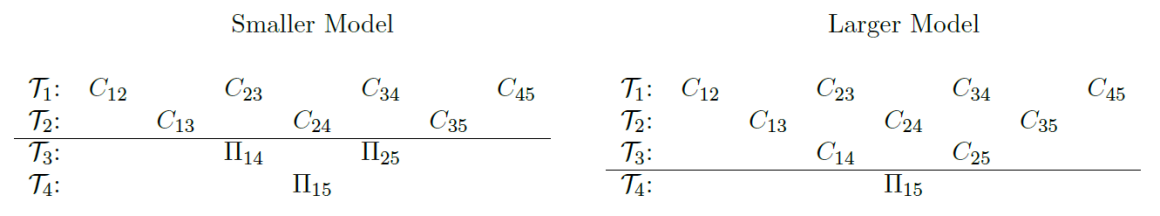
Figure 2: Graphical representation of truncated 5-dimensional D-vines.

The commonly used BIC is employed for bivariate copula selection in each tree. Specifically, given the $j$th insurance risk, for tree $k$ of the D-vine, we define the BIC-based model selection criterion for a candidate bivariate copula $C$ as

$$\text{BIC}_{k}^{(j)}=-2\sum_{i=1}^{n}\sum_{\begin{subarray}{c}1\leq s\leq T-k\\ t=s+k\end{subarray}}\log f\left(y^{(j)}_{is},y^{(j)}_{it}|y^{(j)}_{is+1},\ldots,y^{(j)}_{it-1};\bm{x}_{i}^{(j)}\right)+\log n\cdot(\text{number of parameters in }C),$$

where the likelihood function $f(y^{(j)}_{is},y^{(j)}_{it}|y^{(j)}_{is+1},\ldots,y^{(j)}_{it-1};\bm{x}_{i}^{(j)})$ can be readily evaluated based on the selected copulas $\{C_{s,t}^{(j)}\}_{t-s<k}$ of previous trees (i.e. tree 1 to tree $k-1$) and the current candidate copula $C$ for tree $k$ (see Algorithm 1 for more details). We select the bivariate copula in the candidate set that minimizes $\text{BIC}_{k}^{(j)}$.

We examine the performance of the sequential tree-by-tree selection procedure via extensive numerical experiments in Section LABEL:subsec:simu_copselection of the supplement, where it is seen to be computationally efficient and can accurately identify the true truncation order of the D-vine (i.e. the optimal weight given to historical observations for prediction) and the true bivariate copula for each tree.

5 Empirical Analysis

5.1 Data Description

Our dataset features bundled insurance risks from a multi-peril property insurance fund in the state of Wisconsin. The fund is established to provide property insurance for local government entities including counties, cities, towns, villages, school districts, fire departments, and other miscellaneous entities, and is administered by the Wisconsin Office of the Insurance Commissioner. The fund operates and functions as a stand-alone commercial property insurer in that it charges premiums and pays claims to its policyholders, i.e. local government units. On average, the fund writes approximately $25 million in premiums and $75 billion in coverage each year.

One major coverage that the fund provides to local government entities is building and contents, where the building element covers the physical structure of a property including its permanent fixtures and fittings, and the contents element covers possessions and valuables within the property that are detached and removable. It is an open-peril policy such that the policy insures against loss to covered properties from all causes with certain exclusions. Such exclusions include those resulting from flood, earthquake, wear and tear, extremes in temperature, mold, war, nuclear reactions, and embezzlement or theft by an employee. The fund groups all perils into three categories: water, fire, and others. Each category represents an insurance risk and there are $J=3$ bundled risks associated with a single insurance policy. The measurement of insurance risks is the number of claims per year. The dataset contains detailed policyholder-level information, including exogenous predictors and claim history, for 1019 local government entities over a six-year period from 2006-2011.

To conserve space, we provide detailed description of the dataset, including descriptive statistics of the exogenous predictors and the multivariate longitudinal claim counts, and sample dependence measures, in Section LABEL:sec:moreresults of the supplementary material. In the empirical analysis conducted in Sections 5-6, we use the observations in years 2006-2010 as the training data to develop the D-vine based predictive model (i.e. we have $n=1019$ and $T=5$ for model estimation) and use the data in year 2011 as the hold-out sample for model validation and comparison.

5.2 Model Specification and Estimation

To analyze the claim count of each peril (water, fire, and other), we consider the zero-one inflated negative binomial regression (8) proposed in Section 3.2. In addition, we examine its nested and limiting cases, including standard Poisson and negative binomial regression, and the count regression models with inflation only in zero and one respectively.

To assess the goodness-of-fit, we compare the empirical claim frequency with the frequency implied from the fitted regression model, which is calculated as the sum of the estimated probabilities of claim count over all policyholders at each observed value. The count regression model is then selected for each peril based on the chi-squared statistics. We refer to Table LABEL:tab:count in Section LABEL:sec:moreresults of the supplementary material for more details on the empirical claim frequency of each peril. Table 1 reports the goodness-of-fit statistics for the selected model as well as the alternative candidates. For the peril of water, fire, and others, we select the zero-one inflated negative binomial model (ZOINB), standard negative binomial model (NB), and one inflated negative binomial model (OINB), respectively.

The claim counts from all perils exhibit strong evidence of overdispersion that cannot be well-captured by Poisson-based models, a feature commonly observed in insurance claim data. Since insurance operation is based on risk pooling, the overdispersion in claim counts is usually attributed to the excess of zeros corresponding to the large number of policyholders without any claims. An interesting finding for the peril-wise claim count data in our study is, in addition to the zero inflation, there is a significant portion of ones as evidenced by the selected count regression models for the water and other perils.

Table 1: Goodness-of-fit statistics of different count regression models for claim count by peril. Z,O,I,P,NB stands for zero, one, inflated, Poisson and negative binomial, respectively.

			Alternative Models
Peril	Selected Model		Poisson	ZIP	ZOIP
Water	ZOINB	24.604	151.139	61.891	39.489
Fire	NB	8.178	63.953	8.945	8.945
Other	OINB	26.734	100.393	81.211	48.520

The estimation results for the selected count regression models are given in Table 2. We refer to Table LABEL:tab:covariates in Section LABEL:sec:moreresults of the supplementary material for more details on the exogenous predictors used in the regression. Some observations are as follows. There exists significant difference in claim frequency across different entity types (City, County, School, Town, Village), though the effects are heterogeneous across the three perils. The alarm credit (AC05, AC10, AC15) is not predictive regardless of the peril type, which is intuitively understandable as the alarm system is a more effective tool for loss control rather than loss prevention. The amount of coverage of the insurance policy shows substantial predictive power for all perils, indicating it is a sensible measure of risk exposure for the policyholder.

Table 2: Estimation results of count regression models for claim count by peril. For exogenous predictors: (a) City, County, School, Town, Village are entity type indicators; (b) AC05, AC10, AC15 are alarm credit indicators; (c) Coverage is the amount of coverage of the insurance policy.

	Water			Fire			Other
	EST.	S.E.		EST.	S.E		EST.	S.E
Intercept	-5.985	0.365		-3.987	0.229		-5.276	0.401
City	1.270	0.318		1.072	0.216		0.739	0.340
County	0.570	0.341		1.622	0.223		0.974	0.350
School	-0.273	0.321		0.170	0.217		0.299	0.338
Town	1.767	0.450		0.093	0.326		0.325	0.593
Village	1.381	0.332		1.047	0.221		0.690	0.364
AC05	-0.166	0.338		0.098	0.228		0.324	0.312
AC10	-0.099	0.273		0.276	0.179		0.107	0.285
AC15	0.065	0.144		0.141	0.102		0.086	0.158
Coverage	1.225	0.061		0.477	0.036		0.808	0.057
$\phi$	0.279	0.044		1.142	0.177		0.370	0.062
Zero Model
Intercept	-4.175	1.452
Coverage	0.495	0.204
One Model
Intercept	-3.356	0.152					-4.254	0.268
Coverage	0.159	0.055					0.316	0.072

For the dependence model, we employ the pair copula construction with D-vine to accommodate the temporal dependence for longitudinal measurements of each peril. The tree-by-tree sequential selection procedure proposed in Section 4.2 is used to automatically select the bivariate copulas for each D-vine, and we consider a candidate set of bivariate copulas that contains the most widely used copulas in practice, including the Independence, Gaussian, Frank, (rotated) Clayton, (rotated) Gumbel, and (rotated) Joe copulas. Given the selected bivariate copulas for each D-vine, we estimate the model parameters using the three-stage MLE described in Section 4.1.

The selected bivariate copulas and the estimated model parameters for the three D-vines are reported in Table 3. To better gauge the magnitude of the dependence, we further present the Kendall’s $\tau$ implied by the bivariate copulas. Some observations are as follows. First, a wide range of bivariate copulas are selected for each D-vine, which confirms that D-vine can accommodate flexible temporal dependence. Second, the estimated temporal dependence is positive, implying the imperfection of the insurer’s risk classification system. This further foreshadows the important role of the predictive model in improving the insurance operations (Section 6). Third, within each D-vine, the estimated dependence of bivariate copulas decreases from the top to the bottom trees. The diminishing dependence pattern is consistent with the fundamental idea of the graphical model in that pairs in higher level trees are conditioned on a larger set of correlated variables, and thus are expected to be less dependent. In particular, note that the D-vines for both water and other perils are truncated (i.e. conditional independence beyond a certain tree level), with the former at the third tree and the latter at the second tree, indicating that the optimal credibility weights given to historical claim counts data are different across the three perils.

Table 3: Selected bivariate copulas and its estimated model parameters (Est.) and Kendall’s $\tau$ in each D-vine by peril. Standard errors are presented in parenthesis. R. stands for Rotated. $T_{k}$ denotes the $k$th tree for $k=1,\cdots,4$.

	Water				Fire				Other
	Copula	Est.	$\tau$		Copula	Est.	$\tau$		Copula	Est.	$\tau$
$T_{1}$	R.Gumbel	1.547	0.359		R.Gumbel	1.299	0.222		Clayton	0.920	0.315
		(0.054)				(0.045)				(0.170)
$T_{2}$	R.Gumbel	1.321	0.246		R.Gumbel	1.312	0.231		R.Gumbel	1.252	0.201
		(0.053)				(0.052)				(0.057)
$T_{3}$	Frank	1.529	0.166		R.Gumbel	1.216	0.179
		(0.342)				(0.056)
$T_{4}$					R.Clayton	0.172	0.080
						(0.052)

The contemporaneous dependence among the three perils are captured using a Gaussian copula with an unstructured dispersion matrix. The estimated pairwise association parameters are reported in Table 4, where significant dependence is observed among the three types of risks. The results support the unstructured association across claim counts from different perils and are consistent with the observations in Figure LABEL:fig:corcount of the supplementary material. We remark that the proposed framework allows alternative copula specifications of $C_{J}$ to capture the contemporaneous dependence among the multivariate insurance risks, such as factor copulas and hierarchical Archimedean copulas. In our current study, the Gaussian copula is a favorable choice due to its balance between interpretability and computational difficulty. Moreover, our analysis shows that the Gaussian copula sufficiently captures the association among insurance claim counts of different perils.

Table 4: Estimates of pairwise contemporaneous dependence among perils

	Water-Fire	Water-Other	Fire-Other
Estimate	0.126	0.199	0.070
$t$-stat	3.558	5.083	1.887

5.3 Model Validation

Business decisions in insurance operations are often based on the forecast of risk outcomes in the future period. To reflect the uncertainty of the future, any prediction should be treated as probabilistic, i.e. they should take form of probability distributions over future quantities. Hence, we perform model validation for the predictive distribution (1) instead of point prediction, and we examine the predictive performance of the proposed model using the proper scoring rules for probabilistic forecasts (Gneiting and Raftery,, 2007; Czado et al.,, 2009).

Our validation procedure is based on the aggregate risk $S_{i,T+1}$ defined in (2). Without loss of generality, we set $\alpha_{i,T+1}^{(j)}=1$ for $j\in\{1,\ldots,J\}$ and $i\in\{1,\ldots,n\}$ for simplicity. Thus $S_{i,T+1}$ is the total number of claims from all perils for the $i$th policyholder in the future period $T+1$ (i.e. year 2011). Let $F_{S}(\cdot|\bm{H}_{iT})$ denote the predictive distribution of $S_{i,T+1}$ conditional on history $\bm{H}_{iT}$, i.e.,

$$F_{S}(s|\bm{H}_{iT}) ={\rm Pr}(S_{i,T+1}\leq s|\bm{H}_{iT})=\sum_{\left\{\left(y_{i,T+1}^{(1)},\cdots,y_{i,T+1}^{(J)}\right)\middle|S_{i,T+1}\leq s\right\}}f\left(y^{(1)}_{i,T+1},\ldots,y^{(J)}_{i,T+1}|H_{iT}^{(1)},\ldots,H_{iT}^{(J)}\right).$$

Note that $f(y^{(1)}_{i,T+1},\ldots,y^{(J)}_{i,T+1}|H_{iT}^{(1)},\ldots,H_{iT}^{(J)})$ can be obtained from the predictive model (1) as

$$f\left(y^{(1)}_{i,T+1},\ldots,y^{(J)}_{i,T+1}|H_{iT}^{(1)},\ldots,H_{iT}^{(J)}\right)$$

$$= \sum_{k_{1}=0}^{1}\cdots\sum_{k_{J}=0}^{1}(-1)^{k_{1}+\cdots+k_{J}}F\left(y^{(1)}_{i,T+1}-k_{1},\ldots,y^{(J)}_{i,T+1}-k_{J}|H_{iT}^{(1)},\ldots,H_{iT}^{(J)}\right),$$

and as discussed in Section 3.3, $F(y^{(1)}_{i,T+1},\ldots,y^{(J)}_{i,T+1}|H_{iT}^{(1)},\ldots,H_{iT}^{(J)})=F(\bm{y}_{i,T+1}|\bm{H}_{i,T})$ and can be evaluated efficiently via Algorithm 1 by setting $t=T+1$.

Given the predictive distribution $\{F_{S}(\cdot|\bm{H}_{iT})\}_{i=1}^{n}$ given by the model, the validation is based on the probability integral transformation (PIT) of $\{S_{i,T+1}\}_{i=1}^{n}$. It is well-known that for a continuous random variable $Z$ with cdf $F_{Z}(\cdot)$, the PIT $F_{Z}(Z)$ is a uniform random variable. For the portfolio of policyholders, denote $s_{i,T+1}$ as the realized value of $S_{i,T+1}$ and define $u_{i,T+1}=F_{S}(s_{i,T+1}|\bm{H}_{iT})$. Therefore, the validity of the predictive model can be empirically tested by examining whether $\{u_{i,T+1};i=1,\cdots,n\}$ is a random sample from the uniform distribution.

However, in our context, $S_{i,T+1}$ represents the number of claims at the policy level. Due to the discrete nature of $S_{i,T+1}$, the standard PIT is not applicable. To address this issue, we instead consider a randomized PIT defined by (see Rüschendorf, (2009)):

$$U_{i}=F_{S}(S_{i,T+1}-1|\bm{H}_{iT})+V_{i}\cdot(F_{S}(S_{i,T+1}|\bm{H}_{iT})-F_{S}(S_{i,T+1}-1|\bm{H}_{iT})),$$

where $V_{i}$ is i.i.d. uniform random variable and we define $F_{S}(-1|\bm{H}_{iT})=0$ for $i=1,\cdots,n$. In addition, we consider a nonrandomized PIT which is defined based on the conditional CDF of $U_{i}$ given the observed claim count $S_{i,T+1}=s_{i,T+1}$ (see Section 2.1 in Czado et al., (2009) for more details). The randomized and nonrandomized PIT histograms are exhibited in Figure 3. Both transformations are uniformly distributed, suggesting the predictive distribution based on the proposed D-vine model is well calibrated. The uniformity is formally tested using the Kolmogorov-Smirnov (KS) statistics for both randomized and nonrandomized PITs. For the randomized PIT, the KS statistic is 0.0307, which gives a $p$-value of 0.294. For the nonrandomized PIT, the KS statistic is 0.0326, which gives a $p$-value of 0.199. The result provides further support that the predictive distribution based on the D-vine model is sufficiently flexible for insurance applications.

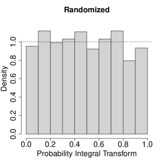
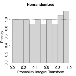
Figure 3: PIT histograms based on the predictive distribution.

To further illustrate the importance of dependence modeling for prediction, we further compare the predictive accuracy between the proposed D-vine model and the independence model, which ignores the temporal and contemporaneous dependence among multivariate bundled insurance risks.

The assessment is again based on the predictive distribution of $S_{i,T+1}$. We employ consistent scoring rules to evaluate the sharpness/accuracy of the predictive distribution estimated by the two models. Specifically, we consider three scoring rules introduced in Czado et al., (2009), the ranked probability score (RPS), the quadratic score (QS), and the spherical score (SPHS), which essentially quantify the closeness between the realized value $s_{i,T+1}$ in the hold-out sample and the predictive distribution $F_{S}(\cdot|\bm{H}_{iT})$ estimated based on training data. All scores are negatively oriented, i.e., the lower the score, the more accurate the prediction. The three scores are calculated for each of the 1019 policyholders for both the independence model and the D-vine model. Table 5 reports the empirical probability that the D-vine model outperforms the independence model. The dependence-aware prediction based on the D-vine model is superior to the independence model for about 70% of policyholders in the hold-out sample across all three scoring rules. The large $Z$-scores for the one-sided binomial tests further confirm the statistical significance of the result.

Table 5: Empirical probability of superior prediction by the D-vine model

	RPS	QS	SPHS
Estimate	69.09%	68.40%	68.99%
$Z$-score	12.19	11.74	12.12

6 Managerial Implications on Key Insurance Operations

This section illustrates in detail the prominent managerial implications of the proposed D-vine predictive model, in particular, the dependence among multivariate longitudinal insurance risks, on several key insurance operations outlined in Section 2.

We emphasize that current modeling practice in the insurance industry mostly generates prediction for bundled insurance risks without accounting for any dependence or only accounts for temporal dependence. In contrast, the D-vine predictive model enables simultaneous analysis of both temporal and contemporaneous dependence, and thus generates fully dependence-aware prediction. We show below that the dependence-aware prediction significantly improves the insurer’s profitability in risk pricing and provides more accurate risk assessment for reinsurance.

We consider the standard scenario where business decisions are made based on the prediction of future aggregate loss of individual policyholders. Specifically, given historical information on an insurance portfolio over the past $T$ years, the insurer is to make operational decisions based on the prediction for year $T+1$. A policyholder’s aggregate loss in year $T+1$ is defined in (2) and we derive the average cost per claim via a generalized linear model (GLM). Specifically, we fit a Gamma GLM using data in the first $T$ years, where the response variable is the average cost per claim and the predictors are summarized in Table LABEL:tab:covariates of Section LABEL:sec:moreresults of the supplementary material. See de Jong and Heller, (2008) for implementation of GLMs for insurance data. A GLM is fitted separately for each peril, and the predicted outcome for year $T+1$ is used as the average cost per claim in the following analysis.

6.1 Risk Segmentation and Pricing

We first examine the insurer’s underwriting and ratemaking practice. To identify profitable business, it is essential for the insurer to conduct risk segmentation, i.e. separating high risk and low risk customers. For this purpose, the expected loss cost in year $T+1$ defined in (3) is commonly used by the insurer as a risk score to rank and select policyholders. To better illustrate the effects and importance of both temporal and contemporaneous dependence, we conduct analysis for two types of insurance contracts, one without deductibles and one with deductibles.

Insurance contracts without deductibles: Under the case of zero deductibles $d=0$, we have $\eqref{equ:exprate}=\sum_{j=1}^{J}\alpha_{i,T+1}^{(j)}\mathbb{E}(y^{(j)}_{i,T+1}|H_{iT}^{(1)},\ldots,H_{iT}^{(J)}).$ In other words, the expected total loss of the bundled insurance contract can be decomposed into summation of loss cost of each risk. Under such scenario, the temporal dependence within each insurance risk plays an essential role in generating accurate prediction of risk scores of the insurance policy (i.e. expected loss cost in (3)).

We compare two risk scores, one generated by the independence model which ignores dependence among insurance risks (denoted by $\pi_{ind}$), and one generated by the proposed D-vine model (denoted by $\pi_{dep}$). Note that the difference between $\pi_{ind}$ and $\pi_{dep}$ is mainly due to temporal dependence, as the expected total loss cost can be decomposed into summation of expected loss from each peril.

We employ the ordered Lorenz curve (see Frees et al., (2012)) to assess the out-of-sample performance of the two risk scores in the hold-out sample and demonstrate the importance of temporal dependence within insurance risks. Recall that $\bm{H}_{iT}=(H_{iT}^{(1)},\ldots,H_{iT}^{(J)})$ denotes historical data observed up to period $T$. Let $R_{i,T+1}=R(\bm{H}_{iT})$ be a relativity derived based on $\bm{H}_{iT}$ that the insurer uses to rank individual policyholders, and define $R_{i,T+1}=q_{i,T+1}/p_{i,T+1}$ where $p_{i,T+1}=p(\bm{H}_{iT})$ is a base score that can be interpreted as the premium, and $q_{i,T+1}=q(\bm{H}_{iT})$ is an alternative score that challenges the base. The empirical ordered Lorenz curve describes the relation between $G_{L}(u)$ and $G_{P}(u)$ which are defined as:

$$G_{L}(u)=\frac{\sum_{i=1}^{n}s_{i,T+1}\mathbb{I}(R_{i,T+1}\leq u)}{\sum_{i=1}^{n}s_{i,T+1}}~{}~{}{\rm and}~{}~{}G_{P}(u)=\frac{\sum_{i=1}^{n}p_{i,T+1}\mathbb{I}(R_{i,T+1}\leq u)}{\sum_{i=1}^{n}p_{i,T+1}}.$$

Note that we can interpret $R_{i,T+1}\leq u$ as the $i$th policyholder being selected for renewal during underwriting, and thus $G_{L}$ and $G_{P}$ can be interpreted as the proportion of losses and premiums of the selected risks at the future period $T+1$.

For the purpose of risk segmentation, we employ the constant premium as the base score, i.e. $p_{i,T+1}=1$, and examine which of the two alternative scores $\pi_{ind}$ and $\pi_{dep}$ better identifies profitable portfolio. The corresponding ordered Lorenz curves are shown in the left panel of Figure 4. Both curves are below the equity line (i.e. diagonal), indicating substantial opportunities for risk segmentation. For instance, at the 80% premium level, the proportions of losses of selected contracts are about 30% and 25% when using $\pi_{ind}$ and $\pi_{dep}$ for risk segmentation respectively. In addition, there is no crossing between the two ordered Lorenz curves, which suggests that the risk score $\pi_{dep}$ better identifies additional profitable business at every possible underwriting strategy than $\pi_{ind}$. We further summarize the overall performance of the risk score using the associated Gini index calculated as $Gini=1-2\int_{0}^{\infty}G_{L}(u)dG_{P}(u)$. Graphically speaking, the Gini index is twice the area between the ordered Lorenz curve and the equity line, and thus can be interpreted as average profit over all underwriting strategies. The Gini indices associated with scores $\pi_{ind}$ and $\pi_{dep}$ are 63.97% and 69.44% respectively. Thus, appropriate modeling of temporal dependence within each insurance risk provides about 9% increase in the insurer’s profitability.

Furthermore, an insurer can use the ordered Lorenz curve to identify unprofitable business and thus exercises ratemaking to further improve its profitability. In ratemaking, the goal is to set a new insurance premium rate. We show that an insurer can use the risk scores to suggest change to the base premium. For this purpose, we let each of the scores $\pi_{ind}$ and $\pi_{dep}$ serve as the base premium, and the other serve as the challenger. The corresponding Lorenz curves are presented in the right panel of Figure 4. In the first case, when $\pi_{ind}$ is the base premium, we observe that the ordered Lorenz curve is below the equity line. This suggests that by switching from the base premium $\pi_{ind}$ to the new premium $\pi_{dep}$, the insurer could better separate high risk and low risk, and thus generate higher profit margin. In contrast, when $\pi_{dep}$ is the base premium, the resulting ordered Lorenz curve lies above the equity line, which corresponds to unprofitable business.

Table 6 reports the Gini indices associated with Figure 4 (right panel). The first row corresponds to the solid line where we use $\pi_{ind}$ as the base premium and use $\pi_{dep}$ as the challenger to create relativity. As confirmed by the positive Gini index, switching from $\pi_{dep}$ to $\pi_{ind}$ for ratemaking results in notable improvement of the insurer’s profitability. The second row corresponds to the dashed line where we use $\pi_{dep}$ as the base premium and use $\pi_{ind}$ to create relativity, which hurts the profit as indicated by the negative Gini index. The standard errors in both cases suggest that we can use $\pi_{dep}$ as the new premium rate with confidence.

Figure 4: Ordered Lorenz curves for comparing risk scores $\pi_{ind}$ and $\pi_{dep}$ without deductibles. The left panel corresponds to risk segmentation, and the right panel corresponds to ratemaking.

Table 6: Gini indices for ratemaking without deductibles. Standard errors are in parentheses.

Base	Challenger
	Independence		Dependence
Independence			49.070 (10.982)
Dependence	-28.317 (13.287)

To summarize, our analysis shows the importance of modeling temporal dependence within each insurance risk for achieving profitable risk segmentation and pricing in insurance contracts without deductibles. We note that a similar analysis was previously conducted in Shi and Yang, (2018), where the authors studied temporal dependence for univariate longitudinal data of claim amount and demonstrated its practical value. In comparison, our analysis models temporal dependence for longitudinal data of claim count. Therefore, the two studies complement each other and provide empirical evidence from different angles for the importance of temporal dependence in risk segmentation and pricing.

Insurance contracts with deductibles: An insurance contract often features risk retention measures such as deductible and coverage limit (see e.g. Lee, (2017)). In particular, deductible is the most common risk retention method that property insurers use to share risks with policyholders. In the following, we consider ratemaking with deductibles and demonstrate the critical role of both temporal and contemporaneous dependence among multivariate longitudinal insurance risks in correctly pricing bundled insurance contracts with deductibles.

We consider an annual deductible $d>0$ which is often found in property insurance and health insurance. Recall from (3) that with a deductible $d$, the expected total loss cost of the insurer for the $i$th policyholder is $\mathbb{E}((S_{i,T+1}-d)_{+}|H_{iT}^{(1)},\ldots,H_{iT}^{(J)})$. Note that the $(\cdot)_{+}$ operator prevents the decomposition of the total loss into summation of loss cost of each risk. Thus, for an insurance contract with deductibles, we need to calculate its risk score directly from (3).

We examine two risk scores. The first score is derived from a D-vine based predictive model which only accounts for temporal dependence within each risk (i.e. we set the multivariate copula $C^{J}$ as an independence copula). This score serves as a proxy for the common practice in the insurance industry for pricing bundled insurance risks. The second score is generated by the proposed D-vine model with both temporal and contemporaneous dependence. A comparison between the two scores highlights the managerial significance of simultaneous analysis of both temporal and contemporaneous dependence on improving decision making of insurers for deductible ratemaking.

Same as before, we evaluate the out-of-sample ratemaking performance of the two risk scores using the ordered Lorenz curve and the associated Gini index. In particular, we focus on the base-challenger analysis as discussed before, where we use one score as the base premium and use the alternative score as the challenger to create relativity. We test whether switching to the alternative score allows the insurer to better separate low and high risks and improve ratemaking.

We consider three different levels of deductibles for the insurance policy with $d$=15K, 20K and 25K. The resulting ordered Lorenz curves and the Gini indices are given in Figure 5 and Table 7 respectively. When the risk score accounting for only temporal dependence is used as the base premium, the Gini indices are positive across all deductible levels, suggesting more profitable ratemaking for the insurer when looking to the alternative score. On the contrary, if the base premium takes into account both temporal and contemporaneous dependence, by switching to the alternative score, the insurer is subject to ratemaking losses as implied by the negative Gini index. In summary, this analysis shows that on top of the temporal dependence, contemporaneous dependence provides additional lift for the insurer to identify profitable business, indicating the importance of simultaneous analysis of both temporal and contemporaneous dependence.

Figure 5: Ordered Lorenz curves for ratemaking at different deductible levels.

Table 7: Gini indices for ratemaking with deductibles. Standard deviations are in parentheses.

Base	Challenger
	Temporal Dep. Only				Complete Dependence
	15K	20K	25K		15K	20K	25K
Temporal Dep. Only					23.140	30.530	38.060
					(3.586)	(3.568)	(3.632)
Complete Dependence	-21.910	-27.650	-34.240
	(3.605)	(3.620)	(3.736)

6.2 Risk Management: Portfolio Reinsurance

In this section, we discuss the application of the D-vine predictive model in portfolio risk management. Risk segmentation and pricing concerns business decisions for individual insurance contracts. In contrast, risk management decisions are made from the viewpoint of an insurance portfolio.

The maximum amount of liability that an insurer could assume determines its underwriting capacity. Quota share reinsurance is a commonly used approach for an insurer to transfer risks to a reinsurance company and thus maintain its underwriting capacity for profitable business. Through reinsurance, the insurer reduces its liability and ensures its ability to pay out claims to policyholders when needed, and thus avoids insolvency.

Under quota share reinsurance, the retained risk by the insurer is given by (4). The insurer’s goal is to determine the optimal retention quota $\delta_{i}$ for each contract $i=1,\cdots,n$ in its insurance portfolio. From the insurer’s perspective, the optimal retention $\{\delta_{i}\}_{i=1}^{n}$ can be solved via an optimization such that:

$$\{\delta_{i}\}_{i=1}^{n}=\operatorname*{arg\,min}{\rm Var}(S_{T+1}^{*}|H_{1},\ldots,H_{T})~{}~{}s.t.~{}~{}{\mathbb{E}}(S_{T+1}^{*}|H_{1},\ldots,H_{T})=K,$$ (13)

where $S_{T+1}^{*}=\sum_{i=1}^{n}\delta_{i}S_{i,T+1}$ as defined in (4), $H_{t}=\{H_{it}^{(j)}:j\in\{1,\ldots,J\},i\in\{1,\ldots,n\}\}$, and $K$ is a constant representing the target revenue of the insurer and is determined by its underwriting capacity. Essentially, the insurer finds the optimal retention $\{\delta_{i}\}_{i=1}^{n}$ by minimizing the volatility of the retained portfolio risk while maintaining a target revenue. Straightforward calculation via the Lagrange multiplier gives that the optimal retention quota for the $i$th contract is

$$\delta_{i}\propto\frac{{\mathbb{E}}(S_{i,T+1}|\bm{H}_{iT})}{{\rm Var}(S_{i,T+1}|\bm{H}_{iT})}\text{ for }i=1,\cdots,n.$$ (14)

Thus, the optimal quota $\delta_{i}$ is determined by the conditional distribution of $S_{i,T+1}$, which in turn depends on both temporal and contemporaneous dependence of the bundled insurance risks.

We compare the performance of two predictive models. The first is a D-vine based predictive model that only accounts for temporal dependence within each risk. This serves as a proxy for the current modeling practice in the insurance industry. The second is the proposed D-vine model which simultaneously accounts for both temporal and contemporaneous dependence.

Based on either predictive model, for any fixed target revenue $K$, the insurer can estimate the optimal retention quota $\{\delta_{i}\}_{i=1}^{n}$ via (14). In the left panel of Figure 6, we show the violin plot of $\{\delta_{i}\}_{i=1}^{n}$ estimated via the predicted D-vine model that accounts for both types of dependence at selected levels of target revenue $K$. It is intuitive to observe that larger target revenue $K$ is associated with higher retention quota $\{\delta_{i}\}_{i=1}^{n}$ of the insurance risk. Denote $\{\delta_{i}^{\prime}\}_{i=1}^{n}$ as the optimal retention quota estimated via the predictive model with only temporal dependence. To illustrate the impact of contemporaneous dependence, the right panel of Figure 6 gives the histogram of the percentage bias $\{(\delta_{i}^{\prime}-\delta_{i})/\delta_{i}\times 100\%\}_{i=1}^{n}$ of retained quota estimated from the predictive model with only temporal dependence. As can be seen, ignoring contemporaneous dependence generally results in notable (upward) bias of the estimated retention quota (see more discussions later).

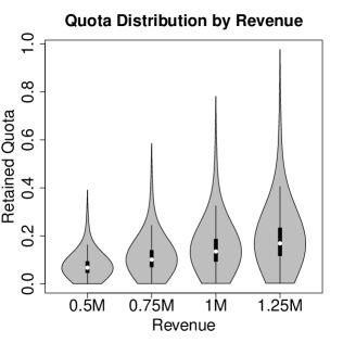
Figure 6: The left panel corresponds to optimal retention quota estimated via the proposed D-vine model. The right panel corresponds to the percentage bias of retention quota caused by the predictive model with only temporal dependence (i.e. ignoring contemporaneous dependence).

Given $\{\delta_{i}\}_{i=1}^{n}$, the insurer can further estimate the volatility of the retained insurance portfolio. The curves in Figure 7 visualize the relationship between the estimated volatility (uncertainty) of the optimal retained portfolio and the target revenue $K$ derived based on the two predictive models. As expected, one observes the risk-return trade-off for each curve, i.e. with higher underwriting capacity $K$ to assume more business, the insurer undertakes a higher uncertainty in the retained insurance portfolio.

More importantly, Figure 7 illustrates the significant effect of the dependence among bundled insurance risks on the reinsurance operation. Note that the estimated volatility of the retained portfolio given by the proposed D-vine model (solid line) is always higher than the volatility estimated by the predictive model with only temporal dependence (dashed line). In fact, the divergence between the two curves corresponds to a 9.83% underestimation of the volatility by the latter model. This is indeed not surprising as recall that the multivariate claim counts (and thus the insurance risks) from the three perils are positively dependent as found in Section 5.2 (Table 4), a phenomenon commonly seen among bundled insurance risks. Thus ignoring the contemporaneous dependence in predictive modeling results in an underestimation of the uncertainty in the retained insurance portfolio, which could lead to disastrous scenarios such as insolvency of the insurer. In summary, this analysis again indicates the managerial significance of simultaneous analysis of both temporal and contemporaneous dependence for insurance operations related to bundled risks.

Figure 7: Effects of dependence among bundled insurance risks on risk retention under reinsurance.

7 Conclusion

In this work, we proposed a D-vine based predictive modeling framework for insurers to manage multivariate insurance risks embedded in insurance policies with bundling features. The proposed framework utilized pair copula construction to allow for simultaneous modeling of the temporal and contemporaneous dependence among multivariate longitudinal insurance risks. Using a dataset on a commercial insurer’s portfolio of bundled property insurance policies, we demonstrated the prominent managerial significance of the dependence-aware prediction based on the proposed model. Our work made a methodological contribution to the modeling and analysis of multivariate longitudinal data. Though our analysis focused on the claim count of policyholders, the application of the proposed framework is much broader in that it easily accommodates measurements of various types, be it discrete, semi-continuous, or continuous, and it further allows the multivariate outcomes to be measured in different scales, for instance, a mix of both discrete and continuous outcomes.

In the proposed predictive model, we emphasize two types of dependence among insurance risks, the temporal association within each risk and the contemporaneous dependence across multiple risks. To highlight the managerial implications, we considered two key operations, risk pricing and risk management, that are essential to the insurance business. We showed that dependent risks could have significant impact on the insurer’s profitability and on the uncertainty of the insurance portfolio. More importantly, we showed that carefully accounting for the dependence among insurance risks can substantially improve the current practice in the insurance industry. This is of significant practical values, as insurance is an essential sector in any developed economy.

References

- Aas et al., (2009) Aas, K., Czado, C., Frigessi, A., and Bakken, H. (2009). Pair-copula constructions of multiple dependence. Insurance: Mathematics and Economics, 44(2):182–198.
- Albrecher et al., (2017) Albrecher, H., Beirlant, J., and Teugels, J. L. (2017). Reinsurance: actuarial and statistical aspects. John Wiley & Sons.
- Barthel et al., (2018) Barthel, N., Geerdens, C., Killiches, M., Janssen, P., and Czado, C. (2018). Vine copula based likelihood estimation of dependence patterns in multivariate event time data. Computational Statistics & Data Analysis, 117:109–127.
- Beare, (2010) Beare, B. (2010). Copulas and temporal dependence. Econometrica, 78(1):395–410.
- Bedford and Cooke, (2001) Bedford, T. and Cooke, R. M. (2001). Probability density decomposition for conditionally dependent random variables modeled by vines. Annals of Mathematics and Artificial intelligence, 32(1):245–268.
- Bedford and Cooke, (2002) Bedford, T. and Cooke, R. M. (2002). Vines–a new graphical model for dependent random variables. Annals of Statistics, 30(4):1031–1068.
- Bernard et al., (2014) Bernard, C., Jiang, X., and Wang, R. (2014). Risk aggregation with dependence uncertainty. Insurance: Mathematics and Economics, 54:93–108.
- Boucher and Inoussa, (2014) Boucher, J.-P. and Inoussa, R. (2014). A posteriori ratemaking with panel data. ASTIN Bulletin: The Journal of the International Actuarial Association, 44(3):587–612.
- Brechmann and Czado, (2015) Brechmann, E. C. and Czado, C. (2015). COPAR–multivariate time series modeling using the copula autoregressive model. Applied Stochastic Models in Business and Industry, 31(4):495–514.
- Brechmann et al., (2012) Brechmann, E. C., Czado, C., and Aas, K. (2012). Truncated regular vines in high dimensions with application to financial data. Canadian Journal of Statistics, 40(1):68–85.
- Brockwell and Davis, (1991) Brockwell, P. J. and Davis, R. A. (1991). Time Series: Theory and Methods. Springer New York.
- Bühlmann and Gisler, (2005) Bühlmann, H. and Gisler, A. (2005). A Course in Credibility Theory and its Applications. Springer.
- (13) Chen, X. and Fan, Y. (2006a). Estimation and model selection of semiparametric copula-based multivariate dynamic models under copula misspecification. Journal of Econometrics, 135(1–2):125–154.
- (14) Chen, X. and Fan, Y. (2006b). Estimation of copula-based semiparametric time series models. Journal of Econometrics, 130(2):307–335.
- Chen et al., (2021) Chen, X., Huang, Z., and Yi, Y. (2021). Efficient estimation of multivariate semi-nonparametric garch filtered copula models. Journal of Econometrics, 222(1):484–501.
- Chen et al., (2009) Chen, X., Wu, W. B., and Yi, Y. (2009). Efficient estimation of copula-based semiparametric markov models. The Annals of Statistics, 37(6B):4214–4253.
- Czado et al., (2009) Czado, C., Gneiting, T., and Held, L. (2009). Predictive model assessment for count data. Biometrics, 65(4):1254–1261.
- de Jong and Heller, (2008) de Jong, P. and Heller, G. (2008). Generalized Linear Models for Insurance Data. Cambridge University Press.
- Denuit et al., (2007) Denuit, M., Maréchal, X., Pitrebois, S., and Walhin, J.-F. (2007). Actuarial Modelling of Claim Counts: Risk Classification, Credibility and Bonus-Malus Systems. John Wiley & Sons.
- Farewell et al., (2017) Farewell, V., Long, D., Tom, B., Yiu, S., and Su, L. (2017). Two-part and related regression models for longitudinal data. Annual review of statistics and its application, 4:283–315.
- Frees and Valdez, (2008) Frees, E. and Valdez, E. (2008). Hierarchical insurance claims modeling. Journal of the American Statistical Association, 103(484):1457–1469.
- Frees, (2015) Frees, E. W. (2015). Analytics of insurance markets. Annual Review of Financial Economics, 7:253–277.
- Frees et al., (2012) Frees, E. W., Meyers, G., and Cummings, A. D. (2012). Summarizing insurance scores using a gini index. Journal of the American Statistical Association, 106(495).
- Frees and Wang, (2006) Frees, E. W. and Wang, P. (2006). Copula credibility for aggregate loss models. Insurance: Mathematics and Economics, 38(2):360–373.
- Frees et al., (1999) Frees, E. W., Young, V. R., and Luo, Y. (1999). A longitudinal data analysis interpretation of credibility models. Insurance: Mathematics and Economics, 24(3):229–247.
- Gneiting and Raftery, (2007) Gneiting, T. and Raftery, A. E. (2007). Strictly proper scoring rules, prediction, and estimation. Journal of the American Statistical Association, 102:359–378.
- Godambe, (1960) Godambe, V. P. (1960). An optimum property of regular maximum likelihood estimation. The Annals of Mathematical Statistics, pages 1208–1211.
- Jessup et al., (2020) Jessup, S., Boucher, J.-P., and Pigeon, M. (2020). On fitting dependent nonhomogeneous loss models to unearned premium risk. North American Actuarial Journal, page forthcoming.
- Joe, (2005) Joe, H. (2005). Asymptotic efficiency of the two-stage estimation method for copula-based models. Journal of Multivariate Analysis, 94(2):401–419.
- Joe, (2014) Joe, H. (2014). Dependence Modeling with Copulas. Chapman & Hall, New York.
- Joe and Kurowicka, (2011) Joe, H. and Kurowicka, D. (2011). Dependence Modeling: Vine Copula Handbook. World Scientific.
- Kurowicka and Cooke, (2006) Kurowicka, D. and Cooke, R. M. (2006). Uncertainty Analysis with High Dimensional Dependence Modelling. John Wiley & Sons.
- Lee, (2017) Lee, G. Y. (2017). General insurance deductible ratemaking. North American Actuarial Journal, 21(4):620–638.
- Newey and McFadden, (1994) Newey, W. K. and McFadden, D. (1994). Large sample estimation and hypothesis testing. In Handbook of Econometrics, volume 4, chapter 36, pages 2111–2245. Elsevier B.V.
- Oh and Patton, (2013) Oh, D. and Patton, A. (2013). Simulated method of moments estimation for copula-based multivariate models. Journal of the American Statistical Association, 108(502):689–700.
- Oh and Patton, (2017) Oh, D. and Patton, A. (2017). Modelling dependence in high dimensions with factor copulas. Journal of Business and Economic Statistics, 35(1):139–154.
- Oh et al., (2020) Oh, R., Shi, P., and Ahn, J. Y. (2020). Bonus-malus premiums under the dependent frequency-severity modeling. Scandinavian Actuarial Journal, 2020(3):172–195.
- Panagiotelis et al., (2012) Panagiotelis, A., Czado, C., and Joe, H. (2012). Pair copula constructions for multivariate discrete data. Journal of the American Statistical Association, 107(499):1063–1072.
- Patton, (2006) Patton, A. (2006). Modelling asymmetric exchange rate dependence. International Economic Review, 47(2):527–556.
- Pinquet, (2013) Pinquet, J. (2013). Experience rating in nonlife insurance. In Dionne, G., editor, Handbook of Insurance, pages 471–485. Springer.
- Rüschendorf, (2009) Rüschendorf, L. (2009). On the distributional transform, sklar’s theorem, and the empirical copula process. Journal of Statistical Planning and Inference, 139(11):3921–3927.
- Shi and Yang, (2018) Shi, P. and Yang, L. (2018). Pair copula constructions for insurance experience rating. Journal of the American Statistical Association, 113(521):122–133.
- Sklar, (1959) Sklar, A. (1959). Fonctions de répartition à n dimensions et leurs marges. Publications de l’Institut de Statistique de L’Université de Paris, 8:229–231.
- Smith, (2015) Smith, M. S. (2015). Copula modelling of dependence in multivariate time series. International Journal of Forecasting, 31(3):815–833.
- Stöber et al., (2015) Stöber, J., Hong, H. G., Czado, C., and Ghosh, P. (2015). Comorbidity of chronic diseases in the elderly: Patterns identified by a copula design for mixed responses. Computational Statistics & Data Analysis, 88:28–39.
- Verbeke et al., (2014) Verbeke, G., Fieuws, S., Molenberghs, G., and Davidian, M. (2014). The analysis of multivariate longitudinal data: A review. Statistical Methods in Medical Research, 23(1):42–59.
- Wang et al., (2019) Wang, R., Xu, Z. Q., and Zhou, X. Y. (2019). Dual utilities on risk aggregation under dependence uncertainty. Finance and Stochastics, 23(4):1025–1048.
- Zhao and Zhang, (2018) Zhao, Z. and Zhang, Z. (2018). Semiparametric dynamic max-copula model for multivariate time series. Journal of the Royal Statistical Society: Series B.