Quadrature Strategies for Constructing Polynomial Approximations

Abstract

Finding suitable points for multivariate polynomial interpolation and approximation is a challenging task. Yet, despite this challenge, there has been tremendous research dedicated to this singular cause. In this paper, we begin by reviewing classical methods for finding suitable quadrature points for polynomial approximation in both the univariate and multivariate setting. Then, we categorize recent advances into those that propose a new sampling approach and those centered on an optimization strategy. The sampling approaches yield a favorable discretization of the domain, while the optimization methods pick a subset of the discretized samples that minimize certain objectives. While not all strategies follow this two-stage approach, most do. Sampling techniques covered include subsampling quadratures, Christoffel, induced and Monte Carlo methods. Optimization methods discussed range from linear programming ideas and Newton’s method to greedy procedures from numerical linear algebra. Our exposition is aided by examples that implement some of the aforementioned strategies.

1 Introduction

Over the past few years there has been a renewed research effort aimed at constructing stable polynomial approximations: understanding their theoretical properties shin2016near ; zhou2015weighted ; shin2016nonadaptive ; seshadri2017effectively ; chkifa2015discrete ; migliorati2015analysis ; cohen2013stability ; hampton2015coherence ; adcock2018approximating and extending their practical use. The latter spans from applications in spectral methods trefethen2000spectral , uncertainty quantification and the related sensitivity analysis pettersson2015polynomial ; seshadri2014leakage ; ghisu2017asme ; gmd-2017-107 to dimension reduction seshadri2018turbomachinery and design under uncertainty seshadri2016density . One topic germane to the field has been to find suitable points for multivariate polynomials using as few points as possible. The application-centric high level idea can be described as follows:

$$\begin{array}[]{c}\text{select a polynomial basis}\\ \Downarrow\\ \text{evaluate model at quadrature points }\\ \Downarrow\\ \textrm{estimate polynomial coefficients}\\ \Downarrow\\ \textrm{compute moments, sensitivities and probability density functions}\end{array}$$

Motivated by reducing the number of samples, and providing scalable computational methods for doing so, numerous deterministic and randomized sampling schemes have been proposed. Before we delve into recent strategies for estimating these using perspectives from least squares, a brief overview of some of the more fundamental concepts is in order.

Quadrature rules given by $\left\{\left(\bm{\zeta}_{i},\omega_{i}\right)\right\}_{i=1}^{m}$ seek to find $d-$dimensional points $\bm{\zeta}_{i}\in\mathbb{R}^{d}$ and weights $\omega_{i}>0$ in $\mathbb{R}$ such that the integral of a function $f$ may be expressed as

$$\int_{\mathbb{R}^{d}}f\left(\bm{\zeta}\right)\rho\left(\bm{\zeta}\right)d\bm{\zeta}\approx\sum_{i=1}^{m}f\left(\bm{\zeta}_{i}\right)\omega_{i}$$ (1)

where $\rho(\bm{\zeta})$ is a known multivariate weight function—i.e., Gaussian, uniform, Cauchy, etc. or product thereof. These $d-$dimensional points are sampled over the support of $\bm{\zeta}=(\zeta^{(1)},\ldots,\zeta^{(d)})$, mutually independent random variables under the joint density $\rho(\bm{\zeta})$. By construction, this quadrature rule must also satisfy

$$\sum_{i=1}^{m}\bm{\psi}_{\bm{p}}\left(\bm{\zeta}_{i}\right)\bm{\psi}_{\bm{q}}\left(\bm{\zeta}_{i}\right)\omega_{i}\approx\int_{\mathbb{R}^{d}}\bm{\psi}_{\bm{p}}\left(\bm{\zeta}\right)\bm{\psi}_{\bm{q}}\left(\bm{\zeta}\right)\rho\left(\bm{\zeta}\right)d\bm{\zeta}=\delta_{\bm{pq}}$$ (2)

where $\bm{\psi}_{\bm{p}}(\bm{\zeta})$ is a multivariate polynomial $L^{2}$-orthogonal on $\mathbb{R}^{d}$ when weighted by the joint density $\bm{\rho}(\bm{\zeta})$. Here $\delta_{\bm{pq}}$ denotes the Kronecker delta; subscripts $\bm{p}$ and $\bm{q}$ are multi-indices that denote the order of $\bm{\psi}$ and its composite univariate polynomials $\psi_{j}$ via

$$\bm{\psi}_{\bm{p}}\left(\bm{\zeta}\right)=\prod_{k=1}^{d}\psi_{p_{k}}^{\left(k\right)}\left(\zeta^{\left(k\right)}\right)\;\;\text{where}\;\;\bm{p}=\left(p_{1},\ldots,p_{d}\right)\in\mathbb{N}^{d}.$$ (3)

The finite set of indices in $\bm{p}$ is said to belong to a multi-index set $\mathcal{I}$. The number of multi-indices present in $\bm{p},\bm{q}\in\mathcal{I}$ is set by choosing elements in $\mathcal{I}$ to follow certain rules, e.g., the sum of all univariate polynomial orders must satisfy $\sum_{i=1}^{d}p_{i}\leq k$, yielding a total order index set xiu2010numerical . A tensor order index, which scales exponentially in $d$ is governed by the rule $max_{k}p_{k}\leq k$. Other well-known multi-index sets include hyperbolic cross zhou2015weighted and hyperbolic index sets blatman2011adaptive . We shall denote the number of elements in each index set by $n=\text{card}\left(\bm{p}\right)$.

From (1) and (2) it should be clear that one would ideally like to minimize $m$ and yet achieve equality in the two expressions. Furthermore, the degree of exactness associated with evaluating the integral of the function in (1) will depend on the highest order polynomial (in each of the $d-$dimensions) that yields equality in (2). Prior to elaborating further on multivariate quadrature rules, it will be useful to detail key ideas that underpin univariate quadrature rules. It is important to note that there is an intimate relationship between polynomials and quadrature rules; ideas that date back to Gauss, Christoffel and Jacobi.

1.1 Classical quadrature techniques

Much of the development of classical quadrature techniques is due to the foundational work of Gauss, Christoffel and Jacobi. In 1814 Gauss originally developed his quadrature formulas, leveraging his theory of continued fractions in conjunction with hypergeometric series using what is today known as Legendre polynomials. Jacobi’s contribution was the connection to orthogonality, while Christoffel is credited with the generalization of quadrature rules to non-negative, integrable weight functions $\rho(\zeta)\geq 0$ gautschi1981survey . The term Gauss-Christoffel quadrature broadly refers to all rules of the form (1) that have a degree of exactness of $(2m-1)$ for $m$ points when $d=1$. The points and weights of Gauss rules may be computed either from the moments of a weight function or via the three-term recurrence formula associated with the orthogonal polynomials. In most codes today, the latter approach, i.e., the Golub and Welch golub1969calculation approach is adopted. It involves computing the eigenvalues of a tridiagonal matrix—incurring complexity $\mathcal{O}\left(m^{2}\right)$—of the recurrence coefficients associated with a given orthogonal polynomial. For uniform weight functions $\rho(\zeta)$ these recurrence coefficients are associated with Legendre polynomials, and the resulting quadrature rule is termed Gauss-Legendre. When using Hermite polynomials—orthogonal with respect to the Gaussian distribution—the resulting quadrature is known as Gauss-Hermite. In applications where the weight functions are arbitrary, or data-driven, the discretized Stieltjes procedure (see section 5 in gautschi1985orthogonal ) may be used for computing the recurrence coefficients.

Degree of exactness: The notion of degree of exactness dates back to Radau gautschi1981survey ; all univariate quadrature rules are associated with a degree of exactness, referring to the highest degree polynomial that can be integrated exactly for a given number of points $m$. For instance, Gauss-Legendre quadrature has a degree of exactness of $(2m-1)$. Gauss-Lobatto quadrature rules on the other hand have a degree of exactness of $(2m-3)$, while Clenshaw-Curtis (see gentleman1972implementing ) have a degree of exactness of $(m-1)$—although in practice comparable accuracy to Gauss quadrature rules can be obtained (see Trefethen’s monograph trefethen2008gauss and Davis and Rabinowitz davis2007methods ). One way to interpret this degree of exactness is to inspect the elements of a Gram matrix $\bm{G}=\bm{A}^{T}\bm{A}$, where $\bm{A}$ is formed by evaluating the orthogonal polynomials at the quadrature points

$$\bm{A}(i,j)=\psi_{j}\left(\zeta_{i}\right)\sqrt{\omega}_{i}\;\;\text{where}\;\bm{A}\in\mathbb{R}^{m\times n},$$ (4)

with $m$ quadrature points and the first $n$ polynomials. Thus, each element of the Gram matrix seeks to approximate

$$\bm{G}(p,q)=\int\psi_{p}\left(\zeta\right)\psi_{q}\left(\zeta\right)\rho\left(\zeta\right)d\zeta\approx\sum_{i=1}^{m}\psi_{p}\left(\zeta_{i}\right)\psi_{q}\left(\zeta_{i}\right)\omega_{i}=\delta_{pq}$$ (5)

To clarify this, consider the example case of a Gauss-Legendre rule with $m=5$. The highest polynomial degree that this rule can integrate up to is $9$, implying that the first 4-by-4 submatrix of $\bm{G}$ will be the identity matrix as the combined polynomial degree of the terms inside the integral in (5) is 8. This is illustrated in Figure 1(a). In (b) and (c) similar results are shown for Gauss-Lobatto (the highest degree being 7) and Clenshaw-Curtis (which integrates higher than degree 5). For all the aforementioned subfigures, element-wise deviations from the identity can be interpreted as the internal aliasing errors associated with each quadrature rule.

3

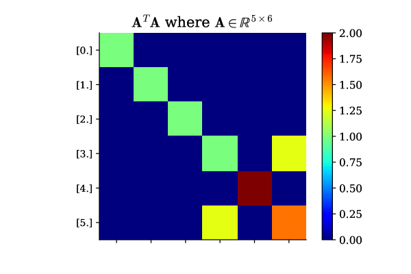
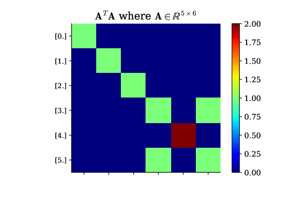
Figure 1: The Gram matrix $\bm{G}$ for three quadrature rules showing their practical degrees of exactness: (a) Gauss-Legendre; (b) Gauss-Lobatto; (c) Clenshaw-Curtis. The vertical axis in the figures show the polynomial degree and the colorbar shows the values of the entries of these matrices.

Classical extensions of Gauss quadrature include:

• Gauss-Radau and Gauss-Lobatto: The addition of end-points $(a,b)$ in quadrature rules. In Gauss-Radau the addition of one end-point $(a,b]=\left\{\zeta\in\rho|a<\zeta\leq b\right\}$ and both in Gauss-Lobatto, i.e., $[a,b]=\left\{\zeta\in\rho|a\leq\zeta\leq b\right\}$ gautschi1981survey .

• Gauss-Kronrod and Gauss-Patterson: Practical extensions of $m$-point Gauss rules by adaptively adding $m+1$ points to the quadrature rule to yield a combined degree of exactness of $(3m+1)$ or $(3n+2)$ depending on whether m is even or odd respectively; based on the work of Kronrod laurie1997calculation . Patterson patterson1968optimum rules are based on optimizing the degree of exactness of Kronrod points and with extensions to Lobatto rules. The intent behind these rules is that they admit certain favorable nesting properties.

• Gauss-Turán: The addition of derivative values (in conjunction with function values) within the integrand (see gautschi2004orthogonal ).

1.2 Multivariate extensions of classical rules

Multivariate extensions of univariate quadrature rules exist in the form of tensor product grids, assuming one is ready to evaluate a function at $m^{d}$ points. They are expressed as:

$$\begin{split}\int_{\mathbb{R}^{d}}f\left(\bm{\zeta}\right)\rho\left(\bm{\zeta}\right)d\bm{\zeta}&\approx\left(\mathcal{Q}_{q}^{m_{1}}\otimes\ldots\otimes\mathcal{Q}_{q}^{m_{d}}\right)\left(f\right)\\ &=\sum_{j_{1}=1}^{m_{1}}\ldots\sum_{j_{d}=1}^{m_{d}}f\left(\zeta_{j_{d}},\ldots,\zeta_{j_{d}}\right)\omega_{j_{1}}\ldots\omega_{j_{d}}\\ &=\sum_{j=1}^{m}f\left(\bm{\zeta}_{j}\right)\omega_{j}.\end{split}$$ (6)

The notation $\mathcal{Q}_{q}^{m_{i}}$ denotes a linear operation of the univariate quadrature rule applied to $f$ along direction $i$; the subscript $q$ stands for quadrature.

In the broader context of approximation, one is often interested in the projection of $f$ onto $\psi_{\bm{p}}\left(\bm{\zeta}\right)$. This pseudospectral approximation is given by

$$f\left(\bm{\zeta}\right)\approx\sum_{i=1}^{n}x_{i}\bm{\psi_{i}}\left(\bm{\zeta}\right), x_{i}=\sum_{j=1}^{m}f\left(\bm{\zeta}_{j}\right)\bm{\psi}_{i}\left(\bm{\zeta}_{j}\right)\omega_{j}.$$ where (7)

Inspecting the decay of these pseudospectral coefficients, i.e., $\mathbf{x}=\left(x_{1},\ldots,x_{m}\right)^{T}$ is useful for analyzing the quality of the overall approximation to $f\left(\bm{\zeta}\right)$, but more specifically for gaining insight into which directions the function varies the greatest, and to what extent. We remark here that for simulation-based problems where an approximation to $f\left(\bm{\zeta}\right)$ may be required, it may be unfeasible to evaluate a model at a tensor grid of quadrature points, particularly if $d$ is large. Sparse grids gerstner1998numerical ; smolyak1963quadrature offer moderate computational attenuation to this problem. One can think of a sparse grid as linear combinations of select anisotropic tensor grids

$$\int_{\mathbb{R}^{d}}f\left(\bm{\zeta}\right)\rho\left(\bm{\zeta}\right)d\bm{\zeta}\approx\sum_{\bm{r}\in\mathcal{K}}\bm{\alpha}\left(\bm{r}\right)\left(\mathcal{Q}_{q}^{m_{1}}\otimes\ldots\otimes\mathcal{Q}_{q}^{m_{d}}\right)\left(f\right),$$ (8)

where for a given level $l$—a variable that controls the density of points and the highest order of the polynomial in each direction—the multi-index $\mathcal{K}$ and coefficients $\bm{\alpha}(\bm{r})$ are given by

$$\mathcal{K}=\left\{\bm{r}\in\mathbb{N}^{d}:l+1\leq\left|\bm{r}\right|\leq l+d\right\}\;\;\text{and}\;\;\bm{\alpha}\left(\bm{r}\right)=\left(-1\right)^{-\left|\bm{r}\right|+d+l}\binom{d-1}{-\left|\bm{r}\right|+d+l}.$$ (9)

Formulas for the pseudospectral approximations via sparse grid integration can then be written down; we omit these in this exposition for brevity.

Approximation via sparse grids: To motivate the use of sparse grids, and to realize its limitations, consider the bi-variate function

$$f\left(\bm{\zeta}\right)=exp\left(3\zeta_{1}+\zeta_{2}\right)\;\;\;\text{where}\;\;\;\bm{\zeta}\in\left[-1,1\right]^{2}$$ (10)

and $\rho(\bm{\zeta})$ is the uniform distribution over the domain. Figure 2(a) plots the points in the parameter space for an isotropic tensor product grid using tensor products of order 35 Gauss-Legendre quadrature points, while (b) plots estimates of the pseudospectral coefficients using a tensor product Legendre polynomial basis in $\bm{\psi}_{\bm{p}}$. A total of 1296 function evaluations were required for these results.

Upon inspecting (b) it is apparent that coefficients with a total order of 12 and greater can be set to zero with near negligible change in the function approximation. In Figure 2(c, d) and (e, f) we present two solutions that achieve this. Figure 2(c-d) plot the results for a sparse grid with a linear growth rule (essentially emulating a total order index set) with $l=12$, requring 1015 function evaluations, while in Figure 2(e-f) the results show an exponential growth rule with $l=5$, requiring 667 function evaluations. Clearly, using sparse grid quadrature rules can reduce the number of model evaluations compare to tensor product grids.

2

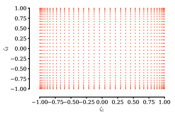
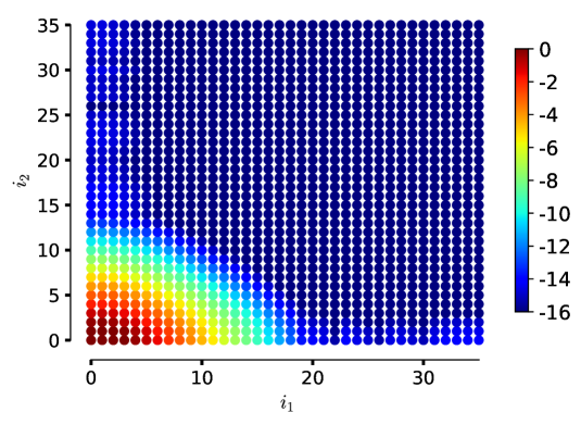
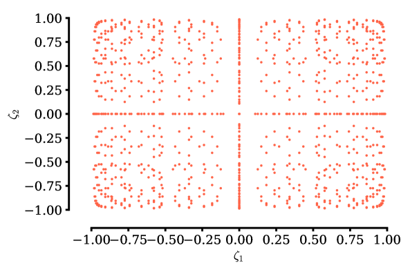
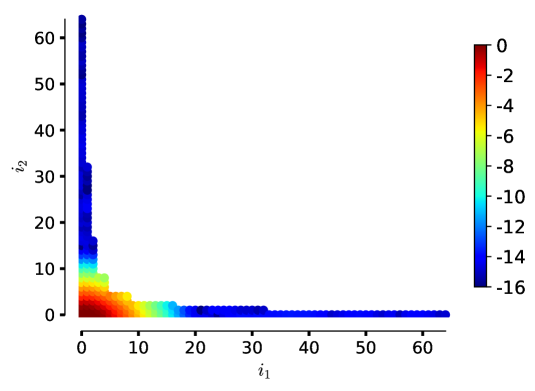
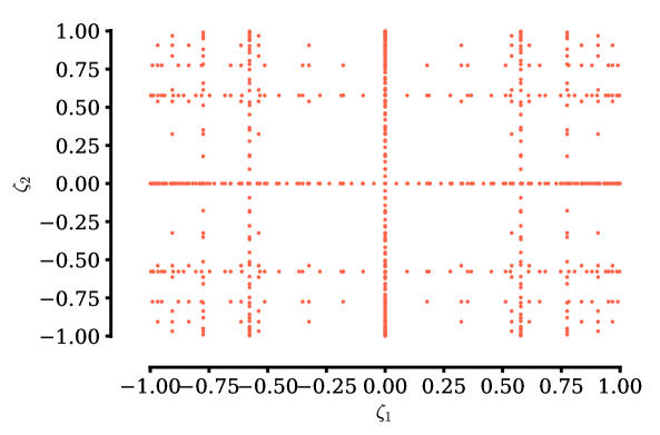
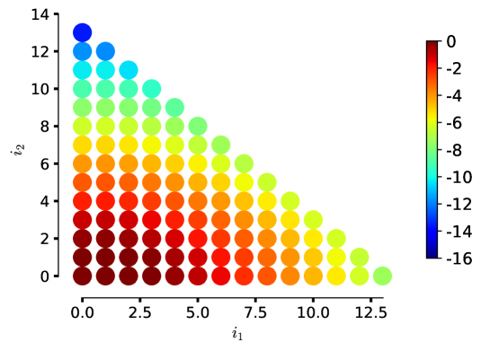
Figure 2: Parameter space points and pseudospectral coefficients (shown on a log base 10 scale) obtained via a (a, b) tensor grid with a maximum univariate order of 35; (c, d) sparse grid with a linear growth rule and $l=12$; (e, f) sparse grid with an exponential growth rule and $l=6$. The number of unique quadrature points from the three experiments were 1296, 1015 and 667 respectively.

While sparse grids and their adaptive variants conrad2013adaptive ; pfluger2010spatially are more computationally tractable than tensor product grids, they are still restricted to very specific index sets, even with linear, exponential and slow exponential burkardt2014slow growth rules. Furthermore, when simulation-based function evaluations at the quadrature points fail (or are corrupted), one may have to resort to interpolation heuristics. In comparison, least squares methods offer far more flexibility—both in terms of a choice of the basis and in negotiating failed simulations.

1.3 Scope and outline of paper

Our specific goal in this paper is to use ideas from polynomial least squares to generate quadrature rules. Without loss of generality, these quadrature rules will be used to estimate the pseudospectral coefficients $\mathbf{x}$ by solving

$$\underset{\mathbf{x}\in\mathbb{R}^{n}}{\text{minimize}}\;\;\;\left\|\bm{A}\mathbf{x}-\mathbf{b}\right\|_{2},$$ (11)

where we define the elements of $\bm{A}\in\mathbb{R}^{m\times n}$ as per (4). For completeness, we restate this definition but now in the multivariate setting, i.e.,

$$\bm{A}(i,\bm{j})=\bm{\psi}_{\bm{j}}\left(\bm{\zeta}\right)\sqrt{\omega_{i}},\;\;\;\;\;\bm{j}\in\mathcal{I},\;\;\;\text{card}\left(\mathcal{I}\right)=n,\;\;\;i=1,\ldots,m.$$ (12)

Typically $\mathcal{I}$ will be either a total order or a hyperbolic basis. The entries of the vector $\mathbf{b}\in\mathbb{R}^{m}$ comprise of weighted model evaluations at the $m$ quadrature points; individual entries are given by $\mathbf{b}(i)=\sqrt{\omega}_{i}f\left(\bm{\zeta}_{i}\right)$. Assuming $\bm{A}$ and $\mathbf{b}$ are known, solving (11) is trivial—the standard QR factorization can be used. However, the true challenge lies in selecting multivariate quadrature points and weights $\left\{\left(\bm{\zeta}_{i},\omega_{i}\right)\right\}_{i=1}^{m}$, such that:

• For a given choice of $n$, the number of quadrature points $m$ can be minimized and yield a rule that has a high degree of exactness;

• The least squares approximation in (11) is accurate;

• The least squares solution is stable with respect to perturbations in $\mathbf{b}$.

We will explore different strategies for generating $\bm{A}$ and techniques for subsampling it—even introducing a new approach in secti.on 3.2. Broadly speaking, strategies for computing multivariate quadrature points and weights via least squares involve two key decisions:

1. Selecting a sampling strategy: A suitable discretization of the domain from which quadrature points need to be computed;

2. Formulating an optimization problem: The strategy for subselecting points from this sampling (if required) via the optimization of a suitable objective.

Our goal in this manuscript is to describe the various techniques for generating these quadrature points and to make precise statements (where permissible) on their computational complexity. We substantiate our detailed review of literature with examples using the open-source code Effective Quadratures seshadri2017effective .

2 Selecting a sampling strategy

In this section we present methods for discretizing the domain based on the support of the parameters and their distributions. The survey builds on a recent review of sampling techniques for polynomial least squares hadigol2017least and from more recent texts including Narayan narayan2017computation ; narayan2017christoffel and Jakeman and Narayan jakeman2017generation .

Intuitively, the simplest sampling strategy for polynomial least squares is to generate random Monte-Carlo type samples based on the joint density $\rho(\bm{\zeta})$. Migliorati et al. migliorati2014analysis provide a practical sampling heuristic for obtaining well conditioned matrices $\bm{A}\in\mathbb{R}^{m\times n}$; they suggest sampling with $m=n^{2}$ for total degree and hyperbolic cross spaces. Furthermore, they prove that as the number of samples $m\rightarrow\infty$, the condition number $\kappa\left(\bm{A}^{T}\bm{A}\right)\rightarrow 1$ (see page 441 in migliorati2014analysis ). While these random samples can be pruned down using the optimization strategies presented in 3, there are other sampling alternatives.

2.1 Christoffel samples

The Christoffel sampling recipe of Narayan and co-authors narayan2017christoffel significantly outperforms the Monte Carlo approach in most problems. To understand their strategy, it will be useful to define the diagonal of the orthogonal projection kernel

$$K_{n}\left(\bm{\zeta}\right)\coloneqq\sum_{j=1}^{n}\bm{\psi}_{\bm{j}}^{2}\left(\bm{\zeta}\right),$$ (13)

where as before the subscript $n$ denotes $\text{card}\left(\mathcal{I}\right)$. We associate the above term with a constant

$$\left\|K\right\|_{\infty}\triangleq\underset{\bm{\zeta}\in\mathbb{R}^{D}}{sup}\left(K_{n}\left(\bm{\zeta}\right)\right),$$ (14)

which has a lower bound of $n$. Cohen et al. cohen2013stability prove that if the number of samples $m$ satisfies the bound

$$\frac{m}{nlog\left(m\right)}\apprge\chi\frac{\left\|K\right\|_{\infty}}{n},$$ (15)

for some constant $\chi$, then the subsequent least squares problem is both stable and accurate with high probability. The key ingredient to this bound, the quantity $\left\|K\right\|_{\infty}$, tends to be rather small for Chebyshev polynomials—scaling linearly with $n$ in the univariate case—but will be large for other polynomials, such as Legendre polynomials—scaling quadratically with $n$. Multivariate examples are given in chkifa2015discrete and lead to computationally demanding restrictions on the number of samples required to satisfy (15) narayan2017christoffel ; cohen2017optimal . Working with this bound, Narayan et al. provide a sampling strategy that leverages the fact that the asymptotic characteristics for total order polynomials can be determined. Thus, if the domain is bounded with a continuous $\rho$, then limit of $m/K_{n}$—known as the Christoffel function—is given by

$$\underset{n\rightarrow\infty}{\text{lim}}\;\frac{m}{K_{n}\left(\bm{\zeta}\right)}=\frac{\bm{\rho}\left(\bm{\zeta}\right)}{\nu\left(\bm{\zeta}\right)}$$ (16)

where the above statements holds weakly, and where $\nu(\bm{\zeta})$ is the weighted pluripotential equlibrium measure (see section 2.3 in narayan2017christoffel for the definition and significance). This implies that the functions $\bm{\phi}=\bm{\psi}\sqrt{m/K_{n}}$ form an orthogonal basis with respect to a modified weight function $\bm{\rho}K_{n}/m$. This in turn yields a modified reproducing diagonal kernel

$$\hat{K}_{n}=\sum_{j=1}^{m}\bm{\phi}^{2}=\frac{n}{K_{n}}K_{n}=n,$$ (17)

which attains the optimal value of $n$. The essence of the sampling strategy is to sample from $\nu$ (performing a Monte Carlo on the basis $\bm{\phi}$), which should in theory reduce the sample count as dictated by (15).

The challenge however is devleoping computational algorithms for generating samples according to $\nu(\bm{\zeta})$, since precise analytical forms are only known for a few domains. For instance, when $D=[-1,1]^{d}$, the measure $\nu(\bm{\zeta})$ is the Chebyshev (arcsine) distribution. Formulations for other distributions such as the Gaussian and exponential distributions are in general more complex and can be found in section 6 of narayan2017christoffel .

Comparing condition numbers: But how much lower are the condition numbers when we compare standard Monte Carlo with Christoffel sampling? Figure 3 plots the mean condition numbers (averaged over 10 trials) for Legendre polynomials in $d=2$ in (a) and (b), and $d=4$ in (c) and (d). Two different oversampling factors are also applied; (a) and (c) have an oversampling factor of $1.2$ while (b) and (d) have an oversampling factor of $2$–i.e., $m=2n$. For the Christoffel results, the samples are generated from the Chebyshev distribution.

It is apparent from these figures that the Christoffel sampling strategy does produce more well conditioned matrices on average. We make two additional remarks here. The first concerns the choice of the weights. In both sampling strategies the quadrature weights $\omega_{i}$ are computed via

$$\omega_{i}=\frac{\tilde{\omega}_{i}}{\sum_{k=1}^{m}\tilde{\omega}_{k}},\;\;\;\text{where}\;\;\;\tilde{\omega}_{i}=\frac{n}{m}\sum_{\bm{j}\in\mathcal{I}}\bm{\psi}_{\bm{j}}^{2}\left(\bm{\zeta}_{i}\right)$$ (18)

ensuring that the weights sum up to unity. The second concerns the Gram matrix $\bm{A}^{T}\bm{A}$, shown in Figure 4 for the Christoffel case with a maximum order of 3, with $d=4$ and an oversampling factor of $2$. Although the condition number of this matrix is very low (4.826), one can clearly observe sufficient internal aliasing errors that would likely effect subsequent numerical computation of moments.

2

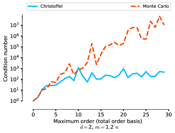
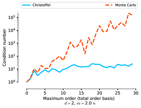
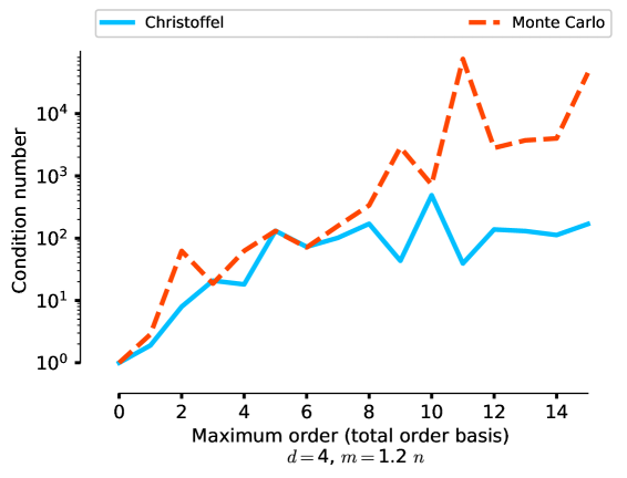
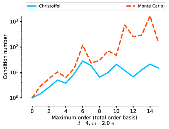
Figure 3: A comparison of condition numbers for $\bm{A}$ when constructing the matrix using multivariate Legendre polynomials evaluated at either Monte Carlo or Christoffel samples. Experiments for (a) $d=2,m=1.2n$; (b) $d=2,m=2n$; (c) $d=4,m=1.2n$; (d) $d=2,m=2n$. Plotted are the mean values of 10 random trials.

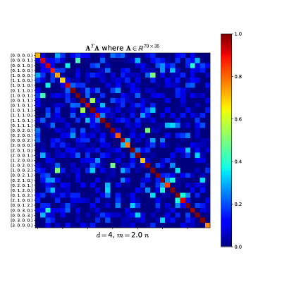
Figure 4: The Gram matrix $\bm{G}=\bm{A}^{T}\bm{A}$ for one of the trials for the case where $d=4$ and $m=2n$ showing its deviation from the identity.

2.2 Subsampling tensor grids

The idea of constructing $\bm{A}$ using samples from a tensor grid and then subsampling its rows has been explored from both compressed sensing tang2014subsampled and least squares zhou2015weighted ; seshadri2017effectively perspectives. In Zhou et al. zhou2015weighted the authors randomly subsample the rows and demonstrate stability in the least squares problem with $m$ scaling linearly with $n$. In Seshadri et al., seshadri2017effectively , a greedy optimization strategy is used to determine which subsamples to select; they report small condition numbers even when $n=m$ for problems where $d\leq 7$ and a total order of degree $\leq 15$. Details of their optimization strategy are presented in section 3. One drawback of their technique is the requirement that the full $\bm{A}$ matrix must be stored and passed onto the optimizer—a requirement that can be circumvented in the randomized approach, albeit at the cost of $m$ being greater than $n$ (typically). A representative comparison of the condition numbers is shown in Figure 5. In these results, the isotropic tensor grid from which the subsamples are computed corresponds to the highest total order of the polynomial basis (shown on the horizontal axis).

2

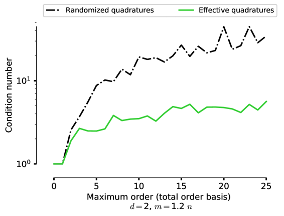
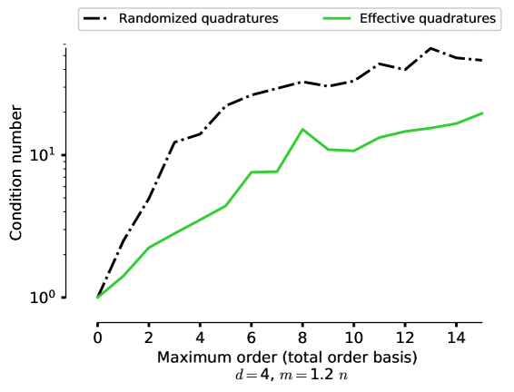
Figure 5: A comparison of condition numbers for $\bm{A}$ when constructing the matrix using multivariate Legendre polynomials evaluated at either randomized or effectively subsampled quadrature points. Experiments for (a) $d=2,m=1.2n$; (b) $d=4,m=1.2n$. For the randomized technique, we plot the mean values of 10 random trials.

2.3 Coherence and induced sampling

Building on some of the ideas discussed previously in 2.1, one can detail an importance sampling strategy that yields stable least squares estimates for $m\apprge n$, up to log factors. The essence of the idea is to define a new distribution $\mu$ such that

$$\mu=\frac{K_{n}}{n}\bm{\rho}=\frac{1}{n}\left(\sum_{j=1}^{n}\bm{\psi}_{j}^{2}\left(\bm{\zeta}\right)\right)\bm{\rho}.$$ (19)

It should be noted that while $\bm{\rho}$ is a product measure and therefore easy to sample from, $\mu$ is not and thus requires either techniques based on Markov chain Monte Carlo (MCMC) or conditional sampling cohen2017optimal . More specifically, $\mu$ depends on $m$, so if one enriches the space with more samples or change the basis, then $\mu$ will change. In hampton2015coherence , the authors devise an MCMC strategy which seeks to find $\mu$, thereby explicitly minimizing their coherence parameter (a weighted form of $\left\|K\right\|_{\infty}$ ). In narayan2017computation , formulations for computing $\mu$ via induced distributions is detailed. In our numerical experiments investigating the condition numbers of matrices obtained via such induced samples—in a similar vein to the Figures 3—the condition numbers were found to be comparable to those from Christoffel sampling.

3 Optimization strategies

In the case of Christoffel, Monte Carlo and even subsampling based techniques, a reduction in $m$ can be achieved, facilitating near quadrature like degree of exactness properties. In this section we discuss various optimization techniques for achieving this.

3.1 Greedy linear algebra approaches

It will be convenient to interpret our objective as identifying a suitable submatrix of $\bm{A}\in\mathbb{R}^{m\times n}$ by only selecting $k<<m$ rows. Ideally, we would like $k$ to be as close to $n$ as possible. Formally, we write this submatrix as

$$\begin{split}\hat{\bm{A}}_{\mathbf{z}}&=\frac{1}{\tau}\sum_{i=1}^{m}z_{i}\mathbf{a}_{i}^{T}\mathbf{e}\\ \text{where}\;\;\;&\mathbf{1}^{T}\mathbf{z}=k,\\ &\tau=\sum_{i=1}^{m}z_{i}w_{i},\\ &z_{i}\in\left\{0,1\right\}\end{split}$$ (20)

and where $\mathbf{a}_{i}^{T}$ represents the rows of $\bm{A}$, and $\mathbf{e}\in\mathbb{R}^{k}$ and $\mathbf{1}\in\mathbb{R}^{m}$ are vector of ones. The notation above indicates that $\mathbf{z}\in\mathbb{R}^{m}$ is a boolean vector. The normalization factor $\tau$ is introduced to ensure the weights associated with the subselected quadrature rule sum up to one.

Table 1 highlights some of the various optimization objectives that may be pursued for finding $\mathbf{z}$ such that the resulting $\hat{\bm{A}}_{\mathbf{z}}$ yields accurate and stable least squares solutions.

Table 1: Sample objectives for optimization

Case	Objective
P1:	$\underset{\mathbf{z}}{\text{minimize}}\;\;\sigma_{max}\left(\hat{\bm{A}}_{\mathbf{z}}\right)$
P2:	$\underset{\mathbf{z}}{\text{maximize}}\;\;\sigma_{min}\left(\hat{\bm{A}}_{\mathbf{z}}\right)$
P3:	$\underset{\mathbf{z}}{\text{minimize}}\;\;\kappa\left(\hat{\bm{A}}_{\mathbf{z}}\right)$
P4:	$\underset{\mathbf{z}}{\text{maximize}}\;\;\text{vol}\left(\hat{\bm{A}}_{\mathbf{z}}\right)=\prod_{i=1}^{k}\sigma_{i}\left(\hat{\bm{A}}_{\mathbf{z}}\right)$
P5:	$\underset{\mathbf{z}}{\text{minimize}}\;\;\left\|\hat{\bm{A}}_{\mathbf{z}}^{T}\hat{\bm{A}}_{\mathbf{z}}\right\|_{2}$

We remark here that objectives P1 to P4 are proven NP-hard problems (see Theorem 4 in Civril and Magdon-Ismail ccivril2009selecting ); although it is readily apparent that all the objectives require evaluating $\binom{m}{k}$ possible choices—a computationally unwieldy task for large values of $m$ and $k$. Thus some regularization or relaxation is necessary for tractable optimization strategies.

We begin by focusing on P4. In the case where $k=n$, one can express the volume maximization objective as a determinant maximization problem. Points that in theory maximize this determinant, i.e., the Fekete points, yield a Lebesgue constant that typically grows logarithmically—at most linearly—in $n$ bos2006bivariate . So how do we find a determinant maximizing submatrix of $\bm{A}$ by selecting $k$ of its rows? In Guo et al. guo2018weighted the authors show that if there exists a point stencil that indeed maximizes the determinant, then a greedy optimization can recover the global optimum (see Theorem 3.2 in Guo et al.). Furthermore, the authors prove that either maximizing the determinant or minimizing the condition number (P3) is likely to yield equivalent solutions. This explains their use of the pivoted QR factorization for finding such points; its factorization is given by

$$\bm{A}^{T}\bm{P}=\bm{Q}\left(\begin{array}[]{cc}\bm{R}_{1}&\bm{R}_{2}\end{array}\right),$$ (21)

where $\bm{Q}\in\mathbb{R}^{n\times n}$ is an orthogonal matrix and $\bm{R}_{1}\in\mathbb{R}^{n\times n}$ is an upper triangular matrix that is invertible and $\mathbb{R}^{n\times(m-n)}$. The permutation matrix $\bm{P}\in\mathbb{R}^{m\times m}$ is based on a pivoting strategy that seeks to either maximize $\sigma_{max}(\bm{R}_{1})$ or minimize $\sigma_{min}(\bm{R}_{2})$. As Björck notes (see section 2.4.3 in bjorck2016numerical ) both these strategies are in some cases equivalent and thus greedily maximize the diagonal entries of $\bm{R}_{1}$ and therefore serve as heuristics for achieving all the objectives in Table 1. Comprehensive analysis on pivoted QR factorizations can be found in chandrasekaran1994rank ; chan1994low ; dax2000modified . Techniques for the closely related subset selection problem can also be adopted and build on ideas based on random matrix theory (see Deshpande and Rademacher deshpande2010efficient and references therein). The monograph by Miller miller2002subset which also provides a thorough survey of techniques, emphasizes the advantages of methods based on QR factorizations.

Optimizing to find Gauss points: In the univariate case, it is known that Gauss-Legendre quadrature points are optimal with respect to a uniform measure. In an effort to gauge the efficacy of some of the optimization strategies discussed in this paper, we carry out a simple numerical experiment. Let $\bm{A}\in\mathbb{R}^{101\times K}$ be formed by evaluating up to order $K$ Legendre polynomials at the first 101 Gauss-Legendre quadrature points. Each of the aforementioned greedy strategies is tasked with finding a suitable submatrix $\hat{\bm{A}}_{\mathbf{z}}\in\mathbb{R}^{K\times K}$. The quadrature points embedded in $\mathbf{z}$ for $K=4$ and $K=8$ are shown in Figure 6(a) and (b) respectively. It is interesting to observe how the points obtained from LU with row pivoting, QR with column pivoting and SVD-based subset selection all closely approximate the Gauss-Legendre points! This figure—and the numerous other cases we tested for $d=1$—show that the difference between the various optimization strategies is not incredibly significant; all of them tend to converge close to the optimal solution.

But what happens when $d$ increases? Figure 7(a) plots the subsampled points obtained from the three linear algebra optimization strategies when subsampling from a tensor grid with order 50 in both $\zeta_{1}$ and $\zeta_{2}$ directions. The basis used—i.e., the columns of $\bm{A}$—is an isotropic tensor product with an order of 3. As expected, the obtained points are very similar to Gauss-Legendre tensor product points with order 3. In Figure 7(b), instead of subsampling from a higher order tensor grid, we subsample from Christoffel samples, which in the uniform case corresponds to the Chebyshev distribution; the basis is the same as in (a). In this case it is interesting to note that the LU and QR pivoting approaches, which are similar, yield slightly different results when compared to the SVD approach.

2

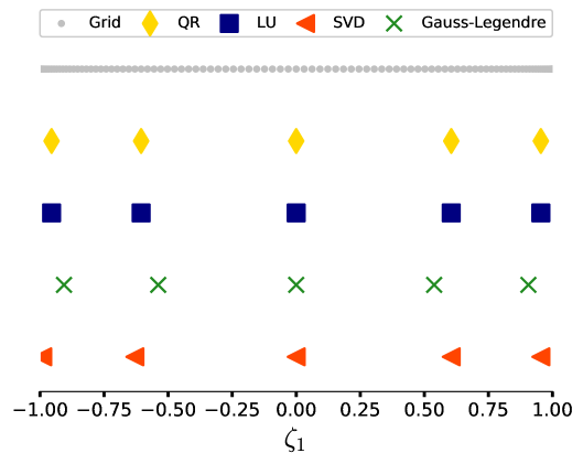
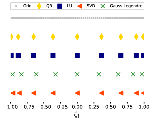
Figure 6: Approximation to the Gauss-Legendre quadrature points obtained by subsampling from a grid of order 100 using various optimization strategies with an (a) order 4; (b) order 8 Legendre polynomial basis.

2

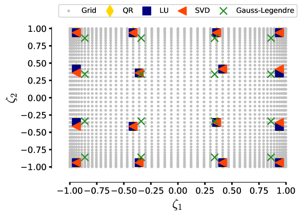
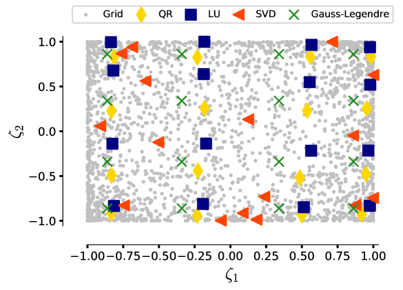
Figure 7: Approximation to the $[3,3]$ Gauss-Legendre quadrature points obtained by subsampling from a grid of with 2601 samples using various optimization strategies: (a) Subsampling from a tensor grid of order $[50,50]$; (b) Subsampling from 2601 randomly distributed Chebyshev points.

The use of such rank revealing factorizations for minimizing the condition number of a Vandermonde-type matrix have been previously investigated in bos2010computing ; seshadri2017effectively albeit on different meshes. When pruning rows from $\bm{A}$, the condition number of $\hat{\bm{A}}_{\mathbf{z}}$ can be bounded by

$$\kappa\left(\hat{\bm{A}}_{\mathbf{z}}\right)\leq\kappa\left(\bm{A}\right)\sqrt{1+s^{2}n\left(m-n\right)},$$ (22)

where $s>1$ is a constant based on the pivoting algorithm. In Seshadri et al. seshadri2017effectively the authors draw upon a subset selection strategy from Chapter 5 of golub2012matrix that uses both the SVD and a rank revealing QR factorization for identifying a more well conditioned submatrix. However, as $m$ and $n$ get progressively larger, the costs associated with computing both the SVD $\mathcal{O}(m^{2}n^{3})$ and a Householder (or modified Gram-Schmidt)-based rank revealing QR factorization should be monitored. Other rank revealing techniques such as strong LU factorizations miranian2003strong and randomized QR with column pivoting martinsson2017householder ; duersch2017randomized may also be opted for.

To speed up the optimization process—a consideration that may be ignored when model evaluations themselves take hours—other techniques have been proposed. Shin and Xiu shin2016nonadaptive ; shin2016near optimize a metric similar to P4

$$\underset{\mathbf{z}}{\text{maximize}}\left(\frac{\sqrt{\text{det}\left(\hat{\bm{A}}_{\mathbf{z}}^{T}\hat{\bm{A}}_{\mathbf{z}}\right)}}{\prod_{i=1}^{k}\left\|\hat{\bm{A}}_{\mathbf{z}}(i)\right\|}\right)^{1/k},$$ (23)

where $\hat{\bm{A}}(i)_{\mathbf{z}}$ denotes the $i-$th column of $\hat{\bm{A}}_{\mathbf{z}}$. To ascertain which rows $\mathbf{z}$ to use, the authors outline a greedy strategy that begins with a few initially selected rows and then adds rows based on whether they increase the determinant of the Gramian, $\hat{\bm{A}}_{\mathbf{z}}^{T}\hat{\bm{A}}_{\mathbf{z}}$. To abate the computational cost of computing the determinant for each candidate, they devise a rank-2 update to the determinant (of the Gramian) based on Sylvester’s determinant formula and the Sherman-Morrison formula. In a similar vein, Ghili and Iaccarino ghili2017least lay out a series of arguments—motivated by reducing the operational complexity of the determinant-based optimization—for optimizing the trace of the design matrix instead. They observe that since the Frobenius norm is an upper bound on the spectral norm and because all the singular values contribute to the aliasing error, optimizing over this norm will undoubtedly yield a small spectral norm. The authors formulate a coordinate descent optimization approach to find suitable points and weights.

3.2 Convex relaxation via Newton’s method

In general the aforementioned objectives are non-convex. We discuss an idea that permits these objectives to be recast as a convex optimization problem. Our idea originates from the sensor selection problem hovland1997dynamic ; kincaid2002d : given a collection of $m$ sensor measurements—where each measurement is a vector—select $k$ measurements such that the error covariance of the resulting ellipsoid is minimized. We remark here that while a generalized variant of the sensor selection problem is NP-hard (see bian2006utility ); the one we describe below has not yet been proven to be NP-hard. Furthermore, by selecting the optimization variable to be a boolean vector $\mathbf{z}$ that restricts the measurements selected, this problem can be cast as a determinant maximization problem vandenberghe1998determinant where the objective is a concave function in $\mathbf{z}$ with binary constraints on its entries. This problem can be solved via interior point methods and has complexity $\mathcal{O}(m^{3})$. Joshi and Boyd joshi2009sensor provide a formulation for a relaxed sensor selection problem that can be readily solved by Newton’s method, where the binary constraint can be substituted with a penalty term added to the objective function. By replacing their sensor measurements with rows from our Vandermonde type matrix, one arrives at the following maximum volume problem

$$\begin{split}\underset{\mathbf{z}\in\mathbb{R}^{M}}{\text{minimize}}\;\;\;&-\text{log}\;\text{det}\left(\frac{1}{\tau}\sum_{i=1}^{M}z_{i}\mathbf{a}_{i}^{T}\mathbf{e}\right)-\lambda\sum_{i=1}^{M}\left(\text{log}\left(z_{i}\right)+\text{log}\left(1-z_{i}\right)\right)\\ \text{subject to}\;\;\;&\mathbf{1}^{T}\mathbf{z}=K\\ &0\leq z_{i}\leq 1,\;i=1,\ldots,M.\end{split}$$ (24)

where the positive constant $\lambda$ is used to control the quality of the approximation. Newton’s approach has complexity $\mathcal{O}(m^{3})$ with the greatest cost arising from the Cholesky factorization when computing the inverse of the Hessian joshi2009sensor . The linear constraint is solved using standard KKT conditions as detailed in page 525 of boyd2004convex . In practice this algorithm requires roughly 10-20 iterations and yields surprisingly good results for finding suitable quadrature points.

Padua points via Convex optimization: It is difficult to select points suitable for interpolation with total order polynomials, that are unisolvent—a condition where the points guarantee a unique interpolant trefethen2017cubature . One such group of points that does admit unisolvency are the famous Padua points. For a positive integer $N$, these points are given by $(\zeta^{(1)}_{m},\zeta^{(2)}_{m})\in[-1,1]^{2}$ where

$$\zeta^{(1)}_{m}=cos\left(\frac{\pi\left(m-1\right)}{N}\right),\zeta^{(2)}_{m}=\begin{cases}\begin{array}[]{c}cos\left(\frac{\pi\left(2k-1\right)}{N-1}\right)\\ cos\left(\frac{\pi\left(2k-2\right)}{N-1}\right)\end{array}&\begin{array}[]{c}m\;\textrm{odd}\\ m\;\textrm{even}\end{array}\end{cases}$$ (25)

and $1\leq m\leq N+1$, $1\leq k\leq 1+N/2$ caliari2011padua2dm . The Padua points have a provably minimal growth rate of $\mathcal{O}(log^{2}N)$ of the Lebesgue constant, far lower than Morrow-Patterson or the Extended Morrow-Patterson points bos2006bivariateb . Two other characterizations may also be used to determine these points; they are formed by the intersection of certain Lissajous curves and the boundary of $[-1,1]^{2}$ or alternatively, every other point from an $(N+1)\times(N+2)$ tensor product Chebyshev grid bos2006bivariate ; bos2007bivariate .

As an example, consider the case where $N=4$ resulting in a 30-point Chebyshev tensor grid and a total order basis where the highest order is 4. Figure 8(a) plots the corresponding gram matrix $\bm{G}=\bm{A}^{T}\bm{A}$. As expected the quadrature rule can integrate all polynomials except for the one corresponding to the last row, i.e., $\bm{\psi_{(4,0)}}$, whose integrand has an order of 8 along the first direction $\zeta_{1}$, beyond the degree of exactness of the 5 points. What is fascinating is that when these points are subsampled one can get a subsampled Gram matrix i.e., $\hat{\bm{A}}_{\mathbf{z}}^{T}\hat{\bm{A}}_{\mathbf{z}}$ to have the same degree of exactness, as illustrated in Figure 8(b). To obtain this result, the aforementioned convex optimization via Newton’s method was used on $\bm{A}$, yielding the Padua points—i.e., every alternate point from the 30-point Chebyshev tensor grid.

2

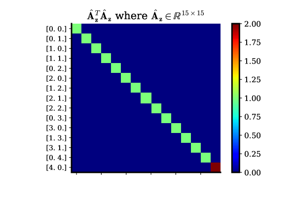
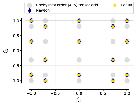
Figure 8: The Gram matrix associated with Chebyshev tensor product grid with $4\times 5=30$ points and a total order basis with maximum degree of 4 in (a). The subsampled Gram matrix via convex optimization in (b) and a comparison of the samples and subsamples in (c).

Comparing execution time: In our numerical experiments on some of the aforementioned optimization strategies, we have alluded to the operational complexity. We make an obvious remark here, that as the both the polynomial degree and the dimension increases, the computing time rises. Non-linear algebra approaches such as ghili2017least and the Newton approach presented here, have other tunable parameters that can either add to, or decrease computational run time.

Figure 9 plots the running times for $d=3$ and $m=n$ when subsampling from grid of Chebyshev points—where the number of points is given by the $\left(\text{maximum total order}+1\right)^{d}$—using the different optimization strategies. These experiments were carried out on a 3.1 GHz i7 Macbook Pro with 16GB of RAM. For completeness, a summary of the operational complexity of these techniques is provided in 2. The condition numbers of the matrices obtained from QR, LU and the SVD approach were generally lower (similar order of magnitude) than those obtained from the other two techniques.

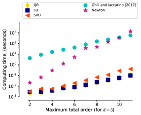
Figure 9: Representative computing times for the different optimization strategies for $m=n$ and $d=3$ using Chebyshev samples and a total order basis.

Table 2: Summary of the operational complexity of some of the optimization strategies.

Optimization strategy	Complexity
SVD-based subset selection	$\mathcal{O}\left(nm^{2}\right)+\mathcal{O}\left(nm^{2}\right)$
QR column pivoting	$\mathcal{O}\left(nm^{2}\right)$
LU row pivoting	$\mathcal{O}\left(m^{2}\right)$
Newton’s method	$\mathcal{O}\left(n^{3}\right)$
Frobenius norm optimization (Ghili and Iaccarino 2017)	$\mathcal{O}\left(dnm^{2}\right)$

3.3 Moment-based optimization strategies

To motivate this section, consider the integration property of orthogonal polynomials, highlighted in (5). In the univariate case, one can write

$$\begin{split}&\bm{P}\mathbf{w}=\mathbf{e}\\ \text{where}\;\;\;&\bm{P}(i,j)=\psi_{i}\left(\zeta_{j}\right),\;\;\;\mathbf{w}(i)=\omega_{i},\;\;\;\text{and}\;\;\;\mathbf{e}^{T}=\left[1,0,\ldots,0\right].\end{split}$$ (26)

Assuming $\bm{P}\in\mathbb{R}^{m\times m}$ where one uses the first m Gauss-Legendre points in $\zeta_{j}$ and the first $(m-1)$ order Legendre polynomials in $\psi_{i}$, then the solution $\mathbf{w}$ for the above linear set of equations will yield the first $m$ Gauss-Legendre weights. In the case where the points are not from a known quadrature rule—i.e., if they are from a random distribution—then one has to ensure that the weights are positive via a constraint.

Instead of working with matrices and optimizing for the objectives in Table 1, one can frame an optimization problem centered on the computation of moments where one optimizes over the space of quadrature weights (non-negative). This moment-based approach for finding quadrature points and weights is utilized in Keshavarzzadeh et al. keshavarzzadeh2018numerical where the authors solve a relaxed version of this constraint linear system by minimizing $\left\|\mathbf{P}\mathbf{w}-\mathbf{e}\right\|_{2}$. In Ryu and Boyd ryu2015extensions , the authors present numerical quadrature as a solution to the infinite-dimensional linear program

$$\begin{split}\underset{\mathbf{v}\in\mathbb{R}^{m}}{\text{minimize}}\;\;\;&\mathbf{f}^{T}\mathbf{v}\\ \text{subject to}\;\;\;&\mathbf{p}_{j}^{T}\mathbf{v}=c_{i},\;\;\;\text{where}\;\;\;i=1,\ldots,n.\end{split}$$ (27)

Here components of $\mathbf{f}\in\mathbb{R}^{m}$ are given by $\mathbf{f}\left(i\right)=f\left(\bm{\zeta}_{i}\right)$, and $\mathbf{p}_{j}\in\mathbb{R}^{m}$ has components $\mathbf{p}_{j}\left(i\right)=\bm{\psi}_{j}\left(\bm{\zeta}_{i}\right)$; the optimization variable $\mathbf{v}\left(i\right)=\omega_{i}$ represents the quadrature weights. The constants $c_{i}$ in the equality constraints are determined analytically, as they involve integrating a known polynomial over the support of $f$. The problem can be interpreted as a weighted $l_{1}$ optimization problem, as we require $\mathbf{v}$ to have as many zeros as possible and yet satisfy the above constraints. As this problem is NP-hard, Ryu and Boyd propose a two-stage approach to solve it; one for generating an initial condition and another for optimizing over $\mathbf{v}$. Their approach has been recently adapted in Jakeman and Narayan jakeman2017generation who propose least absolute shrinkage and selection operator (LASSO) for finding the initial condition. They then proceed to solve the optimization using a gradient-based nonlinear least squares optimizer. Their results are extremely promising—numerical experiments using their technique show orders of magnitude improvement in convergence compared to tensor and sparse grid rules.

4 Concluding remarks and the future

In this paper, we provided an overview of strategies for finding quadrature points using ideas from polynomial least squares. Although we have sought to keep our review as detailed as possible, readers will forgive us for omitting various techniques. For example, we did not discuss optimal design of experiment based samples, although we point the interested reader to the review offered in hadigol2017least ; for convex relaxations of the various optimal design of experiment problems we refer the reader to section 7.5.2 of Boyd and Vandenberghe boyd2004convex . In addition, we have also highlighted a new convex optimization strategy that uses Newton’s method for finding the best subsamples by maximizing the volume of the confidence ellipsoid associated with the Vandermonde-type matrix.

So what’s next? Based on our review we offer a glimpse of potential future areas of research that could prove to be fruitful:

1. Randomized greedy linear algebra approaches for finding suitable quadrature samples. Existing approaches are tailored for finding pivot columns for tall matrices; for our problem we require these techniques to be applicable to fat matrices.

2. Large scale (and distributed) variants of the convex optimization strategies detailed, including an alternating direction method of multiplies (ADMM) boyd2011distributed formulation for the Newton’s method technique presented in this paper;

3. Heuristics for optimizing the weights when the joint density of the samples is not known—a problem that arises in data science; typically in uncertainty quantification the joint density $\bm{\rho}$ is assumed to be known.

4. The development of an open-source repository of near-optimal points for the case where $m=n$ for different total order basis and across different $d$.

5. Building on (1) and following the recent work by Shin and Xiu shin2017randomized and Wu et al. wu2017randomized , the use of approaches such as the randomized Kaczmarz algorithm strohmer2009randomized for solving the least squares problem in (11). The essence of the idea here is that as $d$ and the highest multivariate polynomial degree get larger, the matrix $\hat{\mathbf{A}}_{\mathbf{z}}$ can not be stored in memory—a requirement for standard linear algebra approaches. Thus techniques such as the Kaczmarz algorithm, which solve for $\mathbf{x}$ by iteratively requiring access to rows of $\hat{\mathbf{A}}_{\mathbf{z}}$ and elements of $\mathbf{b}$, are useful.

References

- (1) Ben Adcock and Daan Huybrechs. Approximating smooth, multivariate functions on irregular domains. arXiv preprint arXiv:1802.00602, 2018.
- (2) Fang Bian, David Kempe, and Ramesh Govindan. Utility based sensor selection. In Proceedings of the 5th international conference on Information processing in sensor networks, pages 11–18. ACM, 2006.
- (3) Åke Björck. Numerical methods in matrix computations. Springer.
- (4) Géraud Blatman and Bruno Sudret. Adaptive sparse polynomial chaos expansion based on least angle regression. Journal of Computational Physics, 230(6):2345–2367, 2011.
- (5) Len Bos, Marco Caliari, Stefano De Marchi, and Marco Vianello. Bivariate interpolation at xu points: results, extensions and applications. Electron. Trans. Numer. Anal, 25:1–16, 2006.
- (6) Len Bos, Marco Caliari, Stefano De Marchi, Marco Vianello, and Yuan Xu. Bivariate lagrange interpolation at the padua points: the generating curve approach. Journal of Approximation Theory, 143(1):15–25, 2006.
- (7) Len Bos, Stefano De Marchi, Alvise Sommariva, and Marco Vianello. Computing multivariate fekete and leja points by numerical linear algebra. SIAM Journal on Numerical Analysis, 48(5):1984–1999, 2010.
- (8) Len Bos, Stefano De Marchi, Marco Vianello, and Yuan Xu. Bivariate lagrange interpolation at the padua points: the ideal theory approach. Numerische Mathematik, 108(1):43–57, 2007.
- (9) Stephen Boyd, Neal Parikh, Eric Chu, Borja Peleato, Jonathan Eckstein, et al. Distributed optimization and statistical learning via the alternating direction method of multipliers. Foundations and Trends® in Machine learning, 3(1):1–122, 2011.
- (10) Stephen Boyd and Lieven Vandenberghe. Convex optimization. Cambridge university press, 2004.
- (11) John Burkardt. Slow exponential growth for clenshaw curtis sparse grids, 2014.
- (12) Marco Caliari, Stefano De Marchi, Alvise Sommariva, and Marco Vianello. Padua2dm: fast interpolation and cubature at the padua points in matlab/octave. Numerical Algorithms, 56(1):45–60, 2011.
- (13) Tony F Chan and Per Christian Hansen. Low-rank revealing qr factorizations. Numerical Linear Algebra with Applications, 1(1):33–44, 1994.
- (14) Shivkumar Chandrasekaran and Ilse CF Ipsen. On rank-revealing factorisations. SIAM Journal on Matrix Analysis and Applications, 15(2):592–622, 1994.
- (15) Abdellah Chkifa, Albert Cohen, Giovanni Migliorati, Fabio Nobile, and Raul Tempone. Discrete least squares polynomial approximation with random evaluations - application to parametric and stochastic elliptic pdes. ESAIM: Mathematical Modelling and Numerical Analysis, 49(3):815–837, 2015.
- (16) Ali Çivril and Malik Magdon-Ismail. On selecting a maximum volume sub-matrix of a matrix and related problems. Theoretical Computer Science, 410(47-49):4801–4811, 2009.
- (17) Albert Cohen, Mark A Davenport, and Dany Leviatan. On the stability and accuracy of least squares approximations. Foundations of computational mathematics, 13(5):819–834, 2013.
- (18) Albert Cohen and Giovanni Migliorati. Optimal weighted least-squares methods. SMAI Journal of Computational Mathematics, 3:181–203, 2017.
- (19) Patrick R Conrad and Youssef M Marzouk. Adaptive smolyak pseudospectral approximations. SIAM Journal on Scientific Computing, 35(6):A2643–A2670, 2013.
- (20) Philip J Davis and Philip Rabinowitz. Methods of numerical integration. Courier Corporation, 2007.
- (21) Achiya Dax. A modified gram–schmidt algorithm with iterative orthogonalization and column pivoting. Linear algebra and its applications, 310(1-3):25–42, 2000.
- (22) Amit Deshpande and Luis Rademacher. Efficient volume sampling for row/column subset selection. In Foundations of Computer Science (FOCS), 2010 51st Annual IEEE Symposium on, pages 329–338. IEEE, 2010.
- (23) Jed A Duersch and Ming Gu. Randomized qr with column pivoting. SIAM Journal on Scientific Computing, 39(4):C263–C291, 2017.
- (24) Walter Gautschi. A survey of gauss-christoffel quadrature formulae. In EB Christoffel, pages 72–147. Springer, 1981.
- (25) Walter Gautschi. Orthogonal polynomials—constructive theory and applications. Journal of Computational and Applied Mathematics, 12:61–76, 1985.
- (26) Walter Gautschi. Orthogonal polynomials: computation and approximation. Oxford University Press on Demand, 2004.
- (27) W Morven Gentleman. Implementing clenshaw-curtis quadrature, i methodology and experience. Communications of the ACM, 15(5):337–342, 1972.
- (28) Thomas Gerstner and Michael Griebel. Numerical integration using sparse grids. Numerical algorithms, 18(3):209–232, 1998.
- (29) Saman Ghili and Gianluca Iaccarino. Least squares approximation of polynomial chaos expansions with optimized grid points. SIAM Journal on Scientific Computing, 39(5):A1991–A2019, 2017.
- (30) Shahpar S. Ghisu, T. Toward affordable uncertainty quantification for industrial problems: Part ii turbomachinery application. ASME Turbo Expo 2017, GT2017-64845, 2017.
- (31) Gene H Golub and Charles F Van Loan. Matrix computations, volume 4. JHU Press, 2012.
- (32) Gene H Golub and John H Welsch. Calculation of gauss quadrature rules. Mathematics of computation, 23(106):221–230, 1969.
- (33) Ling Guo, Akil Narayan, Liang Yan, and Tao Zhou. Weighted approximate fekete points: Sampling for least-squares polynomial approximation. SIAM Journal on Scientific Computing, 40(1):A366–A387, 2018.
- (34) Mohammad Hadigol and Alireza Doostan. Least squares polynomial chaos expansion: A review of sampling strategies. Computer Methods in Applied Mechanics and Engineering, 2017.
- (35) Jerrad Hampton and Alireza Doostan. Coherence motivated sampling and convergence analysis of least squares polynomial chaos regression. Computer Methods in Applied Mechanics and Engineering, 290:73–97, 2015.
- (36) Geir E Hovland and Brenan J McCarragher. Dynamic sensor selection for robotic systems. In Robotics and Automation, 1997. Proceedings., 1997 IEEE International Conference on, volume 1, pages 272–277. IEEE, 1997.
- (37) John D Jakeman and Akil Narayan. Generation and application of multivariate polynomial quadrature rules. arXiv preprint arXiv:1711.00506, 2017.
- (38) Siddharth Joshi and Stephen Boyd. Sensor selection via convex optimization. IEEE Transactions on Signal Processing, 57(2):451–462, 2009.
- (39) T. S. Kalra, A. Aretxabaleta, P. Seshadri, N. K. Ganju, and A. Beudin. Sensitivity analysis of a coupled hydrodynamic-vegetation model using the effectively subsampled quadratures method. Geoscientific Model Development Discussions, 2017:1–28, 2017.
- (40) Vahid Keshavarzzadeh, Robert M Kirby, and Akil Narayan. Numerical integration in multiple dimensions with designed quadrature. arXiv preprint arXiv:1804.06501, 2018.
- (41) Rex K Kincaid and Sharon L Padula. D-optimal designs for sensor and actuator locations. Computers & Operations Research, 29(6):701–713, 2002.
- (42) Dirk Laurie. Calculation of gauss-kronrod quadrature rules. Mathematics of Computation of the American Mathematical Society, 66(219):1133–1145, 1997.
- (43) Per-Gunnar Martinsson, Gregorio Quintana OrtÍ, Nathan Heavner, and Robert van de Geijn. Householder qr factorization with randomization for column pivoting (hqrrp). SIAM Journal on Scientific Computing, 39(2):C96–C115, 2017.
- (44) Giovanni Migliorati and Fabio Nobile. Analysis of discrete least squares on multivariate polynomial spaces with evaluations at low-discrepancy point sets. Journal of Complexity, 31(4):517–542, 2015.
- (45) Giovanni Migliorati, Fabio Nobile, Erik Von Schwerin, and Raúl Tempone. Analysis of discrete l2 projection on polynomial spaces with random evaluations. Foundations of Computational Mathematics, 14(3):419–456, 2014.
- (46) Alan Miller. Subset selection in regression. CRC Press, 2002.
- (47) L Miranian and Ming Gu. Strong rank revealing lu factorizations. Linear algebra and its applications, 367:1–16, 2003.
- (48) Akil Narayan. Computation of induced orthogonal polynomial distributions. arXiv preprint arXiv:1704.08465, 2017.
- (49) Akil Narayan, John Jakeman, and Tao Zhou. A christoffel function weighted least squares algorithm for collocation approximations. Mathematics of Computation, 86(306):1913–1947, 2017.
- (50) T. N. L Patterson. The optimum addition of points to quadrature formulae. Mathematics of Computation, 22(104):847–856, 1968.
- (51) M Per Pettersson, Gianluca Iaccarino, and J Nordstrom. Polynomial chaos methods for hyperbolic partial differential equations. Springer Math Eng. doi, 10:978–3, 2015.
- (52) Dirk Pflüger, Benjamin Peherstorfer, and Hans-Joachim Bungartz. Spatially adaptive sparse grids for high-dimensional data-driven problems. Journal of Complexity, 26(5):508–522, 2010.
- (53) Ernest K Ryu and Stephen P Boyd. Extensions of gauss quadrature via linear programming. Foundations of Computational Mathematics, 15(4):953–971, 2015.
- (54) Pranay Seshadri, Paul Constantine, Gianluca Iaccarino, and Geoffrey Parks. A density-matching approach for optimization under uncertainty. Computer Methods in Applied Mechanics and Engineering, 305:562–578, 2016.
- (55) Pranay Seshadri, Akil Narayan, and Sankaran Mahadevan. Effectively subsampled quadratures for least squares polynomial approximations. SIAM/ASA Journal on Uncertainty Quantification, 5(1):1003–1023, 2017.
- (56) Pranay Seshadri and Geoffrey Parks. Effective-quadratures (eq): Polynomials for computational engineering studies. The Journal of Open Source Software, 2:166–166, 2017.
- (57) Pranay Seshadri, Geoffrey T Parks, and Shahrokh Shahpar. Leakage uncertainties in compressors: The case of rotor 37. Journal of Propulsion and Power, 31(1):456–466, 2014.
- (58) Pranay Seshadri, Shahrokh Shahpar, Paul Constantine, Geoffrey Parks, and Mike Adams. Turbomachinery active subspace performance maps. Journal of Turbomachinery, 140(4):041003, 2018.
- (59) Yeonjong Shin and Dongbin Xiu. Nonadaptive quasi-optimal points selection for least squares linear regression. SIAM Journal on Scientific Computing, 38(1):A385–A411, 2016.
- (60) Yeonjong Shin and Dongbin Xiu. On a near optimal sampling strategy for least squares polynomial regression. Journal of Computational Physics, 326:931–946, 2016.
- (61) Yeonjong Shin and Dongbin Xiu. A randomized algorithm for multivariate function approximation. SIAM Journal on Scientific Computing, 39(3):A983–A1002, 2017.
- (62) Sergey A Smolyak. Quadrature and interpolation formulas for tensor products of certain classes of functions. In Dokl. Akad. Nauk SSSR, volume 4, page 123, 1963.
- (63) Thomas Strohmer and Roman Vershynin. A randomized kaczmarz algorithm with exponential convergence. Journal of Fourier Analysis and Applications, 15(2):262, 2009.
- (64) Gary Tang and Gianluca Iaccarino. Subsampled gauss quadrature nodes for estimating polynomial chaos expansions. SIAM/ASA Journal on Uncertainty Quantification, 2(1):423–443, 2014.
- (65) Lloyd N Trefethen. Spectral methods in MATLAB. SIAM, 2000.
- (66) Lloyd N Trefethen. Is gauss quadrature better than clenshaw–curtis? SIAM review, 50(1):67–87, 2008.
- (67) Lloyd N Trefethen. Cubature, approximation, and isotropy in the hypercube. SIAM Review, 59(3):469–491, 2017.
- (68) Lieven Vandenberghe, Stephen Boyd, and Shao-Po Wu. Determinant maximization with linear matrix inequality constraints. SIAM journal on matrix analysis and applications, 19(2):499–533, 1998.
- (69) Kailiang Wu, Yeonjong Shin, and Dongbin Xiu. A randomized tensor quadrature method for high dimensional polynomial approximation. SIAM Journal on Scientific Computing, 39(5):A1811–A1833, 2017.
- (70) Dongbin Xiu. Numerical methods for stochastic computations: a spectral method approach. Princeton university press, 2010.
- (71) Tao Zhou, Akil Narayan, and Dongbin Xiu. Weighted discrete least-squares polynomial approximation using randomized quadratures. Journal of Computational Physics, 298:787–800, 2015.