The role of electron-vibron interaction and local pairing in conductivity and superconductivity of alkali-doped fullerides

Abstract

We investigate the competition between the electron-vibron interaction (interaction with the Jahn-Teller phonons) and the Coulomb repulsion in a system with the local pairing of electrons on the 3-fold degenerate lowest unoccupied molecular orbital (LUMO). The el.-vib. interaction and the local pairing radically change conductivity and magnetic properties of alkali-doped fullerides $\texttt{A}_{n}\texttt{C}_{60}$, which would have to be antiferromagnetic Mott insulators: we have shown that materials with $n=1,5$ and $\texttt{A}=\texttt{K},\texttt{Rb}$ are conductors but not superconductors; $n=3$ and $\texttt{A}=\texttt{K},\texttt{Rb}$ are conductors and superconductors at low temperatures, but with $\texttt{A}=\texttt{Cs}$ they are Mott-Jahn-Teller insulators at normal pressure; $n=2,4$ are nonmagnetic Mott insulators. Thus superconductivity, conductivity and insulation of these materials have common nature. Using this approach we obtain the phase diagram of $\texttt{A}_{3}\texttt{C}_{60}$ analytically, which is the result of interplay between the local pairing, the el.-vib. interaction, Coulomb correlations, and formation of small radius polarons.

I Introduction

Alkali-doped fullerides ($\texttt{A}_{n}\texttt{C}_{60}$ with $\texttt{A}=\texttt{K},\texttt{Rb},\texttt{Cs}$ and $n=1\ldots 5$) demonstrate surprising properties. Simple band theory arguments predict that any partial filling between 0 and 6 electrons (between empty and full molecular orbital $t_{1u}$, respectively) should give a metallic behavior. In the same time these materials are characterized with a narrow conduction band $W\sim 0.3\ldots 0.5\texttt{eV}$ and a strong on-site Coulomb repulsion $U\sim 0.8\ldots 1.0\texttt{eV}$. Moreover electrons on $t_{1u}$ molecular orbital should be distributed according to Hund’s rule: spin of a molecule must be maximal. Thus alkali-doped fullerides should be antiferromagnetic Mott insulators (MI). In reality the properties of the alkali-doped fullerides are in striking contradiction to the expected they. So $\texttt{A}_{2}\texttt{C}_{60}$ and $\texttt{A}_{4}\texttt{C}_{60}$ are nonmagnetic insulators. Thus molecule $\texttt{C}_{60}$ with additional electrons in LUMO does not have spin, that contradicts to Hund’s rule. Under pressure these materials become metallic. $\texttt{A}_{1}\texttt{C}_{60}$ and $\texttt{A}_{5}\texttt{C}_{60}$ are conductors. $\texttt{A}_{3}\texttt{C}_{60}$ are superconductors with $\texttt{A}=\texttt{K},\texttt{Rb}$ for which the critical temperatures are sufficiently high $T_{c}\sim 30\texttt{K}$. However for $\texttt{A}=\texttt{Cs}$ the material is insulator, but it becomes superconductor under high pressure $\sim 2\texttt{kbar}$. The corresponding phase diagram of $\texttt{A}_{3}\texttt{C}_{60}$ is shown in Fig.(1). These materials at low temperature are superconductors with dome-shaped $T_{c}$ versus lattice constant, and they are conductors for higher temperature. However at large lattice spacing and at hight temperature these phases are broken off with a Mott insulating phase. The insulating phase is magnetic Mott-Jahn-Teller (MJT) insulator (antiferromagnetic with $T_{N}=46\texttt{K}$ for the A15 structure and $T_{N}=2.2\texttt{K}$ for the fcc structure or with a spin freezing only below $10\texttt{K}$ due to frustration of the fcc lattice), with the on-molecule distortion creating the ground state with spin $S=1/2$, which produces the magnetism. Results of infrared spectroscopy zadik ; klupp ; kamar ; bald are interpreted zadik ; takab as that the insulator-to-metal transition is not immediately accompanied by the suppression of the molecular Jahn-Teller distortions. The metallic state that emerges following the destruction of the Mott insulator is unconventional - sufficiently slow carrier hopping and the intramolecular Jahn-Teller (JT) effect coexists with metallicity. This JT metallic state of matter demonstrates both molecular (dynamically JT-distorted $\texttt{C}_{60}^{3-}$-ions observed in klupp ; kamar ) and free-carrier (electronic continuum) features. As the fulleride lattice contracts further, there is a crossover from the JT metal to a conventional Fermi liquid state upon moving from the Mott boundary towards the under-expanded regime, where the molecular distortion arising from the JT effect disappear and the electron mean free path extends to more than a few intermolecular distances. However, it should be noted, since the line of phase transition from JT metal to conventional metal is absent and the molecular distortions gradually increase as lattice expands, that the JT metal is not a phase, unlike the MJT insulator which is separated from the metal state by a line of the first kind phase transition. Spin-lattice relaxation measurements alloul1 ; alloul2 show that insulators $\texttt{Na}_{2}\texttt{C}_{60}$ and $\texttt{K}_{4}\texttt{C}_{60}$ have a nonmagnetic ground state and their low energy electronic excitations are characterized by a spin gap (between singlet and triplet states of the Jahn-Teller distorted $\texttt{C}_{60}^{2-}$ or $\texttt{C}_{60}^{4-}$), furthermore, it has been evidenced very similar electronic excitations in $\texttt{Na}_{2}\texttt{Cs}\texttt{C}_{60}$ and $\texttt{Rb}_{3}\texttt{C}_{60}$, coexisting with typically metallic behavior: the $\texttt{C}_{60}^{2-}$ and $\texttt{C}_{60}^{4-}$ would be formed within the metal on very short time scales $(10^{-14}s)$ that do not imply static charge segregation. These facts speak about a tendency to charge localization in the odd electron system and the dynamic JT distortions can induce attractive electronic interaction in these systems. $\texttt{Cs}_{3}\texttt{C}_{60}$ exists in two polymorphs: an ordered $\texttt{A}15$ structure and a merohedrally disordered fcc one similar to $\texttt{K}_{3}\texttt{C}_{60}$ and $\texttt{Rb}_{3}\texttt{C}_{60}$. Though the ground state magnetism of the Mott phases differs, their high $T$ paramagnetic and superconducting properties are similar, and the phase diagrams versus unit volume per $\texttt{C}_{60}$ are superimposed alloul3 ; alloul4 ; alloul5 . Due to the crystal field, determined by the potential created by the neighboring $\texttt{Cs}^{+}$ ions, the energies of molecular distortions, that are equivalent in a free molecular ion, can differ in a crystal when pointed at different crystallographic directions. The crystal field influences the vibrational levels of $\texttt{C}_{60}^{3-}$ molecular ions making the spectra temperature- and polymorph-dependent, the presence of temperature-dependent solid-state conformers validates the proof of the dynamic Jahn Teller effect kamar . Thus the crystal field can additionally induce and stabilize the JT distortions that much stronger manifests in the $\texttt{A}15$ structure compared with the disordered fcc structure.

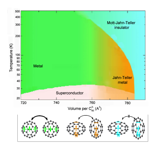
Figure 1: Experimental phase diagram of fcc-structured $\texttt{Rb}_{x}\texttt{Cs}_{3-x}\texttt{C}_{60}$, as a function of volume per $\texttt{C}_{60}$ experimentally obtained in zadik . Within the metallic (superconducting) regime, gradient shading from orange to green schematically illustrates crossover from the JTM to conventional metal. Lower panel: schematic depictions of the respective molecular electronic structure, intermolecular electron hopping, and JT molecular distortion for conventional metal, JT metal and MJT insulator in their interpretation.

The mechanism of superconductivity of the alkali-doped fullerides has not been fully understood. The positive correlation between $T_{c}$ and the lattice constant found in K- and Rb-doped fullerides has been understood in terms of the standard BCS theory: the density of states of conduction electrons is $\nu\propto 1/W$, and $T_{c}=1.14\langle\omega\rangle\exp(-1/\lambda\nu)$, thus the smaller $W$ the large $T_{c}$. Therefore superconductivity of $\texttt{A}_{3}\texttt{C}_{60}$ is often described with Eliashberg theory in terms of electron-phonon coupling and Tolmachev’s pseudopotential $\mu^{\ast}$ gun0 ; chen1 ; cap . In the same time there is another approach to describe phases of alkali-doped fulleride - the model of local pairing han1 ; han2 ; lam1 ; lam2 ; koga . The experimental basis for this hypothesis is the fact that the coherence length (size of a Cooper pair) in the superconducting alkali-doped fulleride is $\sim 2\ldots 3\texttt{nm}$, which is comparable with a size of a fullerene molecule $\texttt{C}_{60}$ $\sim 1\texttt{nm}$. Moreover, the Hubbard-like models predict that $\texttt{A}_{4}\texttt{C}_{60}$ is an anti-ferromagnetic insulator, while it is known experimentally that there are no moments in $\texttt{A}_{4}\texttt{C}_{60}$. The electrons in $\texttt{A}_{n}\texttt{C}_{60}$ relatively strong interact with Jahn-Teller intramolecular phonons with $H_{g}$ and $A_{g}$ symmetries. The interaction favors a low-spin state and might lead to a nonmagnetic insulator. At the same time there is, however, a Hund’s rule coupling, which favors a high-spin state. Thus competition between the Jahn-Teller coupling and the Hund’s rule coupling takes place. As a result each molecule $\texttt{C}_{60}^{3-}$ in $\texttt{Cs}_{3}\texttt{C}_{60}$ crystal (antiferromagnetic insulator) has spin $S=1/2$ instead $3/2$. Proceeding from these facts the local pairing model suggests that the electron-vibron interaction (interaction of electrons with $H_{g}$ and $A_{g}$ intramolecular Jahn-Teller oscillations) favors the formation of a local singlet: $\frac{1}{\sqrt{3}}\sum_{m}a_{im\uparrow}^{+}a_{im\downarrow}^{+}|0\rangle$, where the spin-up and spin-down electrons are situated on a site $i$ in the same quantum state $m$ (here $|0\rangle$ is the neutral $\texttt{C}_{60}$ molecule, the quantum number $m$ labels the three orthogonal states of $t_{1u}$ symmetry). The local singlet state competes with the normal state (high spin state) of two electrons $a_{im_{1}\uparrow}^{+}a_{im_{2}\uparrow}^{+}|0\rangle$ dictated by Hund’s rule. Using this assumption some important results have obtained. In a work suz the density of states in a band originated from $t_{1u}$ level has been calculated by applying the unrestricted Hartree-Fock approximation and the many body perturbation method. It has been found that $\texttt{A}_{2}\texttt{C}_{60}$ and $\texttt{A}_{4}\texttt{C}_{60}$ are nonmagnetic semiconductors and the band gaps in these materials are cooperatively formed by the electron-electron and electron-vibron interactions. On the other hand, it is difficult to predict within the model whether the following materials $\texttt{A}_{1}\texttt{C}_{60}$, $\texttt{A}_{3}\texttt{C}_{60}$ and $\texttt{A}_{5}\texttt{C}_{60}$ are metallic or not, it has been concluded at least that the materials are on the border of the metal-insulator transition. In the work gun1 it is conjectured that the Mott-Hubbard transition takes place for $U/W\sim\sqrt{N}$, where $N$ is an orbital degeneracy (for alkali-doped fullerides $N=3$) due to the matrix elements for the hoping of an electron or a hole from a site $i$ to a nearby site $j$ are enhanced as $\langle i|t_{ij}a^{+}_{im\sigma}a_{jm\sigma}|j\rangle=\sqrt{N}t$, thus the degeneracy increases $U_{c}$ (critical value of the on-site Coulomb repulsion such that if $U>U_{c}$ then a material is MI). In the same time in koch an analogous expression $\langle i|\widehat{H}|j\rangle=\sqrt{k}t$ has been obtained, but the factor $k$ depends on both the degeneracy and the filling $n$, so for $n=3$ the enhancement is $k=1.73$, for $n=2,4$ - $k=1.57$, for for $n=1,5$ - $k=1.21$. Thus the degeneracy contributes to the metallization of the systems. However, as pointed above, the conductivity depends on filling $n$ radically (for odd $n$ - metals, for even $n$ - insulators), therefore the competition between the Jahn-Teller effect and the Hund’s rule coupling must be accounted han1 .

In a work han2 it is shown that in $\texttt{A}_{3}\texttt{C}_{60}$ the local pairing is crucial in reducing the effects of the Coulomb repulsion. So, for the Jahn-Teller $H_{g}$ phonons the attractive interaction is overwhelmed by the Coulomb repulsion. Superconductivity remains, however, even for $U_{vib}\ll U$, and $T_{c}$ drops surprisingly slowly as $U$ is increased. The reason is as follows. For noninteracting electrons the hopping tends to distribute the electrons randomly over the molecular levels. This makes more difficult to add or remove an electron pair with the same quantum numbers $m$. However as $U$ is large $U>W$ the electron hopping is suppressed and the local pair formation becomes more important. Thus the Coulomb interaction actually helps the local pairing. This leads to new physics in the strongly correlated low-bandwidth solids, due to the interplay between the Coulomb and electron-vibron interactions. In a such system the Eliashberg theory breaks down because of the closeness to a metal-insulator transition. Because of the local pairing, the Coulomb interaction enters very differently for Jahn-Teller and non-Jahn-Teller models, and it cannot be easily described by a Coulomb pseudopotential $g-\mu^{\ast}$. Theoretical phase diagram for $\texttt{A}_{3}\texttt{C}_{60}$ systems has been obtained with the DMFT analysis in nom1 ; nom2 . There are three phase: the superconducting (SC) phase at low temperature, the normal phase at more high temperatures and the phase of paramagnetic MI at bigger volume per $\texttt{C}_{60}^{3-}$. In the same time the dome shape of the SC phase is absent in the theoretical diagram. In this model the s-wave superconductivity is characterized by a order parameter $\Delta=\sum_{m=1}^{3}\left\langle a_{im\downarrow}a_{im\uparrow}\right\rangle$, which describes intraorbital Cooper pairs for the $t_{1u}$ electrons, $m$ and $i$ are the orbital and site (=molecule) indices respectively (the site index in $\Delta$ has been omitted, because $\Delta$ does not depend on a site - the solution is homogenous in space). Superconducting mechanism is that in such a system we have $U^{\prime}>U$ ($U^{\prime}$ is interorbital repulsion and $U$ is intraorbital one) due to the el.-vib. interaction. Interesting observation is that the double occupancy $\left\langle n_{m\uparrow}n_{m\downarrow}\right\rangle$ on each molecule increases toward the Mott transition and it jumply increases in a point of transition from the metal phase to the MI phase. Conversely, the double occupancy $\left\langle n_{m\uparrow}n_{m^{\prime}\downarrow}\right\rangle$ and spin $S$ per molecule decrease toward the Mott transition and they jumply decrease (to $S=1/2$) in the point of transition from the metal phase to the insulator phase. In the same time the local pairs are not bipolarons because in metallic phase the polarons (polaron band) are absent up to the Mott transition and stable electron pairs are not observed above $T_{c}$.

The local pairing hypothesis is confirmed with quantum Monte Carlo simulations of low temperature properties of the two-band Hubbard model with degenerate orbitals koga . It have been clarified that the SC state can be realized in a repulsively interacting two-orbital system due to the competition between the intra- and interorbital Coulomb interactions: it must be $U<U^{\prime}$ for this. The s-wave SC state appears along the first-order phase boundary between the metallic and paired Mott states in the paramagnetic system. The exchange interaction $J$ destabilizes the SC state additionally. In hosh the phase portrait of $\texttt{A}_{3}\texttt{C}_{60}$ has been obtained using the DMFT in combination with the continuous-time quantum Monte Carlo method. In the theoretical diagram there are the dome shaped SC region and spontaneous orbital-selective Mott (SOSM) state, in which itinerant and localized electrons coexist and it is identified as JT metal by the authors. The SOSM state is stabilized near the Mott phase, while SC appears in the lower-$U$ region. The transition into the SOSM and AFM phases is of the first order. In the same time, as discussed above, the line of phase transition from JT metal to conventional metal is absent in the experimental phase diagram (the molecular distortions gradually increase as lattice expands), hence the JT metal is not a phase, unlike the MJT insulator which is separated from the metal state by a line of the first kind phase transition. In the theoretical phase diagram the characteristic vertical cutoff of the SC and metallic phases (at low temperature) by MJT insulator phase is absent or weakly expressed (a hysteresis behavior is observed near the Mott transition point), the SC phase extends far into the region of large $U/W$ where the SOSM phase occurs.

In the present work we are aimed to find conditions of formation of the local pairs on fullerene molecules, then, based on the local pairing hypothesis, considering the Coulomb correlations and the JT-distortion of the molecules, to propose a general approach to description of the properties of alkali-doped fullerides $\texttt{A}_{n}\texttt{C}_{60}$ ($\texttt{A}=\texttt{K},\texttt{Rb},\texttt{Cs}$, $n=1\ldots 5$), namely to demonstrate mechanism of superconductivity of $\texttt{A}_{3}\texttt{C}_{60}$, conductivity of $\texttt{A}_{n}\texttt{C}_{60}$ with $n=1,3,5$ and insulation of the materials with $n=2,4$ with the loss of antiferromagnetic properties, and to obtain analytically the phase diagram of $\texttt{A}_{3}\texttt{C}_{60}$ with fcc structure which should be close to the experimental phase diagram.

II Local pairing

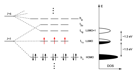
Figure 2: The molecular levels of $\texttt{C}_{60}$ close to the Fermi level. In a substance $\texttt{A}_{3}\texttt{C}_{60}$ the atoms of alkali metal $\texttt{A}=\texttt{K},\texttt{Rb},\texttt{Cs}$ give electrons to the LUMO of the fullerene molecule (red color). Right panel: corresponding band structure (density of state as a function of energy $E$ schematically).

Due to the quasispherical structure of the molecule $\texttt{C}_{60}$ the electron levels would be spherical harmonics with the angular momentum $l$, however the icosahedral symmetry generates the splits of the spherical states into icosahedral representation sav ; allon ; hadd . Fig.2 shows molecular levels close to the Fermi level. The LUMO is the 3-fold degenerate $t_{1u}$ orbital (i.e. it can hold up to six electrons). It is separated by about 1.5eV from the highest occupied molecular orbital (HOMO) and by about 1.2eV from the next unoccupied level (LUMO+1). The alkali-metal atoms give electrons to the empty $t_{1u}$ level so that the level becomes partly occupied. Hamiltonian of the system can be written in a form of three-orbital Hubbard Hamiltonian with the Hund coupling koga ; geor and the electron-vibron (Jahn-Teller phonons) interaction:

$$\widehat{H} = \sum_{ij}\sum_{m}\sum_{\sigma}\left(t_{ij}+(\varepsilon_{m}-\mu)\delta_{ij}\right)a^{+}_{im\sigma}a_{jm\sigma}+U\sum_{i}\sum_{m}\sum_{\sigma}n_{im\uparrow}n_{im\downarrow}$$ (1)

$$+ \left(U^{\prime}-J\right)\sum_{i}\sum_{m<m^{\prime}}\sum_{\sigma}n_{im\sigma}n_{im^{\prime}\sigma}+\left(U^{\prime}+J\right)\sum_{i}\sum_{m<m^{\prime}}\sum_{\sigma}n_{im\sigma}n_{im^{\prime}-\sigma}$$

$$+ V\sum_{\langle ij\rangle}\sum_{m,m^{\prime}}\sum_{\sigma\sigma^{\prime}}n_{im\sigma}n_{jm^{\prime}\sigma^{\prime}}+\widehat{H}_{el-vib}+\widehat{H}_{vib},$$

where $a^{+}_{im\sigma}(a_{im\sigma})$ is the electron creation (annihilation) operator in the orbital $m=1,2,3$ localized on the site $i$; $n_{im\sigma}=a^{+}_{im\sigma}a_{im\sigma}$ is the particle number operator; $\sigma(=\uparrow,\downarrow)$ is the spin index; $t_{ij}$ is the hopping integral between neighboring sites and the same orbitals (the bandwidth is $W=2z|t|$, where $z$ is the number of nearest neighbors), $t_{ii}=0$; $\varepsilon_{m}$ is the orbital energy; $\mu$ is the chemical potential, $\delta_{ij}=1$ if $i=j$, $\delta_{ij}=0$ if $i\neq j$; the energy $V$ is the Coulomb repulsion between neighboring sites ($i\neq j$):

$$V=\int d\textbf{r}d\textbf{r}^{\prime}|\phi_{m}^{i}(\textbf{r})|^{2}V_{c}^{ij}(\textbf{r},\textbf{r}^{\prime})|\phi_{m^{\prime}}^{j}(\textbf{r}^{\prime})|^{2},$$ (2)

where $V_{c}^{ij}(\textbf{r},\textbf{r}^{\prime})$ is a operator of cross-site Coulomb interaction; $U$ is the intra-orbital on-site Coulomb repulsion energy; $U^{\prime}$ is the inter-orbital on-site Coulomb repulsion energy; $J>0$ is the on-site exchange interaction energy:

$$U = \int d\textbf{r}d\textbf{r}^{\prime}|\phi_{m}(\textbf{r})|^{2}V_{c}(\textbf{r},\textbf{r}^{\prime})|\phi_{m}(\textbf{r}^{\prime})|^{2}$$ (3)

$$U^{\prime} = \int d\textbf{r}d\textbf{r}^{\prime}|\phi_{m}(\textbf{r})|^{2}V_{c}(\textbf{r},\textbf{r}^{\prime})|\phi_{m^{\prime}}(\textbf{r}^{\prime})|^{2}$$ (4)

$$J = \int d\textbf{r}d\textbf{r}^{\prime}\phi_{m}^{\ast}(\textbf{r})\phi_{m^{\prime}}^{\ast}(\textbf{r}^{\prime})V_{c}(\textbf{r},\textbf{r}^{\prime})\phi_{m}(\textbf{r}^{\prime})\phi_{m^{\prime}}(\textbf{r}),$$ (5)

where $V_{c}(\textbf{r},\textbf{r}^{\prime})$ is a operator of on-site Coulomb interaction. In a multi-orbital system the on-site Coulomb interaction is presented with two terms: density-density interaction energy $U$ ($U^{\prime}$ for different orbitals) and the energy of the double inter-orbital hoppings $\sum_{ll^{\prime}mm^{\prime}}\sum_{\sigma\sigma^{\prime}}J_{l^{\prime}m^{\prime}lm}a^{+}_{il^{\prime}\sigma}a^{+}_{im^{\prime}\sigma^{\prime}}a_{il\sigma}a_{im\sigma^{\prime}}$ (where $l^{\prime}\neq l,m^{\prime}\neq m$) feng . The hoppings’ energy cannot be reduced to the multiplication of operators of occupation numbers like the density-density energy $U^{\prime}\sum_{lm}\sum_{\sigma\sigma^{\prime}}n_{il\sigma}n_{im\sigma^{\prime}}$. However contribution of the exchange processes $Ja^{+}_{im\sigma}a^{+}_{il\sigma^{\prime}}a_{il\sigma}a_{im\sigma^{\prime}}$ can be reduced to the Hund coupling: variational calculations demonstrate that Coulomb energy of two electrons in a singlet state $|m_{1}\uparrow,m_{2}\downarrow\rangle$ is $U^{\prime}+J$ and in a triplet state $|m_{1}\uparrow,m_{2}\uparrow\rangle$ is $U^{\prime}-J$. For example, the first excited energy levels of a helium atom, which are parallel and antiparallel spin configurations, are separated from each other with energy gap $2J$. Physical reason of this level splitting is that antisymmetric in spatial variables wave function (parallel spins) of two electrons minimizes their Coulomb repulsion due to maximal separation of the electrons in space in comparison with state with the symmetric spatial part of wave function (antiparallel spins) where the electrons are closer to each other. This makes it possible to assume that the exchange processes give main contribution in the interaction energy, and contribution of other double inter-orbital hoppings can be neglected. Thus in this approximation we can write Coulomb interaction between electrons in a form of Hamiltonian (1) where the effective density-density interaction is present only. As a rule $U\gg J$, $U^{\prime}\simeq U-2J$ (the RPA interaction parameters for the family $\texttt{A}_{3}\texttt{C}_{60}$ taken from nom3 are $U\sim 0.82\texttt{eV},U^{\prime}\sim 0.76\texttt{eV},J\sim 31\texttt{meV}$). Then $U^{\prime}-J<U^{\prime}+J<U$ that means Hund’s rule: the electron configuration with minimal energy has maximal spin. Corresponding electron configurations for two electrons is shown in Fig.3.

In the $\texttt{C}_{60}^{n-}$ molecule the excess electrons are coupled strongly to two $A_{g}$ and eight $H_{g}$ intramolecular Jahn-Teller phonons (electron-vibron interaction). The operators of the el.-vib. interaction and the vibrons’ energy have forms accordingly han1 ; han2 ; suz ; gun ; tak :

$$\widehat{H}_{el-vib} = \lambda_{A_{g}}\sum_{i}\sum_{M=1}^{2}\sum_{m=1}^{3}\sum_{m^{\prime}=1}^{3}\sum_{\sigma}V^{(0)}_{mm^{\prime}}a^{+}_{im\sigma}a_{im^{\prime}\sigma}\left(b^{+}_{i0M}+b_{i0M}\right)$$ (6)

$$+ \lambda_{H_{g}}\sum_{i}\sum_{\nu=1}^{5}\sum_{M=1}^{8}\sum_{m=1}^{3}\sum_{m^{\prime}=1}^{3}\sum_{\sigma}V^{(\nu)}_{mm^{\prime}}a^{+}_{im\sigma}a_{im^{\prime}\sigma}\left(b^{+}_{i\nu M}+b_{i\nu M}\right),$$

$$\widehat{H}_{vib} = \sum_{i}\sum_{M=1}^{2}\omega_{M}b^{+}_{i0M}b_{i0M}+\sum_{i}\sum_{\nu=1}^{5}\sum_{M=1}^{8}\omega_{M}b^{+}_{i\nu M}b_{i\nu M},$$ (7)

where $\lambda_{A_{g}}$ and $\lambda_{H_{g}}$ are coupling constants to $A_{g}$ and $H_{g}$ intramolecular Jahn-Teller phonons respectively, the elements $V^{(\nu)}_{mm^{\prime}}$ of coupling matrices $\widehat{V}^{\nu}$ are determined by icosahedral symmetry. The matrix corresponding to $A_{g}$ phonons ($\nu=0$) is

$$V^{(0)}=\left(\begin{array}[]{ccc}1&0&0\\ 0&1&0\\ 0&0&1\\ \end{array}\right).$$ (8)

Coupling to $H_{g}$ phonons ($\nu=1\ldots 5$) is given by the matrixes

$$V^{(1)}=\frac{1}{2}\left(\begin{array}[]{ccc}-1&0&0\\ 0&-1&0\\ 0&0&2\\ \end{array}\right)\quad V^{(2)}=\frac{\sqrt{3}}{2}\left(\begin{array}[]{ccc}1&0&0\\ 0&-1&0\\ 0&0&0\\ \end{array}\right)\quad V^{(3)}=\frac{\sqrt{3}}{2}\left(\begin{array}[]{ccc}0&1&0\\ 1&0&0\\ 0&0&0\\ \end{array}\right)$$ (18)

$$V^{(4)}=\frac{\sqrt{3}}{2}\left(\begin{array}[]{ccc}0&0&1\\ 0&0&0\\ 1&0&0\\ \end{array}\right)\quad V^{(5)}=\frac{\sqrt{3}}{2}\left(\begin{array}[]{ccc}0&0&0\\ 0&0&1\\ 1&0&0\\ \end{array}\right).$$ (25)

Vibrational energies for the $A_{g}$ and $H_{g}$ modes are within the limits $\omega=200\ldots 1800\texttt{cm}^{-1}$ gun0 ; koch .

Figure 3: The configurations of two electrons on the 3-fold degenerate orbital. Ground state corresponds to configuration with parallel spins. The intraorbital configuration has the largest energy.

Figure 4: The configurations of three electrons on LUMO of a molecule $\texttt{C}_{60}$. Ground state corresponds to configuration with parallel spins. The configuration with a local pair (red color) has the largest energy.

According to the model of local pairing for superconductivity of $\texttt{A}_{3}\texttt{C}_{60}$ the interaction of electrons with $A_{g}$ and $H_{g}$ intramolecular oscillations favors the formation of a local singlet han1 ; han2 ; lam1 ; lam2 :

$$\frac{1}{\sqrt{3}}\sum_{m}a_{m\uparrow}^{+}a_{m\downarrow}^{+}|0\rangle,$$ (26)

where the spin-up and spin-down electrons have the same $m$ quantum number. Here $|0\rangle$ is the neutral $\texttt{C}_{60}$ molecule, the quantum number $m$ labels the three orthogonal states of $t_{1u}$ symmetry. In contrast, the normal state (high spin state) of two electrons is

$$\frac{1}{\sqrt{3}}\sum_{m_{1}<m_{2}}a_{m_{1}\uparrow}^{+}a_{m_{2}\uparrow}^{+}|0\rangle.$$ (27)

As noted in han2 , for noninteracting electrons the hopping tends to distribute the electrons randomly over the molecular levels. However if the on-site Coulomb repulsion $U$ is large so that $U>W$ the electron hopping is suppressed and the local pair formation becomes more important. Thus Coulomb interaction actually helps the local pairing and superconductivity is result of interplay between the el.-vib. interaction, the Coulomb blockade on a site and the hopping between neighboring sites. Superconductivity is expected to exist in this material right up to the Mott transition.

Based on the local pairing approach the Hamiltonian (1) can be simplified in the following manner. Fig.4 shows energies for different electron configurations of $\texttt{C}_{60}^{3-}$ molecule (that is for the molecule in $\texttt{A}_{3}\texttt{C}_{60}$ solid). We can see Hund’s rule: the electron configuration with maximal spin $S=3/2$ has minimal energy: $E_{3}-E_{1}=U-U^{\prime}+3J\simeq 5J>E_{2}-E_{1}=4J>0$. Thus the ground state of the system is a state $|m_{1}\sigma,m_{2}\sigma,m_{3}\sigma\rangle$, in order to form a local pair (26) the energy $E_{3}-E_{1}=U-U^{\prime}+3J$ must be expended. Therefore to study only the local pairing it is sufficient to measure the Coulomb energy of the local pairing configuration from the energy of the ground state (Hund’s rule configuration $|\uparrow\uparrow\uparrow\rangle$). Thus in this approach two electrons in the state $|m\uparrow m\downarrow\rangle$ on a fullerene molecule ”interact” with energy $U-U^{\prime}+3J$ which is the Hund coupling, but Coulomb correlation effects between electrons on neighboring molecules are neglected by the averaging. Then we can reduce the Hamiltonian (1) to a form:

$$\widehat{H}_{eff} = \frac{1}{2}\left(U^{\prime}-J\right)\sum_{i}\langle n_{i}\rangle\left(\langle n_{i}\rangle-1\right)+V\sum_{\langle ij\rangle}\langle n_{i}\rangle\langle n_{j}\rangle$$

$$+ \sum_{ij}\sum_{m}\sum_{\sigma}\left(t_{ij}+(\varepsilon_{m}-\mu)\delta_{ij}\right)a^{+}_{im\sigma}a_{jm\sigma}+\left(U-U^{\prime}+3J\right)\sum_{i}\sum_{m}n_{im\uparrow}n_{im\downarrow}+\widehat{H}_{el-vib}+\widehat{H}_{vib},$$

where $\langle n_{i}\rangle$ is an average occupation number of a site $i$. Thus the effective Coulomb repulsion $U-U^{\prime}+3J\sim 0.15\texttt{eV}$, which is much smaller than the on-site Coulomb repulsion $U\sim 0.8\texttt{eV}$, resists to the local pairing, unlike the usual Holstein-Hubbard model without degeneration.

We can eliminate the vibron variables using perturbation theory. Let the molecular vibrations occur with a certain frequency $\omega_{0}$. Since a vibron is localized on a molecule then el.-el interaction mediated by the exchange of a vibron has a form:

$$\widehat{H}_{el-el} = \sum_{i}\sum_{m,m^{\prime}}\sum_{\nu}\lambda^{2}_{\nu}V^{(\nu)}_{mm^{\prime}}V^{(\nu)}_{mm^{\prime}}a^{+}_{im\uparrow}a_{im^{\prime}\uparrow}a^{+}_{im\downarrow}a_{im^{\prime}\downarrow}$$ (29)

$$(-i)\int_{-\infty}^{+\infty}\left\langle 0\left|\widehat{T}\left\{\left(b_{\nu i}(t)+b_{\nu i}^{+}(t)\right)\left(b_{\nu i}+b_{\nu i}^{+}\right)\right\}\right|0\right\rangle dt,$$

where $\lambda_{0}=\lambda_{A_{g}}$, $\lambda_{\nu}=\lambda_{H_{g}}$ for $\nu=1\ldots 5$, $\widehat{T}$ is a Bose time-ordering operator, $b(t)=e^{i\omega_{0}b^{+}bt}be^{-i\omega_{0}b^{+}bt}$ is an annihilation (creation) phonon operator in Heisenberg representation, $|0\rangle$ is a zero-phonon state. Expression under integral is propagation of a vibron in a time $t$. The corresponding processes are shown in Fig.(5). Then

$$\widehat{H}_{el-el} = \sum_{i}\sum_{m,m^{\prime}}\sum_{\nu}\lambda^{2}_{\nu}V^{(\nu)}_{mm^{\prime}}V^{(\nu)}_{mm^{\prime}}a^{+}_{im\uparrow}a_{im^{\prime}\uparrow}a^{+}_{im\downarrow}a_{im^{\prime}\downarrow}$$ (30)

$$(-i)\int_{-\infty}^{+\infty}\left[\theta_{t}e^{-i\omega_{0}t}+\theta_{-t}e^{i\omega_{0}t}\right]dt=-\frac{2}{\omega_{0}}\sum_{i}\sum_{m,m^{\prime}}\sum_{\nu}\lambda^{2}_{\nu}V^{(\nu)}_{mm^{\prime}}V^{(\nu)}_{mm^{\prime}}a^{+}_{im\uparrow}a_{im^{\prime}\uparrow}a^{+}_{im\downarrow}a_{im^{\prime}\downarrow},$$

where $\theta_{t}=1$ if $t\geq 0$, $\theta_{t}=0$ if $t<0$. The same result we have in frequency representation of the vibron’s propagator:

$$\widehat{H}_{el-el} = \sum_{i}\sum_{m,m^{\prime}}\sum_{\nu}\lambda^{2}_{\nu}V^{(\nu)}_{mm^{\prime}}V^{(\nu)}_{mm^{\prime}}a^{+}_{im\uparrow}a_{im^{\prime}\uparrow}a^{+}_{im\downarrow}a_{im^{\prime}\downarrow}\frac{-i}{2\pi\omega_{0}}\int_{-\infty}^{+\infty}\frac{2\omega_{0}}{\omega^{2}-\omega^{2}_{0}+2i\delta\omega_{0}}d\omega$$ (31)

$$= -\frac{2}{\omega_{0}}\sum_{i}\sum_{m,m^{\prime}}\sum_{\nu}\lambda^{2}_{\nu}V^{(\nu)}_{mm^{\prime}}V^{(\nu)}_{mm^{\prime}}a^{+}_{im\uparrow}a_{im^{\prime}\uparrow}a^{+}_{im\downarrow}a_{im^{\prime}\downarrow}.$$

Figure 5: interaction between two electrons on a site $i$ mediated by the exchange of a vibron localized in this molecule: the case (a) corresponds to a direct process $\frac{2}{\omega_{0}}\sum_{\nu}\lambda^{2}_{\nu}V^{(\nu)}_{mm}V^{(\nu)}_{mm}a^{+}_{im\uparrow}a_{im\uparrow}a^{+}_{im\downarrow}a_{im\downarrow}$, the case (b) corresponds to an exchange process $\frac{2}{\omega_{0}}\sum_{\nu}\lambda^{2}_{\nu}V^{(\nu)}_{mm^{\prime}}V^{(\nu)}_{mm^{\prime}}a^{+}_{im\uparrow}a_{im^{\prime}\uparrow}a^{+}_{im\downarrow}a_{im^{\prime}\downarrow}$, where $m\neq m^{\prime}$. The picture (c) corresponds to the shift of electron’s energy due to the el.-vib. interaction on a site.

At nonzero temperature we should pass to complex time $it=\rightarrow\tau$, where $\tau=-1/T\ldots 1/T$. This is the same that to pass to complex frequency $\omega\rightarrow i\omega_{n}$, where $\omega_{n}=\pi nT$. Then Eq.(31) takes a form:

$$\widehat{H}_{el-el} = -\sum_{i}\sum_{m,m^{\prime}}\sum_{\nu}\lambda^{2}_{\nu}V^{(\nu)}_{mm^{\prime}}V^{(\nu)}_{mm^{\prime}}a^{+}_{im\uparrow}a_{im^{\prime}\uparrow}a^{+}_{im\downarrow}a_{im^{\prime}\downarrow}\frac{T}{\omega_{0}}\sum_{n=-\infty,n\neq 0}^{+\infty}\frac{2\omega_{0}}{(\pi nT)^{2}+\omega^{2}_{0}}$$ (32)

$$= -\frac{2}{\omega_{0}}\left[\coth\left(\frac{\omega_{0}}{T}\right)-\frac{T}{\omega_{0}}\right]\sum_{i}\sum_{m,m^{\prime}}\sum_{\nu}\lambda^{2}_{\nu}V^{(\nu)}_{mm^{\prime}}V^{(\nu)}_{mm^{\prime}}a^{+}_{im\uparrow}a_{im^{\prime}\uparrow}a^{+}_{im\downarrow}a_{im^{\prime}\downarrow}.$$

The addendum with $n=0$ is excluded from the sum, because it corresponds to scattering of electron on the thermal phonons, which do not influence on the pairing of electrons ginz . We can see that at $T\rightarrow 0$ Eq.(32) goes into Eq.(31) as $\frac{2\lambda^{2}}{\omega_{0}}\left(1-\frac{T}{\omega_{0}}\right)$, that is at increasing of temperature the effectiveness of el.-vib. interaction is decreasing. At $T\rightarrow\infty$ ($T\gg\omega_{0}$) the el.-el. coupling via vibrons is $\frac{2\lambda^{2}}{3T}\rightarrow 0$.

Thus we can see that the el.-el. interaction mediated by the exchange of vibrons can be reduced to BCS-like interaction (point, nonretarded) within single orbital $m$ that corresponds to diagonal elements of the matrixes $\widehat{V}^{(\nu)}$:

$$U_{vib}^{mmmm}=\frac{2}{\omega_{0}}\left[\coth\left(\frac{\omega_{0}}{T}\right)-\frac{T}{\omega_{0}}\right]\sum_{\nu}\lambda^{2}_{\nu}V^{(\nu)}_{mm}V^{(\nu)}_{mm}$$ (33)

and between different orbitals $m$ and $m^{\prime}$ that corresponds to the nondiagonal elements:

$$U_{vib}^{mm^{\prime}mm^{\prime}}=\frac{2}{\omega_{0}}\left[\coth\left(\frac{\omega_{0}}{T}\right)-\frac{T}{\omega_{0}}\right]\sum_{\nu}\lambda^{2}_{\nu}V^{(\nu)}_{mm^{\prime}}V^{(\nu)}_{mm^{\prime}}.$$ (34)

For simplicity we suppose that the interaction energies are the same for all orbitals $m$: $U_{vib}^{mmmm}=U_{vib}$ - direct (intraorbital) interaction, $U_{vib}^{mm^{\prime}mm^{\prime}}=J_{vib}$ - exchange (interorbital) interaction. It should be noticed that $J_{vib}>0$ as we can see using the matrixes (8,18). In addition we should consider the process $\sum_{\nu}\lambda^{2}_{\nu}V^{(\nu)}_{mm}V^{(\nu)}_{m^{\prime}m^{\prime}}a^{+}_{im\uparrow}a_{im\uparrow}a^{+}_{im^{\prime}\downarrow}a_{im^{\prime}\downarrow}$ which corresponds to the direct interorbital interaction $U_{vib}^{\prime}\propto\sum_{\nu}\lambda^{2}_{\nu}V^{(\nu)}_{mm}V^{(\nu)}_{m^{\prime}m^{\prime}}$. However, using the matrixes (8,18) we can see that $A_{g}$ and $H_{g}$ phonons give contribution to the interaction $U_{vib}^{mmm^{\prime}m^{\prime}}$ with different signs: $V^{0}_{mm}V^{0}_{m^{\prime}m^{\prime}}=1$, $\sum_{\nu=1}^{5}V^{(\nu)}_{mm}V^{(\nu)}_{m^{\prime}m^{\prime}}=-1/2$, unlike the intraorbital and the exchange interorbital interactions. Hence it is possible to choose such values of the coupling constants $\lambda_{A_{g}}$ and $\lambda_{H_{g}}$ so that $U_{vib}^{\prime}=0$ (for example, $\lambda_{H_{g}}=2\lambda_{A_{g}}$ for the model with the same frequency $\omega_{0}$). Thus this interaction can be much weaker than $U_{vib}$ and $J_{vib}$, that is confirmed by numerical calculation for vibron-mediated interactions in $\texttt{Cs}_{3}\texttt{C}_{60}$ nom4 . Then the Hamiltonian (II) takes a form:

$$\widehat{H}_{eff} = \sum_{ij}\sum_{m}\sum_{\sigma}\left(t_{ijmm}+(\varepsilon_{m}-\mu)\delta_{ij}\right)a^{+}_{im\sigma}a_{jm\sigma}$$ (35)

$$+ \left(U-U^{\prime}+3J-U_{vib}\right)\sum_{i}\sum_{m}n_{im\uparrow}n_{im\downarrow}-J_{vib}\sum_{i}\sum_{m^{\prime}\neq m}a_{im\uparrow}^{+}a_{im^{\prime}\uparrow}a_{im\downarrow}^{+}a_{im^{\prime}\downarrow},$$

where we have omitted the constant contribution in energy (the first and the second terms in Eq.(II)) and the vibrons’ energy $\widehat{H}_{vib}$. If each molecule is isolated, that is $t_{ij}=0$, and the el.-vib. interaction is stronger than the Hund coupling, that is $U-U^{\prime}+3J-U_{vib}-2J_{vib}<0$, then the anti-Hund distribution of electrons over orbitals occurs (the low-spin state (26)). Turning on the hopping $t_{ij}\neq 0$ between molecules the electrons are collectivized and they aspire to distribute randomly over the molecular levels. Then the local pairing (26) is determined by presence of the anomalous averages $\langle a_{im\downarrow}a_{im\uparrow}\rangle$ and $\langle a_{im\uparrow}^{+}a_{im\downarrow}^{+}\rangle$, which are determined self-consistently over the entire system. To find the anomalous averages we should distinguish them in Eq.(35), then the Hamiltonian takes a following form:

$$\widehat{H}_{eff} = \sum_{ij}\sum_{mm^{\prime}}\sum_{\sigma}\left(t_{ij}^{mm}+(\varepsilon_{m}-\mu)\delta_{ij}\right)a^{+}_{im\sigma}a_{jm\sigma}$$ (36)

$$+ \sum_{i}\sum_{m}\left[\Delta_{m}^{+}a_{im\uparrow}a_{im\downarrow}+\Delta_{m}a_{im\downarrow}^{+}a_{im\uparrow}^{+}\right]$$

$$+ (U_{vib}-U+U^{\prime}-3J)\sum_{i}\sum_{m}\langle a_{im\uparrow}^{+}a_{im\downarrow}^{+}\rangle\langle a_{im\downarrow}a_{im\uparrow}\rangle+J_{vib}\sum_{i}\sum_{m^{\prime}\neq m}\langle a_{im^{\prime}\uparrow}^{+}a_{im^{\prime}\downarrow}^{+}\rangle\langle a_{im^{\prime}\downarrow}a_{im^{\prime}\uparrow}\rangle$$

where

$$\Delta_{m} = \frac{U_{vib}-U+U^{\prime}-3J}{N}\sum_{i}\langle a_{im\downarrow}a_{im\uparrow}\rangle+\frac{J_{vib}}{N}\sum_{i}\sum_{m^{\prime}\neq m}\langle a_{im^{\prime}\downarrow}a_{im^{\prime}\uparrow}\rangle$$

$$\Delta_{m}^{+} = \frac{U_{vib}-U+U^{\prime}-3J}{N}\sum_{i}\langle a_{im\uparrow}^{+}a_{im\downarrow}^{+}\rangle+\frac{J_{vib}}{N}\sum_{i}\sum_{m^{\prime}\neq m}\langle a_{im^{\prime}\uparrow}^{+}a_{im^{\prime}\downarrow}^{+}\rangle$$ (37)

is the order parameter. $N$ is the number of lattice sites (number of the molecules). Eq.(II) means that the order parameter in such system is determined by the local pairing. It should be noticed that the condensates $\langle a_{im\downarrow}a_{im\uparrow}\rangle$ for different orbitals $m$ have the same phase because $J_{vib}>0$. In this model the exchange energy $3J$ and the difference $U-U^{\prime}\sim 2J$ resists the attraction energies $U_{vib},J_{vib}$. As indicated above the exchange energy $J$ is much less than Coulomb repulsion $U,U^{\prime}$. Thus for the local pairing a weaker condition $U_{vib}\gtrsim 5J$ than $U_{vib}\gtrsim U$ must be satisfied. The average number of electrons per site

$$\sum_{m}\langle n_{m}\rangle=\frac{1}{N}\sum_{i}\sum_{m}\sum_{\sigma}\langle a_{im\sigma}^{+}a_{im\sigma}\rangle$$ (38)

is determined by the position of the chemical potential $\mu$, and $\langle\ldots\rangle=\Xi^{-1}Tr\ldots\exp(-\widehat{H}/T)$ denotes averaging procedure where $\Xi$ is a partition function.

The effective Hamiltonian (II) does not account Coulomb correlations between electrons on neighboring sites, therefore to study conduction or insulation of the material we should proceed from the full Hamiltonian (1). The on-site Coulomb repulsions $U,U^{\prime}$, the on-site exchange interaction energy $J$ and the Coulomb repulsion between neighboring sites $V$ determine the change of energy at transfer of an electron from a site to a nearby site. This process is shown in Fig.6a. We can see that the energy change in this process is

$$\Delta E_{\texttt{Hund}}=E_{2}-E_{1}=U+4J-V,$$ (39)

where $E_{1}$ is energy of an initial electron configuration (the Hund’s rule) of neighboring sites, $E_{2}$ is energy of the configuration if to transfer an electron from the site to another. A band conductor becomes insulator if an electron does not have enough reserve of kinetic energy (which is a bandwidth $W$) to overcome the Coulomb blockade on a site: $\Delta E>W$. In the absence of long-range order all numerical and analytical calculations indicate that the Mott-Hubbard transition should occur in the region $0.5W<U_{c}<1.7W$ gebh , so in Hubbard-III-like analytical calculation of the superconducting critical temperature in the presence of local Coulomb interactions a critical value $U_{c}=W$ can be used rod . Thus we can assume that a band conductor becomes the Mott insulator if

$$\frac{\Delta E}{W}\geqslant 1.$$ (40)

For example, let us consider $\texttt{Rb}_{3}\texttt{C}_{60}$. According to nom3 $W=0.454\texttt{eV},U=0.92\texttt{eV},J=34\texttt{meV},V=0.27\texttt{eV}$, then $\Delta E/W=1.73$. This means that $\texttt{Rb}_{3}\texttt{C}_{60}$ would have to be the Mott insulator. However $\texttt{Rb}_{3}\texttt{C}_{60}$ is a conductor and, at low temperatures, is a superconductor even. As discussed above, the results of gun1 ; koch state that the degeneracy and the filling contribute to the metallization of the systems due to the matrix elements for the hopping of an electron or a hole from a site $i$ to a nearby site $j$ are enhanced as $\langle i|t_{ij}a^{+}_{im\sigma}a_{jm\sigma}|j\rangle=\sqrt{k}t$ where $k>1$. However, it should be noted, that in a single-orbital system the bandwidth $W$ is determined by the hopping as $W=2z|t|$, where $z$ is number of the nearest neighbors. As stated above in multi-orbital system the hopping is renormalized as $t\rightarrow\sqrt{k}t$, hence the observed bandwidth $W$ has to be determined with the renormalized hopping. Therefore the degeneracy cannot change the criterium (40) which is determined with the energetic balance. The degeneracy and the filling essentially influence on the metal-insulator transition in a multi-orbital system but due to configuration energy in $\Delta E$ as will be demonstrated below.

Accounting of the el.-vib. interaction can change the situation. As we can see from Eq.(35) for 3-fold degenerate level $t_{1u}$ each pair obtains energy $-U_{vib}-2J_{vib}$ due to interaction within own orbital (for example $m=1$) $1\leftrightarrow 1$ with energy $-U_{vib}$ and due to interorbital coupling with other two orbitals $1\leftrightarrow 2,1\leftrightarrow 3$ with energy $-J_{vib}$ for each. Formation of the local pair is possible if electron configuration with the pair has energy which is less than energy of electron configuration according to the Hund’s rule (see Fig.4): $U-U^{\prime}+3J-U_{vib}-2J_{vib}<0$. Then the change of energy at transfer of an electron from a site to the nearby site is

$$\Delta E_{\texttt{anti-Hund}}=E_{2}-E_{1}=U-V-U_{vib}-2J_{vib},$$ (41)

as shown in Fig.6b. Here we can see more favorable situation for conductivity because $\Delta E$ in this case is less than in a case of the Hund’s rule configuration (39) due to configuration (exchange) energy $4J$ and the el.-vib. interaction. However in the normal state (metallic) the anomalous averages are absent: $\langle a_{im\downarrow}a_{im\uparrow}\rangle=0$ and $\langle a_{im\uparrow}^{+}a_{im\downarrow}^{+}\rangle=0$. This means the local pair configuration is absent at the initial stage and we have the transfer of an electron according to Hund’s rule but with el.-vib. interaction

$$\Delta E_{\texttt{Hund}}=U+4J-V-U_{vib}-2J_{vib},$$ (42)

where the local pair is formed on the second site - Fig.6a. But $\Delta E_{\texttt{Hund}}>\Delta E_{\texttt{anti-Hund}}$ due to configuration (exchange) energy $4J$. Then it can be that $\Delta E_{\texttt{Hund}}/W>1$ and $\Delta E_{\texttt{anti-Hund}}/W<1$. Hence transition from SC state to the normal state would be transition to MI. However the normal state is conducting due to following mechanism. Let $\Delta E_{\texttt{Hund}}/W>1$ hence the hopping between molecules is blocked and electrons are locked on a molecule. In the same time $U-U^{\prime}+3J-U_{vib}-2J_{vib}<0$, hence on the isolated molecule the local pairing configuration is set. Then we obtain situation as in Fig.6b where $\Delta E_{\texttt{anti-Hund}}/W<1$, that allows an electron is transferred on the nearby molecule. This makes the normal state to be conducting. Thus if the energy is such that $\Delta E_{\texttt{anti-Hund}}/W<1$, then the material becomes conductor and superconductor at low temperatures. In Fig.6b we can see formation of configurations $\texttt{C}_{60}^{2-}$ and $\texttt{C}_{60}^{4-}$ with zero spins in the process of charge transferring. These configurations give a gain in JT energy (all electrons are in the pairs with energy $-U_{vib}-2J_{vib}$ each) but increase the Coulomb energy of a crystal. Therefore these configurations would be formed within the metal on very short time scales that do not imply static charge segregation, that corresponds to the results of spin-lattice relaxation measurements alloul1 ; alloul2 . As it will be demonstrated in Section IV for the even systems, i.e. $\texttt{A}_{n}\texttt{C}_{60}$ with $n=2,4$, the configurations $\texttt{C}_{60}^{2-}$ and $\texttt{C}_{60}^{4-}$ are stabilized that leads to insulation of these materials.

It should be noted that the local pair is not a local boson. Following dzum1 if the size of a local pair $a_{p}$ is much larger than the mean distance $R_{p}$ between the pairs then the bosonization of such local pairs cannot be realized due to their strong overlapping. Thus for fermionic nature of the pair it should be $a_{p}/R_{p}>1$. Using the uncertainty principle, the size of the local pair is defined as $a_{p}(T)=\left(\frac{\hbar}{2|\Delta|}\right)\sqrt{\varepsilon_{F}/2m}$, where the energy gap $|\Delta|$ plays role the binding energy in a pair. The size is compared with $R_{p}=(3/4\pi n_{p})^{1/3}$, where $n_{p}$ is the density of the pairs (half density of particles which is determined by Fermi energy $\varepsilon_{F}=\frac{\hbar^{2}}{2m}\left(\frac{3\pi^{2}N}{V}\right)^{2/3}\Rightarrow R_{p}\sim\sqrt[3]{V/N}\sim\hbar/\sqrt{\varepsilon_{F}m}$). Then we have

$$\frac{a_{p}}{R_{p}}\sim\frac{\varepsilon_{F}}{|\Delta|}\sim\frac{W}{|\Delta|}\quad\begin{array}[]{cc}\gg 1&\texttt{Cooper pairs}\\ \sim 1&\texttt{crossover from BCS to BEC}\\ \ll 1&\texttt{compact bosons}\\ \end{array}$$ (43)

Maximal $T_{c}$ of alkali-doped fullerides is $35\texttt{K}$, then $|\Delta|\approx 1.76T_{c}=62\texttt{K}\ll W\approx 0.5\texttt{eV}$. Thus the size of a pair is larger than average distance electrons and the pair is smeared over the crystal. That is in the metallic phase the local pairs have fermionic nature. At the border of transition to the MJT insulator the bosonization of local pairs occurs due to Coulomb blockage of hopping of electron between neighboring molecules. Thus electron configuration with the local pairs is a dynamical configuration of all molecules unlike the statical one with a compact local pair on each molecule for the MJT insulator state.

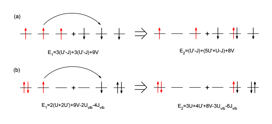
Figure 6: The transfer of a charge from a site to a nearby site. $E_{1}$ and $E_{2}$ are the energies of the electron configurations before and after the transfer. (a) - the transfer of an electron between sites with Hund’s electron configuration without el.-vib. interaction, (b) - the transfer of an electron between sites with the local pairs configuration.

Since the local pairs smeared over the crystal the anomalous averages $\langle a_{i\uparrow}a_{i\downarrow}\rangle$ exist in momentum space too: $\langle a_{-\textbf{k}\downarrow}a_{\textbf{k}\uparrow}\rangle$, and the BCS-like theory can be applied for description of the superconducting state of alkali-doped fullerides. Following a work litak , we can make transition from the site representation (36) into the reciprocal (momentum) space using relations:

$$a_{\textbf{k}m\sigma}=\frac{1}{\sqrt{N}}\sum_{j}e^{i\textbf{kr}_{j}}a_{jm\sigma},\quad a_{jm\sigma}=\frac{1}{\sqrt{N}}\sum_{j}e^{-i\textbf{kr}_{j}}a_{\textbf{k}m\sigma},$$ (44)

then we obtain the effective Hamiltonian like Hamiltonian of a multi-band superconductor:

$$\widehat{H}_{eff} = \sum_{m}\sum_{\textbf{k}}\sum_{\sigma}\xi_{m}(k)a^{+}_{\textbf{k}m\sigma}a_{\textbf{k}m\sigma}$$ (45)

$$+ \sum_{\textbf{k}}\sum_{m}\left[\Delta_{m}^{+}a_{\textbf{k}m\uparrow}a_{-\textbf{k}m\downarrow}+\Delta_{m}a_{-\textbf{k}m\downarrow}^{+}a_{\textbf{k}m\uparrow}^{+}\right],$$

with $\xi_{m}(k)=\varepsilon_{m}(k)-\mu$, and two last terms in Eq.(36) have been omitted as a constant. The homogeneous equilibrium gaps are defined as

$$\Delta_{m} = \frac{U_{vib}-U+U^{\prime}-3J}{N}\sum_{\textbf{k}}\langle a_{-\textbf{k}m\downarrow}a_{\textbf{k}m\uparrow}\rangle+\frac{J_{vib}}{N}\sum_{\textbf{k}}\sum_{m^{\prime}\neq m}\langle a_{-\textbf{k}m^{\prime}\downarrow}a_{\textbf{k}m^{\prime}\uparrow}\rangle$$

$$\Delta_{m}^{+} = \frac{U_{vib}-U+U^{\prime}-3J}{N}\sum_{\textbf{k}}\langle a_{\textbf{k}m\uparrow}^{+}a_{-\textbf{k}m\downarrow}^{+}\rangle+\frac{J_{vib}}{N}\sum_{\textbf{k}}\sum_{m^{\prime}\neq m}\langle a_{\textbf{k}m^{\prime}\uparrow}^{+}a_{-\textbf{k}m^{\prime}\downarrow}^{+}\rangle,$$ (46)

and the average number of electrons per site is

$$\sum_{m}\langle n_{m}\rangle=\frac{1}{N}\sum_{\textbf{k}}\sum_{m}\sum_{\sigma}\langle a_{\textbf{k}m\sigma}^{+}a_{\textbf{k}m\sigma}\rangle$$ (47)

Equations (II) and (47) should be solved self-consistently. It is easy to find that

$$\langle a_{-\textbf{k}m\downarrow}a_{\textbf{k}m\uparrow}\rangle=\frac{\Delta_{m}}{2E_{m}}\tanh\frac{E_{m}}{2T}$$ (48)

and

$$\langle a_{\textbf{k}m\sigma}^{+}a_{\textbf{k}m\sigma}\rangle=\frac{1}{2}\left(1-\frac{\xi_{m}(k)}{E_{m}}\tanh\frac{E_{m}}{2T}\right),$$ (49)

where $E_{m}=\sqrt{\xi_{m}(k)+\Delta_{m}^{2}}$. Thus a system with the local pairing $\langle a_{im\downarrow}a_{im\uparrow}\rangle$ is equivalent to a multi-band superconductor with a continual pairing $\langle a_{-\textbf{k}m\downarrow}a_{\textbf{k}m\uparrow}\rangle$ in each band. The multi-band theory asker1 ; asker2 ; asker3 can be mapped onto an effective single-band problem grig2 . Thus the three-orbitals $t_{1u}$ system can be reduced to an effective single-band superconductor, the more so that the condensates $\langle a_{-\textbf{k}m\downarrow}a_{\textbf{k}m\uparrow}\rangle$ for different orbitals $m$ have the same phase because $J_{vib}>0$. If to suppose the dispersion law of electrons in $t_{1u}$ conduction band $\xi_{m}(k)$ is the same for all orbitals $m$: $\xi_{1}=\xi_{2}=\xi_{3}=\xi$, then from Eq.(II) we obtain a simple equation for critical temperature:

$$\left|\begin{array}[]{ccc}\left(U_{vib}-U+U^{\prime}-3J\right)\zeta-1&J_{vib}\zeta&J_{vib}\zeta\\ J_{vib}\zeta&\left(U_{vib}-U+U^{\prime}-3J\right)\zeta-1&J_{vib}\zeta\\ J_{vib}\zeta&J_{vib}\zeta&\left(U_{vib}-U+U^{\prime}-3J\right)\zeta-1\\ \end{array}\right|=0$$ (53)

$$\Longrightarrow\left(U_{vib}+2J_{vib}-U+U^{\prime}-3J\right)\zeta=1,$$ (54)

where

$$\zeta=\frac{1}{N}\sum_{\textbf{k}}\frac{1}{2\xi(k)}\tanh\frac{\xi(k)}{2T_{c}}$$ (55)

In the alkali doped fulerides the conduction band is narrow $W=0.3\ldots 0.5\texttt{eV}$ and energies of vibrons are large $\omega\sim 0.2eV$, thus almost all electrons take part in el.-vib. interaction ($2\omega\sim W$), unlike electrons in conventional metals where only electrons near Fermi surface interact via phonons because $\omega\ll W$ there. Hence the final results are weakly sensitive to distribution of the density of states in conduction band, that is some averaged density can be used in this case, unlike conventional conductors where the results strongly depend on the density on Fermi level. Thus we can suppose the density of states in the conduction band is a constant $\nu=\nu_{0}$ if $-W/2<\xi<W/2$, otherwise $\nu=0$. Since $\sum_{\textbf{k}}\langle n(\textbf{k})\rangle=V\int\nu(\xi)d\xi$ it can be seen from Eq.(47) that

$$3=\sum_{m}\langle n_{m}\rangle=2\frac{V}{N}\sum_{m}\int_{-W/2}^{0}\nu_{0}d\xi\Longrightarrow\nu_{0}=\frac{N}{V}\frac{1}{W}.$$ (56)

Then Eq.(53) is reduced to a form

$$1=(g-\mu_{c})\int_{-\Omega}^{\Omega}\frac{1}{2\xi}\tanh\frac{\xi}{2T_{c}}d\xi,$$ (57)

where the integration is restricted by energy $\Omega=\min(\omega_{0},W/2)$ proceeding from the rectangular approximation for the density of states in conduction band, narrowness of conduction band and large vibron’s energy, for example for $\texttt{Cs}_{3}\texttt{C}_{60}$ at normal pressure the bandwidth is $W=0.341\texttt{eV}<2\omega_{0}\approx 0.4\texttt{eV}$. The coupling constant $g$ is determined with el.-vib. interaction $U_{vib}+2J_{vib}$, and the Coulomb pseudopotential $\mu_{c}$ is determined with the Hund coupling $U-U^{\prime}+3J$:

$$g=\frac{U_{vib}+2J_{vib}}{W}=\frac{\widetilde{U}_{vib}}{W},\quad\mu_{c}=\frac{U-U^{\prime}+3J}{W}.$$ (58)

The therm $\widetilde{U}_{vib}\equiv U_{vib}+2J_{vib}$ corresponds to the energy of attraction in a pair as discussed above. The bandwidth of alkali-doped fullerides is $W\sim 0.5\texttt{eV}$, the energy gap is $\Delta\approx 2T_{c}\sim 30\ldots 60\texttt{K}\ll\varepsilon_{F}=W/2$ that is a change of the chemical potential at transition to SC state can be neglected unlike the systems with the strong attraction and low particle density, where it can be $\Delta>\varepsilon_{F}$ and the change of the chemical potential plays important role in formation of SC state lok . On the other hand the vibrational energies for the $A_{g}$ and $H_{g}$ modes are $\omega_{0}\sim 0.2\texttt{eV}\sim\varepsilon_{F}$ that means Tolmachev’s weakening of the Coulomb pseudopotential by a factor $\ln\frac{\varepsilon_{F}}{\omega}$ does not take place.

It should be noticed that the effect of weak renormalization of electron’s mass due to el.-vib. interaction, which is similar to the effect in ordinary metals due to el.-phon. interaction, should be absent in alkali-doped fullerides. As shown in jones the renormalization is consequence of el.-phon. interaction and of the fact that the total momentum of the system

$$\textbf{P}^{\texttt{tot}}=\textbf{p}+\sum_{\textbf{q}}b_{\textbf{q}}^{+}b_{\textbf{q}}\hbar\textbf{q}$$ (59)

is a constant of the motion. Here p is the momentum of an electron, q is the wave vector of a phonon. The electron energy is renormalized as

$$E=E_{0}-\alpha\omega_{0}+\frac{p^{2}}{2m}\frac{1}{1+\alpha/6},$$ (60)

where $\alpha\sim\frac{\lambda^{2}}{\omega_{0}^{2}}$. However in alkali-doped fullerides electrons interact with internal oscillations (vibrons) of the fullerene molecules. Each vibron is localized on own molecule and cannot propagate to nearby molecules, unlike phonons in metals which propagate throw the system as waves. This means that the wave vector q is not quantum number for vibrons and Eq.(59) does not have physical sense. Then the electron’s momentum p should conserves separately. Moreover unlike conventional metals, where $U/W\ll 1$, the alkali-doped fullerides are strongly correlated systems, where $U/W\sim 1$, therefore the renormalization of the density of state is caused by the Coulomb correlations at presence of the el.-vib. interaction, that will be discussed in the next section.

In the same time in our case the shift of the electron’s energy $-\alpha\omega_{0}$ is a consequence of a process of el.-vib. interaction on a cite like the el.-el. interaction via vibrons considered above. This process is shown in Fig.(5c). Since a vibron is localized on a molecule we can write the energy shift using Eq.(6) and the averaging analogously to Eqs.(29,31):

$$\widehat{H}_{el.-vib.} = \sum_{i}\sum_{m,m^{\prime}}\sum_{\nu}\lambda^{2}_{\nu}V^{(\nu)}_{mm^{\prime}}V^{(\nu)}_{mm^{\prime}}a^{+}_{im\uparrow}a_{im\uparrow}\frac{i}{2\pi}\int_{-\infty}^{+\infty}\frac{2\omega_{0}}{\omega^{2}-\omega^{2}_{0}+2i\delta\omega_{0}}\frac{1}{\varepsilon-\omega-\varepsilon_{m^{\prime}}+i\delta}d\omega$$ (61)

$$=_{\varepsilon=\varepsilon_{m^{\prime}}} -\sum_{i}\sum_{m,m^{\prime}}\sum_{\nu}\frac{\lambda^{2}_{\nu}}{\omega_{0}}V^{(\nu)}_{mm^{\prime}}V^{(\nu)}_{mm^{\prime}}a^{+}_{im\uparrow}a_{im\uparrow}.$$

Expressions under the integral are propagator of a vibron and propagator of an electron located on a molecular level $\varepsilon_{m}$ (if we suppose $\varepsilon_{m}>0$ then $\delta\rightarrow+0$, if $\varepsilon_{m}<0$ then $\delta\rightarrow-0$). After calculation of the integral we have switched to the mass surface $\varepsilon=\varepsilon_{m}$. Thus interaction of an electron with the vibron field on a molecule shifts the electron’s energy as

$$-\sum_{m^{\prime}}\sum_{\nu}\frac{\lambda^{2}_{\nu}}{\omega_{0}}V^{(\nu)}_{mm^{\prime}}V^{(\nu)}_{mm^{\prime}},$$ (62)

whose modulus is the binding energy of an electron with deformation of a molecule if the electron is localized on it.

III Phase diagram

III.1 Influence of Coulomb correlations

The BCS formula (57) do not account Coulomb correlations between electrons on neighboring sites because it has been obtained using the effective Hamiltonian (35). For studying of these phenomena we should proceed from the full Hamiltonian (1). The correlations are determined by the fact that in order to transfer an electron from a site to a nearby site we have to change the energy of the configuration as in Fig.6b. On the other hand the possibility of this transferring determines metallic properties of the material - Eqs.(39,40,41). The Coulomb correlations can be accounted with Gutzwiller-Brinkman-Rice approach brink by the following manner. Quasiparticle states are determined with the pole expression of an electron propagator:

$$G(\textbf{k},\varepsilon)=\frac{Z}{\varepsilon-\xi(k)+i\gamma_{k}},$$ (63)

where $0<Z\leq 1$ is the discontinuity in the single-particle occupation number $n_{\textbf{k}}$ at the Fermi surface, in other hand the function $Z$ determines intensity of the quasiparticle peak at $\omega=0$ of a spectral function $A(\omega)=\sum_{\textbf{k}}A(\textbf{k},\omega)$, where $A(\textbf{k},\omega)=-\frac{1}{\pi}\texttt{Im}G(\textbf{k},\omega)\approx\frac{Z}{\pi}\frac{\gamma_{k}}{(\omega-\xi(k))^{2}+\gamma_{k}^{2}}$. For noninteracting electrons $Z=1$. At transition from metal state to MI state the peak disappears and in its place an energetic gap appears separating two Hubbard subbands. The vanishing of $Z$ therefore marks the metal-insulator transition bulla . Such Coulomb correlations redistribute the density of state in a conduction band. However in alkali-doped fullerides the el.-vib. interaction takes the whole bandwidth $2\omega_{0}\sim W$ hence the effective density of state is determined by the bandwidth $\nu_{F}\sim 1/W$ up to the appearance of the Hubbard subbands. In the Brinkman-Rice approach the renormalization parameter $Z$ is obtained as

$$Z=1-\left(\frac{\Delta E}{\Delta E_{c}}\right)^{2}=1-\left(\frac{U-V-\widetilde{U}_{vib}}{W}\right)^{2},$$ (64)

where $\Delta E_{c}$ is a critical energy change at transfer of an electron from a site to a nearby site. The last part of this formula is written for our model - Eqs.(39,40,41). Then the condition (40) is $Z\leq 0$. Using the propagator (63) we can obtain normal and anomalous Green functions from Gorkov’s equation:

$$G(\varepsilon_{n},\xi)=i\frac{Z\cdot\left(i\varepsilon_{n}+\xi\right)}{(i\varepsilon_{n})^{2}-\xi^{2}-Z^{2}|\Delta|^{2}}$$ (65)

$$F(\varepsilon_{n},\xi)=i\frac{Z^{2}\Delta}{(i\varepsilon_{n})^{2}-\xi^{2}-Z^{2}|\Delta|^{2}},$$ (66)

where $\varepsilon_{n}=\pi T(2n+1)$. Then the self-consistency condition for the order parameter is

$$\Delta=(g-\mu)T\sum_{n=-\infty}^{\infty}\int_{-\Omega}^{\Omega}d\xi iF(\varepsilon_{n},\xi)\Longrightarrow 1=(g-\mu)Z^{2}\int_{-\Omega}^{\Omega}\frac{1}{2\xi}\tanh\frac{\xi}{2T_{c}}d\xi,$$ (67)

where $\Omega=\min(\omega_{0},W/2)$ as discussed above. This formula for the critical temperature $T_{c}$, unlike the formula (57), accounts the Coulomb correlations through the renormalization parameter $Z$. For uncorrelated metal $Z=1$, at the transition to MI $Z=0$. Thus Coulomb correlations suppress the critical temperature.

Table 1: Calculated in nom3 bandwidth $W$, cRPA screened Coulomb parameters $U$, $U^{\prime}$, $J$, $V$ and dielectric constant $\varepsilon$ for the compounds with fcc-lattice: K, Rb and Cs in superconducting phases with maximum $T_{c}$ (at pressure $7\texttt{kbar}$), in the vicinity of the metal-insulator transition ($2\texttt{kbar}$) and in the antiferromagnetic insulating phase (normal pressure), respectively. At the bottom of the table the Coulomb barrier $U-U^{\prime}+3J$ for the local pairing is calculated.

	$K_{3}\texttt{C}_{60}$	$\texttt{Rb}_{3}\texttt{C}_{60}$	$\texttt{Cs}_{3}\texttt{C}_{60}$ (7kbar)	$\texttt{Cs}_{3}\texttt{C}_{60}$ (2kbar)	$\texttt{Cs}_{3}\texttt{C}_{60}$
volume per $\texttt{C}_{60}$ $(\texttt{A}^{3})$	722	750	762	784	804
$W(\texttt{eV})$	0.502	0.454	0.427	0.379	0.341
$U(\texttt{eV})$	0.82	0.92	0.94	1.02	1.08
$U^{\prime}(\texttt{eV})$	0.76	0.85	0.87	0.94	1.00
$J(\texttt{meV})$	31	34	35	35	36
$V(\texttt{eV})$	0.24 $-$ 0.25	0.26 $-$ 0.27	0.27 $-$ 0.28	0.28 $-$ 0.29	0.30
$\varepsilon_{\texttt{cRPA}}$	5.6	5.1	4.9	4.6	4.4
$U-U^{\prime}+3J(\texttt{eV})$	0.153	0.172	0.175	0.185	0.188

The RPA screened parameters of Coulomb interactions $U,U^{\prime},J,V$ for the family $\texttt{A}_{3}\texttt{C}_{60}$ have been calculated in nom3 by the constrained RPA method (cRPA). The results are presented in Tab.1. The unscreened (bare) parameters are $U=3.27\texttt{eV},U^{\prime}=3.08\texttt{eV},J=96\texttt{meV},V=1.31\texttt{eV}$. From the table we can see that the Coulomb parameters are functions of volume per $\texttt{C}_{60}$ molecule: the screening becomes less effective when the lattice is expanded and the parameters aspire to the bare values. The screening can be effectively described with the dielectric constant defined as nom3 :

$$\varepsilon_{\texttt{cRPA}}=\lim_{\textbf{Q}\rightarrow 0}\lim_{\omega\rightarrow 0}\frac{1}{\varepsilon_{\texttt{cRPA}}^{-1}\left(\textbf{q},\omega\right)},$$ (68)

with $\omega$ being the frequency and $\textbf{Q}=\textbf{q}+\textbf{G}$, where q is a wave vector in the first Brillouin zone and G is a reciprocal lattice vector. Thus the screened Coulomb interaction and the bare one are connected as

$$U_{\texttt{cRPA}}\simeq\frac{U_{\texttt{bare}}}{\varepsilon_{\texttt{cRPA}}}.$$ (69)

Here the static dielectric constant (68) can be used since the plasmon energy in $\texttt{A}_{3}\texttt{C}_{60}$ is $\sim 0.5\texttt{eV}$ gold and the vibron energies are $0.034\texttt{eV}\ldots 0.196\texttt{eV}$. Indeed, calculation in nom1 shows the results of $U(\omega)$, $U(\omega)$, $J(\omega)$ are almost flat in the frequency region where the vibron-mediated interactions $U_{vib}(\omega)$ and $J_{vib}(\omega)$ are active ($\omega\lesssim 0.2eV$). Furthermore, the values of the cRPA interactions differ by less than $15\%$ from the $\omega=0$ value up to, at least, $\omega=3\texttt{eV}$ which is much larger than the bandwidth $\sim 0.5\texttt{eV}$.

Following to nom4 , the change of the potential $\Delta V_{\texttt{SCF}}$, on which electrons are scattered, is given by a sum of the change in the ionic potential $\Delta V_{\texttt{ion}}$ and the screening contribution from the Hartree and exchange channels, that can be reduced to $\Delta V_{\texttt{SCF}}=\Delta V_{\texttt{ion}}/\varepsilon$. Since the electron-phonon coupling $\lambda$ represents the scattering of electrons by $\Delta V_{\texttt{SCF}}$, the screening process for el.-vib. coupling can be decomposed in the very same way as that of $\Delta V_{\texttt{SCF}}$:

$$\lambda_{\texttt{cRPA}}=\frac{\lambda_{\texttt{bare}}}{\varepsilon_{\texttt{cRPA}}}.$$ (70)

In the same time the experimentally observed vibron frequencies in $\texttt{K}_{3}\texttt{C}_{60}$ zhou differ little from the vibron frequencies in $\texttt{C}_{60}$. Calculations in nom4 show that the screening has weak effect on the frequencies. Apparently, the oscillations of a fullerene molecule are determined with internal elastic constants and little depend on the external environment (the relationship $\omega_{\texttt{RPA}}=\omega_{\texttt{bare}}/\varepsilon$ is correct in the ”jelly” model for metals only). Moreover, in the case of alkali-doped fullerides, the el.-vib. coupling of the individual mode is not large, while the accumulation of their contributions leads to the total el.-vib. coupling of $g\sim 0.5\ldots 1$. Therefore, we do not expect a large difference between bare $\omega_{0}$ and the screened frequencies. Since $\widetilde{U}_{vib}\propto\frac{2\lambda^{2}}{\omega_{0}}$ then

$$\widetilde{U}_{vib}^{\texttt{cRPA}}\simeq\frac{\widetilde{U}_{vib}^{\texttt{bare}}}{\varepsilon^{2}_{\texttt{cRPA}}}.$$ (71)

Thus we can see that as the crystal lattice expands (the bandwidth $W$ decreases) the density of state in the conduction band increases - Eq.(56) and the el.-el. interaction via vibrons increases too - Eq.(71). In the same time the Coulomb barrier $U-U^{\prime}+3J$ for the pairing enlarges - Eq.(69), Tab.(1), but slower than $\widetilde{U}_{vib}^{\texttt{cRPA}}$. Thus as volume per $\texttt{C}_{60}$ enlarges then $T_{c}$ increases. However, in the same time, the Coulomb correlations are amplified (the bandwidth $W$ narrows and the on-site Coulomb repulsion grows), hence the renormalization parameter $Z$ decreases - Eq.(64). This suppresses the critical temperature - Eq.(67). At some critical value of $W$, where $Z=0$, transition to MI state occurs and $T_{c}=0$ in this point. Thus we have a dome shaped line $T_{c}$ which is shown in Fig.7 as the line (a): for weakly correlated regime ($Z\rightarrow 1$) $T_{c}$ increases with decreasing of $W$ (with enlarging of volume per molecule $C_{60}$), for strongly correlated regime ($Z\rightarrow 0$) $T_{c}$ decreases with decreasing of $W$.

Figure 7: Theoretical phase diagram of alkali-doped fullerides as a function of volume per $\texttt{C}_{60}$. A line (a) is the critical temperatures $T_{c}$ described with Eq.(67). The line separates the SC phase and the normal metallic phase. A line (b) is the critical temperatures $T_{\texttt{MI}}$ described with Eq.(72). The line separates the normal metallic phase and the MI phase. A line (c), described with Eq.(79), separates the metallic phase (normal and superconducting) and the MJT insulator. Lower panel: corresponding schematic depictions of the electronic structure and JT molecular distortions for the metallic state and MJT insulator. Both in the metallic state and in the MI state the molecules are distorted due to el.-vib. interaction. As the lattice expands the distortions enlarge. If the localization radii of electrons on neighboring molecules overlap, then the electrons are collectivized and the metallic state takes place (four molecules are pictured for example). If the localization radius is smaller than intermolecular distance, then electrons can be localized by the Coulomb correlations and the MI state occurs.

We could see that the effectiveness of el.-vib. interaction is decreasing as temperature rises - Eqs.(33,34). So for small $T$ we have $U_{vib}\propto\frac{2\lambda^{2}}{\omega_{0}}\left(1-\frac{T}{\omega_{0}}\right)$. Thus the function $\Delta E=U-V-\widetilde{U}_{vib}(T)$ is increasing with temperature, then at some temperature $T_{\texttt{MI}}$ the criterion (40) of transition from the metallic state to the Mott insulator state will be satisfied:

$$\frac{\Delta E}{W}=\frac{U-V-\widetilde{U}_{vib}(T_{\texttt{MI}})}{W}=1.$$ (72)

We can see that at decreasing of $W$ the temperature $T_{\texttt{MI}}$ drops. This dependence is schematically shown in Fig.7 as the line (b). It should be noted that at nonzero temperatures the transition between metallic and insulator phases is blurred because temperature is larger than the energetic gap between Hubbard subbands. Hence the line separating metal and Mott insulator phases at nonzero temperature $T_{\texttt{MI}}$ is more crossover than phase transition.

III.2 Influence of Jahn-Teller deformations

According to JT theorem any non-linear molecular system in a degenerate electronic state will be unstable and will undergo distortion to form a system of lower symmetry and lower energy thereby removing the degeneracy. Thus a fullerene molecule with partially filled $t_{1u}$ orbital ($\texttt{C}_{60}^{n-}$, $n=1\ldots 5$) must be distorted (to $D_{2h}$ symmetry) due to the el.-vib. interaction and the degeneracy of electronic state must be removed. In the same time the molecules are combined into a crystal and their electrons are collectivized. The collectivized electrons interact with the molecular distortions and formation of polarons (bound state of an electron with induced deformation by it) can take place. According to Eq.(62) the binding energy is $\sim\frac{\lambda^{2}}{\omega_{0}}\sim U_{vib}$. Then according to the uncertainty principle the relation $U_{vib}\frac{l}{v_{F}}\sim\hbar$ occurs, where $l$ is localization radius of an electron, $v_{F}$ is Fermi velocity. Following to dzum4 the electron can be localized in the induced deformation if the localization radius is less than average distance between electrons $\langle r\rangle$, which determines Fermi energy $\varepsilon_{F}=\frac{mv_{F}^{2}}{2}=\frac{\hbar^{2}}{2m}\left(\frac{3\pi^{2}N}{V}\right)^{2/3}\Rightarrow\langle r\rangle\sim\sqrt[3]{V/N}\sim\hbar/\sqrt{\varepsilon_{F}m}$. Then the condition $l=\langle r\rangle$ is

$$U_{vib}\sim\varepsilon_{F}=\frac{W}{2}.$$ (73)

Thus we have lattice of JT distorted molecules with collectivized electrons if $U_{vib}\ll W$. As lattice expands the distortions of the molecules increase but electrons cannot be localized because the localization radius is larger than average distance between electrons (and intermolecular distance). This state can be called the Jahn-Teller metal which is observed in zadik . When the localization radius becomes equal and less than the average distance between electrons, then formation of polaron of small radius (the Holstein polaron) occurs alex2 . Such polaron can be localized on a site by the Coulomb blockade $\sim U$ and we obtain the Mott-Jahn-Teller insulator. Since the electrons form the paired states on each molecule (the local pairs), which, in turn, are locked on the molecules by the Coulomb correlations, then the bosonization of Cooper pairs occurs. These configurations (JT metal and MJT insulator) are schematically illustrated in the lower panel of Fig.7.

The Hamiltonian (1,6) is similar to the Holstein-Hubbard Hamiltonian:

$$\widehat{H} = -t\sum_{\langle ij\rangle}\sum_{\sigma}a^{+}_{i\sigma}a_{j\sigma}-\mu\sum_{i}\left(n_{i\uparrow}+n_{i\downarrow}\right)+U\sum_{i}n_{i\uparrow}n_{i\downarrow}+\lambda\sum_{i}\left(n_{i\uparrow}+n_{i\downarrow}-1\right)\left(b_{i}+b^{+}_{i}\right)+\omega_{0}\sum_{i}b^{+}_{i}b_{i},$$ (74)

Using Lang-Firsov canonical transformation $e^{S}\widehat{H}e^{-S}$ wer1 ; wer2 ; alex1 , where $S=\frac{\lambda}{\omega_{0}}\sum_{i}\left(n_{i\uparrow}+n_{i\downarrow}\right)\left(b_{i}^{+}-b_{i}\right)$, and projection onto the subspace of zero phonons, $H_{\texttt{LF}}=\left\langle 0\left|e^{S}\widehat{H}e^{-S}\right|0\right\rangle$, the Hamiltonian (74) is diagonalized:

$$\widehat{H}_{\texttt{LF}} = -te^{-\frac{\lambda^{2}}{\omega_{0}^{2}}}\sum_{\langle ij\rangle}\sum_{\sigma}a^{+}_{i\sigma}a_{j\sigma}-\mu_{eff}\sum_{i}\left(n_{i\uparrow}+n_{i\downarrow}\right)+\left(U-\frac{2\lambda^{2}}{\omega_{0}}\right)\sum_{i}n_{i\uparrow}n_{i\downarrow},$$ (75)

where

$$\mu_{eff}=\mu-\frac{\lambda^{2}}{\omega_{0}}.$$ (76)

Thus we obtain effective el.-el. interaction reduced to BCS-like interaction (point, nonretarded): $U-\frac{2\lambda^{2}}{\omega_{0}}$. The hopping is renormalized as $t\rightarrow te^{-\frac{\lambda^{2}}{\omega_{0}^{2}}}$, thus the collapse of the conduction band to the narrow polaron band occurs. This polaron is a statical deformation of a molecule, where an electron is in potential well of depth $\sim\lambda^{2}/\omega_{0}$ and it supports the deformation by own field. From Eq.(76) we can see that the chemical potential $\mu=W/2$ falls by $\frac{\lambda^{2}}{\omega_{0}}$. If $\mu_{eff}<0$, then the Fermi level falls below the bottom of conduction band, hence the localization of an electron on a site by formation of local deformation (the Holstein polaron) becomes possible. Then the condition of collapse of conduction band is

$$\frac{\lambda^{2}}{\omega_{0}}=\frac{W}{2}.$$ (77)

This equation can be rewritten as $\frac{U_{vib}}{2}=\frac{W}{2}$, where $U_{vib}=\frac{2\lambda^{2}}{\omega_{0}}$ is the attraction energy in a pair, that corresponds to Eq.(73) obtained from the uncertainty principle. When deriving Egs.(57,58), we have seen that the multi-band system can be reduced to an effective single band superconductor. Thus for the case of interaction with $A_{g}$ and $H_{g}$ phonons the condition (77) will have a form:

$$\frac{\widetilde{U}_{vib}}{2}=\frac{W}{2}\Rightarrow g=1.$$ (78)

Formation of the JT deformation leads from the Hund’s electron configuration $|\uparrow,\uparrow,\uparrow\rangle$ to the local pair configuration $|\uparrow\downarrow,\uparrow,0\rangle$. As we have seen above in order to make the local pair on a site we have to overcome the configurational Coulomb barrier $U-U^{\prime}+3J$ - Fig.(4). If the JT energy $\propto\lambda^{2}/\omega_{0}^{2}$ is less than Hund’s coupling $\propto J$, that, as it has been shown in wehrli , the JT effect is completely suppressed. In formation of configuration with a local pair three electrons take part, hence the energy $(U-U^{\prime}+3J)/3$ is per each electron. Since this energy resists the formation of the polaron, then Eq.(78) should be refined as

$$\frac{\widetilde{U}_{vib}}{2}-\frac{U-U^{\prime}+3J}{3}=\frac{W}{2}\Rightarrow g-\frac{2}{3}\mu_{c}=1.$$ (79)

The polaron narrowing of the conduction band enhances Coulomb correlations in the already highly correlated system: $We^{-\frac{\lambda^{2}}{\omega_{0}^{2}}}\ll W<U$, that must turn the material to the Mott insulator. Above we could see that as the crystal lattice expands (volume per $\texttt{C}_{60}$ increases) the bandwidth $W$ decreases and the el.-vib. coupling $\widetilde{U}_{vib}$ enlarges. Thus increasing the volume per the molecule we reach the border (79). This border is shown in Fig.7 as the line (c). Then the conduction band collapses and the material becomes Mott-Jahn-Teller insulator. Since a Mott insulator is antiferromagnetic at half-filled conduction band penn ; izyum , hence the MJT-insulating phase of $\texttt{A}_{3}\texttt{C}_{60}$ should be magnetically ordered at low temperature.

Table 2: Vibrational energies $A_{g}$ and $H_{g}$ of $\texttt{C}_{60}$ (from koch ).

$\omega_{M}$	$A_{g}(1)$	$A_{g}(2)$	$H_{g}(1)$	$H_{g}(2)$	$H_{g}(3)$	$H_{g}(4)$	$H_{g}(5)$	$H_{g}(6)$	$H_{g}(7)$	$H_{g}(8)$
K	717	2117	393	624	1024	1116	1585	1801	2053	2271
meV	62	182	34	54	88	96	137	155	177	196

III.3 Calculation of the phase diagram

Table 3: Calculated characteristics of $\texttt{A}_{3}\texttt{C}_{60}$ (where A=K,Rb,Cs at normal pressure and A=Cs at pressures 7kbar, 2kbar) as function of volume per $\texttt{C}_{60}$ neglecting thermal expansion of the lattice: the Mott parameters corresponding to Hund’s rule without el.-vib. interaction $\frac{U+4J-V}{W}$ and to presence of the local pairs on sites $\frac{U-V-\widetilde{U}_{vib}}{W}$ (anti-Hund’s rule), renormalization parameter $Z$, the el.-vib. coupling constant $\lambda$ (for $\texttt{K}_{3}\texttt{C}_{60}$ the constant is an adjustable parameter - bold font), energy of attraction in the local pair $\widetilde{U}_{vib}$ at $T=0$, el.-el. attraction constant $g$ at $T=0$, el.-el. repulsion constant $\mu_{c}$,the parameter $g-\frac{2}{3}\mu_{c}$ (at the border of collapse of conduction band it is equal to $1$), the critical temperature $T_{c}$ (in brackets the values of $T_{c}$ are given which would be if $\Omega=\omega_{0}$ is supposed), the temperature of the Mott transition $T_{\texttt{{MI}}}$ (for $\texttt{K}_{3}\texttt{C}_{60}$ this temperature is so high that makes no sense). For $\texttt{Cs}_{3}\texttt{C}_{60}$ at normal pressure the parameters, which would be if the conduction band does not collapse, are shown in italic.

	$\texttt{K}_{3}\texttt{C}_{60}$	$\texttt{Rb}_{3}\texttt{C}_{60}$	$\texttt{Cs}_{3}\texttt{C}_{60}$ (7kbar)	$\texttt{Cs}_{3}\texttt{C}_{60}$ (2kbar)	$\texttt{Cs}_{3}\texttt{C}_{60}$
volume per $\texttt{C}_{60}$ $(\texttt{A}^{3})$	722	750	762	784	804
$\frac{\Delta E}{W}=\frac{U+4J-V}{W}$	1.39	1.74	1.89	2.31	2.68
experimental $T_{c}(\texttt{K})$	19	29	35	26	-
$\lambda(\texttt{meV})$	38.22	41.97	43.68	46.52	48.64
$\widetilde{U}_{vib}(\texttt{eV})$	0.34	0.41	0.44	0.50	0.55
$g$	0.67	0.90	1.04	1.32	1.61
$\mu_{c}$	0.30	0.38	0.41	0.49	0.52
$g-\frac{2}{3}\mu_{c}$	0.47	0.65	0.76	1.00	1.26
$\frac{\Delta E}{W}=\frac{U-V-\widetilde{U}_{vib}}{W}$	0.47	0.54	0.52	0.61	0.65
$Z$	0.78	0.71	0.73	0.62	0.58
calculated $T_{c}(\texttt{K})$	19	26	43	32 (33)	31 (33)
$T_{\texttt{{MI}}}(\texttt{K})$	-	450	400	215	155

Figure 8: Results of calculations for $T_{c}$ (circle markers), $T_{\texttt{MI}}$ (square markers) and the border of collapse of conduction band (vertical line) from Tab.3. Thus we have a phase diagram of of alkali-doped fullerides as a function of volume per $\texttt{C}_{60}$ and temperature.

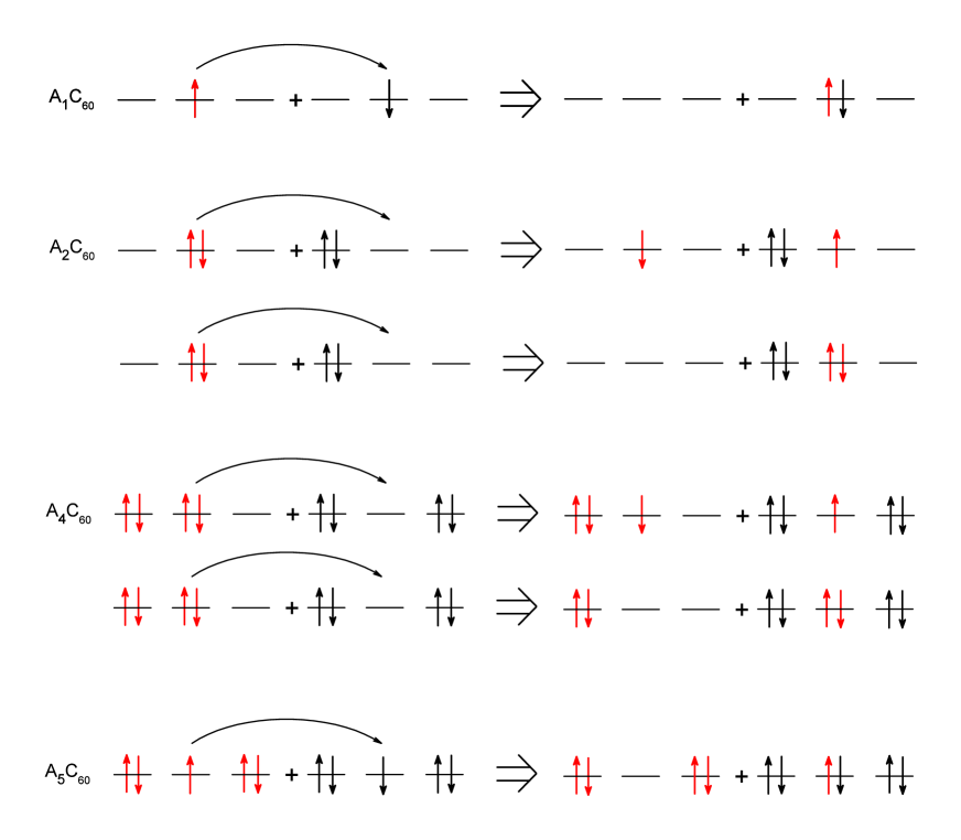
Figure 9: The charge transfer in materials $\texttt{A}_{n}\texttt{C}_{60}$ ($n=1,2,4,5$)

Using obtained results (67,72,79), values of bandwidth $W$ and Coulomb parameters $U$, $U^{\prime}$, $J$, $V$ from Tab.1 we can calculate $T_{c}$, $T_{\texttt{MI}}$, border of the collapse of conduction band (79) and the Mott parameter $\frac{\Delta E}{W}$ with $\Delta E$ from Eqs.(39,41) for $\texttt{A}_{3}\texttt{C}_{60}$ (where $\texttt{A}=\texttt{K},\texttt{Rb},\texttt{Cs}$ and the substance with cesium is considered at normal pressure, $2\texttt{kbar}$ and $7\texttt{kbar}$ with fcc structure). However we must know parameters $\lambda_{\nu}$ it order to calculate the el.-el. coupling via vibrons $\widetilde{U}_{vib}$ - Eqs.(33,34). We can use an adjustable parameter: for $\texttt{K}_{3}\texttt{C}_{60}$ the critical temperature is $T_{c}=19\texttt{K}$, then we choose the parameter of el.-vib. coupling $\lambda$ so that the critical temperature calculated from (67) would be equal to the experimental one. For other materials we calculate the parameter $\lambda$ using Eqs.(70,71), for example

$$\lambda(\texttt{Rb})=\lambda(\texttt{K})\frac{\varepsilon(\texttt{Rb})}{\varepsilon(\texttt{K})}\Rightarrow\widetilde{U}_{vib}(\texttt{Rb})=\widetilde{U}_{vib}(\texttt{K})\frac{\varepsilon^{2}(\texttt{Rb})}{\varepsilon^{2}(\texttt{K})}.$$ (80)

Moreover we must known the vibron frequency $\omega_{0}$. In a fullerene molecule an electron interacts with $A_{g}$ and $H_{g}$ vibrational modes presented in Tab.2. Then the parameter $\widetilde{U}_{vib}$ can be calculated with a following manner:

$$\widetilde{U}_{vib}=2\lambda^{2}\sum_{M=A_{g},H_{g}}\frac{1}{\omega_{M}}\left[\coth\left(\frac{\omega_{M}}{T}\right)-\frac{T}{\omega_{M}}\right]$$ (81)

Here the coupling constants $\lambda_{\nu}$ has been replaced by effective coupling constant $\lambda$: $\sum_{\nu}\lambda^{2}_{\nu}\left[V^{(\nu)}_{mm}V^{(\nu)}_{mm}+\sum_{m^{\prime}\neq m}V^{(\nu)}_{mm^{\prime}}V^{(\nu)}_{mm^{\prime}}\right]\rightarrow\lambda^{2}$, because we use $\lambda$ as an adjustable parameter. The integral (67) can be cut off by the largest vibron energy $\omega_{0}=\omega(H_{g}(8))=0.196\texttt{eV}$, that is confirmed by numerical calculation for vibron-mediated interactions in $\texttt{Cs}_{3}\texttt{C}_{60}$ in nom4 where $\omega_{0}\approx 0.19\texttt{eV}$, or it can be cut off by the half-bandwidth $W/2$ if $2\omega_{0}>W$. Results of the calculations, neglecting thermal expansion of the lattice, are presented in Tab.(3) and Fig.8. From the table we can see that without the el.-vib. interaction we have $\frac{\Delta E}{W}>1$, hence all materials would be Mott insulators. However the el.-vib. interaction and the local pairing change the relation as $\frac{\Delta E}{W}<1$, hence these materials becomes conductors, in the same time the Coulomb correlations enlarges as the lattice constant increases. The parameter $g-\frac{2}{3}\mu_{c}$ at volume per $\texttt{C}_{60}$ $784\texttt{A}^{3}$ becomes $1$, hence material $\texttt{Cs}_{3}\texttt{C}_{60}$ at pressure $2\texttt{kbar}$ is near the border of collapse of conduction band, and at normal pressure the material is Mott-Jahn-Teller insulator. As noted above at the border of collapse the localization radius becomes equal to the average distance between electrons, thus formation of polaron of small radius occurs. Such polaron can be localized on a site by the Coulomb blockade $U$. It should be noted that since $\omega_{0}\approx W/2$ for $\texttt{Cs}_{3}\texttt{C}_{60}$ at pressure $2\texttt{kbar}$ and normal pressure, then the cutting off the integral (67) by $W/2$ instead by $\omega_{0}$ does not influence on the results significantly. From Fig.8 we can see that the calculated phase diagram of alkali-doped fullirides is quantitatively close to experimental phase diagram in Fig.1.

IV Conductivity of $\texttt{A}_{n}\texttt{C}_{60}$ with $n=1,2,4,5$

For materials $\texttt{A}_{n}\texttt{C}_{60}$, where $n=1,2,4,5$, we can suppose that the el.-el. interaction $\widetilde{U}_{vib}$ via vibrons is approximately the same for these materials and is equal to the value in $\texttt{A}_{3}\texttt{C}_{60}$ $\sim 0.4\texttt{eV}$, it is analogously for Coulomb $U,U^{\prime},V$ and exchange $J$ interactions. The charge transfer in these materials is shown in Fig.9.

• $\texttt{A}_{1}\texttt{C}_{60}$. In order to form a local pair we have to transfer an electron from a site to a nearby site containing another electron. For this it is necessary to make a positive work $U-V-\widetilde{U}_{vib}>0$. Thus formation of the pairs is energetically unfavorable, i.e. the pairs are unstable. In the same time $\frac{\Delta E}{W}=\frac{U-V-\widetilde{U}_{vib}}{W}<1$, because we create the pair on a neighboring molecule. Thus this material is a conductor due the el.-vib. interaction but it is not a superconductor.

• $\texttt{A}_{2}\texttt{C}_{60}$. Two electrons are in the paired state on a site because the energy of the state is $U-U^{\prime}+J-\widetilde{U}_{vib}<0$ (measured from the Hund’s rule state). In order to transfer an electron from a site to a site we must break a pair. In this case $\frac{\Delta E}{W}=\frac{2U^{\prime}-U-V+\widetilde{U}_{vib}}{W}>1$. Thus the transfer of a electron is blocked by Coulomb interaction and the el.-el. attraction via vibrons $\widetilde{U}_{vib}$. Then the pair is compact and it could be transferred but $\frac{\Delta E}{W}=\frac{2U^{\prime}-4V}{W}>1$. Hence this material is insulator and a molecule $\texttt{C}_{60}^{2-}$ does not have spin.

• $\texttt{A}_{4}\texttt{C}_{60}$. Like the previous material all electrons are in the paired state on a site because the energy of this state is negative. We can transfer the charge from a site to a site by transferring of an electron with breaking of the pair or by transferring of the compact pair. In these cases $\frac{\Delta E}{W}$ is $\frac{2U^{\prime}-U-V+\widetilde{U}_{vib}}{W}>1$ and $\frac{2U^{\prime}-4V}{W}>1$ accordingly. Thus this material is insulator and a molecule $\texttt{C}_{60}^{4-}$ does not have spin.

• $\texttt{A}_{5}\texttt{C}_{60}$. In order to transfer an electron from a site to a nearby site we have to spend such energy that $\frac{\Delta E}{W}=\frac{3U-2U^{\prime}-V-\widetilde{U}_{vib}}{W}<1$. This process forms the pair, but $3U-2U^{\prime}-V-\widetilde{U}_{vib}>0$ - energy of the pair is positive, hence the Cooper pairs are not stable like in $\texttt{A}_{1}\texttt{C}_{60}$. Thus this material is conductor due to the el.-vib. interaction but it is not superconductor.

As expected, since the system is particle-hole symmetric, therefore the properties for $n=1,2$ are identically with the properties for $n=5,4$ accordingly. Thus we can see the el.-vib. interaction transforms Mott insulators $\texttt{A}_{n}\texttt{C}_{60}$ with $n=1,3,5$ to conductors. However for $n=2,4$ this interaction prevents conduction and it pairs electrons on each molecules so that the molecules do not have spin.

V Results

We have considered the problem of conductivity and superconductivity of alkali-doped fullerides $\texttt{A}_{n}\texttt{C}_{60}$ ($\texttt{A}=\texttt{K},\texttt{Rb},\texttt{Cs}$, $n=1\ldots 5$) while these materials would have to be antiferromagnetic Mott insulators because the on-site Coulomb repulsion is larger than bandwidth: $U\sim 1\texttt{eV}>W\sim 0.5\texttt{eV}$, and electrons on a molecule have to be distributed over molecular orbitals according to the Hund’s rule. We have found important role of 3-fold degeneration of LUMO ($t_{1u}$ level), small hopping between neighboring molecules and the coupling of electrons to Jahn-Teller modes (vibrons). The el.-el. coupling via vibrons $U_{vib}$ cannot compete with the on-site Coulomb repulsion $U\gg U_{vib}$, but it can compete with the Hund coupling $U-U^{\prime}+3J\approx 5J\sim U_{vib}$ (where the exchange energy is much less than direct Coulomb interaction $J\ll U$). This allows to form the local pair (26) on a molecule. Formation of the local pairs radically changes conductivity of these materials: they can make $\frac{\Delta E}{W}<1$, where $\Delta E$ is the energy change at transfer of an electron from a site to nearby site, while without the el.-vib. interaction we have $\frac{\Delta E}{W}>1$ that corresponds to Mott insulator. We have shown that the el.-vib. interaction and the local pairing transform Mott insulators $\texttt{A}_{n}\texttt{C}_{60}$ with $n=1,3,5$ to conductors. However for $n=2,4$ this interaction prevents conduction and it pairs electrons on each molecules so that the molecules do not have spin. The local pair mechanism can ensure superconductivity of $\texttt{A}_{3}\texttt{C}_{60}$ which is result of interplay between the el.-el. coupling via vibrons, the Coulomb blockade on a site and the hopping between neighboring sites. It should be noted that the size of a pair is larger than average distance between electrons (between molecules) and the pair is smeared over the crystal. That is in the metallic phase the local pairs have fermionic nature. At the border of transition to Mott-Jahn-Teller insulator the bosonization of local pairs occurs due to Coulomb blockage of hopping of electron between neighboring molecules. Thus system with the local pairing can be effectively described by BCS theory. In such system we have the effective coupling constant as $g-\mu_{c}>0$ (where $g$ is determined with the el.-vib. interaction and $\mu_{c}$ is determined with the Hund coupling - Eq.(58)) unlike usual metal superconductors where $g-\mu^{*}_{c}>0$ only (where $\mu^{*}_{c}$ is a Coulomb pseudopotential with Tolmachev’s reduction).

Since $\texttt{A}_{3}\texttt{C}_{60}$ is a strongly correlated system, i.e. $U/W\sim 1$, then the equation for the critical temperature (67), unlike ordinary BCS equation, accounts inter-site Coulomb correlations by renormalization parameter (64), which is $Z=0$ at transition to Mott insulator. The correlations are amplified when the conduction band compressions and they significantly suppress the critical temperature $T_{c}$. In the same time, as the crystal lattice expands (the bandwidth $W$ decreases) the density of states in the conduction band increases as $1/W$ and the el.-vib. interaction intensifies due to weakening of the screening. As a result the depending of $T_{c}$ on the volume per a molecule has a dome shape - Figs.(7,8), unlike the theoretical phase diagram calculated by DMFT method in nom1 ; nom2 . Thus el.-vib interaction ensures conductivity and superconductivity of alkali-doped fullerides. However the effectiveness of el.-vib. interaction is decreasing as temperature rises due to a vibron propagator $\frac{2\omega_{0}}{(\pi nT)^{2}+\omega_{0}^{2}}$. Hence at some temperature $T_{\texttt{MI}}$ the criterion of transition from the metallic state to the Mott insulator state will be satisfied - Eq.(72), and the material becomes Mott insulator.

As the bandwidth decreases the collapse of the conduction band to the narrow polaron band occurs when the condition (79) is satisfied. This Holstein polaron is a statical JT deformation of the molecule, where an electron supports the deformation by own field. According to JT theorem a fullerene molecule with partially filled $t_{1u}$ orbital must be distorted due to the el.-vib. interaction and the degeneracy of electron state must be removed. In the same time the molecules are combined into a lattice and their electrons are collectivized. As the lattice expands the distortions of the molecules increase, but electrons cannot be localized because the localization radius is larger than average distance between electrons (and intermolecular distance), i.e. the electrons are collectivized. This state can be called the Jahn-Teller metal which is observed in zadik . When the localization radius becomes equal and less than the average distance between electrons, then formation of polaron of small radius occurs. The polaron narrowing of the conduction band enhances Coulomb correlations in already strongly correlated system, that must turn the alkali-doped fullerides to the Mott insulator, and the material becomes Mott-Jahn-Teller insulator. We have demonstrated that border of the collapse of conduction band vertically cuts off the SC and metallic phases (at low temperature) - Figs.(7,8), unlike the theoretical phase diagram calculated in hosh .

Thus we have three phases of $\texttt{A}_{3}\texttt{C}_{60}$ illustrated schematically in Fig.(7): superconductor, metal and MJT insulator, which are separated by lines $T_{c}$, $T_{\texttt{MI}}$ and the border of collapse of conduction band. Calculated phase diagram in Fig.8 of alkali-doped fullerides is quantitatively close to experimental phase diagram in Fig.1. We have illustrated that $\texttt{K}_{3}\texttt{C}_{60},\texttt{Rb}_{3}\texttt{C}_{60}$ are conductors (and superconductors) but $\texttt{Cs}_{3}\texttt{C}_{60}$ is MJT insulator at normal pressure, at $2\texttt{kbar}$ it is superconductor on the border with MJT insulator, and at $7\texttt{kbar}$ it is superconductor with maximal $T_{c}$. Thus we have shown that superconductivity, conductivity and insulation of alkali-doped fullerides have common nature: the local pairing due to interaction with the Jahn-Teller phonons. The proposed model does not account influence of the crystal field, therefore we consider materials only with the merohedrally disordered fcc structure unlike the ordered $\texttt{A}15$ structure where the effect of crystal field should be stronger.

- (1) R. H. Zadik, Y. Takabayashi, G. Klupp, R. H. Colman, A. Y. Ganin, A. Poto nik, P. Jegli , D. Ar on, P. Matus, K. Kamar s, Y. Kasahara, Y. Iwasa, A. N. Fitch, Y. Ohishi, G. Garbarino, K. Kato, M. J. Rosseinsky, K. Prassides , Science Advances 1, no.3, e1500059 (2015), https://doi.org/10.1126/sciadv.1500059
- (2) Gyongyi Klupp, Peter Matus, Katalin Kamaras, Alexey Y. Ganin, Alec McLennan, Matthew J. Rosseinsky, Yasuhiro Takabayashi, Martin T. McDonald, Kosmas Prassides, Nature communications 3, 912 (2012), https://doi.org/10.1038/ncomms1910
- (3) Katalin Kamaras, Gyongyi Klupp, Peter Matus, Alexey Y Ganin, Alec McLennan, Matthew J Rosseinsky, Yasuhiro Takabayashi, Martin T McDonald, Kosmas Prassides, Journal of Physics: Conference Series 428, 012002 (2013), https://doi.org/10.1088/1742-6596/428/1/012002
- (4) L. Baldassarre, A. Perucchi, M. Mitrano, D. Nicoletti, C. Marini, D. Pontiroli, M. Mazzani, M. Aramini, M. Ricc, G. Giovannetti, M. Capone, S. Lupi, Scientific Reports 5, 15240 (2015), https://doi.org/10.1038/srep15240
- (5) Yasuhiro Takabayashi, Kosmas Prassides, Phil. Trans. R. Soc. A 374, 20150320 (2016), http://dx.doi.org/10.1098/rsta.2015.0320
- (6) V. Brouet, H. Alloul, Thien-Nga Le, S. Garaj, L. Forr , Phys. Rev. Lett. 86, 4680 (2001), https://doi.org/10.1103/PhysRevLett.86.4680
- (7) V. Brouet, H. Alloul, S. Garaj, L. Forro, Phys. Rev. B 66 155124 (2002), https://doi.org/10.1103/PhysRevB.66.155124
- (8) Y. Ihara, H. Alloul, P. Wzietek, D. Pontiroli, M. Mazzani, M. Ricco, Phys. Rev. Lett. 104, 256402 (2010), https://doi.org/10.1103/PhysRevLett.104.256402
- (9) Y. Ihara, H. Alloul, P. Wzietek, D. Pontiroli, M. Mazzani, M. Ricco, EPL 94, 37007 (2011), https://doi.org/10.1209/0295-5075/94/37007
- (10) H. Alloul, P. Wzietek, T. Mito, D. Pontiroli, M. Aramini, M. Ricco, J.P. Itie, E. Elkaim, Phys. Rev. Lett. 118, 237601 (2017), https://doi.org/10.1103/PhysRevLett.118.237601
- (11) O. Gunnarsson, Rev. Mod. Phys. 69, 575 (1997), https://doi.org/10.1103/RevModPhys.69.575
- (12) Guanhua Chen, William A. Goddard III, Proc. Natl. Acad. Sci. USA 90, 1350 (1993), https://doi.org/10.1073/pnas.90.4.1350
- (13) E. Cappelluti, C. Grimaldi, L. Pietronero, S. Strässler, G.A. Ummarino, Eur. Phys. J. B 21 383 (2001), https://doi.org/10.1007/PL00011123
- (14) J.E. Han, O. Gunnarsson, Physica B 292, 196 (2000), https://doi.org/10.1016/S0921-4526(00)00482-8
- (15) J.E. Han, O. Gunnarsson, V.H. Crespi, Phys. Rev. Lett. 90, 167006 (2003), https://doi.org/10.1103/PhysRevLett.90.167006
- (16) Paul E. Lammert and Daniel S. Rokhsar, Phys. Rev. B 48, 4103 (1993), https://doi.org/10.1103/PhysRevB.48.4103
- (17) D. M. Deaven, P. E. Lammert, D. S. Rokhsar, Phys. Rev. B 52, 16377 (1995), https://doi.org/10.1103/PhysRevB.52.16377
- (18) Akihisa Koga and Philipp Werner, Phys.Rev.B 91, 085108 (2015), https://doi.org/10.1103/PhysRevB.91.085108
- (19) Shugo Suzuki, Kenji Nakao, Phys. Rev. B 52, 14206 (1995), https://doi.org/10.1103/PhysRevB.52.14206
- (20) Olle Gunnarsson, Erik Koch, Richard M. Martin, Phys. Rev. B 54, R11026 (1996), https://doi.org/10.1103/PhysRevB.54.R11026
- (21) Erik Koch, The doped Fullerenes. A family of strongly correlated systems, Max-Planck-Institut für Festkörperforschung, Stuttgart, 2003
- (22) Yusuke Nomura, Shiro Sakai, Massimo Capone, Ryotaro Arita, Science Advances 1, e1500568 (2015), https://doi.org/10.1126/sciadv.1500568
- (23) Yusuke Nomura, Shiro Sakai, Massimo Capone, Ryotaro Arita, J. Phys.: Condens. Matter 28, 153001 (2016), https://doi.org/10.1088/0953-8984/28/15/153001
- (24) Shintaro Hoshino, Philipp Werner, Phys. Rev. Lett. 118, 177002 (2017), https://doi.org/10.1103/PhysRevLett.118.177002
- (25) Michael R. Savina, Lawrence L. Lohr, Anthony H. Francis, Chem. Phys. Lett. 205, 200 (1993), https://doi.org/10.1016/0009-2614(93)89230-F
- (26) F. Allonso-Marroquin, J. Giraldo, A. Calles, J.J. Castro, Rev. Mex. Fis. S 44(3), 18 (1998)
- (27) R.C. Haddon, Acc. Chem. Res. 25, 127 (1992), https://doi.org/10.1021/ar00015a005
- (28) Antoine Georges, Luca de Medici, Jernej Mravlje, Annual Reviews of Condensed Matter Physics 4, 137 (2013), https://doi.org/10.1146/annurev-conmatphys-020911-125045
- (29) Qingguo Feng, P.M. Oppeneer, Phys. Rev. B 86, 035107 (2012), https://doi.org/10.1103/PhysRevB.86.035107
- (30) Nomura Y., Nakamura K., Arita R., Phys. Rev. B 85, 155452 (2012), https://doi.org/10.1103/PhysRevB.85.155452
- (31) Olle Gunnarsson, Alkali-Doped Fullerides Narrow-Band Solids with Unusual Properties, World Scientific Publishing Co. Pte. Ltd., 2004, https://doi.org/10.1142/9789812794956
- (32) Hori C., Takada Y., Polarons and Bipolarons in Jahn Teller Crystals, Springer Series in Chemical Physics, vol 97., pp.841-871, Springer, Berlin, Heidelberg (2009), https://doi.org/10.1007/978-3-642-03432-9
- (33) V.L. Ginzburg, D.A. Kirzhnits, High-temperature superconductivity, Consultants Bureau, New York and London, 1982
- (34) Yusuke Nomura, Ryotaro Arita, Phys. Rev. B 92, 245108 (2015), https://doi.org/10.1103/PhysRevB.92.245108
- (35) Florian Gebhard, The Mott Metal-Insulator Transition. Models and Methods, Springer-Verlag Berlin Heidelberg, 1997, https://doi.org/10.1007/3-540-14858-2
- (36) J.J. Rodríguez-Núñez, A.A.Schmidt, Physica C: Superconductivity 350, 88 (2001), https://doi.org/10.1016/S0921-4534(00)01544-6
- (37) S. Dzhumanov, E.X. Karimboev, Sh.S. Djumanov, Phys. Lett. A 380, 2173 (2016), https://doi.org/10.1016/j.physleta.2016.04.038
- (38) G. Litak, T. Örd, K. Rägo and A. Vargunin, Acta Physica Polonica A 121, 747 (2012), https://doi.org/10.12693/APhysPolA.121.747
- (39) I.N. Askerzade, Physica C 397, 99 (2003), https://doi.org/10.1016/j.physc.2003.07.003
- (40) I.N. Askerzade, Physics-Uspekhi 49, 1003 (2006), https://doi.org/10.1070/PU2006v049n10ABEH006055
- (41) I.N. Askerzade, J. Phys. Chem. Solids 68, 1311 (2007), https://doi.org/10.1016/j.jpcs.2007.02.016
- (42) Konstantin V. Grigorishin, Phys. Lett. A 380, 1781 (2016), https://doi.org/10.1016/j.physleta.2016.03.023
- (43) V.M. Loktev, S.G. Sharapov, Cond. Matter Physics (Lviv) No.11., 131 (1997), http://dx.doi.org/10.5488/CMP.11.131
- (44) William Jones, Norman H. March, Theoreoretical solid state physics, Vol.2, Dover Publications, Inc., New York, 1985.
- (45) W.F. Brinkman, T.M. Rice, Phys. Rev. B 2, 4302 (1970), https://doi.org/10.1103/PhysRevB.2.4302
- (46) R. Bulla, T.A. Costi, Vollhardt D., Phys.Rev.B 64, 045103 (2001), https://doi.org/10.1103/PhysRevB.64.045103
- (47) M.S. Golden, M. Knupfer, J. Fink, J.F. Armbruster, T.R. Cummins, H.A. Romberg, M. Roth, M. Sing, M. Schmidt, E. Sohmen, J. Phys.: Cond. Matter 7, 8219 (1995), https://doi.org/10.1088/0953-8984/7/43/004
- (48) Ping Zhou, Kai-An Wang, A.M. Rao, P.C. Eklund, G. Dresselhaus, M.S. Dresselhaus, Phys. Rev. B 45, 10838(R) (1992), https://doi.org/10.1103/PhysRevB.45.10838
- (49) S. Dzhumanov, U.T. Kurbanov, Z.S. Khudayberdiev, A. R. Hafizov, Low Temp. Phys 42(11), 1057 (2016), http://dx.doi.org/10.1063/1.4971169
- (50) A.S. Alexandrov, A.B. Krebs, Sov. Phys. Usp. 35, 345 (1992), https://doi.org/10.1070/PU1992v035n05ABEH002235
- (51) M. Casula, Ph. Werner, L. Vaugier, F. Aryasetiawan, T. Miyake, A. J. Millis, S. Biermann, Phys. Rev. Lett. 109, 126408 (2012), https://doi.org/10.1103/PhysRevLett.109.126408
- (52) Yuta Murakami, Philipp Werner, Naoto Tsuji, Hideo Aok, Phys. Rev. B 88, 125126 (2013), https://doi.org/10.1103/PhysRevB.88.125126
- (53) A.S. Alexandrov, Phys. Rev. B 61, 12315 (2000), https://doi.org/10.1103/PhysRevB.61.12315
- (54) S.Wehrli, M. Sigrist, Phys. Rev. B 76, 125419 (2007), https://doi.org/10.1103/PhysRevB.76.125419
- (55) David R. Penn, Phys. Rev. 142, 350 (1966), https://doi.org/10.1103/PhysRev.142.350
- (56) Yu. A. Izyumov, Sov. Phys. Usp. 38, 385 (1995), http://dx.doi.org/10.1070/PU1995v038n04ABEH000081