Stability band structure for periodic states in periodic potentials

Abstract

A class of periodic solutions of the nonlinear Schrödinger equation with non-Hermitian potentials are considered. The system may be implemented in planar nonlinear optical waveguides carrying an appropriate distribution of local gain and loss, in a combination with a photonic-crystal structure. The complex potential is built as a solution of the inverse problem, which predicts the potential supporting required periodic solutions. The main subject of the analysis is the spectral structure of the linear (in)stability for the stationary spatially periodic states in the periodic potentials. The stability and instability bands are calculated by means of the plane-wave-expansion method, and verified in direct simulations of the perturbed evolution. The results show that the periodic solutions may be stable against perturbations in specific Floquet-Bloch bands, even if they are unstable against small random perturbations.

1 Introduction

Non-Hermitian (complex) potentials in wave equations give rise to effects that cannot be realized with Hermitian (real) potentials, well-known examples being the parity-time ($\mathcal{PT}$) symmetry in the case when the real and imaginary parts of the complex potential are, respectively, spatially even and odd [1, 2, 3, 4]. The $\mathcal{PT}$ symmetry, i.e., the reality of the energy spectrum in the respective systems, holds up to a critical value of the strength of the imaginary potential, symmetry breaking occurring above the critical value. In optics, $\mathcal{PT}$-symmetric potentials have been realized in various experiments [5, 6, 7, 8, 9, 10, 11, 12]. They exhibit remarkable properties and potential applications, such as power oscillations [6], non-reciprocal light propagation [13], optical transparency [14], negative refraction [15], pseudo-Hermitian Bloch oscillations [16, 17], unidirectional invisibility [18, 19, 20], and possibilities to design various $\mathcal{PT}$-symmetric devices [21, 23, 22, 24], as recently reviewed in Ref. [25]. Further, optics provides a fertile ground to investigate $\mathcal{PT}$-symmetric beam dynamics in nonlinear regimes, including the formation of bright and dark solitons, gap solitons, defect states, multi-peak modes, and vortices, see original works [26, 27, 28, 29, 30, 31, 32, 33, 34, 35, 36, 37, 38, 39, 40, 41, 42, 43, 44, 45, 46, 47, 48] and recent reviews [49, 50]. In particular, a specific arrangement of the self-defocusing nonlinearity, growing from the center to periphery, makes it possible to predict self-trapped modes featuring unbreakable $\mathcal{PT}$ symmetry [51]. The concept of the $\mathcal{PT}$-symmetry has also been applied to Bose-Einstein condensates [52, 53, 54, 55], atomic cells [56, 57, 58], and nonlinearity-induced $\mathcal{PT}$-symmetry without material gain [59].

Stability of optical solitons and nonlinear beam dynamics in non-$\mathcal{PT}$-symmetric complex potentials was also addressed, showing that the solitons may be stable in a wide range of parameters [61, 60, 62, 63, 49]. Some applications, such as coherent perfect absorbers and time-reversal lasers, have been elaborated in such settings [64, 65, 66, 67, 68], and non-$\mathcal{PT}$-symmetric optical potentials with all-real spectra in a coherent atomic system have been realized [69]. The studies of the stability of modes supported by the complex potentials make this topic a part of the very broad field of dynamical stability in various nonlinear systems. One of basic problems in this field is the modulation instability (MI) of extended states.

In particular, the MI was widely studied in $\mathcal{PT}$-symmetric nonlinear Schrödinger (NLS) equations [70, 71, 72, 73, 74, 75, 76]. Recently, the MI of constant-amplitude waves has been addressed in models with more general complex potentials by using the plane-wave-expansion method combined with direct simulations [77, 78], which makes it possible to calculate the stability band structure of spatially periodic solutions in periodic complex potentials. In the present work, we aim to explore this structure for periodic solutions of the NLS equation with non-Hermitian potentials.

The paper is organized as follows. In the next section, the model and its reduction are introduced, and the corresponding periodic solutions are presented by solving an inverse problem, which predicts the periodic potentials supporting a required phase-gradient structure of the periodic solutions. In Sec. III, we focus on the analysis of the stability band structure of the periodic solutions, employing the plane-wave-expansion method. The conclusions are made in Sec. IV.

2 Model and periodic solutions

We begin the analysis by considering the NLS equation with non-Hermitian potentials, written in a scaled form, cf. Ref. [77]:

$$i\frac{\partial\Psi}{\partial z}+\frac{\partial^{2}\Psi}{\partial x^{2}}+V(x)\Psi+g\left|\Psi\right|^{2}\Psi=0.$$ (1)

In the application to light propagation in planar waveguides, $\Psi(x,z)$ is the slowly varying envelope of the electric field, $z$ and $x$ are the propagation distance and the transverse coordinate,

$$V(x)\equiv V_{R}(x)+iV_{I}(x)$$ (2)

is the complex potential, which can be implemented in optics by combining the spatially modulated refractive index and spatially distributed gain and loss elements [6]. The nonlinearity can be either self-focusing ($g>0$) or defocusing ($g<0)$, the latter being possible in semiconductor optical materials [79]. We are looking for stationary solutions of Eq. (1) as

$$\Psi(x,z)=\Phi(x)\exp(i\mu z),$$ (3)

where $\mu$ is a real propagation constant and complex field profile $\Phi(x)$ is determined by the following nonlinear equation:

$$-\mu\Phi+\Phi^{{}^{\prime\prime}}+V(x)\Phi+g\left|\Phi\right|^{2}\Phi=0,$$ (4)

with the prime standing for $d/dx$. Further, we define real amplitude and phase

$$\Phi(x)=H\left(x\right)\exp\left[i\Theta(x)\right],$$ (5)

for which complex Eq. (4) splits into real ones:

$$-\mu H+H^{{}^{\prime\prime}}-H(\Theta^{{}^{\prime}})^{2}+V_{R}H+gH^{3} =0,$$ (6)

$$2H^{{}^{\prime}}\Theta^{\prime}+H\Theta^{{}^{\prime\prime}}+V_{I}H =0.$$ (7)

Equations (6) and (7) may be addressed as an inverse problem, which provides a required form of the solution, $H(x)$ and $\Theta(x)$, by selecting a particular complex potential (2):

$$V_{R}\left(x\right) =\mu-\frac{H^{{}^{\prime\prime}}}{H}+(\Theta^{{}^{\prime}})^{2}-gH^{2},$$ (8)

$$V_{I}\left(x\right) =-2\frac{H^{{}^{\prime}}\Theta^{\prime}}{H}-\Theta^{{}^{\prime\prime}}.$$ (9)

The approach based on the inverse problem was previously elaborated in various contexts related to NLS equations [80, 81, 82, 83, 84].

To choose basic periodic solutions to Eq. (1), avoiding singularities in the complex potential, we set $H^{{}^{\prime\prime}}/H=-\omega^{2}$ and $\Theta^{\prime}=V_{0}H$, where $\omega$ and $V_{0}$ are the real constants. Accordingly, we have

$$H(x) =A\sin(\omega x+\phi),$$ (10)

$$\Theta(x) =-\frac{V_{0}A}{\omega}\cos\left(\omega x+\phi\right),$$ (11)

with arbitrary real constants $A$ and $\phi$. Thus, the starting point is the periodic solution of Eq. (1) taken as

$$\Psi(x,z)=H\left(x\right)e^{i\Xi(x,z)},$$ (12)

$$\Xi(x,z)\equiv\mu z-\frac{AV_{0}}{\omega}\cos(\omega x+\phi),$$

with the corresponding real and imaginary parts of the complex potential given by Eqs. (8) and (9):

$$V_{R}\left(x\right) =\mu+\omega^{2}+\left(V_{0}^{2}-g\right)H^{2}\left(x\right),$$ (13)

$$V_{I}\left(x\right) =-3V_{0}H^{\prime}\left(x\right).$$ (14)

The complex periodic potential $V\left(x\right)$ given by Eqs. (13) and (14) is similar to the so-called Wadati potential [85], with even and odd real and imaginary parts, respectively. Note that the periodic solution exists in the linear limit ($g=0$), as well as for an arbitrary strength of the nonlinearity ($g\neq 0$). Lastly, function $H\left(x\right)$ determines the power flow from gain to loss regions, the respective Poynting vector, $S=(i/2)(\Psi\partial\Psi^{\ast}/\partial x-\Psi^{\ast}\partial\Psi/\partial x)$, taking a very simple form, $S=V_{0}H^{3}$, proportional to the gain-loss strength, $V_{0}$.

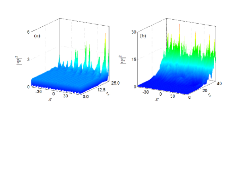
Figure 1: (Color online) The evolution of the perturbed periodic solution under the action of the periodic complex potential $V(x)$ given by Eqs. (13) and (14) for (a) the self-focusing nonlinearity with $g=0.3$ and $V_{0}=0.23$; and (b) the defoucsing nonlinearity with $g=-0.7$ and $V_{0}=0.2$. Here, the perturbation amplitude $\varepsilon=0.02$, and the other parameters are taken as $A=1$, $\omega=1$, $\phi=\pi/2$, and $\mu=-1$.

3 The stability-band structure of the periodic solution

In this section, we address the stability of the periodic solution (12), using the plane-wave-expansion method for the linear-stability analysis. The results will be verified by means of direct numerical simulations.

The linear-stability analysis is initiated by adding a small perturbation to periodic solution (12):

$$\Psi(x,z)=\left[H+\varepsilon F_{\lambda}(x)e^{i\lambda z}+\varepsilon G_{\lambda}^{\ast}(x)e^{-i\lambda^{\ast}z}\right]e^{i\Xi(x,z)},$$ (15)

where $\ast$ stands for the complex conjugate, and $\varepsilon$ is a real infinitesimal amplitude of the perturbation with complex eigenfunctions $F_{\lambda}\left(x\right)$ and $G_{\lambda}\left(x\right)$, which are related to complex eigenvalue $\lambda$. As usual, an imaginary part of $\lambda$, if any, defines the instability growth rate of the perturbation. The substitution of expression (15) into Eq. (1) and subsequent linearization leads to the eigenvalue problem in the matrix form,

$$\left(\begin{array}[c]{cc}L_{1}&gH^{2}\\ -gH^{2}&L_{2}\end{array}\right)\left(\begin{array}[c]{c}F_{\lambda}\left(x\right)\\ G_{\lambda}\left(x\right)\end{array}\right)=\lambda\left(\begin{array}[c]{c}F_{\lambda}\left(x\right)\\ G_{\lambda}\left(x\right)\end{array}\right),$$ (16)

where the operators $L_{1}$ and $L_{2}$ are

$$L_{1} =-\mu+gH^{2}-2iV_{0}H_{x}+2iV_{0}H\partial_{x}+\partial_{xx},$$ (17)

$$L_{2} =\mu-gH^{2}-2iV_{0}H_{x}+2iV_{0}H\partial_{x}-\partial_{xx}.$$ (18)

The linear eigenvalue problem (16) can be solved by the finite difference method. As typical examples, we calculated the eigenvalues of Eq. (16), finding that the instability growth rates are $0.0036$ and $0.5673$ for parameters given in the caption to Fig. 1, for the self-focusing and defocusing nonlinearity, respectively, which means that the periodic solution (12) is unstable. To confirm the results, we have performed simulations of the evolution of solution (12) with random-noise perturbations added to it, as shown in Figs. 1(a) and 1(b).

The above results do not include the stability band structure of the periodic solution (12). Below, we will apply the plane-wave-expansion method based on Eq. (16) [77] to produce the band structure. In the framework of this method in its general form, because $H(x)$ is a periodic function with period of $2\pi/\omega$, the perturbation eigenmodes $F_{\lambda}\left(x\right)$ and $G_{\lambda}\left(x\right)$, along with $H(x)$ itself, are expanded into Fourier series, according to the Floquet-Bloch theorem:

$$\left(\begin{array}[c]{c}F_{\lambda}\left(x\right)\\ G_{\lambda}\left(x\right)\end{array}\right) ={\displaystyle\sum_{n=-\infty}^{+\infty}}\left(\begin{array}[c]{c}u_{n}(k)\\ v_{n}(k)\end{array}\right)e^{i(n\omega+k)x},$$ (23)

$$H(x) ={\displaystyle\sum_{n=-\infty}^{+\infty}}H_{n}e^{in\omega x},$$ (24)

where $k$ is the Bloch momentum, making the eigenmodes quasiperiodic functions of $x$. Substituting Eqs. (13), (14), (23) and (24) into the eigenvalue problem (16), one arrives at the following system of linear equations for perturbation coefficients $u_{n}$, $v_{n}$ and eigenvalue $\lambda(k)$:

$$\lambda(k)u_{n} =\delta u_{n-2}+\delta v_{n-2}+\beta_{n-1}u_{n-1}$$

$$+\alpha_{n}u_{n}+\gamma_{n+1}u_{n+1}+\sigma u_{n+2}+\sigma v_{n+2},$$

$$\lambda(k)v_{n} =-\delta u_{n-2}-\delta v_{n-2}+\beta_{n-1}v_{n-1}$$

$$-\alpha_{n}v_{n}+\gamma_{n+1}v_{n+1}-\sigma u_{n+2}-\sigma v_{n+2},$$ (25)

where we define

$$\delta =-\frac{1}{4}gA^{2}e^{i2\phi},$$ (26)

$$\sigma =-\frac{1}{4}gA^{2}e^{-i2\phi},$$ (27)

$$\alpha_{n} =-\mu-(n\omega+k)^{2},$$ (28)

$$\beta_{n} =-iAV_{0}[\left(n+1\right)\omega+k]e^{-i\phi},$$ (29)

$$\gamma_{n} =iAV_{0}[\left(n-1\right)\omega+k]e^{i\phi}.$$ (30)

The instability growth rate of the periodic solution is again defined as the largest imaginary part of $\lambda(k)$, in the set of the eigenvalues for given $k$. As a typical example, Fig. 2 depicts the dependence of $\max[\operatorname{Im}\lambda(k)]$ on $k$ (in the half of the first Brillouin zone) for different values of the gain/loss parameter $V_{0}$ in both the self-focusing and defocusing regimes.

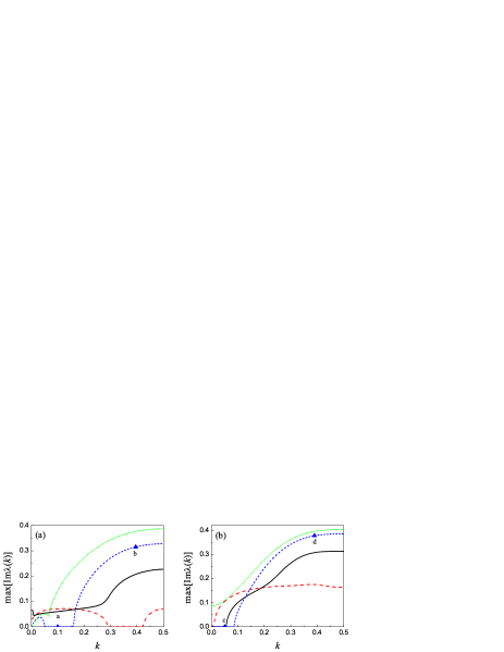
Figure 2: (Color online) The dependence of the instability growth rate, i.e., the largest imaginary part of eigenvalues $\lambda(k)$, on the Bloch wavenumber $k$ (in the half of the first Brillouin zone) for different values of the gain/loss coefficient $V_{0}$. Panels (a) and (b) report the results of the self-focusing ($g=0.3$) and defocusing ($g=-0.7$) nonlinearity, respectively. Red dashed, black solid, blue short-dashed, and green short-dotted curves correspond to $V_{0}=$ $0.05$, $0.16$, $0.23$, and $0.27$ in (a), and $V_{0}=0.08$, $0.16$, $0.20$, and $0.21$ in (b), respectively. Other parameters are the same as in Fig. 1.

For the self-focusing nonlinearity, as seen in Fig. 2(a), at $V_{0}=0.16$ and $V_{0}=0.27$ the eigenvalues with the largest imaginary part are complex at all $k$ [see the black solid and green short-dotted curves in Fig. 2(a)], hence the periodic solution is linearly unstable to all perturbations. When $V_{0}=0.05$ and $0.23$, as shown by the red dashed and blue short-dashed curves in Fig. 2(a), a stability band, i.e., an interval of wavenumber $k$ in which the instability growth rate vanishes, can be formed. This means that the periodic solution is stable against perturbations corresponding to the Floquet-Bloch modes in intervals $k\in[0.29,0.42]$ as $V_{0}=0.05$, and $[0.055,0.155]$ as $V_{0}=0.23$, respectively.

Similarly, for the defocusing nonlinearity, as shown in Fig. 2(b), at $V_{0}=0.08$ and $V_{0}=0.21$, the eigenvalues with the largest imaginary part are complex at all $k$ [see the red dashed and green short dotted curves in Fig. 2(b)]. On the other hand, at $V_{0}=0.16$ and $0.2$ stability bands are $[0,0.055]$ and $[0,0.085]$, respectively. They are narrower than the instability zone, and are mainly located near the center of the Brillouin zone [see the black solid and blue short-dashed curves in Fig. 2(b)].

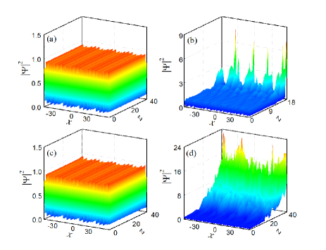
Figure 3: (Color online) The simulated evolution of the periodic solution, perturbed by specific eigenmodes (see the text), under the action of the self-focusing nonlinearity ($g=0.3$) and periodic potential ($V_{0}=0.23$) in (a) and (b), and defocusing nonlinearity ($g=-0.7$) and periodic potential ($V_{0}=0.2$) in (c) and (d). Here, (a) $k=0.1$; (b) $k=0.39$; (c) $k=0.05$, and (d) $k=0.39$. The perturbation amplitude is $\varepsilon=0.02$, and other parameters are the same as in Fig. 1.

To verify the above results, we have performed systematic simulations of Eq. (1) by taking inputs in the form of the periodic solution with the addition of small perturbations corresponding to specific Floquet-Bloch eigenmodes, as per Eq. (15). Figs. 3(a) and 3(b) show the evolution of the periodic solution perturbed by the eigenmodes corresponding to $k=0.1$ and $k=0.39$ at $V_{0}=0.23$ in the self-focusing regime. As predicted by points “a” and “b” in Fig. 2(a), the periodic solution is stable against these perturbation modes at $k=0.1$ [Fig. 3(a)], and unstable at $k=0.39$ [Fig. 3(b)]. Figs. 3(c) and 3(d) display the evolution in the system with $V_{0}=0.2$ and the defocusing nonlinearity, where the perturbation eigenmodes corresponding to $k=0.05$ and $k=0.39$ are initially added, respectively. They demonstrate that, in agreement with the prediction of points “c” and “d” in Fig. 2(b), the periodic solution is stable to the perturbations at $k=0.05$, see Fig. 3(c), and it is unstable to $k=0.39$, as shown in Fig. 3(d).

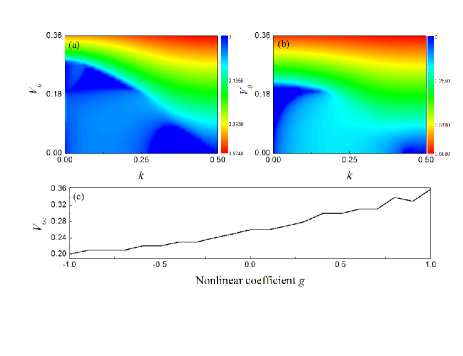
Figure 4: (Color online) The dependence of the largest imaginary part of the eigenvalues on $V_{0}$ in the half of first Brillouin zone for (a) $g=0.3$ and (b) $g=-0.7$, respectively. (c) The critical value $V_{0c}$, beyond which the stability band does not exist at all $k$, versus the nonlinearity coefficient $g$. Other parameters are the same as in Fig. 1.

To exhibit the influence of the gain/loss parameter $V_{0}$ on the stability band structure, Fig. 4 presents the largest imaginary part of the eigenvalues vs. $V_{0}$ in the half of first Brillouin zone for both the self-focusing and defocusing nonlinearities. For the self-focusing case, as shown in Fig. 4(a), the stability band does not exist at all $k$ when $V_{0}$ belongs to intervals $0.08<V_{0}<0.2$ and $0.26<V_{0}<0.36$, while in intervals $0\leq V_{0}\leq 0.08$ and $0.2\leq V_{0}\leq 0.26$ the stability band appears in some interval of $k$, which shrinks with the increase of $V_{0}$. Fig. 4(b) shows the defocusing case. Similarly, we find that the stability band does not exist at all $k$ when $V_{0}\in(0.02,0.08)\cup(0.20,0.36)$, while in $[0.08,0.20]$ the stability band appears in some interval of $k$, chiefly near the center of the Brillouin zone. For the self-focusing or defocusing nonlinearity alike, there exists a critical value $V_{0c}$ such that, at $V_{0}>V_{0c}$, stability banks do not exist. Fig. 4(c) presents the dependence of critical value $V_{0c}$ on the nonlinearity coefficient, $g$. Naturally, $V_{0c}$ increases with $g$, as the interplay of the nonlinearity with the $\mathcal{PT}$ symmetry usually accelerates the onset of the breakup of the symmetry.

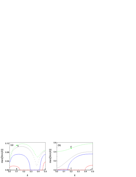
Figure 5: (Color online) The dependence of the instability growth rate, $\max[\operatorname{Im}\lambda(k)]$, on Bloch wavenumber $k$ (in the half of the first Brillouin zone) for different values of the amplitude $A$ of the stationary periodic solution. Panels (a) and (b) present the results for the self-focusing ($g=0.3$) and defocusing ($g=-0.7$) nonlinearity, respectively. Black solid, red short-dashed, blue short-dotted, gray circled, and green dotted curves correspond to $A=0.1$, $0.5$, $1.0$, $1.23$, and $1.3$ in (a), and $A=0.1$, $0.35$, $0.95$, $1.03$, and $1.3$ in (b). The strength of the gain-loss term is $V_{0}=0.05$ in (a) and $V_{0}=0.2$ in (b), respectively, other parameters being $\omega=1$, $\phi=\pi/2$, and $\mu=-1$.

In contrast with the results displayed in Fig. 1, even if the periodic solution is unstable against small random-noise perturbations, it may be effectively stable against perturbations in the form of specific Floquet-Bloch eigenmodes, due to the existence of the respective stability band, as shown in Figs. 3(a,c), which we call band stability.

Next, Fig. 5 shows the effect of amplitude $A$ of the stationary periodic solution on its stability. For the self-focusing nonlinearity, as seen in Fig. 5(a), at $A=1.23$ and $A=1.3$ [the gray circled and green dotted curves in Fig. 5(a)] the periodic solutions are unstable to perturbations with all values of $k$. At $A=0.1$, $0.5$ and $1.0$ [see black solid, red short-dashed, and blue short-dotted curves in Fig. 5(a)], stability bands are the intervals of $k\in[0,0.49]$, $[0.15,0.46]$, and $[0.29,0.42]$, respectively, whose widths shrink with the increasing of $A$.

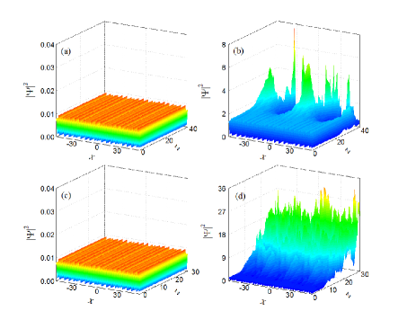
Figure 6: (Color online) The simulated evolution of periodic solutions, perturbed by specially selected eigenmodes (see the text), under the action of the self-focusing nonlinearity ($g=0.3$) in (a) and (b), and defocusing nonlinearity ($g=-0.7$) in (c) and (d). The parameters are: (a) $A=0.1$, $V_{0}=0.05$, $k=0.1$; (b) $A=1.3$, $V_{0}=0.05$, $k=0.1$; (c) $A=0.1$, $V_{0}=0.2$, $k=0.2$; (d) $A=1.3$, $V_{0}=0.2$, $k=0.2$. The perturbation amplitude is $\epsilon=0.01$, other parameters being the same as in Fig. 5.

Similarly, for the defocusing nonlinearity, as seen in Fig. 5(b), at $A=1.03$ and $A=1.3$ the stationary periodic solutions are again unstable to perturbations with all $k$, see the gray circled and green dotted curves in Fig. 5(b). At $A=0.1$, $0.35$, and $0.95$, as shown by the black solid, red short-dashed, and blue short-dashed curves in Fig. 5(b), the stability bands are the intervals of $k\in[0.05,0.46]$, $[0.19,0.39]$, and $[0,0.15]$, respectively.

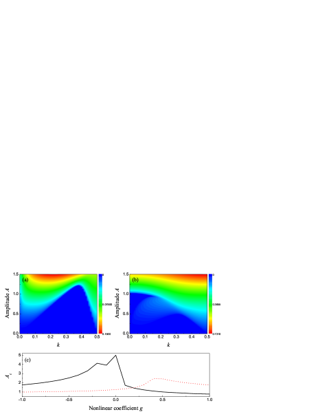
Figure 7: (Color online) The dependence of the instability growth rate, i.e., the largest imaginary part of the eigenvalues, on amplitude $A$ of the stationary solutions in the half of first Brillouin zone, for (a) $g=0.3$, $V_{0}=0.05$, and (b) $g=-0.7$, $V_{0}=0.2$. (c) The critical value $A_{c}$, beyond which the instability occurs at all $k$, versus the nonlinearity coefficient, $g$. Other parameters are the same as in Fig. 5.

The above results can be confirmed by simulations of Eq. (1) with inputs in the form of the periodic solution with the addition of small perturbations corresponding to specific Floquet-Bloch eigenmodes. Figs. 6(a) and 6(b) show the evolution of the periodic solutions perturbed by the eigenmodes with $k=0.1$ for $A=0.1$ and $A=1.3$, with the gain/loss coefficient $V_{0}=0.05$, in the self-focusing regime. As predicted by points “a” and “b” in Fig. 5(a), the periodic solution is stable for $A=0.1$ [Fig. 6(a)], and unstable for $A=1.3$ [Fig. 6(b)]. Figs. 6(c) and 6(d) display the corresponding results in the defocusing regime, where the perturbation eigenmodes with $k=0.2$ for $A=0.1$ and $A=1.3$ are initially added to the system with $V_{0}=0.2$. It is seen that the periodic solution is stable at $A=0.1$, see Fig. 6(c), and it is unstable at $A=1.3$, see Fig. 6(d), in agreement with the predictions produced by points “c” and “d” in Fig. 5(b).

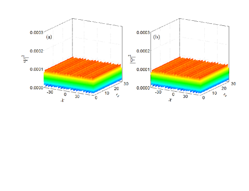
Figure 8: (Color online) The evolution of the perturbed periodic solution under the action of the periodic complex potential $V(x)$ given by Eqs. (13) and (14) for (a) the self-focusing nonlinearity with $g=0.3$ and $V_{0}=0.05$; and (b) the defoucsing nonlinearity with $g=-0.7$ and $V_{0}=0.2$. Here, the perturbation amplitude $\varepsilon=0.02$, and the other parameters are taken as $A=0.01$, $\omega=1$, $\phi=\pi/2$, and $\mu=-1$.

Further, Fig. 7 shows the dependence of the largest imaginary part of the eigenvalues on amplitude $A$ of the stationary periodic solutions in the half of first Brillouin zone for the self-focusing and defocusing nonlinearities. In the former case, Fig. 7(a) shows that the eigenvalues are almost completely real at all $k$ for small $A$. With the increase of $A$, the stability band shrinks up to $A=1.23$, beyond which the eigenvalues with the largest imaginary part are complex at all $k$. Similarly, in the defocusing regime, the periodic solutions are stable at all $k$ for small $A$, and the instability takes place at all values of $k$ for $A>1.03$, as shown in Fig. 7(b). The dependence of the critical value $A_{c}$, beyond which the instability occurs at all $k$, on the nonlinearity coefficient $g$ is presented in Fig. 7(c), for $V_{0}=0.05$ and $0.2$ (the black solid and red dotted curves), respectively. In particular, in the former case, the dependence $A_{c}(g)$  clearly implies that the instability is essentially stronger for the self-focusing sign of the nonlinearity ($g>0$), which is quite natural, as the self-focusing pushes the system towards the breakup of the $\mathcal{PT}$ symmetry by imposing the modulational instability.

As the result, the periodic solutions are stable at all wavenumber $k$ for small $A$. In this case, we conclude that they will be stable against small random-noise perturbations, i.e., dynamical stable. A lot of numerical simulations confirm the conclusion. As the typical example, Fig. 8 exhibits the stable evolution of the periodic solutions for $A=0.01$, $g=0.3$, $V_{0}=0.05$ and $A=0.01$, $g=-0.7$, $V_{0}=0.2$, respectively, which the instability growth rate is $0$ for all $k$, as shown in Figs. 7(a) and 7(b).

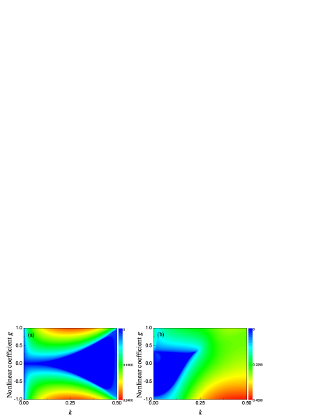
Figure 9: (Color online) The dependence of the instability growth rate, $\max[\operatorname{Im}\lambda(k)]$, on the nonlinearity coefficient, $g$, and wavenumber, $k$, for (a) $V_{0}=0.01$ and (b) $V_{0}=0.2$. Here, the parameters are $A=1$, $\omega=1$, $\phi=\pi/2$, and $\mu=-1$.

Finally, we consider the effect of the nonlinearity coefficient, $g$, on the stability band of the periodic solution. Fig. 9 displays the dependence of the instability growth rate on $g$ in the half of the first Brillouin zone for different values of the gain/loss coefficient, $V_{0}$. In Fig. 9(a), at $V_{0}=0.01$ the stability band emerges near the edge of the Brillouin zone, and its size increases with the decrease of $\left|g\right|$, reaching a maximum at $g=0$. Note that the respective contour plot is almost symmetric with respect to $g=0$. However, the symmetry is  broken at larger $V_{0}$, as seen in Fig. 9(b), which displays the corresponding results at $V_{0}=0.2$. They demonstrate, in particular, that the instability occurs at all $k$ when $g$ belongs to intervals $-1<g<-0.91$ and $0.34<g<1$. At $-0.91<g<0.34$, the stability band exists, and its size grows with the increase of $g$.

4 Conclusion

We have considered periodic solutions produced by the NLS equation with the non-Hermitian potential. The model is built with the help of the inverse-problem approach, which selects the complex periodic potential needed to support by periodic states with the simple phase-gradient structure. The setting can be realized in optical nonlinear waveguides, with an appropriate distribution of the local gain and loss. The analysis was focused on the linear-stability band structures of the periodic solutions, calculated by means of the plane-wave-expansion method. The results shows that, even if the periodic solutions are unstable against small random perturbations, they may be stable against perturbations of specific Floquet-Bloch eigenmodes, due to the presence of the stability band in the periodic potential. The approach elaborated in the present work can be used to analyze stability band structures of periodic solutions in periodic complex potentials for other nonlinear systems.

References

References

- [1] C. M. Bender and S. Boettcher, Real Spectra in Non-Hermitian Hamiltonians Having Symmetry, Phys. Rev. Lett. 80 (1998) 5243-5246.
- [2] A. Mostafazadeh, Pseudo-Hermiticity versus -symmetry III: Equivalence of pseudo-Hermiticity and the presence of antilinear symmetries, J. Math. Phys. 43 (2002) 3944-3951.
- [3] C. M. Bender, D. C. Brody, and H. F. Jones, Complex Extension of Quantum Mechanics, Phys. Rev. Lett. 89 (2002) 270401.
- [4] C. M. Bender, Making sense of non-Hermitian Hamiltonians, Rep. Prog. Phys. 70 (2007) 947-1018.
- [5] A. Guo, G. J. Salamo, D. Duchesne, R. Morandotti, M. Volatier-Ravat, V. Aimez, G. A. Siviloglou, and D. N. Christodoulides, Observation of PT-Symmetry Breaking in Complex Optical Potentials, Phys. Rev. Lett. 103 (2009) 093902.
- [6] C. E. Rüter, K. G. Makris, R. El-Ganainy, D. N. Christodoulides, M. Segev, and D. Kip, Observation of parity-time symmetry in optics, Nature Phys. 6 (2010) 192-195; T. Kottos, Broken symmetry makes light work, Nature Phys. 6 (2010) 166-167.
- [7] A. Regensburger, C. Bersch, M. -A. Miri, G. Onishchukov, D. N. Christodoulides, and U. Peschel, Parity-time synthetic photonic lattices, Nature 488 (2012) 167-171.
- [8] L. Feng, Y. -L. Xu, W. S. Fegadolli, M. -H. Lu, J. E. B. Oliveira, V. R. Almeida, Y. -F. Chen, and A. Scherer, Experimental demonstration of a unidirectional reflectionless parity-time metamaterial at optical frequencies, Nature Mater. 12 (2013) 108-113.
- [9] L. Chang, X. Jiang, S. Hua, C. Yang, J. Wen, and L. Jiang, G. Li, G. Wang, and Min Xiao, Parity-time symmetry and variable optical isolation in active-passive-coupled microresonators, Nature Phot. 8 (2014) 524-529.
- [10] B. Peng, S. Kayaözdemir, F. Lei, F. Monifi, M. Gianfreda, G. L. Long, S. Fan, F. Nori, C. M. Bender, and L. Yang, Parity-time-symmetric whispering-gallery microcavities Nature Phys. 10 (2014) 394-398.
- [11] Z. Zhang, Y. Zhang, J. Sheng, L. Yang, M.-A. Miri, D. N. Christodoulides, B. He, Y. Zhang, and M. Xiao, Observation of Parity-Time Symmetry in Optically Induced Atomic Lattices, Phys. Rev. Lett. 117 (2016) 123601.
- [12] Z. Gao, S. T. M. Fryslie, B. J. Thompson, P. S. Carney, and K. D. Choquette, Parity-time symmetry in coherently coupled vertical cavity laser arrays, Optica 4 (2017) 323-329.
- [13] K. G. Makris, R. El-Ganainy, D. N. Christodoulides, and Z. H. Musslimani, Beam Dynamics in PT Symmetric Optical Lattices, Phys. Rev. Lett. 100 (2008) 103904.
- [14] A. Guo, G. J. Salamo, D. Duchesne, R. Morandotti, M. Volatier-Ravat, V. Aimez, G. A. Siviloglou, and D. N. Christodoulides, Observation of PT-Symmetry Breaking in Complex Optical Potentials, Phys. Rev. Lett. 103 (2009) 093902.
- [15] R. Fleury, D. L. Sounas, and A. Alù, Negative Refraction and Planar Focusing Based on Parity-Time Symmetric Metasurfaces, Phys. Rev. Lett. 113 (2014) 023903.
- [16] S. Longhi, Bloch Oscillations in Complex Crystals with PT Symmetry, Phys. Rev. Lett. 103 (2009) 123601.
- [17] M. Wimmer, M. Miri, D. Christodoulides, Ulf Peschel, Observation of Bloch oscillations in complex PT-symmetric photonic lattices, Scientific Reports 5 (2015) 17760.
- [18] H. Ramezani, T. Kottos, R. El-Ganainy, and D. N. Christodoulides, Unidirectional nonlinear PT-symmetric optical structures, Phys. Rev. A 82 (2010) 043803.
- [19] Z. Lin, H. Ramezani, T. Eichelkraut, T. Kottos, H. Cao, and D. N. Christodoulides, Unidirectional Invisibility Induced by PT-Symmetric Periodic Structures, Phys. Rev. Lett. 106 (2011) 213901.
- [20] N. Bender, S. Factor, J. D. Bodyfelt, H. Ramezani, D. N. Christodoulides, F. M. Ellis, and T. Kottos, Observation of Asymmetric Transport in Structures with Active Nonlinearities, Phys. Rev. Lett. 110 (2013) 234101.
- [21] Y. Sun, W. Tan, H. Q. Li, J. Li, and H. Chen, Experimental Demonstration of a Coherent Perfect Absorber with PT Phase Transition, Phys. Rev. Lett. 112 (2014) 143903.
- [22] H. Hodaei, M. -A. Miri, M. Heinrich, D. N. Christodoulides, and M. Khajavikhan, Parity-time-symmetric microring lasers, Science 346 (2014) 975-978.
- [23] L. Feng, Z. J. Wong, R. -M. Ma, Y. Wang, and X. Zhang, Single-mode laser by parity-time symmetry breaking, Science 346 (2014) 972-975.
- [24] A. V. Poshakinskiy, A. N. Poddubny, and A. Fainstein, Multiple Quantum Wells for -Symmetric Phononic Crystals, Phys. Rev. Lett. 117 (2016) 224302.
- [25] L. Feng, R. El-Ganainy, and L. Ge, Non-Hermitian photonics based on parity-time symmetry, Nature Phot. 11 (2017) 752-762.
- [26] Z. H. Musslimani, K. G. Makris, R. El-Ganainy, and D. N. Christodoulides, Optical Solitons in PT Periodic Potentials, Phys. Rev. Lett. 100 (2008) 030402.
- [27] F. Kh. Abdullaev, Y. V. Kartashov, V. V. Konotop, and D. A. Zezyulin, Solitons in PT -symmetric nonlinear lattices, Phys. Rev. A 83 (2011) 041805(R).
- [28] A. E. Miroshnichenko, B. A. Malomed, and Y. S. Kivshar, Nonlinearly -Symmetric systems: Spontaneous symmetry breaking and transmission resonances, Phys. Rev. A 84 (2011) 012123.
- [29] S. Hu, X. Ma, D. Lu, Z. Yang, Y. Zheng, and W. Hu, Solitons supported by complex PT -symmetric Gaussian potentials, Phys. Rev. A 84 (2011) 043818.
- [30] X. Zhu, H. Wang, L. X. Zheng, H. G. Li, and Y. J. He, Gap solitons in parity-time complex periodic optical lattices with the real part of superlattices, Opt. Lett. 36 (2011) 2680-2682.
- [31] H. G. Li, Z. W. Shi, X. J. Jiang, and X. Zhu, Gray solitons in parity-time symmetric potentials, Opt. Lett. 36 (2011) 3290-3292.
- [32] L. Feng, M. Ayache, J. Huang, Y. -L. Xu, M. -H. Lu, Y. -F. Chen, Y. Fainman, and A. Scherer, Nonreciprocal Light Propagation in a Silicon Photonic Circuit, Science 333 (2011) 729-733.
- [33] S. Nixon, L. Ge, and J. Yang, Stability analysis for solitons in PT -symmetric optical lattices, Phys. Rev. A 85 (2012) 023822.
- [34] D. A. Zezyulin and V. V. Konotop, Nonlinear modes in the harmonic -symmetric potential, Phys. Rev. A 85 (2012) 043840.
- [35] C. Li, C. Huang, H. Liu, and L. Dong, Multipeaked gap solitons in -symmetric optical lattices, Opt. Lett. 37 (2012) 4543-4545.
- [36] V. Achilleos, P. G. Kevrekidis, D. J. Frantzeskakis, and R. Carretero-González, Dark solitons and vortices in -symmetric nonlinear media: From spontaneous symmetry breaking to nonlinear phase transitions, Phys. Rev. A 86 (2012) 013808.
- [37] M. -A. Miri, A. B. Aceves, T. Kottos, V. Kovanis, and D. N. Christodoulides, Bragg solitons in nonlinear -symmetric periodic potentials, Phys. Rev. A 86 (2012) 033801.
- [38] Y. He and D. Mihalache, Lattice solitons in optical media described by the complex Ginzburg-Landau model with -symmetric periodic potentials,Phys. Rev. A 87 (2013) 013812.
- [39] B. Midya and R. Roychoudhury, Nonlinear localized modes in -symmetric Rosen-Morse potential wells, Phys. Rev. A 87 (2013) 045803.
- [40] N. Lazarides and G. P. Tsironis, Gain-Driven Discrete Breathers in -Symmetric Nonlinear Metamaterials, Phys. Rev. Lett. 110 (2013) 053901.
- [41] G. Castaldi, S. Savoia, V. Galdi, A. Alù, and N. Engheta, Metamaterials via Complex-Coordinate Transformation Optics, Phys. Rev. Lett. 110 (2013) 173901.
- [42] C. P. Jisha, L. Devassy, A. Alberucci, and V. C. Kuriakose, Influence of the imaginary component of the photonic potential on the properties of solitons in -symmetric systems, Phys. Rev. Lett. 90 (2014) 043855.
- [43] A. Lupu, H. Benisty, and A. Degiron, Switching using PT symmetry in plasmonic systems: positive role of the losses, Opt. Exp. 21 (2013) 21651-21668.
- [44] Z. Chen, J. Liu, S. Fu, Y. Li, and B. A. Malomed, Discrete solitons and vortices on two-dimensional lattices of -Symmetric couplers, Opt. Exp. 22 (2014) 29679-29692.
- [45] J. Xie, Z. Su, W. Chen, G. Chen, J. Lv, D. Mihalache, and Y. He, Defect solitons in two-dimensional photonic lattices with parity-timesymmetry, Opt. Commun. 313 (2014) 139-145.
- [46] C. Dai and Y. Wang, Nonautonomous solitons in parity-time symmetric potentials, Opt. Commun. 315 (2014)303-309.
- [47] C. Huang, F. Ye, and X. Chen, Mode pairs in -symmetric multimode waveguides, Phys. Rev. A 90 (2014) 043833.
- [48] H. Wang, S. Shi, X. Ren, X. Zhu, B. A. Malomed, D. Mihalache, and Y. He, Two-dimensional solitons in triangular photonic lattices with parity-timesymmetry, Opt. Commun. 335 (2015) 146-152.
- [49] V. V. Konotop, J. Yang, and D. A. Zezyulin, Nonlinear waves in -symmetric systems, Rev. Mod. Phys. 88 (2016) 035002.
- [50] S. V. Suchkov, A. A. Sukhorukov, J. Huang, S. V. Dmitriev, C. Lee, and Y. S. Kivshar, Nonlinear switching and solitons in PT-symmetric photonic systems, Laser Photonics Rev. 10 (2016) 177-213.
- [51] Y. V. Kartashov, B. A. Malomed, and L. Torner, Unbreakable PT symmetry of solitons supported by inhomogeneous defocusing nonlinearity, Opt. Lett. 39 (2014) 5641-5644.
- [52] H. Cartarius and G. Wunner, Model of a -symmetric Bose-Einstein condensate in a -function double-well potential, Phys. Rev. A 86 (2012) 013612.
- [53] F. Single, H. Cartarius, G. Wunner, and J. Main, Coupling approach for the realization of a PT -symmetric potential for a Bose-Einstein condensate in a double well, Phys. Rev. A 90 (2014) 042123.
- [54] D. Dast, D Haag, H. Cartarius, and G. Wunner, Purity oscillations in Bose-Einstein condensates with balanced gain and loss, Phys. Rev. A 93 (2016) 033617.
- [55] Y. Zhang, Y. Xu, and T. Busch, Gap solitons in spin-orbit-coupled Bose-Einstein condensates in optical lattices, Phys. Rev. A 91 (2015) 043629.
- [56] C. Hang, D. A. Zezyulin, V. V. Konotop, and G. Huang, Tunable nonlinear parity-time-symmetric defect modes with an atomic cell, Opt. Lett. 38 (2013) 4033-4036.
- [57] C. Hang, D. A. Zezyulin, G. Huang, V. V. Konotop, and B. A. Malomed, Tunable nonlinear double-core PT-symmetric waveguides, Opt. Lett. 39, 5387-5390 (2014).
- [58] H. Li, J. Dou, and G. Huang, PT symmetry via electromagnetically induced transparency, Optics Express 21 (2013) 32053-32062.
- [59] M. Miri and Andrea Alù, Nonlinearity-induced PT-symmetry without material gain, New J. Phys. 18 (2016) 065001.
- [60] H. Sakaguchi and B. A. Malomed, Gap solitons in Ginzburg-Landau media, Phys. Rev. E 77 (2008) 056606.
- [61] S. Nixon and J. Yang, Nonlinear light behaviors near phase transition in non-parity-time-symmetric complex waveguides, Opt. Lett. 41 (2016) 2747-2750.
- [62] S. Nixon and J. Yang, Nonlinear wave dynamics near phase transition in PT-symmetric localized potentials, Physica D 331 (2016) 48-57.
- [63] J. Yang and S. Nixon, Stability of soliton families in nonlinear Schröinger equations with non-parity-time-symmetric complex potentials, Phys. Lett. A 380 (2016) 3803-3809.
- [64] Y. D. Chong, L. Ge, H. Cao, and A. D. Stone, Coherent Perfect Absorbers: Time-Reversed Lasers, Phys. Rev. Lett. 105 (2010) 053901.
- [65] W. Wan, Y. Chong, L. Ge, H. Noh, A. D. Stone, and H. Cao, Time-Reversed Lasing and Interferometric Control of Absorption, Science 331 (2011) 889-892.
- [66] M. Liertzer, L. Ge, A. Cerjan, A. D. Stone, H. E. Türeci, and S. Rotter, Pump-Induced Exceptional Points in Lasers, Phys. Rev. Lett. 108 (2012) 17390.
- [67] M. Brandstetter, M. Liertzer, C. Deutsch, P. Klang, J. Schöberl, H. E. Türeci, G. Strasser, K. Unterrainer, and S. Rotter, Reversing the pump dependence of a laser at an exceptional point, Nat. Commun 5 (2014) 4034.
- [68] B. Peng, S. K. Özdemir, S. Rotter, H. Yilmaz, M. Liertzer, F. Monifi, C. M. Bender, F. Nori, L. Yang, Loss-induced suppression and revival of lasing, Science 346 (2014) 328-332.
- [69] C. Hang, G. Gabadadze, and G. Huang, Realization of non-PT-symmetric optical potentials with all-real spectra in a coherent atomic system, Phys. Rev. A 95 (2017) 023833.
- [70] K. Li and P. G. Kevrekidis, -symmetric oligomers: Analytical solutions, linear stability, and nonlinear dynamics, Phys. Rev. E 83 (2011) 066608.
- [71] R. Driben and B. A. Malomed, Stability of solitons in parity-time-symmetric couplers, Opt. Lett. 36 (2011) 4323-4325.
- [72] Y. V. Bludov, R. Driben, V. V. Konotop, and B. A. Malomed, Instabilities, solitons and rogue waves in -coupled nonlinear waveguides, J. Opt. 15 (2013) 064010.
- [73] X. Ren, H. Wang, H. Wang, and Y. He, Stability of in-phase quadruple and vortex solitons in the parity-time-symmetric periodic potentials, Opt. Express 22 (2014) 19774-19782.
- [74] L. Ge, M. Shen, T. Zang, C. Ma, and L. Dai, Stability of optical solitons in parity-time-symmetric optical lattices with competing cubic and quintic nonlinearities, Phys. Rev. E 91 (2015) 023203.
- [75] J. T. Cole and Z. H. Musslimani, Spectral transverse instabilities and soliton dynamics in the higher-order multidimensional nonlinear Schröinger equation, Physica D 313 (2015) 26-36.
- [76] Z. Yan, Z. Wen, and C. Hang, Spatial solitons and stability in self-focusing and defocusing Kerr nonlinear media with generalized parity-time-symmetric Scarff-II potentials, Phys. Rev. E 92 (2015) 022913.
- [77] K. G. Makris, Z. H. Musslimani, D. N. Christodoulides and S. Rotter, Constant-intensity waves and their modulation instability in non-Hermitian potentials, Nat. Comm. 6 (2015) 7257.
- [78] B. Liu, L. Li, and B. A. Malomed, Effects of the third-order dispersion on continuous waves in complex potentials, Eur. Phys. J. D 71 (2017) 140.
- [79] J. R. Marciante and G. P. Agrawal, Nonlinear mechanisms of filamentation in broad-area semiconductor lasers, IEEE J. Quant. Electr. 32 (1996) 590-596.
- [80] L. D. Carr, C. W. Clark, and W. P. Reinhardt, Stationary solutions of the one-dimensional nonlinear Schrödinger equation. I. Case of repulsive nonlinearity, Phys. Rev. A 62 (2000) 063610.
- [81] L. D. Carr, C. W. Clark, and W. P. Reinhardt, Stationary solutions of the one-dimensional nonlinear Schrödinger equation. II. Case of attractive nonlinearity, Phys. Rev. A 62 (2000) 063611.
- [82] J. Belmonte-Beitia, V. M. Pérez-García, V. Vekslerchik, and V. V. Konotop, Localized Nonlinear Waves in Systems with Time- and Space-Modulated Nonlinearities, Phys. Rev. Lett. 100 (2008) 164102.
- [83] B. A. Malomed and Yu. A. Stepanyants, The inverse problem for the Gross-Pitaevskii equation, Chaos 20 (2010) 013130.
- [84] E. Ding, H. N. Chan, K. W. Chow, K. Nakkeeran and B. A. Malomed, Exact states in waveguides with periodically modulated nonlinearity, Exact states in waveguides with periodically modulated nonlinearity, EPL 119 (2017) 54002.
- [85] D. A. Zezyulin, I. V. Barashenkov, and V. V. Konotop, Stationary through-flows in a Bose-Einstein condensate with a PT-symmetric impurity, Phys. Rev. A 94 (2016) 063649.