Fast approximation of centrality and distances in hyperbolic graphs

Abstract

We show that the eccentricities (and thus the centrality indices) of all vertices of a $\delta$-hyperbolic graph $G=(V,E)$ can be computed in linear time with an additive one-sided error of at most $c\delta$, i.e., after a linear time preprocessing, for every vertex $v$ of $G$ one can compute in $O(1)$ time an estimate $\hat{e}(v)$ of its eccentricity $ecc_{G}(v)$ such that $ecc_{G}(v)\leq\hat{e}(v)\leq ecc_{G}(v)+c\delta$ for a small constant $c$. We prove that every $\delta$-hyperbolic graph $G$ has a shortest path tree, constructible in linear time, such that for every vertex $v$ of $G$, $ecc_{G}(v)\leq ecc_{T}(v)\leq ecc_{G}(v)+c\delta$. These results are based on an interesting monotonicity property of the eccentricity function of hyperbolic graphs: the closer a vertex is to the center of $G$, the smaller its eccentricity is. We also show that the distance matrix of $G$ with an additive one-sided error of at most $c^{\prime}\delta$ can be computed in $O(|V|^{2}\log^{2}|V|)$ time, where $c^{\prime}<c$ is a small constant. Recent empirical studies show that many real-world graphs (including Internet application networks, web networks, collaboration networks, social networks, biological networks, and others) have small hyperbolicity. So, we analyze the performance of our algorithms for approximating centrality and distance matrix on a number of real-world networks. Our experimental results show that the obtained estimates are even better than the theoretical bounds.

1 Introduction

The diameter $diam(G)$ and the radius $rad(G)$ of a graph $G=(V,E)$ are two fundamental metric parameters that have many important practical applications in real world networks. The problem of finding the center $C(G)$ of a graph $G$ is often studied as a facility location problem for networks where one needs to select a single vertex to place a facility so that the maximum distance from any demand vertex in the network is minimized. In the analysis of social networks (e.g., citation networks or recommendation networks), biological systems (e.g., protein interaction networks), computer networks (e.g., the Internet or peer-to-peer networks), transportation networks (e.g., public transportation or road networks), etc., the eccentricity $ecc(v)$ of a vertex $v$ is used to measure the importance of $v$ in the network: the centrality index of $v$ [69] is defined as $\frac{1}{ecc(v)}$.

Being able to compute efficiently the diameter, center, radius, and vertex centralities of a given graph has become an increasingly important problem in the analysis of large networks. The algorithmic complexity of the diameter and radius problems is very well-studied. For some special classes of graphs there are efficient algorithms [8, 18, 25, 30, 33, 38, 42, 53, 56, 62, 79]. However, for general graphs, the only known algorithms computing the diameter and the radius exactly compute the distance between every pair of vertices in the graph, thus solving the all-pairs shortest paths problem (APSP) and hence computing all eccentricities. In view of recent negative results [8, 21, 83], this seems to be the best what one can do since even for graphs with $m=O(n)$ (where $m$ is the number of edges and $n$ is the number of vertices) the existence of a subquadratic time (that is, $O(n^{2-\epsilon})$ time for some $\epsilon>0$) algorithm for the diameter or the radius problem will refute the well known Strong Exponential Time Hypothesis (SETH). Furthermore, recent work [9] shows that if the radius of a possibly dense graph ($m=O(n^{2})$) can be computed in subcubic time ($O(n^{3-\epsilon})$ for some $\epsilon>0$), then APSP also admits a subcubic algorithm. Such an algorithm for APSP has long eluded researchers, and it is often conjectured that it does not exist (see, e.g., [84, 90]).

Motivated by these negative results, researches started devoting more attention to development of fast approximation algorithms. In the analysis of large-scale networks, for fast estimations of diameter, center, radius, and centrality indices, linear or almost linear time algorithms are desirable. One hopes also for the all-pairs shortest paths problem to have $o(nm)$ time small-constant–factor approximation algorithms. In general graphs, both diameter and radius can be 2-approximated by a simple linear time algorithm which picks any node and reports its eccentricity. A 3/2-approximation algorithm for the diameter and the radius which runs in $\tilde{O}(mn^{2/3})$ time was recently obtained in [31] (see also [12] for an earlier $\tilde{O}(n^{2}+m\sqrt{n})$ time algorithm and [83] for a randomized $\tilde{O}(m\sqrt{n})$ time algorithm). For the sparse graphs, this is an $o(n^{2})$ time approximation algorithm. Furthermore, under plausible assumptions, no $O(n^{2-\epsilon})$ time algorithm can exist that $(3/2-\epsilon^{\prime})$-approximates (for $\epsilon,\epsilon^{\prime}>0$) the diameter [83] and the radius [8] in sparse graphs. Similar results are known also for all eccentricities: a 5/3-approximation to the eccentricities of all vertices can be computed in $\tilde{O}(m^{3/2})$ time [31] and, under plausible assumptions, no $O(n^{2-\epsilon})$ time algorithm can exist that $(5/3-\epsilon^{\prime})$-approximates (for $\epsilon,\epsilon^{\prime}>0$) the eccentricities of all vertices in sparse graphs [8]. Better approximation algorithms are known for some special classes of graphs [27, 34, 35, 42, 43, 50, 51, 54, 94]. A number of heuristics for approximating diameters, radii and eccentricities in real-world graphs were proposed and investigated in [10, 21, 22, 23, 69, 24, 52].

Approximability of APSP is also extensively investigated. An additive $2$-approximation for APSP in unweighted undirected graphs (the graphs we consider in this paper) was presented in [46]. It runs in $\tilde{O}(\min\{n^{3/2}m^{1/2},n^{7/3}\})$ time and hence improves the runtime of an earlier algorithm from [12]. In [19], an $\tilde{O}(n^{2})$ time algorithm was designed which computes an approximation of all distances with a multiplicative error of 2 and an additive error of 1. Furthermore, [19] gives an $O(n^{2.24+o(1)}\epsilon^{-3}\log(n/\epsilon))$ time algorithm that computes an approximation of all distances with a multiplicative error of $(1+\epsilon)$ and an additive error of 2. The latter improves an earlier algorithm from [58]. Better algorithms are known for some special classes of graphs (see [25, 35, 49, 89] and papers cited therein).

The need for fast approximation algorithms for estimating diameters, radii, centrality indices, or all pairs shortest paths in large-scale complex networks dictates to look for geometric and topological properties of those networks and utilize them algorithmically. The classical relationships between the diameter, radius, and center of trees and folklore linear time algorithms for their computation is one of the departing points of this research. A result from 1869 by C. Jordan [66] asserts that the radius of a tree $T$ is roughly equal to half of its diameter and the center is either the middle vertex or the middle edge of any diametral path. The diameter and a diametral pair of $T$ can be computed (in linear time) by a simple but elegant procedure: pick any vertex $x$, find any vertex $y$ furthest from $x$, and find once more a vertex $z$ furthest from $y$; then return $\{y,z\}$ as a diametral pair. One computation of a furthest vertex is called an FP scan; hence the diameter of a tree can be computed via two FP scans. This two FP scans procedure can be extended to exact or approximate computation of the diameter and radius in many classes of tree-like graphs. For example, this approach was used to compute the radius and a central vertex of a chordal graph in linear time [33]. In this case, the center of $G$ is still close to the middle of all $(y,z)$-shortest paths and $d_{G}(y,z)$ is not the diameter but is still its good approximation: $d(y,z)\geq diam(G)-2$. Even better, the diameter of any chordal graph can be approximated in linear time with an additive error 1  [54]. But it turns out that the exact computation of diameters of chordal graphs is as difficult as the general diameter problem: it is even difficult to decide if the diameter of a split graph is 2 or 3.

The experience with chordal graphs shows that one have to abandon the hope of having fast exact algorithms, even for very simple (from metric point of view) graph-classes, and to search for fast algorithms approximating $diam(G),rad(G),C(G),ecc_{G}(v)$ with a small additive constant depending only of the coarse geometry of the graph. Gromov hyperbolicity or the negative curvature of a graph (and, more generally, of a metric space) is one such constant. A graph $G=(V,E)$ is $\delta$-hyperbolic [14, 59, 28, 60] if for any four vertices $w,v,x,y$ of $G$, the two largest of the three distance sums $d(w,v)+d(x,y)$, $d(w,x)+d(v,y)$, $d(w,y)+d(v,x)$ differ by at most $2\delta\geq 0$. The hyperbolicity $\delta(G)$ of a graph $G$ is the smallest number $\delta$ such that $G$ is $\delta$-hyperbolic. The hyperbolicity can be viewed as a local measure of how close a graph is metrically to a tree: the smaller the hyperbolicity is, the closer its metric is to a tree-metric (trees are 0-hyperbolic and chordal graphs are 1-hyperbolic).

Recent empirical studies showed that many real-world graphs (including Internet application networks, web networks, collaboration networks, social networks, biological networks, and others) are tree-like from a metric point of view [10, 11, 20] or have small hyperbolicity [67, 77, 85]. It has been suggested in [77], and recently formally proved in [39], that the property, observed in real-world networks, in which traffic between nodes tends to go through a relatively small core of the network, as if the shortest paths between them are curved inwards, is due to the hyperbolicity of the network. Bending property of the eccentricity function in hyperbolic graphs were used in [16, 15] to identify core-periphery structures in biological networks. Small hyperbolicity in real-world graphs provides also many algorithmic advantages. Efficient approximate solutions are attainable for a number of optimization problems [35, 36, 37, 39, 40, 44, 57, 92].

In [35] we initiated the investigation of diameter, center, and radius problems for $\delta$-hyperbolic graphs and we showed that the existing approach for trees can be extended to this general framework. Namely, it is shown in [35] that if $G$ is a $\delta$-hyperbolic graph and $\{y,z\}$ is the pair returned after two FP scans, then $d(y,z)\geq diam(G)-2\delta$, $diam(G)\geq 2rad(G)-4\delta-1$, $diam(C(G))\leq 4\delta+1$, and $C(G)$ is contained in a small ball centered at a middle vertex of any shortest $(y,z)$-path. Consequently, we obtained linear time algorithms for the diameter and radius problems with additive errors linearly depending on the input graph’s hyperbolicity.

In this paper, we advance this line of research and provide a linear time algorithm for approximate computation of the eccentricities (and thus of centrality indices) of all vertices of a $\delta$-hyperbolic graph $G$, i.e., we compute the approximate values of all eccentricities within the same time bounds as one computes the approximation of the largest or the smallest eccentricity ($diam(G)$ or $rad(G)$). Namely, the algorithm outputs for every vertex $v$ of $G$ an estimate $\hat{e}(v)$ of $ecc_{G}(v)$ such that $ecc_{G}(v)\leq\hat{e}(v)\leq ecc_{G}(v)+c\delta,$ where $c>0$ is a small constant. In fact, we demonstrate that $G$ has a shortest path tree, constructible in linear time, such that for every vertex $v$ of $G$, $ecc_{G}(v)\leq ecc_{T}(v)\leq ecc_{G}(v)+c\delta$ (a so-called eccentricity $c\delta$-approximating spanning tree). This is our first main result of this paper and the main ingredient in proving it is the following interesting dependency between the eccentricities of vertices of $G$ and their distances to the center $C(G)$: up to an additive error linearly depending on $\delta$, $ecc_{G}(v)$ is equal to $d(v,C(G))$ plus $rad(G)$. To establish this new result, we have to revisit the results of [35] about diameters, radii, and centers, by simplifying their proofs and extending them to all eccentricities.

Eccentricity $k$-approximating spanning trees were introduced by Prisner in [81]. A spanning tree $T$ of a graph $G$ is called an eccentricity $k$-approximating spanning tree if for every vertex $v$ of $G$ $ecc_{T}(v)\leq ecc_{G}(v)+k$ holds [81]. Prisner observed that any graph admitting an additive tree $k$-spanner (that is, a spanning tree $T$ such that $d_{T}(v,u)\leq d_{G}(v,u)+k$ for every pair $u,v$) admits also an eccentricity $k$-approximating spanning tree. Therefore, eccentricity $k$-approximating spanning trees exist in interval graphs for $k=2$ [70, 75, 80], in asteroidal-triple–free graph [70], strongly chordal graphs [26] and dually chordal graphs [26] for $k=3$. On the other hand, although for every $k$ there is a chordal graph without an additive tree $k$-spanner [70, 80], yet as Prisner demonstrated in [81], every chordal graph has an eccentricity 2-approximating spanning tree. Later this result was extended in [51] to a larger family of graphs which includes all chordal graphs and all plane triangulations with inner vertices of degree at least 7. Both those classes belong to the class of 1-hyperbolic graphs. Thus, our result extends the result of [81] to all $\delta$-hyperbolic graphs.

As our second main result, we show that in every $\delta$-hyperbolic graph $G$ all distances with an additive one-sided error of at most $c^{\prime}\delta$ can be found in $O(|V|^{2}\log^{2}|V|)$ time, where $c^{\prime}<c$ is a small constant. With a recent result in [32], this demonstrates an equivalence between approximating the hyperbolicity and approximating the distances in graphs. Note that every $\delta$-hyperbolic graph $G$ admits a distance approximating tree $T$ [35, 36, 37], that is, a tree $T$ (which is not necessarily a spanning tree) such that $d_{T}(v,u)\leq d_{G}(v,u)+O(\delta\log n)$ for every pair $u,v$. Such a tree can be used to compute all distances in $G$ with an additive one-sided error of at most $O(\delta\log n)$ in $O(|V|^{2})$ time. Our new result removes the dependency of the additive error from $\log n$ and has a much smaller constant in front of $\delta$. Note also that the tree $T$ may use edges not present in $G$ (not a spanning tree of $G$) and thus cannot serve as an eccentricity $O(\delta\log n)$-approximating spanning tree. Furthermore, as chordal graphs are 1-hyperbolic, for every $k$ there is a 1-hyperbolic graph without an additive tree $k$-spanner [70, 80].

At the conclusion of this paper, we analyze the performance of our algorithms for approximating eccentricities and distances on a number of real-world networks. Our experimental results show that the estimates on eccentricities and distances obtained are even better than the theoretical bounds proved.

2 Preliminaries

2.1 Center, diameter, centrality

All graphs $G=(V,E)$ occurring in this paper are finite, undirected, connected, without loops or multiple edges. We use $n$ and $|V|$ interchangeably to denote the number of vertices and $m$ and $|E|$ to denote the number of edges in $G$. The length of a path from a vertex $v$ to a vertex $u$ is the number of edges in the path. The distance $d_{G}(u,v)$ between vertices $u$ and $v$ is the length of a shortest path connecting $u$ and $v$ in $G$. The eccentricity of a vertex $v$, denoted by $ecc_{G}(v)$, is the largest distance from $v$ to any other vertex, i.e., $ecc_{G}(v)=\max_{u\in V}d_{G}(v,u)$. The centrality index of $v$ is $\frac{1}{ecc_{G}(v)}$. The radius $rad(G)$ of a graph $G$ is the minimum eccentricity of a vertex in $G$, i.e., $rad(G)=\min_{v\in V}ecc_{G}(v)$. The diameter $diam(G)$ of a graph $G$ is the the maximum eccentricity of a vertex in $G$, i.e., $diam(G)=\max_{v\in V}ecc_{G}(v)$. The center $C(G)=\{c\in V:ecc_{G}(c)=rad(G)\}$ of a graph $G$ is the set of vertices with minimum eccentricity.

2.2 Gromov hyperbolicity and thin geodesic triangles

Let $(X,d)$ be a metric space. The Gromov product of $y,z\in X$ with respect to $w$ is defined to be

$$(y|z)_{w}=\frac{1}{2}(d(y,w)+d(z,w)-d(y,z)).$$

A metric space $(X,d)$ is said to be $\delta$-hyperbolic [60] for $\delta\geq 0$ if

$$(x|y)_{w}\geq\min\{(x|z)_{w},(y|z)_{w}\}-\delta$$

for all $w,x,y,z\in X$. Equivalently, $(X,d)$ is $\delta$-hyperbolic if for any four points $u,v,x,y$ of $X$, the two largest of the three distance sums $d(u,v)+d(x,y)$, $d(u,x)+d(v,y)$, $d(u,y)+d(v,x)$ differ by at most $2\delta\geq 0$. A connected graph $G=(V,E)$ is $\delta$-hyperbolic (or of hyperbolicity $\delta$) if the metric space $(V,d_{G})$ is $\delta$-hyperbolic, where $d_{G}$ is the standard shortest path metric defined on $G$.

$\delta$-Hyperbolic graphs generalize $k$-chordal graphs and graphs of bounded tree-length: each $k$-chordal graph has the tree-length at most $\lfloor\frac{k}{2}\rfloor$ [47] and each tree-length $\lambda$ graph has hyperbolicity at most $\lambda$ [35, 36]. Recall that a graph is $k$-chordal if its induced cycles are of length at most $k$, and it is of tree-length $\lambda$ if it has a Robertson-Seymour tree-decomposition into bags of diameter at most $\lambda$ [47].

For geodesic metric spaces and graphs there exist several equivalent definitions of $\delta$-hyperbolicity involving different but comparable values of $\delta$ [14, 28, 59, 60]. In this paper, we will use the definition via thin geodesic triangles. Let $(X,d)$ be a metric space. A geodesic joining two points $x$ and $y$ from $X$ is a (continuous) map $f$ from the segment $[a,b]$ of ${\mathbb{R}}^{1}$ of length $|a-b|=d(x,y)$ to $X$ such that $f(a)=x,f(b)=y,$ and $d(f(s),f(t))=|s-t|$ for all $s,t\in[a,b].$ A metric space $(X,d)$ is geodesic if every pair of points in $X$ can be joined by a geodesic. Every unweighted graph $G=(V,E)$ equipped with its standard distance $d_{G}$ can be transformed into a geodesic (network-like) space $(X,d)$ by replacing every edge $e=uv$ by a segment $[u,v]$ of length 1; the segments may intersect only at common ends. Then $(V,d_{G})$ is isometrically embedded in a natural way in $(X,d).$ The restrictions of geodesics of $X$ to the vertices $V$ of $G$ are the shortest paths of $G$.

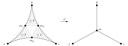
Let $(X,d)$ be a geodesic metric space. A geodesic triangle $\Delta(x,y,z)$ with $x,y,z\in X$ is the union $[x,y]\cup[x,z]\cup[y,z]$ of three geodesic segments connecting these vertices. Let $m_{x}$ be the point of the geodesic segment $[y,z]$ located at distance $\alpha_{y}:=(x|z)_{y}=(d(y,x)+d(y,z)-d(x,z))/2$ from $y.$ Then $m_{x}$ is located at distance $\alpha_{z}:=(y|x)_{z}=(d(z,y)+d(z,x)-d(y,x))/2$ from $z$ because $\alpha_{y}+\alpha_{z}=d(y,z)$. Analogously, define the points $m_{y}\in[x,z]$ and $m_{z}\in[x,y]$ both located at distance $\alpha_{x}:=(y|z)_{x}=(d(x,y)+d(x,z)-d(y,z))/2$ from $x;$ see Fig. 1 for an illustration. There exists a unique isometry $\varphi$ which maps $\Delta(x,y,z)$ to a tripod $T(x,y,z)$ consisting of three solid segments $[x,m],[y,m],$ and $[z,m]$ of lengths $\alpha_{x},\alpha_{y},$ and $\alpha_{z},$ respectively. This isometry maps the vertices $x,y,z$ of $\Delta(x,y,z)$ to the respective leaves of $T(x,y,z)$ and the points $m_{x},m_{y},$ and $m_{z}$ to the center $m$ of this tripod. Any other point of $T(x,y,z)$ is the image of exactly two points of $\Delta(x,y,z).$ A geodesic triangle $\Delta(x,y,z)$ is called $\delta$-thin if for all points $u,v\in\Delta(x,y,z),$ $\varphi(u)=\varphi(v)$ implies $d(u,v)\leq\delta.$ A graph $G=(V,E)$ whose all geodesic triangles $\Delta(u,v,w)$, $u,v,w\in V$, are $\delta$-thin is called a graph with $\delta$-thin triangles, and $\delta$ is called the thinness parameter of $G$.

Figure 1: A geodesic triangle $\Delta(x,y,z),$ the points $m_{x},m_{y},m_{z},$ and the tripod $\Upsilon(x,y,z)$

The following result shows that hyperbolicity of a geodesic space or a graph is equivalent to having thin geodesic triangles.

Proposition 1 ([14, 28, 59, 60])

Geodesic triangles of geodesic $\delta$-hyperbolic spaces or graphs are $4\delta$-thin. Conversely, geodesic spaces or graphs with $\delta$-thin triangles are $\delta$-hyperbolic.

In what follows, we will need few more notions and notations. Let $G=(V,E)$ be a graph. By $[x,y]$ we denote a shortest path connecting vertices $x$ and $y$ in $G$; we call $[x,y]$ a geodesic between $x$ and $y$. A ball $B(s,r)$ of $G$ centered at vertex $s\in V$ and with radius $r$ is the set of all vertices with distance no more than $r$ from $s$ (i.e., $B(s,r):=\{v\in V:d_{G}(v,s)\leq r\}$). The $k$th-power of a graph $G=(V,E)$ is the graph $G^{k}=(V,E^{\prime})$ such that $xy\in E^{\prime}$ if and only if $0<d_{G}(x,y)\leq k$. Denote by $F(x):=\{y\in V:d_{G}(x,y)=ecc_{G}(x)\}$ the set of all vertices of $G$ that are most distant from $x$. Vertices $x$ and $y$ of $G$ are called mutually distant if $x\in F(y)$ and $y\in F(x)$, i.e., $ecc_{G}(x)=ecc_{G}(y)=d_{G}(x,y)$.

3 Fast approximation of eccentricities

In this section, we give linear and almost linear time algorithms for sharp estimation of the diameters, the radii, the centers and the eccentricities of all vertices in graphs with $\delta$-thin triangles. Before presenting those algorithms, we establish some conditional lower bounds on complexities of computing the diameters and the radii in those graphs.

3.1 Conditional lower bounds on complexities

Recent work has revealed convincing evidence that solving the diameter problem in subquadratic time might not be possible, even in very special classes of graphs. Roditty and Vassilevska W. [83] showed that an algorithm that can distinguish between diameter 2 and 3 in a sparse graph in subquadratic time refutes the following widely believed conjecture.

The Orthogonal Vectors Conjecture: There is no $\epsilon>0$ such that for all $c\geq 1$, there is an algorithm that given two lists of $n$ binary vectors $A,B\subseteq\{0,1\}^{d}$ where $d=c\log n$ can determine if there is an orthogonal pair $a\in A,b\in B$, in $O(n^{2-e})$ time.

Williams [95] showed that the Orthogonal Vectors (OV) Conjecture is implied by the well-known Strong Exponential Time Hypothesis (SETH) of Impagliazzo, Paturi, and Zane [64, 63]. Nowadays many papers base the hardness of problems on SETH and the OV conjecture (see, e.g., [8, 21, 91] and papers cited therein).

Since all geodesic triangles of a graph constructed in the reduction in [83] are 2-thin, we can rephrase the result from [83] as follows.

Statement 1

If for some $\epsilon>0$, there is an algorithm that can determine if a given graph with 2-thin triangles, $n$ vertices and $m=O(n)$ edges has diameter 2 or 3 in $O(n^{2-\epsilon})$ time, then the Orthogonal Vector Conjecture is false.

To prove a similar lower bound result for the radius problem, recently Abboud et al. [8] suggested to use the following natural and plausible variant of the OV conjecture.

The Hitting Set Conjecture: There is no $\epsilon>0$ such that for all $c\geq 1$, there is an algorithm that given two lists $A,B$ of $n$ subsets of a universe $U$ of size $c\log n$, can decide in $O(n^{2-e})$ time if there is a set in the first list that intersects every set in the second list, i.e. a hitting set.

Abboud et al. [8] showed that an algorithm that can distinguish between radius 2 and 3 in a sparse graph in subquadratic time refutes the Hitting Set Conjecture. Since all geodesic triangles of a graph constructed in the reduction in [8] are 2-thin, rephrasing that result from [8], we have.

Statement 2

If for some $\epsilon>0$, there is an algorithm that can determine if a given graph with 2-thin triangles, $n$ vertices, and $m=O(n)$ edges has radius 2 or 3 in $O(n^{2-\epsilon})$ time, then the Hitting Set Conjecture is false.

3.2 Fast additive approximations

In this subsection, we show that in a graph $G$ with $\delta$-thin triangles the eccentricities of all vertices can be computed in total linear time with an additive error depending on $\delta$. We establish that the eccentricity of a vertex is determined (up-to a small error) by how far the vertex is from the center $C(G)$ of $G$. Finally, we show how to construct a spanning tree $T$ of $G$ in which the eccentricity of any vertex is its eccentricity in $G$ up to an additive error depending only on $\delta$. For these purposes, we revisit and extend several results from our previous paper [35] concerning the linear time approximation of diameter, radius, and centers of $\delta$-hyperbolic graphs. For these particular cases, we provide simplified proofs, leading to better additive errors due to the use of thinness of triangles instead of the four point condition and to the computation in $O(\delta|E|)$ time of a pair of mutually distant vertices.

Define the eccentricity layers of a graph $G$ as follows: for $k=0,\dots,diam(G)-rad(G)$ set

$$C^{k}(G):=\{v\in V:ecc_{G}(v)=rad(G)+k\}.$$

With this notation, the center of a graph is $C(G)=C^{0}(G)$. In what follows, it will be convenient to define also the eccentricity of the middle point $m$ of any edge $xy$ of $G$; set $ecc_{G}(m)=\min\{ecc_{G}(x),ecc_{G}(y)\}+1/2$.

We start with a proposition showing that, in a graph $G$ with $\delta$-thin triangles, a middle vertex of any geodesic between two mutually distant vertices has the eccentricity close to $rad(G)$ and is not too far from the center $C(G)$ of $G$.

Proposition 2

Let $G$ be a graph with $\delta$-thin triangles, $u,v$ be a pair of mutually distant vertices of $G$.

1. If $c^{*}$ is the middle point of any $(u,v)$-geodesic, then $ecc_{G}(c^{*})\leq\frac{d_{G}(u,v)}{2}+\delta\leq rad(G)+\delta$.

2. If $c$ is a middle vertex of any $(u,v)$-geodesic, then $ecc_{G}(c)\leq\lceil{\frac{d_{G}(u,v)}{2}}\rceil+\delta\leq rad(G)+\delta$.

3. $d_{G}(u,v)\geq 2rad(G)-2\delta-1$. In particular, $diam(G)\geq 2rad(G)-2\delta-1.$

4. If $c$ is a middle vertex of any $(u,v)$-geodesic and $x\in C^{k}(G),$ then $k-\delta\leq d_{G}(x,c)\leq k+2\delta+1$. In particular, $C(G)\subseteq B(c,2\delta+1)$.

Proof

Let $x$ be an arbitrary vertex of $G$ and $\Delta(u,v,x):=[u,v]\cup[v,x]\cup[x,u]$ be a geodesic triangle, where $[v,x],[x,u]$ are arbitrary geodesics connecting $x$ with $v$ and $u$. Let $m_{x}$ be a point on $[u,v]$ which is at distance $(x|u)_{v}=\frac{1}{2}(d(x,v)+d(v,u)-d(x,u))$ from $v$ and hence at distance $(x|v)_{u}=\frac{1}{2}(d(x,u)+d(v,u)-d(x,v))$ from $u$. Since $u$ and $v$ are mutually distant, we can assume, without loss of generality, that $c^{*}$ is located on $[u,v]$ between $v$ and $m_{x}$, i.e., $d(v,c^{*})\leq d(v,m_{x})=(x|u)_{v}$, and hence $(x|v)_{u}\leq(x|u)_{v}$. Since $d_{G}(v,x)\leq d_{G}(v,u)$, we also get $(u|v)_{x}\leq(x|v)_{u}$.

(a) By the triangle inequality and since $d_{G}(u,v)\leq diam(G)\leq 2rad(G)$, we get

$$d_{G}(x,c^{*}) \leq e(u|v)_{x}+\delta+d_{G}(u,c^{*})-(x|v)_{u}$$

$$\leq d_{G}(u,c^{*})+\delta=\frac{d_{G}(u,v)}{2}+\delta\leq rad(G)+\delta.$$

(b) Since $c^{*}=c$ when $d_{G}(u,v)$ is even and $d_{G}(c^{*},c)=\frac{1}{2}$ when $d_{G}(u,v)$ is odd, we have $ecc_{G}(c)\leq ecc_{G}(c^{*})+\frac{1}{2}$. Additionally to the proof of (a), one needs only to consider the case when $d_{G}(u,v)$ is odd. We know that the middle point $c^{*}$ sees all vertices of $G$ within distance at most $\frac{d_{G}(u,v)}{2}+\delta$. Hence, both ends of the edge of $(u,v)$-geodesic, containing the point $c^{*}$ in the middle, have eccentricities at most

$$\frac{d_{G}(u,v)}{2}+\frac{1}{2}+\delta=\lceil{\frac{d_{G}(u,v)}{2}}\rceil+\delta\leq\lceil{\frac{2rad(G)-1}{2}}\rceil+\delta=rad(G)+\delta.$$

(c) Since a middle vertex $c$ of any $(u,v)$-geodesic sees all vertices of $G$ within distance at most $\lceil{\frac{d_{G}(u,v)}{2}}\rceil+\delta$, if $d_{G}(u,v)\leq 2rad(G)-2\delta-2$, then

$$ecc_{G}(c)\leq\lceil{\frac{d_{G}(u,v)}{2}}\rceil+\delta\leq\lceil{\frac{2rad(G)-2\delta-2}{2}}\rceil+\delta<rad(G),$$

which is impossible.

(d) In the proof of (a), instead of an arbitrary vertex $x$, consider any vertex $x$ from $C^{k}(G)$. By the triangle inequality and since $d_{G}(u,v)\geq 2rad(G)-2\delta-1$ and both $d_{G}(u,x),d_{G}(x,v)$ are at most $rad(G)+k$, we get

$$d_{G}(x,c^{*}) \leq (u|v)_{x}+\delta+(x|u)_{v}-d_{G}(v,c^{*})=d_{G}(v,x)-d_{G}(v,c^{*})+\delta$$

$$\leq rad(G)+k-\frac{d_{G}(u,v)}{2}+\delta\leq k+2\delta+\frac{1}{2}.$$

Consequently, $d_{G}(x,c)\leq d_{G}(x,c^{*})+\frac{1}{2}\leq k+2\delta+1.$ On the other hand, since $ecc_{G}(x)\leq ecc_{G}(c)+d_{G}(x,c)$ and $ecc_{G}(c)\leq rad(G)+\delta$, by statement (a), we get

$$d_{G}(x,c) \geq ecc_{G}(x)-ecc_{G}(c)=k+rad(G)-ecc_{G}(c)$$

$$\geq (k+rad(G))-(rad(G)+\delta)=k-\delta.$$

∎

As an easy consequence of Proposition 2(d), we get that the eccentricity $ecc_{G}(x)$ of any vertex $x$ is equal, up to an additive one-sided error of at most $4\delta+2$, to $d_{G}(x,C(G))$ plus $rad(G)$.

Corollary 1

For every vertex $x$ of a graph $G$ with $\delta$-thin triangles,

$$d_{G}(x,C(G))+rad(G)-4\delta-2\leq ecc_{G}(x)\leq d_{G}(x,C(G))+rad(G).$$

Proof

Consider an arbitrary vertex $x$ in $G$ and assume that $ecc_{G}(x)=rad(G)+k$. Let $c_{x}$ be a vertex from $C(G)$ closest to $x$. By Proposition 2(d), $d_{G}(c,c_{x})\leq 2\delta+1$ and $d_{G}(x,c)\leq k+2\delta+1=ecc_{G}(x)-rad(G)+2\delta+1$. Hence,

$$d_{G}(x,C(G))=d_{G}(x,c_{x})\leq d_{G}(x,c)+d_{G}(c,c_{x})\leq d_{G}(x,c)+2\delta+1$$

and

$$ecc_{G}(x)\geq d_{G}(x,c)+rad(G)-2\delta-1.$$

Combining both inequalities, we get

$$ecc_{G}(x)\geq d_{G}(x,C(G))+rad(G)-4\delta-2.$$

Note also that, by the triangle inequality, $ecc_{G}(x)\leq d_{G}(x,c_{x})+ecc_{G}(c_{x})=d_{G}(x,C(G))+rad(G)$ (that is, the right-hand inequality holds for all graphs). ∎

It is interesting to note that the equality $ecc_{G}(x)=d_{G}(x,C(G))+rad(G)$ holds for every vertex of a graph $G$ if and only if the eccentricity function $ecc_{G}(\cdot)$ on $G$ is unimodal (that is, every local minimum is a global minimum)[48]. A slightly weaker condition holds for all chordal graphs [51]: for every vertex $x$ of a chordal graph $G$, $ecc_{G}(x)\geq d_{G}(x,C(G))+rad(G)-1$.

Proposition 3

Let $G$ be a graph with $\delta$-thin triangles and $u,v$ be a pair of vertices of $G$ such that $v\in F(u)$.

1. If $w$ is a vertex of a $(u,v)$-geodesic at distance $rad(G)$ from $v$, then $ecc_{G}(w)\leq rad(G)+\delta$.

2. For every pair of vertices $x,y\in V$, $\max\{d_{G}(v,x),d_{G}(v,y)\}\geq d_{G}(x,y)-2\delta$.

3. $ecc_{G}(v)\geq diam(G)-2\delta\geq 2rad(G)-4\delta-1$.

4. If $t\in F(v),$ $c$ is a vertex of a $(v,t)$-geodesic at distance $\lceil\frac{d_{G}(v,t)}{2}\rceil$ from $t$ and $x\in C^{k}(G)$, then $ecc_{G}(c)\leq rad(G)+3\delta$ and $k-3\delta\leq d_{G}(x,c)\leq k+3\delta+1$. In particular, $C(G)\subseteq B(c,3\delta+1)$.

Proof

(a) Let $x$ be a vertex of $G$ with $d_{G}(w,x)=ecc_{G}(w)$. Let $\Delta(u,v,x):=[u,v]\cup[v,x]\cup[x,u]$ be a geodesic triangle, where $[v,x],[x,u]$ are arbitrary geodesics connecting $x$ with $v$ and $u$. Let $m_{x}$ be a point on $[u,v]$ which is at distance $(x|u)_{v}=\frac{1}{2}(d(x,v)+d(v,u)-d(x,u))$ from $v$ and hence at distance $(x|v)_{u}=\frac{1}{2}(d(x,u)+d(v,u)-d(x,v))$ from $u$. We distinguish between two cases: $w$ is between $u$ and $m_{x}$ or $w$ is between $v$ and $m_{x}$ in $[u,v]$.

In the first case, by the triangle inequality and $d_{G}(u,x)\leq d_{G}(u,v)$ (and hence, $(u|x)_{v}\geq(u|v)_{x}$), we get

$$d_{G}(w,x)\leq rad(G)-(u|x)_{v}+\delta+(u|v)_{x}\leq rad(G)+\delta.$$

In the second case, by the triangle inequality and since $d_{G}(v,x)\leq diam(G)\leq 2rad(G)$, we get

$$d_{G}(w,x) \leq (u|x)_{v}-rad(G)+\delta+(u|v)_{x}$$

$$\leq d_{G}(x,v)-rad(G)+\delta$$

$$\leq 2rad(G)-rad(G)+\delta=rad(G)+\delta.$$

(b) Consider an arbitrary $(u,v)$-geodesic $[u,v]$. Let $\Delta(u,v,x):=[u,v]\cup[v,x]\cup[x,u]$ be a geodesic triangle, where $[v,x],[x,u]$ are arbitrary geodesics connecting $x$ with $v$ and $u$. Let $\Delta(u,v,y):=[u,v]\cup[v,y]\cup[y,u]$ be a geodesic triangle, where $[v,y],[y,u]$ are arbitrary geodesics connecting $y$ with $v$ and $u$.

Let $m_{x}$ be a point on $[u,v]$ which is at distance $(x|u)_{v}=\frac{1}{2}(d(x,v)+d(v,u)-d(x,u))$ from $v$ and hence at distance $(x|v)_{u}=\frac{1}{2}(d(x,u)+d(v,u)-d(x,v))$ from $u$. Let $m_{y}$ be a point on $[u,v]$ which is at distance $(y|u)_{v}=\frac{1}{2}(d(y,v)+d(v,u)-d(y,u))$ from $v$ and hence at distance $(y|v)_{u}=\frac{1}{2}(d(y,u)+d(v,u)-d(y,v))$ from $u$. Without loss of generality, assume that $m_{x}$ is on $[u,v]$ between $v$ and $m_{y}$.

Since $d_{G}(u,v)\geq d_{G}(u,x)$ (as $v\in F(u)$), we have $(u|v)_{x}\leq(u|x)_{v}$. By the triangle inequality, we get

$$d_{G}(x,y) \leq (u|v)_{x}+\delta+((y|u)_{v}-(u|x)_{v})+\delta+(u|v)_{y}$$

$$\leq (u|x)_{v}-(u|x)_{v}+2\delta+(y|u)_{v}+(u|v)_{y}$$

$$= d_{G}(v,y)+2\delta.$$

Consequently, $\max\{d_{G}(v,x),d_{G}(v,y)\}\geq d_{G}(v,y)\geq d_{G}(x,y)-2\delta.$

(c) Now, if $x,y$ is a diametral pair, i.e., $d_{G}(x,y)=diam(G)$, then, by (b) and Proposition 2(c),

$$ecc_{G}(v) \geq \max\{d_{G}(v,x),d_{G}(v,y)\}$$

$$\geq d_{G}(x,y)-2\delta=diam(G)-2\delta$$

$$\geq 2rad(G)-4\delta-1.$$

(d) Consider any $(v,t)$-geodesic $[v,t]$ and let $c^{*}$ be the middle point of it, $w$ be a vertex of $[v,t]$ at distance $rad(G)$ from $t$, and $c$ be a vertex of $[v,t]$ at distance $\lceil\frac{d_{G}(v,t)}{2}\rceil$ from $t$. We know by (a) that $ecc_{G}(w)\leq rad(G)+\delta$. Furthermore, since $2rad(G)\geq d_{G}(v,t)\geq 2rad(G)-4\delta-1$ (by (c)), $rad(G)\geq d_{G}(t,c)=\lceil\frac{d_{G}(v,t)}{2}\rceil\geq rad(G)-2\delta$. Hence,

$$d_{G}(w,c)=d_{G}(w,t)-d_{G}(c,t)\leq rad(G)-rad(G)+2\delta=2\delta,$$

implying

$$ecc_{G}(c)\leq d_{G}(w,c)+ecc_{G}(w)\leq rad(G)+3\delta.$$

Let now $x$ be an arbitrary vertex from $C^{k}(G)$, i.e., $ecc_{G}(x)\leq rad(G)+k$, for some integer $k\geq 0$. Consider a geodesic triangle $\Delta(t,v,x):=[t,v]\cup[v,x]\cup[x,t]$, where $[v,x],[x,t]$ are arbitrary geodesics connecting $x$ with $v$ and $t$. Let $m_{x}$ be a point on $[t,v]$ which is at distance $(x|t)_{v}=\frac{1}{2}(d(x,v)+d(v,t)-d(x,t))$ from $v$ and hence at distance $(x|v)_{t}=\frac{1}{2}(d(x,t)+d(v,t)-d(x,v))$ from $t$. Since, in what follows, we will use only the fact that $d_{G}(v,t)\geq 2rad(G)-4\delta-1$, we can assume, without loss of generality, that $c^{*}$ is located on $[t,v]$ between $v$ and $m_{x}$, i.e., $d(v,c^{*})\leq d(v,m_{x})=(x|t)_{v}$.

By the triangle inequality and since $d_{G}(v,t)\geq 2rad(G)-4\delta-1$ and both $d_{G}(t,x)$ and $d_{G}(x,v)$ are at most $rad(G)+k$, we get

$$d_{G}(x,c^{*}) \leq (t|v)_{x}+\delta+(x|t)_{v}-d_{G}(v,c^{*})=d_{G}(v,x)-d_{G}(v,c^{*})+\delta$$

$$\leq rad(G)+k-\frac{d_{G}(v,t)}{2}+\delta\leq k+3\delta+\frac{1}{2}.$$

Hence, $d_{G}(x,c)\leq d_{G}(x,c^{*})+\frac{1}{2}\leq k+3\delta+1.$ On the other hand, since $ecc_{G}(x)\leq ecc_{G}(c)+d_{G}(x,c)$ and $ecc_{G}(c)\leq rad(G)+3\delta$, we get

$$d_{G}(x,c) \geq ecc_{G}(x)-ecc_{G}(c)=k+rad(G)-ecc_{G}(c)$$

$$\geq (k+rad(G))-(rad(G)+3\delta)=k-3\delta.$$

∎

Proposition 4

For every graph $G$ with $\delta$-thin triangles, $diam(C^{k}(G))\leq 2k+2\delta+1.$ In particular, $diam(C(G))\leq 2\delta+1.$

Proof

Let $x,y$ be two vertices of $C^{k}(G)$ such that $d_{G}(x,y)=diam(C^{k}(G))$. Pick any $(x,y)$-geodesic and consider the middle point $m$ of it. Let $z$ be a vertex of $G$ such that $d_{G}(m,z)=ecc_{G}(m)$. Consider a geodesic triangle $\Delta(x,y,z):=[x,y]\cup[y,z]\cup[z,x]$, where $[z,x],[y,z]$ are arbitrary geodesics connecting $z$ with $x$ and $y$. Let $m_{z}$ be a point on $[x,y]$ which is at distance $(x|z)_{y}=\frac{1}{2}(d(x,y)+d(z,y)-d(x,z))$ from $y$ and hence at distance $(y|z)_{x}=\frac{1}{2}(d(x,y)+d(z,x)-d(y,z))$ from $x$. Without loss of generality, we can assume that $m$ is located on $[x,y]$ between $y$ and $m_{z}$.

Since $ecc_{G}(y)\leq rad(G)+k$, we have

$$d_{G}(m,z)=ecc_{G}(m)\geq rad(G)-\frac{1}{2}\geq ecc_{G}(y)-k-\frac{1}{2}\geq d_{G}(y,z)-k-\frac{1}{2}.$$

On the other hand, by the triangle inequality, we get

$$d_{G}(m,z) \leq (x|z)_{y}-d_{G}(y,m)+\delta+(x|y)_{z}=d_{G}(y,z)-d_{G}(y,m)+\delta$$

$$\leq d_{G}(y,z)-\frac{d_{G}(x,y)}{2}+\delta.$$

Hence, $d_{G}(x,y)\leq 2k+2\delta+1.$ ∎

3.2.1 Diameter and radius.

For an arbitrary connected graph $G=(V,E)$ and a given vertex $u\in V$, a most distant from $u$ vertex $v\in F(u)$ can be found in linear ($O(|E|)$) time by a breadth-first-search $BFS(u)$ started at $u$. A pair of mutually distant vertices of a connected graph $G=(V,E)$ with $\delta$-thin triangles can be computed in $O(\delta|E|)$ total time as follows. By Proposition 3(c), if $v$ is a most distant vertex from an arbitrary vertex $u$ and $t$ is a most distant vertex from $v$, then $d(v,t)\geq\mathop{\rm diam}(G)-2\delta$. Hence, using at most $O(\delta)$ breadth-first-searches, one can generate a sequence of vertices $v:=v_{1},t:=v_{2},v_{3},\dots v_{k}$ with $k\leq 2\delta+2$ such that each $v_{i}$ is most distant from $v_{i-1}$ (with, $v_{0}=u$) and $v_{k}$, $v_{k-1}$ are mutually distant vertices (the initial value $d(v,t)\geq\mathop{\rm diam}(G)-2\delta$ can be improved at most $2\delta$ times).

Thus, by Proposition 2 and Proposition 3, we get the following additive approximations for the radius and the diameter of a graph with $\delta$-thin triangles.

Corollary 2

Let $G=(V,E)$ be a graph with $\delta$-thin triangles.

1. There is a linear $(O(|E|))$ time algorithm which finds in $G$ a vertex $c$ with eccentricity at most $rad(G)+3\delta$ and a vertex $v$ with eccentricity at least $diam(G)-2\delta$. Furthermore, $C(G)\subseteq B(c,3\delta+1)$ holds.

2. There is an almost linear $(O(\delta|E|))$ time algorithm which finds in $G$ a vertex $c$ with eccentricity at most $rad(G)+\delta$. Furthermore, $C(G)\subseteq B(c,2\delta+1)$ holds.

3.2.2 All eccentricities.

In what follows, we will show that all vertex eccentricities of a graph with $\delta$-thin triangles can be also additively approximated in (almost) linear time.

Proposition 5

Let $G$ be a graph with $\delta$-thin triangles.

1. If $c$ is a middle vertex of any $(u,v)$-geodesic between a pair $u,v$ of mutually distant vertices of $G$ and $T$ is a $BFS(c)$-tree of $G$, then, for every vertex $x$ of $G$, $ecc_{G}(x)\leq ecc_{T}(x)\leq ecc_{G}(x)+3\delta+1.$

2. If $v$ is a most distant vertex from an arbitrary vertex $u$, $t$ is a most distant vertex from $v$, $c$ is a vertex of a $(v,t)$-geodesic at distance $\lceil\frac{d_{G}(v,t)}{2}\rceil$ from $t$ and $T$ is a $BFS(c)$-tree of $G$, then $ecc_{G}(x)\leq ecc_{T}(x)\leq ecc_{G}(x)+6\delta+1.$

Proof

(a) Let $x$ be an arbitrary vertex of $G$ and assume that $ecc_{G}(x)=rad(G)+k$ for some integer $k\geq 0$. We know from Proposition 2(b) that $ecc_{G}(c)\leq rad(G)+\delta$. Furthermore, by Proposition 2(d), $d_{G}(c,x)\leq k+2\delta+1$. Since $T$ is a $BFS(c)$-tree, $d_{G}(x,c)=d_{T}(x,c)$ and $ecc_{G}(c)=ecc_{T}(c)$. Consider a vertex $y$ in $G$ such that $d_{T}(x,y)=ecc_{T}(x).$ We have

$$ecc_{T}(x) = d_{T}(x,y)\leq d_{T}(x,c)+d_{T}(c,y)$$

$$\leq d_{G}(x,c)+ecc_{T}(c)=d_{G}(x,c)+ecc_{G}(c)$$

$$\leq k+2\delta+1+rad(G)+\delta=rad(G)+k+3\delta+1$$

$$= ecc_{G}(x)+3\delta+1.$$

As $T$ is a spanning tree of $G$, evidently, also $ecc_{G}(x)\leq ecc_{T}(x)$ holds.

(b) The proof is similar to the proof of (a); only, in this case, $ecc_{G}(c)\leq rad(G)+3\delta$ and $d_{G}(c,x)\leq k+3\delta+1$ holds for every $x\in C^{k}(G)$ (by Proposition 3(d)). ∎

A spanning tree $T$ of a graph $G$ is called an eccentricity $k$-approximating spanning tree if for every vertex $v$ of $G$ $ecc_{T}(v)\leq ecc_{G}(v)+k$ holds [51, 81]. Thus, by Proposition 5, we get.

Theorem 3.1

Every graph $G=(V,E)$ with $\delta$-thin triangles admits an eccentricity $(3\delta+1)$-approximating spanning tree constructible in $O(\delta|E|)$ time and an eccentricity $(6\delta+1)$-approximating spanning tree constructible in $O(|E|)$ time.

Theorem 3.1 generalizes recent results from [51, 81] that chordal graphs and some of their generalizations admit eccentricity 2-approximating spanning trees.

Note that the eccentricities of all vertices in any tree $T=(V,U)$ can be computed in $O(|V|)$ total time. As we noticed already, it is a folklore by now that for trees the following facts are true:

• The center $C(T)$ of any tree $T$ consists of one vertex or two adjacent vertices.

• The center $C(T)$ and the radius $rad(T)$ of any tree $T$ can be found in linear time.

• For every vertex $v\in V$, $ecc_{T}(v)=d_{T}(v,C(T))+rad(T)$.

Hence, using $BFS(C(T))$ on $T$ one can compute $d_{T}(v,C(T))$ for all $v\in V$ in total $O(|V|)$ time. Adding now $rad(T)$ to $d_{T}(v,C(T))$, one gets $ecc_{T}(v)$ for all $v\in V$. Consequently, by Theorem 3.1, we get the following additive approximations for the vertex eccentricities in graphs with $\delta$-thin triangles.

Theorem 3.2

Let $G=(V,E)$ be a graph with $\delta$-thin triangles.

1. There is an algorithm which in total linear $(O(|E|))$ time outputs for every vertex $v\in V$ an estimate $\hat{e}(v)$ of its eccentricity $ecc_{G}(v)$ such that $ecc_{G}(v)\leq\hat{e}(v)\leq ecc_{G}(v)+6\delta+1.$

2. There is an algorithm which in total almost linear $(O(\delta|E|))$ time outputs for every vertex $v\in V$ an estimate $\hat{e}(v)$ of its eccentricity $ecc_{G}(v)$ such that $ecc_{G}(v)\leq\hat{e}(v)\leq ecc_{G}(v)+3\delta+1.$

4 Fast Additive Approximation of All Distances

Here, we will show that if the $\delta$th power $G^{\delta}$ of a graph $G$ with $\delta$-thin triangles is known in advance, then the distances in $G$ can be additively approximated (with an additive one-sided error of at most $\delta+1$) in $O(|V|^{2})$ time. If $G^{\delta}$ is not known, then the distances can be additively approximated (with an additive one-sided error of at most $2\delta+2$) in almost quadratic time.

Our method is a generalization of an unified approach used in [49] to estimate (or compute exactly) all pairs shortest paths in such special graph families as $k$-chordal graphs, chordal graphs, AT-free graphs and many others. For example: all distances in $k$-chordal graphs with an additive one-sided error of at most $k-1$ can be found in $O(|V|^{2})$ time; all distances in chordal graphs with an additive one-sided error of at most 1 can be found in $O(|V|^{2})$ time and the all pairs shortest path problem on a chordal graph $G$ can be solved in $O(|V|^{2})$ time if $G^{2}$ is known. Note that in chordal graph all geodesic triangles are 2-thin.

Let $G=(V,E)$ be a graph with $\delta$-thin triangles. Pick an arbitrary start vertex $s\in V$ and construct a $BFS(s)$-tree $T$ of $G$ rooted at $s$. Denote by $p_{T}(x)$ the parent and by $h_{T}(x)=d_{T}(x,s)=d_{G}(x,s)$ the height of a vertex $x$ in $T$. Since we will deal only with one tree $T$, we will often omit the subscript $T$. Let $P_{T}(x,s):=(x_{q},x_{q-1},\dots,x_{1},s)$ and $P_{T}(y,s):=(y_{p},y_{p-1},\dots,y_{1},s)$ be the paths of $T$ connecting vertices $x$ and $y$ with the root $s$. By $sl_{T}(x,y;\lambda)$ we denote the largest index $k$ such that $d_{G}(x_{k},y_{k})\leq\lambda$ (the $\lambda$ separation level). Our method is based on the following simple fact.

Proposition 6

For every vertices $x$ and $y$ of a graph $G$ with $\delta$-thin triangles and any $BFS$-tree $T$ of $G$,

$$h_{T}(x)+h_{T}(y)-2k-1\leq d_{G}(x,y)\leq h_{T}(x)+h_{T}(y)-2k+d_{G}(x_{k},y_{k}),$$

where $k=sl_{T}(x,y;\delta)$.

Proof

By the triangle inequality, $d_{G}(x,y)\leq d_{G}(x,x_{k})+d_{G}(x_{k},y_{k})+d_{G}(y_{k},y)=h_{T}(x)+h_{T}(y)-2k+d_{G}(x_{k},y_{k})$. Consider now an arbitrary $(x,y)$-geodesic $[x,y]$ in $G$. Let $\Delta(x,y,s):=[x,y]\cup[x,s]\cup[y,s]$ be a geodesic triangle, where $[x,s]=P_{T}(x,s)$ and $[y,s]=P_{T}(y,s)$. Since $\Delta(x,y,s)$ is $\delta$-thin, $sl_{T}(x,y;\delta)\geq(x|y)_{s}-\frac{1}{2}$. Hence, $h_{T}(x)-sl_{T}(x,y;\delta)\leq(s|y)_{x}+\frac{1}{2}$ and $h_{T}(y)-sl_{T}(x,y;\delta)\leq(s|x)_{y}+\frac{1}{2}$. As $d_{G}(x,y)=(s|y)_{x}+(s|x)_{y}$, we get $d_{G}(x,y)\geq h_{T}(x)-sl_{T}(x,y;\delta)+h_{T}(y)-sl_{T}(x,y;\delta)-1$. ∎

Note that we may regard $BFS(s)$ as having produced a numbering from $n$ to 1 in decreasing order of the vertices in $V$ where vertex $s$ is numbered $n$. As a vertex is placed in the queue by $BFS(s)$, it is given the next available number. The last vertex visited is given the number 1. Let $\sigma:=[v_{1},v_{2},\dots,v_{n}=s]$ be a $BFS(s)$-ordering of the vertices of $G$ and $T$ be a $BFS(s)$-tree of $G$ produced by a $BFS(s)$. Let $\sigma(x)$ be the number assigned to a vertex $x$ in this $BFS(s)$-ordering. For two vertices $x$ and $y$, we write $x<y$ whenever $\sigma(x)<\sigma(y)$.

First, we will show that if $G^{\delta}$ is known in advance (i.e., its adjacency matrix is given) for a graph $G$ with $\delta$-thin triangles, then the distances in $G$ can be additively approximated (with an additive one-sided error of at most $\delta+1$) in $O(|V|^{2})$ time. We consider the vertices of $G$ in the order $\sigma$ from 1 to $n$. For each current vertex $x$ we show that the values $\widehat{d}(x,y):=h_{T}(x)+h_{T}(y)-2sl_{T}(x,y;\delta)+\delta$ for all vertices $y$ with $y>x$ can be computed in $O(|V|)$ total time. By Proposition 6,

$$d_{G}(x,y)\leq\widehat{d}(x,y)\leq d_{G}(x,y)+\delta+1.$$

The values $\widehat{d}(x,y)$ for all $y$ with $y>x$ can be computed using the following simple procedure. We will omit the subscripts $G$ and $T$ if no ambiguities arise. Let also $L_{i}=\{v\in V:d(v,s)=i\}$. In the procedure, $S_{u}$ represents vertices of a subtree of $T$ rooted at $u$.

(01)          set $q:=h(x)$
(02)          define a set $S_{u}:=\{u\}$ for each vertex $u\in L_{q}$, $u>x$, and denote this family of sets by $\cal F$
(03)          for $k=q$ downto 0
(04)              let $x_{k}$ be the vertex from $L_{k}\cap P_{T}(x,s)$
(05)              for each vertex $u\in L_{k}$ with $u>x$
(06)                  if $d_{G}(u,x_{k})\leq\delta$ (i.e., $u=x_{k}$ or $u$ is adjacent to $x_{k}$ in $G^{\delta}$) then
(07)                       for every $v\in S_{u}$
(08)                           set $\widehat{d}(x,v):=h(x)+h(v)-2k+\delta$ and remove $S_{u}$ from $\cal F$
(09)                       endfor
(10)              endfor
(11)              /* update $\cal F$ for the next iteration */
(12)              if $k>0$ then
(13)                  for each vertex $u\in L_{k-1}$
(14)                       combine all sets $S_{u_{1}},\dots,S_{u_{\ell}}$ from $\cal F$ ($\ell\geq 0$), such that $p_{T}(u_{1})=\ldots=p_{T}(u_{\ell})=u$,
(15)                       into one new set $S_{u}:=\{u\}\cup S_{u_{1}}\cup\ldots\cup S_{u_{\ell}}$        /* when $\ell=0$, $S_{u}:=\{u\}$ */ (16)                  endfor
(17)          endfor
(18)          set also $\widehat{d}(x,s):=h(x)$.

Thus, we have the following result.

Theorem 4.1

Let $G=(V,E)$ be a graph with $\delta$-thin triangles. Given $G^{\delta}$, all distances in $G$ with an additive one-sided error of at most $\delta+1$ can be found in $O(|V|^{2})$ time.

To avoid the requirement that $G^{\delta}$ is given in advance, we can use any known fast constant-factor approximation algorithm that in total $T(|V|)$-time computes for every pair of vertices $x,y$ of $G$ a value $\widetilde{d}(x,y)$ such that $d_{G}(x,y)\leq\widetilde{d}(x,y)\leq\alpha d_{G}(x,y)+\beta$. We can show that, using such an algorithm as a preprocessing step, the distances in a graph $G$ with $\delta$-thin triangles can be additively approximated with an additive one-sided error of at most $\alpha\delta+\beta+1$ in $O(T(|V|)+|V|^{2})$ time.

Although one can use any known fast constant-factor approximation algorithm in the preprocessing step, in what follows, we will demonstrate our idea using a fast approximation algorithm from [19]. It computes in $O(|V|^{2}\log^{2}|V|)$ total time for every pair $x,y$ a value $\widetilde{d}(x,y)$ such that

$$d_{G}(x,y)\leq\widetilde{d}(x,y)\leq 2d_{G}(x,y)+1.$$

Assume that the values $\widetilde{d}(x,y)$, $x,y\in V$, are precomputed. By $\widetilde{sl}_{T}(x,y;\lambda)$ we denote now the largest index $k$ such that $\widetilde{d}_{G}(x_{k},y_{k})\leq\lambda$. We have

Proposition 7

For every vertices $x$ and $y$ of a graph $G$ with $\delta$-thin triangles, any integer $\rho\geq\delta$, and any $BFS$-tree $T$ of $G$,

$$h_{T}(x)+h_{T}(y)-2k-1\leq d_{G}(x,y)\leq h_{T}(x)+h_{T}(y)-2k+d_{G}(x_{k},y_{k}),$$

where $k=\widetilde{sl}_{T}(x,y;2\rho+1)$.

Proof

The proof is identical to the proof of Proposition 7. One needs only to notice the following. In a geodesic triangle $\Delta(x,y,s):=[x,y]\cup[x,s]\cup[y,s]$ with $[x,s]=P_{T}(x,s)=(x_{q},x_{q-1},\dots,x_{1},s)$ and $[y,s]=P_{T}(y,s)=(y_{p},y_{p-1},\dots,y_{1},s)$, for each $i\leq(x|y)_{s}$, $d_{G}(x_{i},y_{i})\leq\delta\leq\rho$ and, hence, $\widetilde{d}(x_{i},y_{i})\leq 2\rho+1$ holds. Therefore, $\widetilde{sl}_{T}(x,y;2\rho+1)\geq(x|y)_{s}-\frac{1}{2}$. ∎

Let $\rho$ be any integer greater than or equal to $\delta$. By replacing in our earlier procedure lines (06) and (08) with

(06)^′          if $\widetilde{d}(u,x_{k})\leq 2\rho+1$ then
(08)^′          set $\widehat{d}(x,v):=h(x)+h(v)-2k+2\rho+1$ and remove $S_{u}$ from $\cal F$

we will compute for each current vertex $x$ all values $\widehat{d}(x,y):=h_{T}(x)+h_{T}(y)-2\widetilde{sl}_{T}(x,y;2\rho+1)+2\rho+1$, $y>x$, in $O(|V|)$ total time. By Proposition 7,

$$d_{G}(x,y) \leq h_{T}(x)+h_{T}(y)-2\widetilde{sl}_{T}(x,y;2\rho+1)+d_{G}(x_{k},y_{k})$$

$$\leq h_{T}(x)+h_{T}(y)-2\widetilde{sl}_{T}(x,y;2\rho+1)+\widetilde{d}(x_{k},y_{k})$$

$$\leq h_{T}(x)+h_{T}(y)-2\widetilde{sl}_{T}(x,y;2\rho+1)+2\rho+1$$

$$= \widehat{d}(x,y)$$

and

$$\widehat{d}(x,y) = h_{T}(x)+h_{T}(y)-2\widetilde{sl}_{T}(x,y;2\rho+1)+2\rho+1$$

$$\leq d_{G}(x,y)+2\rho+2.$$

Thus, we have the following result:

Theorem 4.2

Let $G=(V,E)$ be a graph with $\delta$-thin triangles.

1. If the value of $\delta$ is known, then all distances in $G$ with an additive one-sided error of at most $2\delta+2$ can be found in $O(|V|^{2}\log^{2}|V|)$ time.

2. If an approximation $\rho$ of $\delta$ such that $\delta\leq\rho\leq a\delta+b$ is known (where $a$ and $b$ are constants), then all distances in $G$ with an additive one-sided error of at most $2(a\delta+b+1)$ can be found in $O(|V|^{2}\log^{2}|V|)$ time.

The second part of Theorem 4.2 says that if an approximation of the thinness parameter of a graph $G$ is given then all distances in $G$ can be additively approximated in $O(|V|^{2}\log^{2}|V|)$ time. Recently, it was shown in [32] that the following converse is true. From an estimate of all distances in $G$ with an additive one-sided error of at most $k$, it is possible to compute in $O(|V|^{2})$ time an estimation $\rho^{*}$ of the thinness of $G$ such that $\delta\leq\rho^{*}\leq 8\delta+12k+4,$ proving a $\tilde{O}(|V|^{2})$-equivalence between approximating the thinness and approximating the distances in graphs.

5 Experimentation on Some Real-World Networks

In this section, we analyze the performance of our algorithms for approximating eccentricities and distances on a number of real-world networks. Our experimental results show that the estimates on eccentricities and distances obtained are even better than the theoretical bounds described in Corollary 2 and Theorems 3.2,4.2.

Network	Type	Ref.	$|V|$	$|E|$	$|C(G)|$	$\overline{deg}$	$rad(G)$	$diam(G)$	$diam_{G}(C(G))$	connected?	$\delta(G)$
dutch-elite	social	[17]	3621	4310	3	2.4	12	22	4	no	5
facebook		[74]	4039	88234	1	43.7	4	8	0	yes	1.5
eva		[17]	4475	4664	15	2.1	10	18	3	yes	3.5
slashdot		[73]	77360	905468	1	13.1	6	12	0	yes	*1.5
loans		[71]	89171	3394979	29350	74.69	5	8	4	yes
twitter		[45]	465017	834797	755	3.59	5	8	4	yes
email-virgili		[61]	1133	5451	215	9.6	5	8	4	yes	2
email-enron	communi-	[73, 68]	33696	180811	248	10.7	7	13	2	yes
email-eu	cation	[72]	224832	680720	1	$\approx 3$	7	14	0	yes
wikitalk-china		[87]	1217365	3391055	17	2.9	4	8	2	yes
cs-metabolic	biological	[55]	453	4596	17	8.9	4	7	2	yes	1.5
sc-ppi		[65]	1458	1948	48	2.7	11	19	6	no	3.5
yeast-ppi		[29]	2224	6609	57	$\approx 6$	6	11	4	no	2.5
homo-pi		[86]	16635	115364	135	13.87	5	10	2	no	2
as-graph-1	internet	[3]	3015	5156	32	3.4	5	9	2	yes	2
as-graph-2		[3]	4885	9276	531	3.8	6	11	4	no	3
as-graph-3		[3]	5357	10328	10	3.9	5	9	2	yes	2
routeview		[7]	10515	21455	2	4.1	5	10	2	no	2.5
as-caida		[5]	26475	53381	2	4.03	9	17	1	yes	2.5
itdk		[4]	190914	607610	155	6.4	14	26	4	yes
gnutella-06	peer-to-peer	[82, 72]	8717	31525	338	7.2	6	10	5	no	3
gnutella-24		[82, 72]	26498	65359	1	4.9	6	11	0	yes	3
gnutella-30		[82, 72]	36646	88303	602	4.8	7	11	6	no	*2.5
gnutella-31		[82, 72]	62561	295756	55	4.7	7	11	5	no	*2.5
web-stanford	web	[73]	255265	2234572	1	15.2	82	164	0	yes	*7
web-notredam		[13]	325729	1497134	12	6.8	23	46	2	no	*2
web-berkstan		[73]	654782	7600595	1	20.1	104	208	0	yes	*7
amazon-1	product	[96]	334863	925872	21	5.5	24	47	3	no
amazon-2	co-purchasing	[96]	400727	3200440	194	11.7	11	20	5	no
road-euro	infrastructure	[88]	1039	1305	1	2.5	31	62	0	yes	7.5
openflight		[6]	3397	19231	21	11.3	7	13	2	yes	2
power-grid		[93]	4941	6594	1	2.7	23	46	0	yes	10
road-pa		[73]	1087562	3083028	2	2.83	402	794	1	yes	*195.5

Table 1: Statistics of the analyzed networks: $|V|$ is the number of vertices, $|E|$ is the number of edges; $|C(G)|$ is the number of central vertices; $\overline{deg}$ is the average degree; $rad(G)$ is the graph’s radius; $diam(G)$ is the graph’s diameter; $diam_{G}(C(G))$ is the diameter of the graph’s center; ”connected?” indicates whether or not the center of the graph is connected; $\delta(G)$ is the graph’s hyperbolicity. Hyperbolicity values marked with asterisks are approximate.

We apply our algorithms to six social networks, four email communication networks, four biological networks, six internet graphs, four peer-to-peer networks, three web networks, two product-co-purchasing networks, and four infrastructure networks. Most of the networks listed are part of the Stanford Large Network Dataset Collection (snap) and the Koblenz Network Collection (konect), and are available at [1] and [2]. Characteristics of these networks, such as the number of vertices and edges, the average degree, the radius and the diameter, are given in Table 1. The numbers listed in Table 1 are based on the largest connected component of each network, when the entire network is disconnected. We ignore the directions of the edges and remove all self-loops from each network. Additionally, in Table 1, for each network we report the size (as the number of vertices) of its center $C(G)$. We also analyze the diameter and the connectivity of the center of each network. The diameter of the center $diam_{G}(C(G))$ is defined as the maximum distance between any two central vertices in the graph. In the last column of Table 1, we report the Gromov hyperbolicity $\delta$ of majority of networks. Computing the hyperbolicity of a graph is computationally expensive; therefore, we provide the exact $\delta$ values for the smaller networks (those with $|V|\leq 30$K) in our dataset (in some cases, the algorithm proposed in [41] was used). For some larger networks, the approximated $\delta$-hyperbolicity values listed in Table 1 are as reported in [67]. Most networks that we included in our dataset are hyperbolic. However, for comparison reasons, we included also a few infrastructure networks that are known to lack the hyperbolicity property.

5.1 Estimation of Eccentricities

Following Proposition 2, for each graph in our dataset, we found a pair $u,v$ of mutually distant vertices. In column two of Table 2, we report on how many $BFS$ sweeps of a graph were needed to locate $u$ and $v$. Interestingly, for almost all graphs (28 out 33) only two sweeps were sufficient. For four other graphs (including road-pa network whose hyperbolicity is large) three sweeps were needed, and only for one graph (power-grid network) we needed four sweeps.

Network	No. of BFS iterations	$d_{G}(u,v)$	$2rad(G)-d_{G}(u,v)$	$ecc_{G}(c)$	$ecc_{G}(c)-rad(G)$	$d_{G}(c,C(G))$	$\min i:$ $B(c,i)\supseteq C(G)$	$k_{max}$	$k_{avg}$
		Prop.2(c)	Prop.2(c)	Prop.2(b)	Prop.2(b)	Prop.2(d)
dutch-elite	2	22	2	13	1	1	3	6	2.35
facebook	2	8	0	4	0	0	0	2	0.686
eva	2	18	2	10	0	0	2	2	0.571
slashdot	2	11	1	7	1	2	2	3	1.777
loans	2	7	3	5	0	0	3	3	2.06
twitter	2	8	2	6	1	1	3	4	2.569
email-virgili	2	7	3	6	1	1	3	4	2.729
email-enron	2	13	1	7	0	0	2	2	0.906
email-eu	2	14	0	7	0	0	0	2	0.002
wikitalk-china	2	7	1	5	1	1	2	3	2.076
ce-metabolic	2	7	1	5	1	1	2	3	1.982
sc-ppi	3	19	3	12	1	2	6	3	0.981
yeast-ppi	3	11	1	6	0	0	3	3	1.872
homo-pi	2	10	0	5	0	0	2	2	0.747
as-graph-1	2	8	2	6	1	1	2	3	1.791
as-graph-2	3	11	1	6	0	0	3	3	1.124
as-graph-3	2	9	1	5	0	0	2	2	0.828
routeview	2	10	0	5	0	0	2	2	0.329
as-caida	2	17	1	9	0	0	1	0	0
itdk	2	26	2	15	1	1	3	4	2.108
gnutella-06	2	10	2	6	0	0	4	4	2.507
gnutella-24	2	10	2	7	1	1	1	5	2.697
gnutella-30	2	11	3	7	0	0	5	5	3.167
gnutella-31	2	11	3	8	1	2	5	6	4.176
web-stanford	2	164	0	82	0	0	0	28	0.006
web-notredam	2	46	0	23	0	0	2	2	0.935
web-berkstan	2	208	0	104	0	0	0	22	0.002
amazon-1	2	47	1	24	0	0	2	6	0.991
amazon-2	2	20	2	12	1	2	5	6	3.735
road-euro	2	62	0	31	0	0	0	8	0.135
openflight	2	13	1	8	1	1	2	3	1.879
power-grid	4	46	0	28	5	8	8	13	5.735
road-pa	3	794	10	415	13	44	45	98	23.339

Table 2: Qualities of a pair of mutually distant vertices $u$ and $v$, of a middle vertex $c$ of a $(u,v)$-geodesic, and of a $BFS(c)$-tree $T_{1}$ rooted at vertex $c$. ”No. of BFS iterations“ indicates how many breadth-first-search iterations were needed to obtain a pair of mutually distant vertices $u$ and $v$. For each vertex $x\in V$, $k(x):=ecc_{T_{1}}(x)-ecc_{G}(x)$. Also, $k_{max}:=\max_{x\in V}k(x)$ and $k_{avg}:=\frac{1}{n}\sum_{x\in V}k(x)$.

In column four of Table 2, we report for each graph $G$ the difference between $2rad(G)$ and $d_{G}(u,v)$. Proposition 2(c) says that the difference must be at most $2\delta+1$, where $\delta$ is the thinness of geodesic triangles in $G$. Actually, for large number (27 out of 33) of graphs in our dataset, the difference is at most two. Five other graphs have the difference equal to 3, and only road-pa network has the difference equal to 10. We have $d_{G}(u,v)=diam(G)$ for 27 graphs in our dataset, including road-pa network whose geodesic triangles thinness is at least 196. For remaining six graphs $d_{G}(u,v)=diam(G)-1$ holds.

We also analyzed the quality of a middle vertex $c$ of a randomly picked shortest path between mutually distant vertices $u$ and $v$. Proposition 2 states that $ecc_{G}(c)$ is close to $rad(G)$ and $c$ is not too far from the graph’s center $C(G)$. Table 2 lists the properties of the selected middle vertex $c$. In almost all graphs, vertex $c$ belongs to the center $C(G)$ or is at distance one or two from $C(G)$. Even in graphs with $ecc_{G}(c)-rad(G)>2$ (power-grid and road-pa), the value $ecc_{G}(c)-rad(G)$ is smaller than what is suggested by Proposition 2(b). It is also clear from Table 2 that $c$ is not too far from any vertex in $C(G)$ (look at the radius $i$ of the ball $B(c,i)$ required to include $C(G)$). In all graphs, $i$ is much smaller than $2\delta+1$ (indicated in Proposition 2(d)).

Network	$ecc_{G}(v)$	$2rad(G)-ecc_{G}(v)$	$ecc_{G}(w)$	$d_{G}(w,C(G))$	$\min i:$ $B(w,i)\supseteq C(G)$	$k_{max}$	$k_{avg}$
		Prop.3(c)	Prop.3(a)
dutch-elite	22	2	12	0	4	6	2.431
facebook	8	0	5	3	3	3	0.704
eva	18	2	11	1	3	2	0.572
slashdot	11	1	7	2	2	3	1.88
loans	7	3	5	0	3	3	2.031
twitter	8	2	5	0	3	3	1.821
email-virgili	7	3	5	0	4	4	1.932
email-enron	13	1	7	0	2	2	0.903
email-eu	14	0	7	0	0	2	0.002
wikitalk-china	8	0	5	1	2	3	1.791
ce-metabolic	7	1	4	0	1	1	0.349
sc-ppi	19	3	12	1	6	7	4.196
yeast-ppi	11	1	7	1	3	4	2.558
homo-pi	9	1	5	0	2	2	0.612
as-graph-1	9	1	5	0	2	2	0.887
as-graph-2	11	1	6	0	3	2	0.833
as-graph-3	9	1	5	0	2	2	0.312
routeview	10	0	5	0	2	2	0.329
as-caida	17	1	9	0	1	0	0
itdk	26	2	15	1	3	5	2.702
gnutella-06	10	2	7	1	5	5	3.543
gnutella-24	11	1	8	3	3	6	4.475
gnutella-30	11	3	8	1	5	6	4.034
gnutella-31	11	3	8	1	5	6	4.251
web-stanford	164	0	82	0	0	28	0.006
web-notredam	46	0	23	0	2	2	0.935
web-berkstan	208	0	104	0	0	22	0.002
amazon-1	47	1	24	0	3	7	0.919
amazon-2	20	2	11	0	5	5	2.03
road-euro	62	0	31	0	0	8	0.135
openflight	13	1	7	0	2	2	0.641
power-grid	46	0	23	0	0	4	1.409
road-pa	772	32	417	21	22	80	22.545

Table 3: Qualities of a vertex $v$ most distant from a random vertex $u$, of a vertex $w$ of a $(u,v)$-geodesic at distance $rad(G)$ from $v$, and of a $BFS(w)$-tree $T_{2}$ rooted at vertex $w$. For each vertex $x\in V$, $k(x):=ecc_{T_{2}}(x)-ecc_{G}(x)$. Also, $k_{max}:=\max_{x\in V}k(x)$ and $k_{avg}:=\frac{1}{n}\sum_{x\in V}k(x)$.

Following Theorem 3.1, for each graph $G=(V,E)$ in our dataset, we constructed an arbitrary $BFS(c)$-tree $T_{1}=(V,E^{\prime})$, rooted at vertex $c$, and analyzed how well $T_{1}$ preserves or approximates the eccentricities of vertices in $G$. By Theorem 3.1, $ecc_{G}(v)\leq ecc_{T_{1}}(v)\leq ecc_{G}(v)+3\delta+1$ holds for every $v\in V$. In our experiments, for each graph $G$ and the constructed for it $BFS(c)$-tree $T_{1}$, we computed $k_{max}:=\max_{v\in V}\{ecc_{T_{1}}(v)-ecc_{G}(v)\}$ (maximum distortion) and $k_{avg}:=\frac{1}{n}\sum_{v\in V}ecc_{T_{1}}(v)-ecc_{G}(v)$ (average distortion). For most graphs (see Table 2), the value of $k_{max}$ is small: $k_{max}=0$ for one graph, $k_{max}=2$ for eight graphs, $k_{max}=3$ for nine graphs, $k_{max}=4$ for four graphs, $k_{max}=5$ for two graphs, and $k_{max}>5$ for nine graphs. Also, the average distortion $k_{avg}$ is much smaller than $k_{max}$ for all graphs. In fact, $k_{avg}<3$ in all but five graphs (gnutella-30, gnutella-31, amazon-2, power-grid, and road-pa). In graphs with high $k_{max}$, close inspection reveals that only small percent of vertices achieve this maximum. For example, in graph web-stanford, $k_{max}=28$ was only achieved by 17 vertices. The distributions of the values of $k(v):=ecc_{T_{1}}(v)-ecc_{G}(v)$ of all graphs are listed in Table 6 (see Appendix).

Similar experiments were performed following Proposition 3. For each graph $G$ in our dataset, we picked a random vertex $u\in V$ and a random vertex $v\in F(u)$. Then, we identified in a randomly picked $(u,v)$-geodesic a vertex $w$ at distance $rad(G)$ from $v$. We did not consider a vertex $c$ defined in Proposition 3(d) since, for majority of graphs in our dataset, $c$ will be a middle vertex of a geodesic between two mutually distant vertices, and working with $c$ we will duplicate previous experiments. Recall that for majority of our graphs (as found in our experiments) two BFS sweeps already identify a pair of mutually distant vertices. We know from Proposition 3 that $ecc_{G}(v)\geq diam(G)-2\delta\geq 2rad(G)-4\delta-1$ and $ecc_{G}(w)\leq rad(G)+\delta$. Our experimental results are better than these theoretical bounds. In Table 3, we list eccentricities of $v$ and $w$ for each graph. In almost all graphs, the eccentricity of $v$ is equal to the diameter $diam(G)$. Only four graphs have $ecc_{G}(v)=diam(G)-1$ and one graph (road-pa) has $ecc_{G}(v)>diam(G)-1$. Vertex $w$ is central for 21 graphs, has eccentricity equal to $rad(G)+1$ for 10 graphs, has eccentricity equal to $rad(G)+2$ for one graph, and only for one remaining graph (road-pa network, which has large hyperbolicity) its eccentricity is equal to $rad(G)+15$. It turns out also (see columns five and six of Table 2) that vertex $w$ either belongs to the center $C(G)$ or is very close to the center. The only exception is again road-pa network where $2rad(G)-ecc_{G}(w)=32$ and $d(w,C(G))=21$.

For every graph $G=(V,E)$ in our dataset, we constructed also an arbitrary $BFS(w)$-tree $T_{2}=(V,E^{\prime})$, rooted at vertex $w$, and analyzed how well $T_{2}$ preserves or approximates the eccentricities of vertices in $G$. The value of $k_{max}$ is at most five for 23 graphs. The average distortion $k_{avg}$ is much smaller than $k_{max}$ in all graphs. The distributions of the values of $k(x)$ for all graphs are presented in Table 7 (see Appendix).

Network	$diam(G)$	$diam(T_{1})$	$k_{max}^{T_{1}}$	$k_{avg}^{T_{1}}$	$diam(T_{2})$	$k_{max}^{T_{2}}$	$k_{avg}^{T_{2}}$	$diam(T_{3})$	$k_{max}^{T_{3}}$	$k_{avg}^{T_{3}}$
dutch-elite	22	24	6	2.35	24	6	2.431	24	6	2.083
facebook	8	8	2	0.686	9	3	0.704	8	2	0.686
eva	18	19	2	0.571	19	2	0.572	19	2	0.571
slashdot	12	14	3	1.777	14	3	1.88	12	2	0.701
loans	8	10	3	2.06	10	3	2.031	10	3	2.081
twitter	8	11	4	2.569	10	3	1.821	10	4	1.856
email-virgili	8	11	4	2.729	10	4	1.932	10	4	1.906
email-enron	13	13	2	0.906	14	2	0.903	14	2	1.735
email-eu	14	14	2	0.002	14	2	0.002	14	2	0.002
wikitalk-china	8	9	3	2.076	9	3	1.791	8	2	0.777
ce-metabolic	7	9	3	1.982	8	1	0.349	8	2	1.185
sc-ppi	19	20	3	0.981	23	7	4.196	22	6	3.163
yeast-ppi	11	12	3	1.872	13	4	2.558	12	3	1.872
homo-pi	10	10	2	0.747	10	2	0.612	10	2	0.747
as-graph-1	9	11	3	1.791	10	2	0.887	10	2	0.886
as-graph-2	11	11	3	1.124	11	2	0.833	12	3	1.272
as-graph-3	9	10	2	0.828	10	2	0.312	10	2	0.312
routeview	10	10	2	0.329	10	2	0.329	10	2	0.329
as-caida	17	17	0	0	17	0	0	17	0	0
itdk	26	29	4	2.108	29	5	2.702	28	3	1.385
gnutella-06	10	12	4	2.507	13	5	3.543	12	4	2.507
gnutella-24	11	14	5	2.697	16	6	4.475	12	3	0.863
gnutella-30	11	14	5	3.167	16	6	4.034	14	5	3.295
gnutella-31	11	16	6	4.176	16	6	4.251	14	5	2.669
web-stanford	164	164	28	0.006	164	28	0.006	164	28	0.006
web-notredam	46	46	2	0.935	46	2	0.935	46	2	0.017
web-berkstan	208	208	22	0.002	208	22	0.002	208	22	0.002
amazon-1	47	47	6	0.991	48	7	0.919	47	7	1.205
amazon-2	20	23	6	3.735	22	5	2.03	22	4	1.274
road-euro	62	62	8	0.135	62	8	0.135	62	8	0.135
openflight	13	15	3	1.879	14	2	0.641	14	2	0.704
power-grid	46	51	13	5.735	46	4	1.409	46	4	1.409
road-pa	794	814	98	23.339	830	80	22.545	803	46	10.64

Table 4: Comparison of three BFS-trees $T_{1}$, $T_{2}$ and $T_{3}$. $T_{3}$ is a $BFS(c^{*})$-tree rooted at a randomly picked central vertex $c^{*}\in C(G)$.

In Table 4, we compare these two eccentricity approximating spanning trees $T_{1}$ and $T_{2}$ with each other and with a third $BFS(c^{*})$-tree $T_{3}$ which we have constructed starting from a randomly chosen central vertex $c^{*}\in C(G)$.

For each graph in the dataset, three values of $k_{max}$ ($k_{max}^{T_{1}}$, $k_{max}^{T_{2}}$ and $k_{max}^{T_{3}}$) and three values of $k_{avg}$ ($k_{avg}^{T_{1}}$, $k_{avg}^{T_{2}}$ and $k_{avg}^{T_{3}}$) are listed. We observe that the smallest $k_{max}$ (out of three) is achieved by tree $T_{3}$ in 28 graphs, by tree $T_{2}$ in 20 graphs and by tree $T_{1}$ in 20 graphs (in 14 graphs, the smallest $k_{max}$ is achieved by all three trees). The difference between the largest and the smallest $k_{max}$ of a graph is at most one for 26 graphs in the dataset. The largest difference is observed for road-pa network: the largest $k_{max}$ (98) is given by tree $T_{1}$, the smallest $k_{max}$ (46) is given by tree $T_{3}$. Two other graphs have the difference larger than three: for sc-ppi network, the largest $k_{max}$ (7) is given by tree $T_{2}$, the smallest $k_{max}$ (3) is given by tree $T_{1}$; for power-grid network, the largest $k_{max}$ (13) is given by tree $T_{1}$, the smallest $k_{max}$ (4) is shared by remaining trees $T_{2}$, $T_{3}$. Overall, we conclude that $k_{max}$ values for trees $T_{1}$ and $T_{2}$ are comparable and generally can be slightly worse than those for tree $T_{3}$. Similar observations hold also for the average distortion $k_{avg}$. Note, however, that for construction of trees $T_{2}$ and $T_{3}$ one needs to know $rad(G)$ or a central vertex of $G$, which are unlikely to be computable in subquadratic time (see Statement 2).

Network	$diam(G)$	$rad(G)$	${\delta}$	$\Delta_{max}({\delta})$	$\Delta_{avg}({\delta})$	$ecc(s)$
dutch-elite	22	12	8	8	0.177	16
facebook	8	4	2	2	0.169	6
eva	18	10	6	6	0.044	12
slashdot*	12	6	4	2	0.028	8
loans*	8	5	3	3	0.213	6
twitter*	8	5	3	3	0.156	6
email-virgili	8	5	3	4	0.39	6
email-enron	13	7	4	4	0.06	9
email-eu*	14	7	3	2	0.005	10
ce-metabolic	7	4	2	3	0.125	4
sc-ppi	19	11	6	6	0.19	13
yeast-ppi	11	6	4	4	0.239	8
homo-pi	10	5	3	3	0.02	7
as-graph-1	9	5	3	4	0.061	8
as-graph-2	11	6	4	4	0.034	8
as-graph-3	9	5	4	3	0.035	9
routeview	10	5	4	4	0.038	6
as-caida	17	9	3	4	0.022	14
itdk*	26	14	5	4	0.15	19
gnutella-06	9	6	5	4	0.331	8
gnutella-24	11	6	6	6	0.128	9
gnutella-30*	11	7	6	5	0.439	8
gnutella-31*	11	7	6	5	0.386	9
road-euro	62	31	21	11	0.927	39
openflight	13	7	3	4	0.029	10
power-grid	46	23	17	17	0.518	38

Table 5: Distance approximations: for every $x,y\in V$, $\Delta_{xy}(\delta)=\widehat{d}_{\delta}(x,y)-d_{G}(x,y)$; $\Delta_{max}(\delta)=\max_{x,y\in V}\Delta_{xy}(\delta)$; $\Delta_{avg}(\delta)=\frac{1}{n^{2}}\sum_{x,y\in V}\Delta_{xy}(\delta)$; ${\delta}$ is defined as the smallest $\delta$ ($0\leq\delta\leq diam(G)$) such that $\Delta_{max}(\delta)\leq\delta+1$. Due to large sizes of some networks, the values of $\Delta_{max}({\delta})$ and $\Delta_{avg}({\delta})$ for networks marked with * were computed only for some sampled vertices (we sampled vertices that are most distant from the root). The number of sampled vertices ranged from 10 to 100 in each network.

5.2 Estimation of Distances

Following Theorem 4.1, we experimented also on how well our approach approximates the distances in graphs from our dataset. To analyze the quality of approximation provided by our method for a given graph $G=(V,E)$, for every $\delta:=0,1,2,\dots$, we computed an estimate $\widehat{d_{\delta}}(x,y)$ on $d_{G}(x,y)$ and the error $\Delta_{xy}(\delta)=\widehat{d_{\delta}}(x,y)-d_{G}(x,y)$ for all $x,y\in V$. In Table 5, we report $\Delta_{max}(\delta)=\max_{x,y\in V}\Delta_{xy}(\delta)$ and $\Delta_{avg}(\delta)=\frac{1}{n^{2}}\sum_{x,y\in V}\Delta_{xy}(\delta)$ for the smallest $\delta$ such that $\Delta_{max}(\delta)\leq\delta+1$. We omitted some very large graphs in this experiment. For some other large graphs, we did only sampling; we calculated $\Delta_{max}({\delta})$ and $\Delta_{avg}({\delta})$ based only on a set of sampled vertices. We sampled vertices that are most distant from the root. The number of sampled vertices ranged from 10 to 100 in each network. For all networks investigated, the average error $\Delta_{avg}(\delta)$ was very small, less that 1 even for infrastructure networks. That is, the maximum error $\Delta_{max}(\delta)$ was realized on a very small number of vertex pairs. The maximum error $\Delta_{max}(\delta)$ was 2 for three networks, was 3 for five networks, was 4 for ten networks (including infrastructure network openflight), and was at most 6 for all except one social network dutch-elite and two infrastructure networks: road-euro and power-grid. The largest $\Delta_{max}(\delta)$ value had expectedly power-grid network whose hyperbolicity is 10.

Acknowledgements

The research of V.C., M.H., and Y.V. was supported by ANR project DISTANCIA (ANR-17-CE40-0015).

Appendix

Network	$k_{max}$	$k_{avg}$	% of vertices with $k(x)=0$	% of vertices with $k(x)=1$	% of vertices with $k(x)=2$	% of vertices with $k(x)=3$	% of vertices with $k(x)=4$	% of vertices with $k(x)=5$	% of vertices with $k(x)\geq 6$
dutch-elite	6	2.35	14.9	0	54.3	0	29.1	0	1.7
facebook	2	0.686	51.9	27.6	20.5
eva	2	0.571	47.6	47.7	4.7
slashdot	3	1.777	2.3	24.1	67.1	6.5
loans	3	2.06	0.1	13.9	66.3	19.7
twitter	4	2.569	0.1	$\approx 1$	44.4	51.2	3.4
email-virgili	4	2.729	0.1	2.3	32	55.7	9.9
email-enron	2	0.906	23.4	62.6	14
email-eu	2	0.002	99.8	0.1	0.1
wikitalk-china	3	2.076	$\approx 0$	0.01	92.4	7.6
ce-metabolic	3	1.982	0.2	7.5	86.1	6.2
sc-ppi	3	0.981	32.4	41.6	21.5	4.5
yeast-ppi	3	1.872	2	25.4	55.8	16.8
homo-pi	2	0.747	34.2	56.9	8.9
as-graph-1	3	1.791	0.5	24.9	69.7	4.9
as-graph-2	3	1.124	9.6	68.5	21.7	0.2
as-graph-3	2	0.828	27.8	61.6	10.6
routeview	2	0.329	69.7	27.6	2.7
as-caida	0	0	100
itdk	4	2.108	0.3	12	64.5	22.8	0.4
gnutella-06	4	2.507	0.3	5.7	41.1	48.8	4.1
gnutella-24	5	2.697	0.2	1.5	37	50.7	10.5	0.1
gnutella-30	5	3.167	0.1	1.8	13	52.4	31.8	0.9
gnutella-31	6	4.176	0.01	0.2	1.4	13.3	51.1	33.4	0.5
web-stanford	28	0.006	99.9	$\approx 0$	$\approx 0$	$\approx 0$	$\approx 0$	$\approx 0$	$\approx 0$
web-notredam	2	0.935	7.1	92.4	0.5
web-berkstan	22	0.002	99.9	$\approx 0$	0	$\approx 0$	0	$\approx 0$	$\approx 0$
amazon-1	6	0.991	28.1	48	21.5	1.5	0.5	0.3	0.1
amazon-2	6	3.735	0.1	0.3	3.6	33.9	46.5	15.3	0.3
road-euro	8	0.135	97.4	0.3	0.1	0.4	0	0.8	$\approx 1$
openflight	3	1.879	0.2	23.9	63.7	12.2
power-grid	13	5.735	14.3	13.1	1.6	1.6	3.9	8.7	39.8
road-pa	98	23.339	0.02	1.5	0.1	2.9	0.2	0.2	95

Table 6: Distribution of values $k(x)=ecc_{T_{1}}(x)-ecc_{G}(x)$, $x\in V$. $k_{max}:=\max_{x\in V}k(x)$. $k_{avg}:=\frac{1}{n}\sum_{x\in V}k(x)$.

Network	$k_{max}$	$k_{avg}$	% of vertices with $k(x)=0$	% of vertices with $k(x)=1$	% of vertices with $k(x)=2$	% of vertices with $k(x)=3$	% of vertices with $k(x)=4$	% of vertices with $k(x)=5$	% of vertices with $k(x)\geq 6$
dutch-elite	6	2.431	16.1	0	47.1	0	35.9	0	0.8
facebook	3	0.704	43.6	42.5	13.8	0.1
eva	2	0.572	47.6	47.6	4.8
slashdot	3	1.88	0.1	17.7	76.2	$\approx 6$
loans	3	2.031	0.1	14	68.7	17.2
twitter	3	1.821	3.1	$\approx 20$	68.6	8.3
email-virgili	4	1.932	4.3	22.8	48.4	24.4	0.1
email-enron	2	0.903	22.4	64.8	12.7
email-eu	2	0.002	99.9	0.03	0.1
wikitalk-china	3	1.791	$\approx 0$	21	79	0.008
ce-metabolic	1	0.349	65.1	34.9
sc-ppi	7	4.196	1.3	4.1	6.2	13.4	27.2	35.9	11.8
yeast-ppi	4	2.558	0.7	5.9	$\approx 36$	51.7	5.7
homo-pi	2	0.612	41.6	55.5	2.9
as-graph-1	2	0.887	19.6	72.2	8.2
as-graph-2	2	0.833	25.7	65.3	$\approx 9$
as-graph-3	2	0.312	70.4	28	1.6
routeview	2	0.329	69.7	27.6	2.7
as-caida	0	0	100
itdk	5	2.702	0.3	3.4	28.6	61.4	6.3	$\approx 0$
gnutella-06	5	3.543	0.01	0.7	5.9	37.2	50.9	5.3
gnutella-24	6	4.475	0.02	0.1	0.7	8.6	38.3	46.5	5.7
gnutella-30	6	4.034	0.02	0.2	2.6	16.4	54.8	25.1	0.5
gnutella-31	6	4.251	0.01	0.1	1.3	11.6	48.4	37.8	0.9
web-stanford	28	0.006	99.9	$\approx 0$	$\approx 0$	0.04	$\approx 0$	0.02	$\approx 0$
web-notredam	2	0.935	7.1	92.3	0.6
web-berkstan	22	0.002	99.97	$\approx 0$	0	0.02	0	0.01	$\approx 0$
amazon-1	7	0.919	49.7	21.7	18.6	8.1	1.1	0.4	0.3
amazon-2	5	2.03	1.2	15.1	65	17.1	1.6	$\approx 0$
road-euro	8	0.135	97.4	0.3	0.1	0.4	0	0.8	$\approx 1$
openflight	2	0.641	36.1	63.7	0.2
power-grid	4	1.409	46.3	13.1	12.6	9.1	18.8
road-pa	80	22.545	0.7	20.9	0.3	0.2	0.4	0.2	77.3

Table 7: Distribution of values $k(x)=ecc_{T_{2}}(x)-ecc_{G}(x)$, $x\in V$. $k_{max}:=\max_{x\in V}k(x)$. $k_{avg}:=\frac{1}{n}\sum_{x\in V}k(x)$.