Light-driven mass density wave dynamics in optical fibers

Abstract

We have recently developed the mass-polariton (MP) theory of light to describe the light propagation in transparent bulk materials [Phys. Rev. A 95, 063850 (2017)]. The MP theory is general as it is based on the covariance principle and the fundamental conservation laws of nature. Therefore, it can be applied also to nonhomogeneous and dispersive materials. In this work, we apply the MP theory of light to describe propagation of light in step-index circular waveguides. We study the eigenmodes of the electric and magnetic fields in a waveguide and use these modes to calculate the optical force density, which is used in the optoelastic continuum dynamics (OCD) to simulate the dynamics of medium atoms in the waveguide. We show that the total momentum and angular momentum in the waveguide are carried by a coupled state of the field and the medium. In particular, we focus in the dynamics of atoms, which has not been covered in previous theories that consider only field dynamics in waveguides. We also study the elastic waves generated in the waveguide during the relaxation following from atomic displacements in the waveguide.

I Introduction

The linear and angular momenta of light have been recently investigated in vacuum Bliokh2013a ; Bliokh2014b , in various photonic materials Bliokh2015b ; Du2017 ; Alpeggiani2018 ; Bekshaev2015 , in the quantum domain Mair2001 ; MolinaTerriza2007 , and also in the near-field regime Lin2013 ; Bliokh2017a ; Bliokh2017b ; Bliokh2014a . Part of the recent progress has been covered in books Andrews2013 ; Torres2011 and reviews Milonni2010 ; Yao2011 ; Piccirillo2013 ; Dressel2015 ; Bliokh2015a . However, despite the long history of the studies of optical waveguides Kapany1972 ; Snyder1983 , the detailed theoretical description of the linear and angular momenta of light in waveguides has been missing. In particular, the coupled dynamics of the field and the medium atoms and its relation to the linear and angular momenta of light have been considered recently for homogeneous dielectric materials Partanen2017c ; Partanen2017e ; Partanen2018a , but detailed studies of the effects arising from the coupled field-medium dynamics do not exist for waveguides. The works on the coupled dynamics also question the conventional approximation of fixed atomic positions in the description of propagation of light in a medium by showing that the atomic dynamics is both necessary for the fulfillment of Newton’s first law and it also carries an essential well-defined part of the total linear and angular momenta of light in a medium. In the present work, we study the coupled field-medium dynamics and related effects beyond the conventional approximation of fixed atoms in waveguides.

Combining the electrodynamics of continuous media, elasticity theory, and Newtonian mechanics, it has been shown that a light pulse propagating in a medium drives forwards an atomic mass density wave (MDW), which carries a major part of the total linear and angular momenta of light in many common dielectrics Partanen2017c ; Partanen2017e ; Partanen2018a . In the classical optoelastic continuum dynamics (OCD), formulated by us, the MDW is an inevitable consequence of the optical force density of the electromagnetic field. When the optical force density and the elastic forces are included in the Newtonian equation of motion, one can solve numerically the space-time dynamics of the medium. By considering the numerically calculated space-time dynamics of the atoms in the medium, one can see that field intensity maxima are accompanied by atomic density maxima, which propagate with the same velocity as the field intensity maxima. Note, in particular, that these MDWs should not be confused with elastic waves, the dynamics of which is governed by elastic forces and which propagate with the velocity of sound. Instead, the MDWs should sooner be considered as shock waves, which are generated by the optical force field.

In the single-photon picture, the coupling of the electromagnetic field to the atomic MDW gives rise to mass-polariton (MP) quasiparticles, which are covariant coupled states of the field and matter having a nonzero rest mass Partanen2017c ; Partanen2017e . In this MP quasiparticle model, the MDW follows directly from the Lorentz transformation of the energy and momentum of light. Hence, the MP is fundamentally different from the conventional exciton-polariton and the phonon-polariton quasiparticles, in which a photon is in resonance or in close resonance with an internal excited state of the medium. Within the framework of the MP theory of light, the correct way of thinking the exciton-polariton and the phonon-polariton quasiparticles is to think them as coupled states of the MP and an exciton or an optical phonon, respectively. Note, however, that in the present work we limit our investigations to highly transparent materials in which the coupling of the MPs to the excitons or optical phonons is very weak, and therefore, we do not elaborate this coupling further in this work.

The MP quasiparticles have been shown to carry a total momentum of the Minkowski form $p_{\mathrm{MP}}=n_{\mathrm{p}}\hbar\omega/c$, where $n_{\mathrm{p}}$ is the phase refractive index of the medium, $\hbar$ is the reduced Planck constant, $\omega$ is the angular frequency, and $c$ is the speed of light in vacuum Partanen2017e . The total MP momentum is split between the electromagnetic field and the MDW so that the share of the field corresponds to the Abraham momentum $p_{\mathrm{field}}=\hbar\omega/(n_{\mathrm{g}}c)$, where $n_{\mathrm{g}}$ is the group refractive index. The MDW carries the difference of the Minkowski and Abraham momenta. Therefore, the MP theory of light provides a resolution to the centennial Abraham-Minkowski controversy of photon momentum in a medium Pfeifer2007 ; Barnett2010a ; Barnett2010b ; Bliokh2017a ; Bliokh2017b ; Leonhardt2014 ; Brevik2017 . Both momenta are right when they are defined in the right context.

In this work, we apply the MP theory to simulate the propagation of the MDW of selected light pulses in a step-index circular waveguide. It is well-known that, in waveguides, part of the electromagnetic field propagates as an evanescent field in the cladding layer surrounding the core. In the MP theory of light, this affects the atomic MDW that propagates partly in the core and partly in the cladding layer. The total magnitude of the the MDW is, however, fully determined by the covariant state of light in a medium Partanen2017c ; Partanen2017e . If the cladding layer is vacuum, the entire MDW is propagating in the core material and its magnitude should be reduced when compared to the MDW in the case of a homogeneous dielectric. This reduction of the MDW should also be related to the waveguide dispersion. Here we show that the numerical OCD simulations accurately verify these points and the full correspondence with the MP quasiparticle model. This also shows that the optical force density used in the OCD model in homogeneous materials also accurately applies to waveguides.

Note that there exist some previous works that address the question of consistent definition of the angular momentum of light in circular waveguides Kien2006 ; Gregg2015 ; Alexeyev1998 . These works do not, however, consider the essential role of the atomic MDW as a carrier of the major part of the total angular momentum of light in waveguides. Therefore, these works have inherent limitations like (1) not being able to predict the transfer of atomic density with light, and (2) not describing the inevitable dissipation of field energy resulting from the displacement of waveguide atoms. In contrast, these aspects are directly obtained in the present work from the numerical OCD simulations.

This work is organized as follows: Section II reviews the theoretical foundations of the OCD model. Section III presents the solution of the electric and magnetic fields of a light pulse in a step-index circular waveguide geometry. The OCD simulations of the propagation of selected light pulses in a circular waveguide are presented in Sec. IV, where we also describe the elastic relaxation dynamics of the nonequilibrium atomic displacements that the MDW leaves in the waveguide. In Sec. V, we compare the OCD results with the results obtained by using the MP quasiparticle model. Finally, conclusions are drawn in Sec. VI.

II Optoelastic continuum dynamics

II.1 Beyond the approximation of fixed atoms

In the approximation of fixed atoms, the atomic nuclei are bound to their fixed equilibrium positions and atoms respond to the electromagnetic field only through their polarization. This approximation is deeply rooted in the foundations of conventional electrodynamics of continuous media Landau1984 ; Jackson1999 . The atoms have been traditionally assumed to be fixed in a medium as their total mass energy is extremely large in comparison with typical energies of optical fields. Therefore, in short time scales of optical fields, the atoms that interact with photons can at most move by an exceedingly small amount during the interaction. Conventionally, this small atomic movement has been thought to be fully negligible. Note that, if the atoms were fixed in a solid, there would not be elastic or sound waves either because these waves are made from displacement of atoms around their equilibrium positions. If the elastic forces can displace atoms around their equilibrium positions, why could not the optical force desplace them?

Very recently, the results of computer simulations using the OCD model Partanen2017c ; Partanen2017e ; Partanen2018a , which couples the electrodynamics of continuous media to the elasticity theory and Newtonian mechanics of atoms, have questioned the approximation of fixed atoms by showing that the collective small motion of atoms forms an atomic MDW. As coupled systems have long been under detailed investigations in many fields of physics, it is surprising that the coupled dynamics of light and matter has not been studied in detail already much earlier.

II.2 Newton’s equation of motion

Light is optoelastically coupled to the medium by Newton’s equation of motion. This is one of the key elements of the OCD model. Since the force density of the optical field can give only small velocities for the atoms of a continuous medium, the atomic velocities are certainly nonrelativistic. Therefore, Newton’s equation of motion for the mass density of the medium $\rho_{\mathrm{a}}(\mathbf{r},t)$, which is equal to the number density of atoms times the atomic mass, can be written as

$$\rho_{\mathrm{a}}(\mathbf{r},t)\frac{d^{2}\mathbf{r}_{\mathrm{a}}(\mathbf{r},t)}{dt^{2}}=\mathbf{f}_{\mathrm{opt}}(\mathbf{r},t)+\mathbf{f}_{\mathrm{el}}(\mathbf{r},t),$$ (1)

where $\mathbf{r}_{\mathrm{a}}(\mathbf{r},t)$ is the instantaneous position- and time-dependent atomic displacement field of the medium, $\mathbf{f}_{\mathrm{opt}}(\mathbf{r},t)$ is the optical force density experienced by the medium atoms, and $\mathbf{f}_{\mathrm{el}}(\mathbf{r},t)$ is the elastic force density, which arises between atoms that are displaced from their initial equilibrium positions by the optical force density.

In previous literature, several forms of the optical force density have been extensively discussed Milonni2010 ; Brevik1979 . We have recently shown, for a low-loss dielectric, that there is only one form of optical force density that is fully consistent with the MP quasiparticle model and the underlying principles of the special theory of relativity Partanen2017c . This force density is presented for a nondispersive medium with a refractive index $n$ as Milonni2010 ; Partanen2017c

$$\mathbf{f}_{\mathrm{opt}}(\mathbf{r},t)=-\frac{\varepsilon_{0}}{2}\mathbf{E}^{2}\nabla n^{2}+\frac{n^{2}-1}{c^{2}}\frac{\partial}{\partial t}\mathbf{E}\times\mathbf{H}.$$ (2)

This optical force density leads to the transfer of an inevitable part of the total momentum of light by the MDW Partanen2017c ; Partanen2017e . In this work, we show that the optical force density in Eq. (2) is also applicable in the description of optical forces of confined modes, such as light propagating in optical fibers or waveguides.

In the OCD simulations, we use the well-known elastic force density that follows from Hooke’s law Kittel2005 . Using the material displacement field $\mathbf{r}_{\mathrm{a}}(\mathbf{r},t)$, this elastic force density can be given for an isotropic linear elastic medium as Bedford1994

$$\mathbf{f}_{\mathrm{el}}(\mathbf{r},t)=\textstyle(\lambda_{\mathrm{L}}+2\mu_{\mathrm{L}})\nabla[\nabla\cdot\mathbf{r}_{\mathrm{a}}(\mathbf{r},t)]-\mu_{\mathrm{L}}\nabla\times[\nabla\times\mathbf{r}_{\mathrm{a}}(\mathbf{r},t)],$$ (3)

where $\lambda_{\mathrm{L}}$ and $\mu_{\mathrm{L}}$ are the Lamé elastic constants of the medium. The Lamé elastic constants could also be replaced by any two independent elastic moduli, such as the bulk and shear moduli whose relation to the Lamé constants is described in Mavko2003 . For anisotropic cubic crystals, such as silicon, the elastic force density has a slightly more complicated form, which is given, e.g., in Partanen2017e ; Kittel2005 .

When we apply the OCD model to simulate the propagation of light pulses in optical waveguides in Sec. IV, we use a perturbative approach in which we neglect the extremely small damping of the field that results from the transfer of field energy to the kinetic and elastic energies of the medium atoms by the optical force density in Eq. (2). In the case of light propagation in a homogeneous medium, the accuracy of this approximation is estimated in Partanen2017c , but the conclusions are also valid for waveguides provided that optical losses are small, which is typically a good approximation as light can travel in waveguides over long distances.

II.3 Energies, momenta, and angular momenta of the field and the mass density wave

The total electromagnetic energy of the light pulse is obtained as an integral of the instantaneous energy density of the field and the total mass energy of the MDW is obtained as an integral of the MDW mass density just as in the case of a homogeneous medium Partanen2017c . These relations and the expression of the total MP energy of a light pulse are given by

$$E_{\mathrm{MP}}=\int\Big{[}\rho_{\mathrm{MDW}}c^{2}+\frac{1}{2}(\varepsilon\mathbf{E}^{2}+\mu\mathbf{H}^{2})\Big{]}d^{3}r,\hskip 34.14322pt$$

$$E_{\mathrm{MDW}}=\int\rho_{\mathrm{MDW}}c^{2}d^{3}r,\hskip 8.5359ptE_{\mathrm{field}}=\int\frac{1}{2}(\varepsilon\mathbf{E}^{2}+\mu\mathbf{H}^{2})d^{3}r.$$ (4)

As shown in Partanen2017c , the kinetic energy of the MDW is extremely small and neglected in $E_{\mathrm{MDW}}$, which only describes the mass energy of the MDW.

Again, in the same way as in a homogeneous medium, the total momentum of the coupled MP state of the field and matter and the momentum shares of the electromagnetic field and the atomic MDW are given by Partanen2017c

$$\mathbf{P}_{\mathrm{MP}}=\int\Big{(}\rho_{\mathrm{a}}\mathbf{v}_{\mathrm{a}}+\frac{\mathbf{E}\times\mathbf{H}}{c^{2}}\Big{)}d^{3}r,\hskip 34.14322pt$$

$$\mathbf{P}_{\mathrm{MDW}}=\int\rho_{\mathrm{a}}\mathbf{v}_{\mathrm{a}}d^{3}r,\hskip 8.5359pt\mathbf{P}_{\mathrm{field}}=\int\frac{\mathbf{E}\times\mathbf{H}}{c^{2}}d^{3}r.$$ (5)

In the MP theory of light, we also obtain the total angular momentum of the MP, denoted by $\mathbf{J}_{\mathrm{MP}}$, and its shares $\mathbf{J}_{\mathrm{field}}$ and $\mathbf{J}_{\mathrm{MDW}}$ carried by the electromagnetic field and the atomic MDW. These angular momenta are given by Partanen2018a

$$\mathbf{J}_{\mathrm{MP}}=\int\mathbf{r}\times\Big{(}\rho_{\mathrm{a}}\mathbf{v}_{\mathrm{a}}+\frac{\mathbf{E}\times\mathbf{H}}{c^{2}}\Big{)}d^{3}r,\hskip 45.52458pt$$

$$\mathbf{J}_{\mathrm{MDW}}=\int\mathbf{r}\times\rho_{\mathrm{a}}\mathbf{v}_{\mathrm{a}}d^{3}r,\hskip 8.5359pt\mathbf{J}_{\mathrm{field}}=\int\mathbf{r}\times\Big{(}\frac{\mathbf{E}\times\mathbf{H}}{c^{2}}\Big{)}d^{3}r.$$ (6)

III Electric and magnetic fields of a light pulse in a circular waveguide

We aim at using the electric and magnetic fields of a light pulse in a waveguide to simulate the propagation of the MDW driven by the light pulse. Therefore, we next review the solution of the electric and magnetic fields of a light pulse in a step-index circular waveguide geometry illustrated in Fig. 1. The waveguide core radius is $R$. Inside the core, the refractive index is $n_{1}$ while the refractive index in the cladding layer is $n_{2}$.

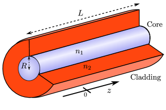
Figure 1: Illustration of the step-index circular waveguide geometry. The waveguide core with radius $R$ has a refractive index $n_{1}$ while the refractive index of the cladding layer is $n_{2}$. The total length of the waveguide is $L$.

III.1 Fields in a step-index circular waveguide

The electric and magnetic field modes are given as exact solutions of the Maxwell’s equations for the step-index circular waveguide geometry as presented, e.g., in Yariv2007 . These solutions are called Bessel modes. The necessary condition for the existence of confined modes is $n_{1}>n_{2}$. The cladding layer is assumed to be thick enough so that the field of confined modes is virtually zero in the outermost boundary of the cladding layer and we only need to account for the core and the cladding when computing the spatial distribution of the electromagnetic field inside the waveguide.

Here, we assume a light pulse with a nonzero spectral width as described by the Gaussian function $u(k_{0}^{\prime})=e^{-[(k_{0}^{\prime}-k_{0})/\Delta k_{0}]^{2}/2}/(\sqrt{2\pi}\Delta k_{0})$, where $k_{0}=\omega_{0}/c$ is the wavenumber in vacuum for central frequency $\omega_{0}$, and $\Delta k_{0}$ is the standard deviation of the wavenumber in vacuum. In the cylindrical coordinate system with coordinates $r$, $\phi$, and $z$ and basis vectors $\hat{\mathbf{r}}$, $\hat{\mathbf{\boldsymbol{\phi}}}$, and $\hat{\mathbf{z}}$, the instantaneous electric and magnetic fields of the Bessel mode pulses are given, in the waveguide core ($r<R$), as

$$\mathbf{E}_{\{r<R\}}(\mathbf{r},t)$$

$$=\mathrm{Re}\Big{(}\int_{-\infty}^{\infty}\Big{\{}\frac{ik_{z}^{\prime}}{h^{\prime 2}}\Big{[}Ah^{\prime}J_{l}^{\prime}(h^{\prime}r)+\frac{il\omega^{\prime}\mu_{0}}{k_{z}^{\prime}r}BJ_{l}(h^{\prime}r)\Big{]}\hat{\mathbf{r}}$$

$$\hskip 14.22636pt+\frac{ik_{z}^{\prime}}{h^{\prime 2}}\Big{[}\frac{il}{r}AJ_{l}(h^{\prime}r)-\frac{\omega^{\prime}\mu_{0}}{k_{z}^{\prime}}Bh^{\prime}J_{l}^{\prime}(h^{\prime}r)\Big{]}\hat{\boldsymbol{\phi}}$$

$$\hskip 14.22636pt+AJ_{l}(h^{\prime}r)\hat{\mathbf{z}}\Big{\}}e^{il\phi}u(k_{0}^{\prime})e^{i[k_{z}^{\prime}z-\omega(k_{z}^{\prime})t]}dk_{0}^{\prime}\Big{)},$$ (7)

$$\mathbf{H}_{\{r<R\}}(\mathbf{r},t)$$

$$=\mathrm{Re}\Big{(}\int_{-\infty}^{\infty}\Big{\{}\frac{ik_{z}^{\prime}}{h^{\prime 2}}\Big{[}Bh^{\prime}J_{l}^{\prime}(h^{\prime}r)-\frac{il\omega^{\prime}\varepsilon_{1}^{\prime}}{k_{z}^{\prime}r}AJ_{l}(h^{\prime}r)\Big{]}\hat{\mathbf{r}}$$

$$\hskip 14.22636pt+\frac{ik_{z}^{\prime}}{h^{\prime 2}}\Big{[}\frac{il}{r}BJ_{l}(h^{\prime}r)+\frac{\omega^{\prime}\varepsilon_{1}^{\prime}}{k_{z}^{\prime}}Ah^{\prime}J_{l}^{\prime}(h^{\prime}r)\Big{]}\hat{\boldsymbol{\phi}}$$

$$\hskip 14.22636pt+BJ_{l}(h^{\prime}r)\hat{\mathbf{z}}\Big{\}}e^{il\phi}u(k_{0}^{\prime})e^{i[k_{z}^{\prime}z-\omega(k_{z}^{\prime})t]}dk_{0}^{\prime}\Big{)},$$ (8)

and, in the cladding layer ($r>R$), as

$$\mathbf{E}_{\{r>R\}}(\mathbf{r},t)$$

$$=\mathrm{Re}\Big{(}\int_{-\infty}^{\infty}\Big{\{}-\frac{ik_{z}^{\prime}}{q^{\prime 2}}\Big{[}Cq^{\prime}K_{l}^{\prime}(q^{\prime}r)+\frac{il\omega^{\prime}\mu_{0}}{k_{z}^{\prime}r}DK_{l}(q^{\prime}r)\Big{]}\hat{\mathbf{r}}$$

$$\hskip 14.22636pt-\frac{ik_{z}^{\prime}}{q^{\prime 2}}\Big{[}\frac{il}{r}CK_{l}(q^{\prime}r)-\frac{\omega^{\prime}\mu_{0}}{k_{z}^{\prime}}Dq^{\prime}K_{l}^{\prime}(q^{\prime}r)\Big{]}\hat{\boldsymbol{\phi}}$$

$$\hskip 14.22636pt+CK_{l}(q^{\prime}r)\hat{\mathbf{z}}\Big{\}}e^{il\phi}u(k_{0}^{\prime})e^{i[k_{z}^{\prime}z-\omega(k_{z}^{\prime})t]}dk_{0}^{\prime}\Big{)},$$ (9)

$$\mathbf{H}_{\{r>R\}}(\mathbf{r},t)$$

$$=\mathrm{Re}\Big{(}\int_{-\infty}^{\infty}\Big{\{}-\frac{ik_{z}^{\prime}}{q^{\prime 2}}\Big{[}DqK_{l}^{\prime}(q^{\prime}r)-\frac{il\omega^{\prime}\varepsilon_{2}}{k_{z}^{\prime}r}CK_{l}(q^{\prime}r)\Big{]}\hat{\mathbf{r}}$$

$$\hskip 14.22636pt-\frac{ik_{z}^{\prime}}{q^{\prime 2}}\Big{[}\frac{il}{r}DK_{l}(q^{\prime}r)+\frac{\omega^{\prime}\varepsilon_{2}^{\prime}}{k_{z}^{\prime}}Cq^{\prime}K_{l}^{\prime}(q^{\prime}r)\Big{]}\hat{\boldsymbol{\phi}}$$

$$\hskip 14.22636pt+DK_{l}(q^{\prime}r)\hat{\mathbf{z}}\Big{\}}e^{il\phi}u(k_{0}^{\prime})e^{i[k_{z}^{\prime}z-\omega(k_{z}^{\prime})t]}dk_{0}^{\prime}\Big{)}.$$ (10)

Here $J_{l}(x)$ are the Bessel functions of the first kind, $K_{l}(x)$ are the modified Bessel functions of the second kind, $h=\sqrt{k_{1}^{2}-k_{z}^{2}}$, $q=\sqrt{k_{z}^{2}-k_{2}^{2}}$, and $\omega(k_{z}^{\prime})=ck_{z}^{\prime}/n_{\mathrm{p,eff}}^{\prime}$ is the waveguide dispersion relation with the effective phase index denoted by $n_{\mathrm{p,eff}}$ and the wavenumbers of the core and cladding are given by $k_{1}=n_{1}k_{0}$ and $k_{2}=n_{2}k_{0}$, respectively. The derivatives of the Bessel functions are denoted by $J_{l}^{\prime}(x)$ and $K_{l}^{\prime}(x)$. The other primed quantities in Eqs. (7)–(10) correspond to the values obtained for $k_{0}^{\prime}$ instead of $k_{0}$. The materials are here assumed to be nondispersive. The unknown amplitude factors $A$, $B$, $C$, and $D$ can be related to each other by applying the boundary conditions at the interface between the core and the cladding as described below or, e.g., in Yariv2007 .

In this work, we apply the fields above to describe the propagation of light pulses with a relatively small spectral width. In this limit, the light pulse is approximately monochromatic and Eqs. (7)–(10) can be approximated further in the same way as presented for Laguerre-Gaussian pulses in a homogeneous medium in Partanen2018a .

III.2 Characteristic equation and the relations between the field amplitudes

The unknown amplitude factors $A$, $B$, $C$, and $D$ can be related to each other by the boundary conditions. Requiring that $E_{\phi}$, $E_{z}$, $H_{\phi}$, and $H_{z}$ are continuous at the interface between the core and the cladding at $r=R$ leads to four equations, given by

$$AJ_{l}(hR)=CK_{l}(qR),$$ (11)

$$BJ_{l}(hR)=DK_{l}(qR),$$ (12)

$$A\frac{ilk_{z}}{\omega\mu_{0}R}\Big{(}\frac{1}{q^{2}}+\frac{1}{h^{2}}\Big{)}=B\Big{[}\frac{J_{l}^{\prime}(hR)}{hJ_{l}(hR)}+\frac{K_{l}^{\prime}(qR)}{qK_{l}(qR)}\Big{]},$$ (13)

$$A\Big{[}\frac{n_{1}^{2}J_{l}^{\prime}(hR)}{hJ_{l}(hR)}+\frac{n_{2}^{2}K_{l}^{\prime}(qR)}{qK_{l}(qR)}\Big{]}=B\frac{lk_{z}}{i\omega\varepsilon_{0}R}\Big{(}\frac{1}{q^{2}}+\frac{1}{h^{2}}\Big{)}.$$ (14)

Equations (13) and (14) lead to the characteristic equation for $k_{z}$ from which the coefficients $A$ and $B$ have been cancelled. This characteristic equation is transcendental and it reads

$$\Big{(}\frac{lk_{z}}{k_{0}R}\Big{)}^{2}\Big{(}\frac{1}{q^{2}}+\frac{1}{h^{2}}\Big{)}^{2}$$

$$=\Big{[}\frac{J_{l}^{\prime}(hR)}{hJ_{l}(hR)}+\frac{K_{l}^{\prime}(qR)}{qK_{l}(qR)}\Big{]}\Big{[}\frac{n_{1}^{2}J_{l}^{\prime}(hR)}{hJ_{l}(hR)}+\frac{n_{2}^{2}K_{l}^{\prime}(qR)}{qK_{l}(qR)}\Big{]}.$$ (15)

For a given $l$ and a given frequency $\omega$, there will be only a finite number of solutions $k_{z}$ that satisfy Eq. (15). Once a specific solution is known, one can use Eqs. (11)–(14) to solve the ratios of the amplitude factors $A$, $B$, $C$, and $D$. The absolute magnitudes of the amplitude factors become determined independent of a free phase factor by normalizing the fields so that the total electromagnetic energy of the light pulse is $E_{\mathrm{field}}$.

III.3 Waveguide dispersion

The effective phase refractive index $n_{\mathrm{p,eff}}$ for the field propagating in the optical fiber is given as the ratio of $k_{z}$, solved from the characteristic equation in Eq. (15), and $k_{0}$ as Yariv2007

$$n_{\mathrm{p,eff}}=\frac{k_{z}}{k_{0}}.$$ (16)

In terms of the total MP momentum in Eq. (5) and the field energy in Eq. (4), the effective phase refractive index can also be written as $n_{\mathrm{p,eff}}=c|\mathbf{P}_{\mathrm{MP}}|/E_{\mathrm{field}}$. This relation is justified by the numerical OCD simulations of Sec. IV. From the characteristic equation, one also obtains the effective group refractive index $n_{\mathrm{g,eff}}$, given by

$$n_{\mathrm{g,eff}}=\frac{\partial k_{z}}{\partial k_{0}}.$$ (17)

There also exists an alternative well-known expression for the group refractive index as a ratio of the integrals of the energy density and the Poynting vector. Using Eqs. (4) and (5), we then obtain $n_{\mathrm{g,eff}}=E_{\mathrm{field}}/(c|\mathbf{P}_{\mathrm{field}}|)$.

III.4 Field modes and cutoff conditions

III.4.1 TE and TM modes

First, we consider the special cases of the $TE$ and $TM$ modes. For the $TE$ modes, we have $E_{z}=0$, from which it follows that $A=C=0$. In this case, the left hand sides of Eqs. (13) and (14) become zero. Equation (14) is then satisfied if $l=0$ and Eq. (13) leads to the characteristic equation for the $TE$ modes given by

$$\frac{J_{1}(hR)}{hRJ_{0}(hR)}=-\frac{K_{1}(qR)}{qRK_{0}(qR)},$$ (18)

where we have used the Bessel function relations $J_{0}^{\prime}(x)=-J_{1}(x)$ and $K_{0}^{\prime}(x)=-K_{1}(x)$. The remaining Eq. (11) is trivially satisfied and Eq. (12) relates the nonzero field amplitudes $B$ and $D$ to each other.

Respectively, for the $TM$ modes we have $H_{z}=0$, from which it follows that $B=D=0$. In this case, the right hand sides of Eqs. (13) and (14) become zero. Equation (13) is then satisfied if $l=0$ and Eq. (14) leads to the characteristic equation for the $TM$ modes given by

$$\frac{J_{1}(hR)}{hRJ_{0}(hR)}=-\frac{n_{2}^{2}K_{1}(qR)}{n_{1}^{2}qRK_{0}(qR)},$$ (19)

where we have again used the Bessel function relations $J_{0}^{\prime}(x)=-J_{1}(x)$ and $K_{0}^{\prime}(x)=-K_{1}(x)$. The remaining Eq. (12) is trivially satisfied and Eq. (11) relates the nonzero field amplitudes $A$ and $C$ to each other.

The $TE_{0,m}$ and $TM_{0,m}$ modes are numbered so that the lowest mode number $m$ corresponds to the solution of the characteristic equation for which the value of $hR$ is the smallest. The cutoff condition for the existence of the $TE_{0,m}$ and $TM_{0,m}$ modes is given by Yariv2007

$$\Big{(}\frac{R}{\lambda_{0}}\Big{)}_{0,m}\geq\frac{x_{0,m}}{2\pi\sqrt{n_{1}^{2}-n_{2}^{2}}},$$ (20)

where $x_{0,m}$, $m\geq 1$, is the $m$th zero of the Bessel function $J_{0}(x)$. The first three zeros of the Bessel function $J_{0}(x)$ are $x_{0,1}=2.405$, $x_{0,2}=5.520$, and $x_{0,3}=8.654$.

III.4.2 EH and HE modes

Second, we consider the general solution of the characteristic equation in Eq. (15). Solving the characteristic equation for $J_{l}^{\prime}(hR)/(hRJ_{l}(hR))$ gives

$$\frac{J_{l}^{\prime}(hR)}{hRJ_{l}(hR)}$$

$$=-\Big{(}\frac{n_{1}^{2}+n_{2}^{2}}{2n_{1}^{2}}\Big{)}\frac{K_{l}^{\prime}(qR)}{qRK_{l}(qR)}\pm\Big{[}\Big{(}\frac{n_{1}^{2}-n_{2}^{2}}{2n_{1}^{2}}\Big{)}^{2}\Big{(}\frac{K_{l}^{\prime}(qR)}{qRK_{l}(qR)}\Big{)}^{2}$$

$$\hskip 14.22636pt+\Big{(}\frac{lk_{z}}{n_{1}k_{0}}\Big{)}^{2}\Big{(}\frac{1}{(qR)^{2}}+\frac{1}{(hR)^{2}}\Big{)}^{2}\Big{]}^{1/2}.$$ (21)

Here, the plus sign corresponds to the $EH$ modes and the minus sign corresponds to the $HE$ modes. The cutoff conditions for the existence of the $EH_{1,m}$ and $HE_{1,m}$ modes are given by Yariv2007

$$\Big{(}\frac{R}{\lambda_{0}}\Big{)}_{1,m}^{EH}\geq\frac{x_{1,m}}{2\pi\sqrt{n_{1}^{2}-n_{2}^{2}}},\hskip 8.5359pt\Big{(}\frac{R}{\lambda_{0}}\Big{)}_{1,m}^{HE}\geq\frac{x_{1,m-1}}{2\pi\sqrt{n_{1}^{2}-n_{2}^{2}}},$$ (22)

where $x_{1,m}$, $m\geq 1$, is the $m$th zero of the Bessel function $J_{1}(x)$ and $x_{1,0}=0$. The first three zeros of the Bessel function $J_{1}(x)$ are $x_{1,1}=3.832$, $x_{1,2}=7.016$, and $x_{1,3}=10.173$. The cutoff values of $(R/\lambda_{0})_{1,m}$ for the $HE_{1,m}$ modes are smaller than for the $EH_{1,m}$ modes, and especially, the mode $HE_{1,1}$ does not have a cutoff. The cutoff conditions for the existence of the $EH_{l,m}$ and $HE_{l,m}$ modes with $l\geq 2$ are given by Yariv2007

$$\Big{(}\frac{R}{\lambda_{0}}\Big{)}_{l,m}^{EH}\geq\frac{x_{l,m}}{2\pi\sqrt{n_{1}^{2}-n_{2}^{2}}},\hskip 8.5359pt\Big{(}\frac{R}{\lambda_{0}}\Big{)}_{l,m}^{HE}\geq\frac{z_{l,m}}{2\pi\sqrt{n_{1}^{2}-n_{2}^{2}}},$$ (23)

where $x_{l,m}$, $m\geq 1$, is the $m$th zero of the Bessel function $J_{l}(x)$ and $z_{l,m}$ is the $m$th root of equation $zJ_{l}(z)=(l-1)(1+n_{1}^{2}/n_{2}^{2})J_{l-1}(z)$.

III.5 Angular momentum and relation to Laguerre-Gaussian modes

The Bessel modes studied in this work are eigenmodes of step-index circular waveguides as discussed above. The step-index profile is used in most single-mode fibers and in some multi-mode fibers. In counter distinction, Laguerre-Gaussian modes are eigenmodes of graded-index circular waveguides with a parabolic refractive index profile. The parabolic profile is the most common profile in graded-index multi-mode fibers as it minimizes modal dispersion by continual refocusing of the rays in the fiber core. The Bessel and Laguerre-Gaussian beams can both carry angular momentum. This has been experimentally demonstrated by rotating microparticles in optical tweezers Grier2003 ; He1995 ; Friese1996 ; Simpson1997 ; Friese1998 ; ONeil2002 ; CarcesChavez2003 ; Adachi2007 .

IV Simulations

Next, we apply the OCD model to illustrate the node structure of the atomic MDW and the actual atomic displacements due to a light pulse in a circular waveguide made of fused silica. The light pulse of Eqs. (7)–(10) is assumed to have a total electromagnetic energy of $U_{0}=1$ $\mu$J and a vacuum wavelength of $\lambda_{0}=1550$ nm. The corresponding photon number is $N_{\mathrm{ph}}=E_{\mathrm{field}}/\hbar\omega_{0}=7.803\times 10^{12}$. In our examples, the waveguide core radius is $R=\lambda_{0}/2$. The relative spectral width of the pulse used in the simulations is $\Delta\omega/\omega_{0}=\Delta k_{0}/k_{0}=0.05$, which corresponds to the temporal full width at half maximum (FWHM) of $\Delta t_{\mathrm{FWHM}}=27$ fs. The FWHM is fixed to this small value, which is close to the engineering feasibility limit, to make the node structure of the MDW visible in the same scale with the longitudinal Gaussian envelope of the pulse. In our simulations, we use temporal discretization of $h_{t}=2\pi/(40\omega_{0})$ and spatial discretization of $h_{z}=\lambda/40$, where $\lambda=\lambda_{0}/n_{\mathrm{p,eff}}$ is the effective wavelength of the studied mode in the waveguide. This discretization is sufficiently dense compared to the scale of the harmonic cycle of the optical field. The flowchart of the OCD simulation is described in Appendix C of Partanen2017c .

The simulations are performed for a waveguide whose core is assumed to be made of fused silica, which is the standard material used in optical fibers. The cladding layer is assumed to be vacuum meaning that there is no cladding. The corresponding fields are a special case of Eqs. (7)–(10) obtained by setting $n_{2}=1$. The phase and group refractive indices of fused silica are given by $n_{\mathrm{p}}=1.4440$, and $n_{\mathrm{g}}=1.4626$ for $\lambda_{0}=1550$ nm Malitson1965 . As the material dispersion is not very large, in this work, we neglect the material dispersion and use the phase refractive index only. However, the material dispersion could be accounted for as explained in Partanen2017e . The waveguide dispersion is here the dominating form of dispersion and it is described by the effective phase and group refractive indices of the waveguide geometry following from Eqs. (16) and (17). For the $TE_{0,1}$ mode studied below, the effective phase refractive index of our waveguide geometry is $n_{\mathrm{p,eff}}=1.1330$ and the effective group refractive index is $n_{\mathrm{g,eff}}=1.5856$. Respectively, for the $HE_{1,1}$ mode that is studied in the second example, the effective phase refractive index is $n_{\mathrm{p,eff}}=1.3033$ and the effective group refractive index is $n_{\mathrm{g,eff}}=1.5355$. The mass density of fused silica used in the OCD simulations is $\rho_{0}=2200$ kg/m³ Bruckner1970 , and the Lamé elastic constants are $\lambda_{\mathrm{L}}=15.4$ GPa and $\mu_{\mathrm{L}}=31.3$ GPa DeJong2000 .

IV.1 Simulations of the atomic mass density wave

First, we study the atomic MDW of a temporally Gaussian $TE_{0,1}$ light pulse for which $l=0$. See Visualization 1 for a video file of the simulation. Figure 2(a) shows the longitudinal atomic velocities of the simulated MDW as a function of position in the plane $y=0$ $\mu$m when the $TE_{0,1}$ pulse center is propagating at the position $z=0$ $\mu$m. In vacuum, outside the waveguide core at $x<-\lambda_{0}/2$ or at $x>\lambda_{0}/2$, the atomic velocities are zero as the atomic MDW does not exist. Inside the waveguide core, the atomic velocities in the MDW follow the field intensity. The node structure of the field is then also well seen in the atomic MDW. The atomic velocities are zero at the center of the waveguide at the position $x=0$ $\mu$m following the $TE_{0,1}$ mode profile. When the Gaussian envelope of the pulse drops to zero on the left of $z=-5$ $\mu$m and on the right of $z=5$ $\mu$m, also the atomic velocities of the MDW become zero.

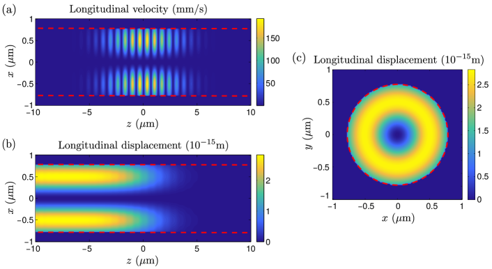
Figure 2: Simulation of the mass transfer due to a temporally Gaussian $TE_{0,1}$ mode light pulse in a silica fiber (see also Visualization 1). (a) Simulated longitudinal atomic velocity of the MDW in the fiber as a function of position in the plane $y=0$ $\mu$m. (b) Longitudinal atomic displacement in the fiber as a function of position in the plane $y=0$ $\mu$m. (c) Longitudinal atomic displacement in the fiber cross section $z=0$ $\mu$m just after the pulse has gone. The pulse energy is $E_{\mathrm{field}}=1$ $\mu$J, the wavelength is $\lambda_{0}=1550$ nm, and the duration is $\Delta t_{\mathrm{FWHM}}=27$ fs. The radius of the circular fiber core is $R=\lambda_{0}/2$ and it is surrounded by vacuum. The dashed line shows the boundaries of the fiber.

Figure 2(b) shows the longitudinal atomic displacements of the simulated MDW as a function of position along $z$ axis in the plane $y=0$ $\mu$m when the $TE_{0,1}$ pulse center is propagating at the position $z=0$ $\mu$m corresponding to the atomic velocities in Fig. 2(a). One can see that the atomic displacements are largest at lateral positions of maximum field intensity. At positions $z>5$ $\mu$m, the atomic displacement is zero as the light pulse has not yet reached these positions, and therefore, these atoms have not yet experienced the optical force density. In vacuum, outside the waveguide core, the atomic displacement in Fig. 2(b) is zero as the atomic velocities in Fig. 2(a). Behind the light pulse at $z<-5$ $\mu$m, the atomic displacement has obtained a value that is in the femtosecond time scale practically constant in time, but which varies in the lateral direction. This atomic displacement is also the origin of the transferred mass of the MDW and the corresponding mass energy term in Eq. (4) since it is related to the denser spacing of atoms at the position of the light pulse.

The longitudinal atomic displacement in the waveguide cross section just after the light pulse has gone is presented in Fig. 2(c). These atomic displacements correspond to the atomic displacements behind the light pulse in Fig. 2(b). The atomic displacement averaged over the waveguide cross section is given by $\Delta r_{\mathrm{MDW}}=\delta M/(\rho_{0}\pi R^{2})=2.135\times 10^{-15}$ m. The atomic displacements that the light pulse leaves behind are relaxed to equilibrium only in the much larger time scale of elastic waves. The relaxation dynamics of the waveguide in the longer time scale is studied in more detail in Sec. IV.2.

The OCD simulation results in Fig. 2 are fully consistent with the MP quasiparticle model of Partanen2017c ; Partanen2017e as the total transferred mass and momentum following from the atomic velocities and displacements equal the quasiparticle model results within the 6-digit numerical accuracy of the simulation. This very good accuracy is related to the monochromatic field approximation of light pulses used in the OCD simulations. It is not exact for our short pulses, but the relative error is found to be less than 1%, which is sufficient for our visualization purposes. Therefore, our results must be interpreted to indicate that full agreement between the OCD and MP quasiparticle models is obtained in the limit of long narrow-band pulses in which limit our pulse approximation becomes exact. For the total transferred mass, the MP quasiparticle model gives an expression $\delta M=(n_{\mathrm{p,eff}}n_{\mathrm{g,eff}}-1)N_{\mathrm{ph}}\hbar\omega_{0}/c^{2}$ that is obtained from the homogeneous field result presented in Partanen2017e by simply replacing the phase and group refractive indices of the material with the conventional effective values for the studied mode in the waveguide geometry. The numerical OCD model gives the total transferred mass for our $TE_{0,1}$ mode light pulse as $\delta M=\int[\rho_{\mathrm{a}}(\mathbf{r},t)-\rho_{0}]d^{3}r=8.862\times 10^{-24}$ kg, which corresponds to the value obtained by using the MP quasiparticle model formula. For the momentum of the MDW, the OCD simulations give $p_{\mathrm{MDW}}=|\int\rho_{\mathrm{a}}(\mathbf{r},t)\mathbf{v}_{\mathrm{a}}(\mathbf{r},t)d^{3}r|=1.676\times 10^{-15}$ kgm/s, which corresponds to the MP quasiparticle model value obtained by using $p_{\mathrm{MDW}}=(n_{\mathrm{g,eff}}-1/n_{\mathrm{g,eff}})N_{\mathrm{ph}}\hbar\omega_{0}/c$.

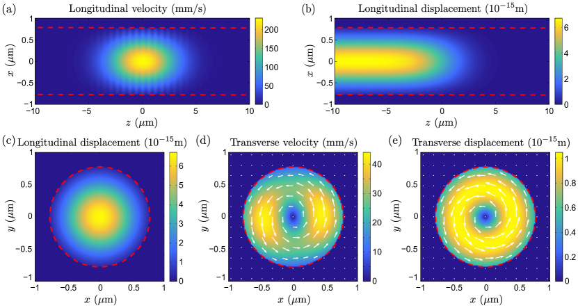
Figure 3: Simulation of the mass transfer due to a temporally Gaussian $HE_{1,1}$ mode light pulse in a silica fiber (see also Visualization 2). (a) Longitudinal atomic velocity of the MDW in the fiber as a function of position in the plane $y=0$ $\mu$m. (b) Longitudinal atomic displacement in the fiber as a function of position in the plane $y=0$ $\mu$m. (c) Longitudinal atomic displacement in the fiber cross section $z=0$ $\mu$m just after the pulse has gone. (d) Instantaneous transverse atomic velocity of the MDW in the fiber as a function of position in the fiber cross section at the position of the pulse center at $z=0$ $\mu$m. (e) Transverse atomic displacement in the fiber as a function of position in the fiber cross section $z=0$ $\mu$m just after the light pulse has gone. The pulse energy is $E_{\mathrm{field}}=1$ $\mu$J, the wavelength is $\lambda_{0}=1550$ nm, and the duration is $\Delta t_{\mathrm{FWHM}}=27$ fs. The radius of the circular fiber core is $R=\lambda_{0}/2$ and it is surrounded by vacuum. The dashed line shows the boundaries of the fiber.

Another interesting case is the $HE_{1,1}$ mode light pulse for which $l=1$. This pulse does not have a cutoff, and in contrast to the $TE_{0,1}$ pulse above, it carries angular momentum of $\hbar$ per photon. See Visualization 2 for a video file of the simulation. Figure 3(a) depicts the atomic velocities of the simulated MDW as a function of position in the plane $y=0$ $\mu$m when the $HE_{1,1}$ pulse center is propagating at the position $z=0$ $\mu$m. Inside the waveguide core, the atomic velocities in the MDW again follow the field intensity. As the $HE_{1,1}$ mode is not a transverse mode, the pulse does not have as clear peaks and throughs as the $TE_{0,1}$ pulse above. Also, in contrast to the $TE_{0,1}$ pulse, the atomic velocities obtain their maximum values at the center of the waveguide at the position $x=0$ $\mu$m in accordance with the $HE_{1,1}$ mode profile. On the left and right of the light pulse, the atomic velocities in the MDW are again zero as expected.

Figure 3(b) depicts the longitudinal atomic displacements of the simulated MDW as a function of position along $z$ axis in the plane $y=0$ $\mu$m when the $HE_{1,1}$ pulse center is propagating at the position $z=0$ $\mu$m. These atomic displacements correspond to the atomic velocities in Fig. 3(a). One can again see that the longitudinal atomic displacements are largest at lateral positions of maximum field intensity. In front of the light pulse at positions $z>5$ $\mu$m, the atomic displacement is again zero and, behind the light pulse at $z<-5$ $\mu$m, the atomic displacement has obtained a value that is temporally approximatively constant in the femtosecond time scale. The longitudinal atomic displacements of the $HE_{1,1}$ pulse just after the light pulse has gone is presented in the waveguide cross section in Fig. 3(c). These atomic displacements correspond to the atomic displacements after the light pulse in Fig. 3(b). The atomic displacement averaged over the waveguide cross section is given by $\Delta r_{\mathrm{MDW}}=\delta M/(\rho_{0}\pi R^{2})=2.683\times 10^{-15}$ m.

The simulation results are again in full correspondence with the MP quasiparticle model of Partanen2017c and Partanen2017e . Again, note that full agreement is obtained by using the monochromatic field approximation of light pulses in the OCD model. For the total transferred mass of our $HE_{1,1}$ pulse, we obtain $\delta M=1.114\times 10^{-23}$ kg and, for the momentum of the MDW, we obtain a value $p_{\mathrm{MDW}}=2.175\times 10^{-15}$ kgm/s. These values are slightly larger than the values in the case of the $TE_{0,1}$ pulse due to the smaller evanescent field that propagates in vacuum outside the fiber core and that does not directly contribute to the atomic MDW. In the MP quasiparticle model, this difference between the quantities is accounted for by the effective phase and group refractive indices of the waveguide corresponding to the somewhat smaller waveguide dispersion in the $HE_{1,1}$ case.

Figure 3(d) presents the transverse components of the atomic velocities in the MDW at a particular instance of time in the middle of the $HE_{1,1}$ light pulse. The transverse components of the atomic velocities follow from the nonzero transverse components of the optical force density and the Poynting vector, which do not exist in the case of the $TE_{0,1}$ pulse above. As described in Partanen2018a , the transverse components of the atomic velocities are related to the transfer of a substantial part of the total angular momentum of light in a medium. The angular momentum of the electromagnetic field of the $HE_{1,1}$ pulse obtained using the OCD model is $\mathbf{J}_{\mathrm{field}}=0.586N_{\mathrm{ph}}\hbar\hat{\mathbf{z}}$ and the angular momentum of the MDW is $\mathbf{J}_{\mathrm{MDW}}=0.414N_{\mathrm{ph}}\hbar\hat{\mathbf{z}}$. The sum of these angular momentum contributions is the total angular momentum of the coupled state of the field and matter, given by $\mathbf{J}_{\mathrm{MP}}=N_{\mathrm{ph}}\hbar\hat{\mathbf{z}}$, which is essentially an integer multiple of $\hbar$. This result verifies the coupling of the field and medium components of the total angular momentum of a light pulse in the case of a waveguide geometry. Previously, this coupling has been studied in the case of a homogeneous medium in Partanen2018a .

The cross section of the total transverse atomic displacement field that the $HE_{1,1}$ pulse leaves behind, and which follows from the transverse atomic velocities in Fig. 3(d), is depicted in Fig. 3(e). Together with the longitudinal atomic displacements in Fig. 3, these transverse atomic displacements are again relaxed to equilibrium in the time scale of elastic waves.

IV.2 Simulations of the elastic relaxation dynamics

In the OCD simulations, the optical force density of the light pulse displaces atoms from their initial equilibrium positions by different amounts in the cross section of the fiber. Therefore, there will be strain and related elastic forces acting between atoms after the light pulse has gone and when, accordingly, the optical force is zero. Thus, the after-the-light-pulse elastic relaxation dynamics is a novel feature of the OCD model that results from rejecting the approximation of fixed atoms. In this work, we simulate the elastic relaxation of the medium by using elasticity theory without including terms that lead to thermalization. The elastic relaxation dynamics has been previously simulated in the case of a homogeneous material block in Partanen2017c and it has been qualitatively described in the case of optical fibers in Partanen2017e .

Here, we simulate the beginning of the relaxation of the nonequilibrium atomic displacements of the waveguide after the $TE_{0,1}$ light pulse of Fig. 2 has gone. The initial atomic displacement for this relaxation process is that presented in Fig. 2(c). We assume that the fiber is infinitely long, which is realized in the simulations by setting periodic boundary conditions in the longitudinal direction just after the light pulse has gone. The damping of the elastic waves in a closed system is not accounted for by the elastic force density in Eq. (3). Therefore, the elastic waves that we obtain do not attenuate. Hence, we cannot simulate how the equilibrium of atomic positions is obtained at the end of the relaxation. Instead, we focus on the first nanosecond when the damping of the elastic waves can be neglected.

Figure 4 presents the relaxation dynamics of the waveguide after the $TE_{0,1}$ light pulse of Fig. 2 has gone. It shows the longitudinal atomic displacement in the waveguide cross section at three instances of time in the picosecond time scale. See Visualization 3 for a video file of the simulation. Figure 4(a) shows the longitudinal atomic displacement at $t=110$ ps, Fig. 4(b) at $t=200$ ps, and Fig. 4(c) at $t=260$ ps. One can see that the minima and maxima of the atomic displacement switch their positions in the course of time. In Figs. 4(a) and 4(c), the maximum atomic displacement is located at the origin while, in Fig. 4(b), at the origin, the atomic displacement obtains its minimum value. This can be understood as elastic shear waves that propagate from the circular fiber boundary to the center and back. The atomic displacement minima and maxima alternate, but their time-evolution is not fully periodic since the initial state of the relaxation process is not an eigenstate of the elastic oscillation of the waveguide.

Figure 4(d) shows the kinetic and strain energies of the elastic relaxation waves per unit length of the fiber as a function of time. At $t=0$, the elastic energy is pure strain energy as the light pulse has only displaced atoms from their initial equilibrium positions but does not have left any net kinetic energy to them. At $t>0$, the kinetic and strain energies alternate as a function of time so that their sum remains constant due to the conservation of energy. The highest peaks and throughs in the kinetic and strain energies at $t=413$ ps and $t=826$ ps are seen to be located close to times at which the shear waves with velocity $v_{\perp}=\sqrt{\mu_{\mathrm{L}}/\rho_{0}}=3770$ m/s have propagated distances that are multiples of the waveguide diameter.

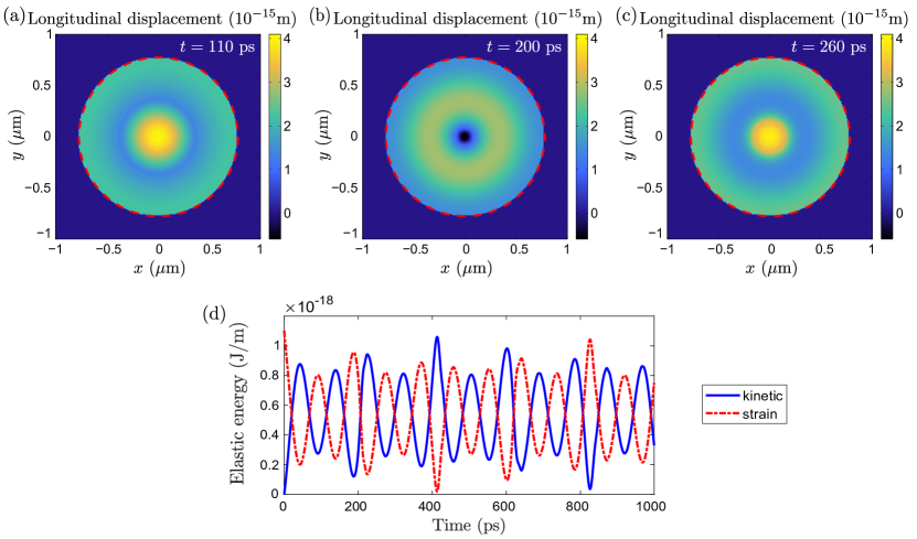
Figure 4: Simulation of the elastic relaxation dynamics of the silica waveguide after the $TE_{0,1}$ mode light pulse (see also Visualization 3). The pulse energy is $E_{\mathrm{field}}=1$ $\mu$J, the wavelength is $\lambda_{0}=1550$ nm, and $\Delta t_{\mathrm{FWHM}}=27$ fs. Longitudinal atomic velocity of the MDW at $z=0$ $\mu$m cross section is shown at (a) $t=110$ ps, (b) $t=200$ ps, and (c) $t=260$ ps after the pulse has gone. The radius of the circular fiber core is $R=\lambda_{0}/2$ and it is surrounded by vacuum. The dashed line shows the fiber boundary. (d) The alternation of the elastic (kinetic and strain) energies per unit length of the fiber as a function of time. The elastic waves are gradually damped and thermalized by absorption and scattering not included in our simulations. Due to the periodic boundary conditions used in the simulation of the elastic relaxation, the interface effects at the ends of the fiber are not present.

The value of the total elastic energy, left in the waveguide after the light pulse has gone, can be used to estimate the effective imaginary part of the refractive index $n_{\mathrm{i}}$, which corresponds to the dissipation of the field energy when the field propagates in the waveguide. The total elastic energy left in the waveguide per unit length is $1.1\times 10^{-18}$ J/m as can be read from Fig. 4(d). Dividing this dissipated energy by the field energy $U_{0}$ of the pulse, gives the attenuation coefficient $1.1\times 10^{-12}$ 1/m. When this value is compared with the conventional formula for the attenuation coefficient, given by $\alpha=2n_{\mathrm{i}}k_{0}$, we obtain $n_{\mathrm{i}}=1.4\times 10^{-19}$. This is vastly smaller than the imaginary part of the refractive index due to other physical nonidealities in highly transparent optical waveguides that are not accounted for in the present simulations.

All of the elastic strain energy that is left in the crystal after the light pulse has gone will be converted into heat in the course of time. The detailed simulation of the thermalization of strain is beyond the scope of the present manuscript. The dissipation of field energy into energy of elastic waves is an additional very small loss mechanism to the dominant losses in realistic transparent materials. We find the MDW-related dissipation effect even though we initially assume that the refractive index is real valued and the field is not damped. In self-consistent calculations, the corresponding damping of the field could be accounted for through the self-consistently determined value of the imaginary part of the refractive index. Note, however, that the self-consistent calculations accounting for the imaginary part of the refractive index coming from the elastic MDW losses alone are not meaningful as this extremely small imaginary part refers to damping that is several orders of magnitude smaller than the total damping in the best transparent solids.

Since the velocity of light is vastly larger than the velocity of sound, the relaxation process practically starts only after our short light pulse has gone. In this approximation, during the relaxation process, the total external force on the medium atoms is zero. Therefore, in accordance with Newton’s first law, the center of mass of the waveguide remains at rest during the relaxation process since the light pulse has only displaced atoms from their initial equilibrium positions but does not have left any net kinetic energy to them as discussed above. This contrasts to the state of motion of the waveguide under the influence of the optical force of the light pulse, which moves the center of mass of the waveguide slightly forwards by the atomic MDW that is present in the waveguide while the light pulse is propagating in it.

The same kind of relaxation waves, as obtained for the longitudinal atomic displacements in Fig. 4, are also obtained for the transverse atomic displacements in the relaxation of the atomic displacements due to optical modes carrying angular momentum. These waves are also elastic shear waves in nature. Compressional waves are not obtained as the light pulse does not leave any mass density differences behind in the middle of the waveguide. As shown in Partanen2017c , compressional waves are found in the case that a light pulse crosses an interface between materials of different refractive indices. Then, the optical surface force displaces atoms at the surface and these displacements are relaxed in terms of both compressional and shear waves. In the case of optical fibers, compressional waves can originate from the processes at the ends of the fiber or at any positions where there are changes in the refractive index.

V Comparison of the OCD and MP quasiparticle models

The correspondence between the OCD and MP quasiparticle model results is summarized in Table 1. Full agreement is obtained within the numerical accuracy of the simulations and the monochromatic field approximation of light pulses used in the OCD model. The results for the energy and momentum of the MP and its field and medium parts are identical to the results for a homogeneous medium in Partanen2017c with an exception that we must now use the effective phase and group refractive indices of the waveguide in the MP quasiparticle model. Consequently, we obtain the ratio $n_{\mathrm{p,eff}}n_{\mathrm{g,eff}}-1$ for the MDW’s and the electromagnetic field’s shares of energies and momenta. This result is directly related to the Lorentz transformation and the covariance principle of the special theory of relativity in the same way as described in the case of a homogeneous medium in Partanen2017c .

Also, note that many previous works, which are not directly related to the MP theory of light, obtain the Minkowski momentum as the total momentum of light Barnett2010b ; Bliokh2017a ; Bliokh2017b ; Leonhardt2014 ; Brevik2017 in agreement with our result in Table 1. Since these works are typically based on the approximation of fixed atoms, they are not able to unambiguously separate the total momentum of light between the field and the atoms. In the work of Leonhardt Leonhardt2014 , the atoms are allowed to move, but the medium is assumed to be incompressible, which effectively makes one to neglect the coupled field-medium dynamics studied in the present work.

Table 1: The transferred mass, the total momentum, the field’s share of the momentum, and the MDW’s share of the momentum calculated by using the MP and OCD models. The MP column shows the per photon value obtained by dividing the total quantities of the MP model with the photon number of the pulse $N_{\mathrm{ph}}=E_{\mathrm{field}}/\hbar\omega_{0}$.

	OCD	MP
$\delta M$	$\displaystyle\int\rho_{\mathrm{MDW}}d^{3}r$	$\displaystyle(n_{\mathrm{p,eff}}n_{\mathrm{g,eff}}-1)\frac{\hbar\omega_{0}}{c^{2}}$
$\mathbf{P}_{\mathrm{MP}}$	$\displaystyle\int\Big{(}\rho_{\mathrm{a}}\mathbf{v}_{\mathrm{a}}+\frac{\mathbf{E}\times\mathbf{H}}{c^{2}}\Big{)}d^{3}r$	$\displaystyle\frac{n_{\mathrm{p,eff}}\hbar\omega_{0}}{c}\hat{\mathbf{z}}$
$\mathbf{P}_{\mathrm{field}}$	$\displaystyle\int\frac{\mathbf{E}\times\mathbf{H}}{c^{2}}d^{3}r$	$\displaystyle\frac{\hbar\omega_{0}}{n_{\mathrm{g,eff}}c}\hat{\mathbf{z}}$
$\mathbf{P}_{\text{MDW}}$	$\displaystyle\int\rho_{\mathrm{a}}\mathbf{v}_{\mathrm{a}}d^{3}r$	$\displaystyle\Big{(}n_{\mathrm{p,eff}}-\frac{1}{n_{\mathrm{g,eff}}}\Big{)}\frac{\hbar\omega_{0}}{c}\hat{\mathbf{z}}$
$\mathbf{J}_{\mathrm{MP}}$	$\displaystyle\int\mathbf{r}\times\Big{(}\rho_{\mathrm{a}}\mathbf{v}_{\mathrm{a}}+\frac{\mathbf{E}\times\mathbf{H}}{c^{2}}\Big{)}d^{3}r$	$l\hbar\hat{\mathbf{z}}$
$\mathbf{J}_{\mathrm{field}}$	$\displaystyle\int\mathbf{r}\times\Big{(}\frac{\mathbf{E}\times\mathbf{H}}{c^{2}}\Big{)}d^{3}r$	$\displaystyle\zeta l\hbar\hat{\mathbf{z}}$
$\mathbf{J}_{\mathrm{MDW}}$	$\displaystyle\int\mathbf{r}\times\rho_{\mathrm{a}}\mathbf{v}_{\mathrm{a}}d^{3}r$	$\displaystyle(1-\zeta)l\hbar\hat{\mathbf{z}}$

The waveguide dispersion also influences the separation of the total angular momentum of light between the field and matter as described by the parameter $\zeta=|\mathbf{J}_{\mathrm{field}}|/|\mathbf{J}_{\mathrm{MP}}|$ used in Table 1. Analytic calculation using Eq. (6) and the fields in Eqs. (7)–(10) shows that the angular momenta of the field and the MDW are given by

$$|\mathbf{J}_{\mathrm{field}}| =\frac{\pi^{3/2}k_{0}R^{2}}{cn_{\mathrm{g,eff}}\Delta k_{0}h^{2}}\Big{\{}\frac{l}{2}\Big{(}\varepsilon_{1}|A|^{2}+\mu_{0}|B|^{2}\Big{)}$$

$$\hskip 11.38092pt\times\Big{[}J_{l}(Rh)^{2}-J_{l-1}(Rh)J_{l+1}(Rh)\Big{]}$$

$$\hskip 11.38092pt+\mathrm{sign}(l)\frac{n_{\mathrm{p,eff}}}{c}|AB|J_{l-1}(Rh)J_{l+1}(Rh)\Big{\}}$$

$$\hskip 11.38092pt+\frac{\pi^{3/2}k_{0}R^{2}}{cn_{\mathrm{g,eff}}\Delta k_{0}q^{2}}\Big{\{}\frac{l}{2}\Big{(}\varepsilon_{2}|C|^{2}+\mu_{0}|D|^{2}\Big{)}$$

$$\hskip 11.38092pt\times\Big{[}K_{l}(Rq)^{2}-K_{l-1}(Rq)K_{l+1}(Rq)\Big{]}$$

$$\hskip 11.38092pt+\mathrm{sign}(l)\frac{n_{\mathrm{p,eff}}}{c}|CD|K_{l-1}(Rq)K_{l+1}(Rq)\Big{\}},$$ (24)

$$|\mathbf{J}_{\mathrm{MDW}}| =\frac{(n_{1}^{2}-1)\pi^{3/2}k_{0}R^{2}}{cn_{\mathrm{g,eff}}\Delta k_{0}h^{2}}\Big{\{}\frac{l}{2}\Big{(}\varepsilon_{1}|A|^{2}+\mu_{0}|B|^{2}\Big{)}$$

$$\hskip 11.38092pt\times\Big{[}J_{l}(Rh)^{2}-J_{l-1}(Rh)J_{l+1}(Rh)\Big{]}$$

$$\hskip 11.38092pt+\mathrm{sign}(l)\frac{n_{\mathrm{p,eff}}}{c}|AB|J_{l-1}(Rh)J_{l+1}(Rh)\Big{\}}$$

$$\hskip 11.38092pt+\frac{(n_{2}^{2}-1)\pi^{3/2}k_{0}R^{2}}{cn_{\mathrm{g,eff}}\Delta k_{0}q^{2}}\Big{\{}\frac{l}{2}\Big{(}\varepsilon_{2}|C|^{2}+\mu_{0}|D|^{2}\Big{)}$$

$$\hskip 11.38092pt\times\Big{[}K_{l}(Rq)^{2}-K_{l-1}(Rq)K_{l+1}(Rq)\Big{]}$$

$$\hskip 11.38092pt+\mathrm{sign}(l)\frac{n_{\mathrm{p,eff}}}{c}|CD|K_{l-1}(Rq)K_{l+1}(Rq)\Big{\}}.$$ (25)

Therefore, using $|\mathbf{J}_{\mathrm{MP}}|=|\mathbf{J}_{\mathrm{field}}|+|\mathbf{J}_{\mathrm{MDW}}|$ one also obtains an analytic expression for the parameter $\zeta=|\mathbf{J}_{\mathrm{field}}|/|\mathbf{J}_{\mathrm{MP}}|$. In the case of a homogeneous medium with a refractive index $n$, we have $\zeta=1/n^{2}$ as shown in Partanen2018a . In contrast, in the waveguide geometry studied in this work, we have not found a simple expression for $\zeta$ in terms of the effective phase and group refractive indices of the waveguide. One can argue that this is not surprising as the covariance condition of the special theory of relativity used in the MP quasiparticle model relates the energies and momenta of the field and the MDW to each other Partanen2017c but no such a simple quasiparticle model relation is known to exist for the separation of angular momentum. In the case of angular momentum, only the total angular momentum of light, which is a multiple of $\hbar$, is well known to be independent of the inertial reference frame.

Not using the monochromatic field approximation of light pulses in the OCD model induces small changes in the relation between the OCD and MP quasiparticle models for short pulses (e.g., the relative difference is $<1$% for the pulses studied in Sec. IV). This is related to the generally $k$-dependent factors of the fields in Eqs. (7)–(10), due to which the exact pulse shapes become slightly modified in comparison with the shapes obtained by using the monochromatic field approximation.

VI Conclusions

In conclusion, we have used the MP theory of light and the related OCD model to simulate the atomic MDW of propagating light pulses in a step-index circular waveguide geometry. We found unambiguous correspondence between the MP quasiparticle and OCD models in the description of light propagation in waveguides. Since part of the total energy and momentum of light propagates in vacuum outside the waveguide core, the total magnitude of the atomic MDW is reduced. This reduction takes place in a way that is fully accounted for by using the well-known effective phase and group refractive indices of the waveguide in place of the corresponding indices of a homogeneous medium in the MP quasiparticle theory for dispersive media formulated by us recently.

In this work, we have also studied the elastic relaxation dynamics of the atomic displacements that the light pulse has left in the waveguide. We have found that these displacements are relaxed by elastic shear waves. The OCD model allows detailed modeling of the optoelastic dynamics of any material geometries under the influence of the optical force field, e.g., one can simulate the MDW in typical waveguides used in engineering applications. The OCD simulations can also be used for the optimization of possible measurement setups planned for the experimental verification of the atomic MDW associated with light.

After the present work was completed, the preprint in Picardi2018 including results complementary to our work, came to our attention. This preprint does not, however, separate the total angular momentum of light into the field and the atomic MDW contributions as we do in the present work. Therefore, the coupled dynamical description of the electromagnetic field and the atoms in the waveguide is not covered in the mentioned work.

References

- (1) K. Y. Bliokh, A. Y. Bekshaev, and F. Nori, “Dual electromagnetism: helicity, spin, momentum and angular momentum,” New J. Phys. 15, 033026 (2013).
- (2) K. Y. Bliokh, J. Dressel, and F. Nori, “Conservation of the spin and orbital angular momenta in electromagnetism,” New J. Phys. 16, 093037 (2014).
- (3) K. Y. Bliokh, F. J. Rodríguez-Fortuño, F. Nori, and A. V. Zayats, “Spin-orbit interactions of light,” Nat. Photon. 9, 796 (2015).
- (4) L. Du, Z. Man, Y. Zhang, C. Min, S. Zhu, and X. Yuan, “Manipulating orbital angular momentum of light with tailored in-plane polarization states,” Nat. Commun. 7, 41001 (2017).
- (5) F. Alpeggiani, K. Y. Bliokh, F. Nori, and L. Kuipers, “Electromagnetic helicity in complex media,” Phys. Rev. Lett. 120, 243605 (2018).
- (6) A. Y. Bekshaev, K. Y. Bliokh, and F. Nori, “Transverse spin and momentum in two-wave interference,” Phys. Rev. X 5, 011039 (2015).
- (7) A. Mair, A. Vaziri, G. Weihs, and A. Zeilinger, “Entanglement of the orbital angular momentum states of photons,” Nature 412, 313 (2001).
- (8) G. Molina-Terriza, J. P. Torres, and L. Torner, “Twisted photons,” Nat. Photon. 3, 305 (2007).
- (9) J. Lin, J. P. B. Mueller, Q. Wang, G. Yuan, N. Antoniou, X.-C. Yuan, and F. Capasso, “Polarization-controlled tunable directional coupling of surface plasmon polaritons,” Science 340, 331 (2013).
- (10) K. Y. Bliokh, A. Y. Bekshaev, and F. Nori, “Optical momentum, spin, and angular momentum in dispersive media,” Phys. Rev. Lett. 119, 073901 (2017).
- (11) K. Y. Bliokh, A. Y. Bekshaev, and F. Nori, “Optical momentum and angular momentum in complex media: from the Abraham-Minkowski debate to unusual properties of surface plasmon-polaritons,” New J. Phys. 19, 123014 (2017).
- (12) K. Y. Bliokh, A. Y. Bekshaev, and F. Nori, “Extraordinary momentum and spin in evanescent waves,” Nat. Commun. 5, 3300 (2014).
- (13) D. L. Andrews and M. Babiker, The Angular Momentum of Light, Cambridge University Press, Cambridge (2013).
- (14) J. P. Torres and L. Torner, Twisted Photons: Applications of Light with Orbital Angular Momentum, Wiley, Weinheim (2011).
- (15) P. W. Milonni and R. W. Boyd, “Momentum of light in a dielectric medium,” Adv. Opt. Photon. 2, 519 (2010).
- (16) A. M. Yao and M. J. Padgett, “Orbital angular momentum: origins, behavior and applications,” Adv. Opt. Photon. 3, 161 (2011).
- (17) B. Piccirillo, S. Slussarenko, E. Santamato, and L. Marrucci, “The orbital angular momentum of light: Genesis and evolution of the concept and of the associated photonic technology,” Riv. Nuovo Cimento 36, 501 (2013).
- (18) J. Dressel, K. Y. Bliokh, and F. Nori, “Spacetime algebra as a powerful tool for electromagnetism,” Phys. Rep. 589, 1 (2015).
- (19) K. Y. Bliokh and F. Nori, “Transverse and longitudinal angular momenta of light,” Phys. Rep. 592, 1 (2015).
- (20) N. S. Kapany and J. J. Burke, Optical Waveguides, Academic Press, New York (1972).
- (21) A. W. Snyder and J. D. Love, Optical Waveguide Theory, Kluwer Academic Publishers, Boston (1983).
- (22) M. Partanen, T. Häyrynen, J. Oksanen, and J. Tulkki, “Photon mass drag and the momentum of light in a medium,” Phys. Rev. A 95, 063850 (2017).
- (23) M. Partanen and J. Tulkki, “Mass-polariton theory of light in dispersive media,” Phys. Rev. A 96, 063834 (2017).
- (24) M. Partanen and J. Tulkki, “Angular momentum and quantization of light in nondispersive media,” arXiv:1803.10069 (2018).
- (25) R. N. C. Pfeifer, T. A. Nieminen, N. R. Heckenberg, and H. Rubinsztein-Dunlop, “Colloquium: Momentum of an electromagnetic wave in dielectric media,” Rev. Mod. Phys. 79, 1197 (2007).
- (26) S. M. Barnett and R. Loudon, “The enigma of optical momentum in a medium,” Phil. Trans. R. Soc. A 368, 927 (2010).
- (27) S. M. Barnett, “Resolution of the Abraham-Minkowski dilemma,” Phys. Rev. Lett. 104, 070401 (2010).
- (28) U. Leonhardt, “Abraham and Minkowski momenta in the optically induced motion of fluids,” Phys. Rev. A 90, 033801 (2014).
- (29) I. Brevik, “Minkowski momentum resulting from a vacuum-medium mapping procedure, and a brief review of Minkowski momentum experiments,” Ann. Phys. 377, 10 (2017).
- (30) F. L. Kien, V. I. Balykin, and K. Hakuta, “Angular momentum of light in an optical nanofiber,” Phys. Rev. A 73, 053823 (2006).
- (31) P. Gregg, P. Kristensen, and S. Ramachandran, “Conservation of orbital angular momentum in air-core optical fibers,” Optica 2, 267 (2015).
- (32) A. N. Alexeyev, T. A. Fadeyeva, A. V. Volyar, and M. S. Soskin, “Optical vortices and the flow of their angular momentum in a multimode fiber,” Semicond. Phys. Quantum Electron. Optoelectron. 1, 82 (1998).
- (33) L. D. Landau, E. M. Lifshitz, and L. P. Pitaevskii, Electrodynamics of Continuous Media, Pergamon, Oxford (1984).
- (34) J. D. Jackson, Classical Electrodynamics, Wiley, New York (1999).
- (35) I. Brevik, “Experiments in phenomenological electrodynamics and the electromagnetic energy-momentum tensor,” Phys. Rep. 52, 133 (1979).
- (36) C. Kittel, Introduction to Solid State Physics, Wiley, Hoboken, NJ (2005).
- (37) A. Bedford and D. S. Drumheller, Introduction to Elastic Wave Propagation, Wiley, Chichester (1994).
- (38) G. Mavko, T. Mukerji, and J. Dvorkin, The Rock Physics Handbook, Cambridge University Press, Cambridge (2003).
- (39) A. Yariv and P. Yeh, Photonics: Optical electronics in modern communications, Oxford University Press, New York (2007).
- (40) D. G. Grier, “A revolution in optical manipulation,” Nature 424, 810 (2003).
- (41) H. He, M. E. J. Friese, N. R. Heckenberg, and H. Rubinsztein-Dunlop, “Direct observation of transfer of angular momentum to absorptive particles from a laser beam with a phase singularity,” Phys. Rev. Lett. 75, 826 (1995).
- (42) M. E. J. Friese, J. Enger, H. Rubinsztein-Dunlop, and N. R. Heckenberg, “Optical angular-momentum transfer to trapped absorbing particles,” Phys. Rev. A 54, 1593 (1996).
- (43) N. B. Simpson, K. Dholakia, L. Allen, and M. J. Padgett, “Mechanical equivalence of spin and orbital angular momentum of light: an optical spanner,” Opt. Lett. 22, 52 (1997).
- (44) M. E. J. Friese, T. A. Nieminen, N. R. Heckenberg, and H. Rubinsztein-Dunlop, “Optical alignment and spinning of laser-trapped microscopic particles,” Nature 394, 348 (1998).
- (45) A. T. O’Neil, I. MacVicar, L. Allen, and M. J. Padgett, “Intrinsic and extrinsic nature of the orbital angular momentum of a light beam,” Phys. Rev. Lett. 88, 053601 (2002).
- (46) V. Garcés-Chávez, D. McGloin, M. J. Padgett, W. Dultz, H. Schmitzer, and K. Dholakia, “Observation of the transfer of the local angular momentum density of a multiringed light beam to an optically trapped particle,” Phys. Rev. Lett. 91, 093602 (2003).
- (47) H. Adachi, S. Akahoshi, and K. Miyakawa, “Orbital motion of spherical microparticles trapped in diffraction patterns of circularly polarized light,” Phys. Rev. A 75, 063409 (2007).
- (48) I. H. Malitson, “Interspecimen comparison of the refractive index of fused silica,” J. Opt. Soc. Am. 55, 1205 (1965).
- (49) R. Brückner, “Properties and structure of vitreous silica. I,” J. Non-Cryst. Solids 5, 123 (1970).
- (50) B. H. W. S. De Jong, R. G. C. Beerkens, and P. A. van Nijnatten, “Glass,” in Ullmann’s encyclopedia of industrial chemistry, Wiley, Weinheim (2000).
- (51) M. F. Picardi, K. Y. Bliokh, F. J. Rodríguez-Fortuño, F. Alpeggiani, and F. Nori, “Angular momenta, helicity, and other properties of dielectric-fiber and metallic-wire modes,” arXiv:1805.03820 (2018).