New classification parameter of solar flares based on the maximum flux in soft X-rays and on duration of flare

E.A. Bruevich

Lomonosov Moscow State University, Sternberg Astronomical Institute,

Universitetsky pr., 13, Moscow 119992, Russia

e-mail: red-field@yandex.ru

Abstract. Solar flare activity is characterised by different classification systems, both in optical and X-ray ranges. The most generally accepted classifications of solar flares describe important parameters of flares such as the maximum of brightness of the flare in the in optical range - $H_{\alpha}$ flare class (change from F to B), area of the flare in $H_{\alpha}$ (change from S for areas less than 2 square degrees to 4 for areas more than 24.7 square degrees) and the maximum amplitude of the soft X-ray (SXR-flux) in the band 0.1 – 0.8 nm ($F_{0.1-0.8}^{max}$) – X-ray flares of classes from C to X. A new classification parameter of solar flares is proposed here – the X-ray index of flare XI, based on GOES measurements of solar radiation in the SXR-range. The XI-index has a clear physical interpretation associated with the total flare energy in the SXR-range. XI is easily calculated for each flare with use of available GOES data. The XI-index can be used along with other geoeffective parameters of Solar activity to assess both flares and Coronal mass ejections (CMEs ) that are connected with them.

Key words. Sun: cycles 23 and 24: flares: CMEs : proton events: geomagnetic indices

1 Introduction

Solar flares and coronal mass ejections (CMEs) are the most powerful manifestations of solar activity. Solar flares are a complex of physical phenomena in plasma combined into one interconnected process of energy accumulation and release. Flares manifest themselves in all ranges of the electromagnetic spectrum, that makes it possible to study the physical processes occurring in them.

Solar perturbations of the explosive type have become more accessible for analysis in recent years with the development of space technology, and in particular through the regular X-ray observations on the GOES series satellites and in the ultraviolet range on the SDO orbital observatory. Solar activity of the explosive type are accompanied by CMEs with powerful release of energy, primarily in the form of kinetic movements of plasma (shock waves, coronal emissions of matter), as well as in the form of enhanced in flares fluxes of electromagnetic radiation, solar wind and accelerated particles. Flare fluxes in Ultraviolet and X-ray ranges dramatically increase the ionization in the upper atmosphere of the Earth and in the ionosphere. All these processes take place against the background of the perturbed interplanetary magnetic field. Particles of high energies from the flares and from the CMEs assosiated with them penetrate the upper atmosphere of the Earth with destroying the ozone layer. Shock waves and solar plasma emissions after large flares cause severe disturbances of the magnetosphere of the Earth – the magnetospheric storms. Each of these factors has different effects on the near-earth space, that can lead to violations of radio communication, malfunctions in the navigation devices of ships and aircrafts and radar systems. The largest flares are sometimes accompanied by the so-called ground level events – GLE (Ground Level Enhancement). GLE – a rather rare and outstanding event.

There is a rather low flare activity in the current cycle 24 (Bazilevskaya et al. 2015; Bruevich & Yakunina 2017). A comparative analysis of several solar activity indices in cycles 22, 23 and 24 showed that the relative differences in the amplitudes of variations of activity indices from the minimum to the maximum of the cycle vary significantly during the transition from cycles 22 and 23 to cycle 24. But, the maximum amplitudes of variations of the flare index( FI), the relative number of sunspots SSN and in the UV flux in the hydrogen line 121.6 nm $F_{L\alpha}$ are significantly decreased (by 20 – 50%) already in cycle 23.

When analysing solar flares, all the parameters characterising this phenomenon are important: the area of the flare, its average brightness, the shape of the light curves as in the optical range so and in the ultraviolet and X-ray ranges. Both the study of maximum amplitudes of the flare in different bands and lines of the emission spectrum and also the study of the total energy that came from the flare to the Earth are very important (Bruevich & Bruevich 2018).

Currently, two classification systems are used to determine the flare class: (1) – the optical classification (flares class in $H_{\alpha}$ changed from SF to 4B), supplemented by the flare index FI (considering the full duration of the flare in minutes) and (2)– an X-ray classification based on the absolute maximum of the flare flux in SXR-range – (changed from C1 to X27). In the X-ray classification, the flare duration and the shape of the X-ray luminosity curve are not considered. Further, the radiation fluxes are measured in $W/m^{2}$.

The energy accumulation in the form of magnetic energy of the current layer in the upper chromosphere and in the corona occurs in the active region before the flare. The current layer has a magneto-plasma structure, at least two-dimensional structure and usually two-scale structure. The first, who attracted attention to the importance of the process of formation of the current layer in the corona near a special line of the magnetic field, was S. I. Syrovatsky (Somov & Syrovatskii 1976).

A huge energy is suddenly released to the beginning of a large flare at the top of the arch of the magnetic field according to the present ideas about the development of the flare process: in the SXR-region the flare radiation is orders of magnitude higher than the radiation of the solar disc without of flares in this range. Around the primary energy release area, electrons (and sometimes protons) are accelerated to high energies and plasma is heated to temperatures from 20 to 30 million K.

The problem of predicting the occurrence of large solar flares is actively studied in spectral-polarization observations of the Sun in the microwave range. On the RATAN-600 radio telescope the continuous monitoring of the flare-productive active regions on the Sun that can generate powerful X-ray flare events of M and X classes is carried out.

These observations show the existence of a rather long preceding phase in the pre-flare emission of the active regions. This phase, that precedes to the flares of large power, is characterised by the rise of a new magnetic flux and by multiple inversions of the sign of circular polarization in the wavelength range from 2 to 5 cm (Bogod 2006).

Such unique opportunities in flares forecasting relate to the improvement of parameters of the multi-octave solar spectral-polarization complex of high resolution (SPCHR) on RATAN-600 and with the successful implementation of the Program of Regular Observations and Data Processing using modern technologies (Bogod 2011).

Thus, the beginning and further development of the flare in different spectral ranges (and different spectral lines of the short-wave part of the spectrum formed both in the chromosphere and in the corona) occurs in different ways, so for a more complete description of the observed flare parameters, both optical and X-ray classifications are used.

An important point for determining the flare class in the optical classification is the identification of letters and numbers with the real parameters of the X-ray classification based on the magnitude of the fluxes at the flare maximum (Ozgus et al. 2003).

In Kleczek (1952), the value determining the flare index in the optical range $Q=it$ is proportional to the total energy emitted by the flare was introduced for the first time. In this equation i represents the class of $H_{\alpha}$-flares in a special scale, t defines the duration of the $H_{\alpha}$-flare in minutes. The value of i changes from 0.5 for SF, SN and SB flare, to 4.0 for the 4B $H_{\alpha}$-flares. Now for Q received the FI (Flare Index) designation, (Ozgus et al. 2003; Kleczek 1952).

The FI value is calculated as the averages of the day and adjusted for the total observation time during the day. The archived data of FI from 1976 to 2014 are available on the web-site of the National Geophysical Data Center – NOAA, avalable at www.ngdc.noaa.gov/stp/space-weather/solar-data/solar-features/solar-flares/index/flare- index/.

The system of evaluation of solar flares power by X-ray radiation (classes C, M and X) adopted all over the world currently relies on measurements of radiation flux in SXR-region, see, for example (Altyntsev et al. 1982; Bowen et al. 2013a; Bowen et al. 2013b). The most powerful flares in this classification – flares of X class corresponds to the absolute flux of more than $10^{-4}W/m^{2}$ in the SXR-range, X-ray flares of M1 – M9 classes corresponds to the flux from $10^{-5}W/m^{2}$ to $10^{-4}W/m^{2}$, X-ray flares C1 – C9 corresponds to the flux from the $10^{-6}W/m^{2}$ to $10^{-5}W/m^{2}$.

Figure 1: The relationship between optical flare index (FI) and X-class of flares (peak flux from the flare in the range 0.1 – 0.8 nm – $F_{0.1-0.8}$) for 96 flares of cycles 23 and 24. The vertical dotted line separates classes M and classes X of the flares.

2 Comparison of flares in the parameters according to the optical and X-ray classifications

Figure 1 demonstrates (for 96 flares of cycles 23 and 24 from the Table 1 lower) the relationships between the two most common flare’s classification systems – the optical classification (expressed in the FI index value) and X-ray classification, based on the GOES data in the SXR-range.

It can be seen that the amplitude of the flare flux $F_{0.1-0.8}^{max}$ and the FI optical index, that is the energy analogue of the flare in $H_{\alpha}$, do not show a noticeable relationship although on average the greater value of $F_{0.1-0.8}^{max}$ corresponds to the larger value of FI. It can be noted that for flares of X-ray class X1 – X9, the FI optical index varies from 50 to 700, while for M1 – M9 classes FI varies from 10 to 300.

It can be seen from Figure 2 that the relationship between the FI optical flare index and the total energy $E_{0.1-0.8}$ calculated in this work for the flares from Table 1 according to formula (1) is closer than the relationship in Figure 1.

Both flare indices that are shown in Figures 1, 2 are a measure of the energy emitted in the optical and X-ray bands. Note that the duration of the flare in the SXR-range is determined quite accurately, as the data of the GOES measurements are presented with a time interval of 2.5 seconds.

In the optical range, the duration of the flare and its optical score can vary between observations at different observatories (up to tens of minutes for long-duration flares) that creates an additional error in the definition of FI.

To determine the FI values related to individual flares, we used information from the Catalogs, published in (The Catalogue 2008; Preliminary Current Catalogue 2018 ), where unfortunately, the moments of the end of flares were not always determined with sufficient accuracy.

As for the X-ray classification, the example for flares 9.03.11 and 12.07.12 (Figure 3 and Figure 4) illustrates its wrongness although this X-ray classification is used most frequently. These flares are about the same X-ray class (equal to X1.6 and X1.4) but their total energy emitted in this range varies greatly: $E_{0.1-0.8}=0.15\leavevmode\nobreak\ J/m^{2}$ for the flare 9.03.11 of X1.6 class and $E_{0.1-0.8}=0.75\leavevmode\nobreak\ J/m^{2}$ for the flare 12.07.12 of X1.4 class, respectively.

Note that the total energy $E_{0.1-0.8}$ emitted by the flare is calculated in this work using the time integration of the flux $F_{0.1-0.8}(t)$ given the values of the background radiation $F_{background}$ from the beginning to the end of the flare:

$$E_{0.1-0.8}=\int(F_{0.1-0.8}(t)-F_{background})dt\leavevmode\nobreak\ \leavevmode\nobreak\ \leavevmode\nobreak\ \leavevmode\nobreak\ \leavevmode\nobreak\ \leavevmode\nobreak\ \leavevmode\nobreak\ \leavevmode\nobreak\ (1)$$

Such a significant difference in the total energy of 9.03.11 and 12.07.12 flares is explained by the difference in the shape of the curves of brightness and duration of flares. Along with the X-ray class, its optical class (from SF to 4B) is used to describe the flare. To determine the optical class of the flare, you need to have access to observations of both the flare’s area and its brightness in the $H_{\alpha}$ line.

The FI flare activity index complements the information about the area and brightness of the flare with information about its duration in the optical range. The difficulty in calculating FI is that the flare duration in the optical range may differ for observations in different observatories. In this sense, the GOES series of observations available in real time and with common absolute calibration (that allows comparison of flare events since 1978) have a huge advantage over the classification in optical range: no wonder that the X-ray classification based only on knowledge of the amplitude in the flare maximum is currently the most popular.

The most powerful flares of 24th cycle that occurred at the decline phase of cycle during September 2017 confirm that the classification based only on the maximum amplitude value does not carry complete information.

According to this classification, the flare on September 6, 2017 of class X9.3 is considered to be more powerful than the X8.2 flare of 10 September 2017, originating from the same active region. In fact, the flare X8.2 was much stronger than the flare X9.3, the curve of dependence of flare power versus time was kind of more gently sloping and so the total energy of X8.2 flare $E_{0.1-0.8}$ was much greater than for X9.3 flare ($2.52\leavevmode\nobreak\ J/m^{2}$ vs $0.35\leavevmode\nobreak\ J/m^{2}$ respectively).

Related to this is the fact important for the effect of flares on the magnetosphere and the ionosphere: a stream of protons ($I_{pr}$) in the channel with E $\geqslant$ 10 MeV caused by flare X8.2, was much higher than after flare X9.3. For the more hard-energy protons with E $\geqslant$ 100 MeV the flare X 9.3 there was virtually no increase in the flux above the background level. But in flare X8.2 the strengthening of the proton flux reached a record for the 24th cycle value.

Figure 2: The connection between the optical flare index (FI) and the total flare energy of $E_{0.1-0.8}$ in the SXR-range for 96 flares of 23rd and 24th cycles.

3 The XI – new X-ray solar flares index, determined from observations on the satellites of the GOES series

The most clear option for a physically justified classification of flares is the addition of the information about flare’s duration to the X-ray classification of flares in terms of the maximum SXR-flux.

Thus, by analogy with the value of the optical flare index FI (proportional to the total energy radiated in $H_{\alpha}$), X-ray flare activity parameter XI (XI-index) based on GOES data (considering the duration of the flare in the X-ray range and the shape of the flare light curve) is introduced in this paper. The new flare parameter XI is also an analogue of the total energy $E_{0.1-0.8}$.

Figure 3: Flare 09.03.2011. The radiation flux in the SXR-range $F_{0.1-0.8}$ according to the observations of GOES-15. The moments of the maximum of flare flux $t_{m}$ and moments of a quarter of the maximum flux value (FWQM) – $t_{a}$ and $t_{b}$ are showed.

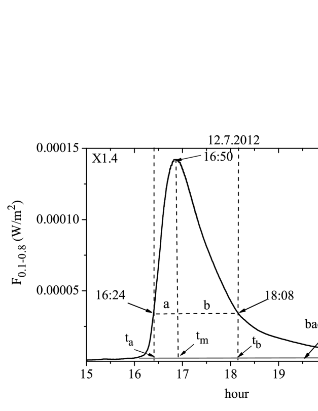
Figure 4: Flare 12.07.2012. The radiation flux in the SXR-range $F_{0.1-0.8}$ according to the observations of GOES-15. The moments of the maximum of flare flux $t_{m}$ and moments of a quarter of the maximum flux value (FWQM) – $t_{a}$ and $t_{b}$ are showed.

To determine XI, we use the value of quarter of the maximum flux (FWQM - full width quarter-maximum). In Figure 3 and Figure 4, the value of a corresponds to the time in minutes that has elapsed from the level of the flux in a quarter of the maximum to the maximum in the rise phase of a flare, the value of b corresponds to the time in minutes from the maximum to the level of the flux in a quarter of the maximum in the decay phase of a flare. We determine the value of the flare index XI as the multiplying the flux in the maximum $F_{0.1-0.8}^{max}$ by the flare duration at the FWQM level that is equal to (a + b).

$$XI=\leavevmode\nobreak\ F_{0.1-0.8}^{max}\cdot(a\leavevmode\nobreak\ +b)\leavevmode\nobreak\ \leavevmode\nobreak\ \leavevmode\nobreak\ \leavevmode\nobreak\ \leavevmode\nobreak\ \leavevmode\nobreak\ \leavevmode\nobreak\ (2)$$

The XI is calculated using the formula (2), the time interval (a+b) is expressed in seconds. So the XI has the dimension $J/m^{2}$ and is approximately equal to the total energy calculated as the integral under the flux curve (after subtraction of the background flux) according to formula (1).

The daily observations of the flux values $F_{0.1-0.8}(t)$ with an observation interval of 2.5 seconds are available on the GOES web-site, available at

https://satdat.ngdc.noaa.gov/sem/goes/data/new_full/ from 2001 to the present in a real time practically.

To determine the $t_{a}$ and $t_{b}$ moments for the flare, according to the GOES data, we find the moment of maximum $t_{m}$. By the magnitude of the flux at the maximum $F_{0.1-0.8}^{max}$, we determine the level FWQM and find the moments $t_{a}$ and $t_{b}$. In Figure 3 $t_{a}=23^{h}20^{m}$, $t_{m}=23^{h}23^{m}$ and $t_{b}=23^{h}34^{m}$. Accordingly, the quantity $(a+b)=t^{b}-t^{a}=14$ minutes (840 seconds).

Thus, from the calculations using formula (2) for the flare of 09.03.2011, the X-ray flare index $XI=1.6E^{-4}\cdot 840=0.1344\leavevmode\nobreak\ J/m^{2}$. That is, the flare of 09.03.2011 has an X-ray index XI1.344E-1. For comparison, the total energy $E_{0.1-0.8}$ that is equal to the area under the flare light curve with allowance for the background level, calculated according to formula (1), $E_{0.1-0.8}=0.107\leavevmode\nobreak\ J/m^{2}$.

For 12.07.2012 flare X-ray XI-index is equal to $XI=1.4E^{-4}\cdot 6480=0.907\leavevmode\nobreak\ J/m^{2}$. Flare index XI9.07E-1, and, moreover, the energy), $E_{0.1-0.8}=0.792\leavevmode\nobreak\ J/m^{2}$. Thus, the value of XI can be successfully used as a preliminary estimate of the total energy $E_{0.1-0.8}$, that in turn is the most important geoeffective characteristic of the flare (Bruevich & Bruevich 2018; Reames 2004).

For a comfortable representation of the characteristics of flares, all information about the flare can be represented by analogy with the X-ray classification: the 09.03.2011 flare (Fig.3) of class X1.6 is characterised by the X-ray flare index XI1.3E-1, the 12.07.2012 flare of class X1.4 is characterised by X-ray flare index XI9.1E-1.

A similar representation of XI value as 1.3E-1 and 7.9E-1 is accepted for use in many computer applications (EXCELL, OrignPRO, etc.).

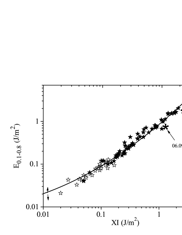
Figure 5: Dependence of the total flare energy in SXR-range on the new X-ray flare index XI for 96 flares of cycle 24. Flares with subsequent proton events are represented by filled asterisks, flares not accompanied by proton events are represented by hollow asterisks. The quadratic regression line and the standard deviation are shown. The largest flares of cycle 24 of 06.09.2017 and 10.09.2017 are marked.

If we mean a flare of classes M and C, then it turns out that the XI values will be two or three orders of magnitude lower than for flares of class X, because for the classes M and C the magnitude of the maximum of flares is 1 – 2 orders of magnitude lower, than for flares of class X, and because weaker flares have shorter duration.

That is, for flares of classes M1 – M9, the X-ray index value may be the order of XI1E-4 – XI1E-2 depending on the flare duration, for the flares of classes C1 – C4 the XI value varies in the range of XI1E-5 – XI1E-3.

Table 1 presents data on 96 major flares in 1998 – 2017 including data on two largest flares of the 24th cycle that occurred in September 2017. We present all the flares of 24th cycle that are more powerful than M5 and some flares of M2 – M5 classes that are characterised by such attendant phenomena such as white light flares. We also added 21 largest flares of the 23rd cycle.

The information on the X-ray class of flares and their duration at the FWQM level for a calculation of the X-ray flare index XI according to formula (2) is obtained from the archival data on the GOES web-site, available at http://www.n3kl.org/sun/noaa_archive/.

Information on the parameters of flares in the $H_{\alpha}$ line is available at //www.ngd.noaa.gov/stp/space-weather/solar-data/.

The energy $E_{0.1-0.8}$ of the flares, and the X-ray flare indices XI are calculated in this paper using equations (1) and (2) and using the data of the GOES web-site, available at

https://satdat.ngdc.noaa.gov/sem/goes/data / new_full /.

The relationship between $E_{0.1-0.8}$ and XI is described by the equation:

$$E_{0.1-0.8}=\leavevmode\nobreak\ 0.0198+0.658\cdot XI+0.106\cdot XI^{2}\leavevmode\nobreak\ \leavevmode\nobreak\ \leavevmode\nobreak\ \leavevmode\nobreak\ \leavevmode\nobreak\ \leavevmode\nobreak\ \leavevmode\nobreak\ (3)$$

Figure 5 demonstrates that for a given set of 24th cycle flares, the X-ray index XI is closely related to the total flare energy in SXR-range $E_{0.1-0.8}$, where the value of XI that is calculated according to formula (2) coincides with $E_{0.1-0.8}$ in dimension ($J/m^{2}$) and practically coincides in magnitude.

Figure 5 also shows the two largest flares that occurred in September 2017. It can be seen that the September 6, 2017 X9.3 flare (the fifth largest since the introduction of the X-ray classification of flares) significantly loses to the 10.09.2017 flare of X8.2 class as by the value of the total energy in SXR-range $E_{0.1-0.8}$, and by the value of the X-ray flare index XI.

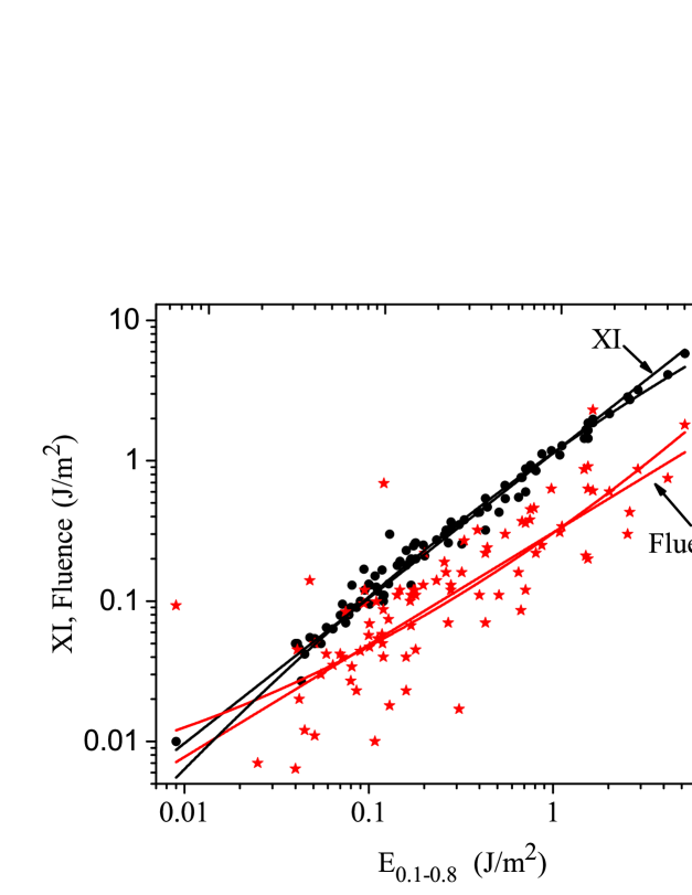
Figure 6: Dependence of the index XI and fluence L on the total flare energy in SXR-range $E_{0.1-0.8}$ for 96 flares of cycles 23 – 24.

So-called fluences (L – the integrated flux from start-max to 1/2 max, in $J/m^{2}$) are often used to estimate the flare energy in the SXR-range (The Catalogue 2008; Preliminary Current Catalogue 2018).

In Figure 6, we can see the dependencies of XI and L versus $E_{0.1-0.8}$. Figure 6 shows both linear regression and quadratic regression dependences. It is seen that the dependence of XI vs $E_{0.1-0.8}$ has a smaller scatter of points than the dependence of L vs $E_{0.1-0.8}$.

As a consequence of this fact – Pearson’s linear correlation coefficients for the XI vs $E_{0.1-0.8}$ dependence R=0.93, and for the L vs $E_{0.1-0.8}$ dependence R=0.75. For quadratic regressions, the sum of the residuals RSS is an order of magnitude less in the XI vs $E_{0.1-0.8}$ dependence than in the L vs $E_{0.1-0.8}$ dependence, which also indicates a closer relationship between the XI-index and the $E_{0.1-0.8}$.

4 XI-index and SXR-flare flux versus Solar Proton Events (SPEs), CME linear speed and Kp-index of geomagnetic activity

Patrolling observations of the Sun in the SXR-range is the basis of the modern classification of solar proton events (SPEs), that are associated with an outstanding flux of high-energy protons. Such proton flux is formed as a result of CME which accompanes large solar flares. It was shown that main role in acceleration of SEPs play interplanetary CMEs that are the main source of interplanetary shock waves (Tylka et al. 2005; Reames 2004). In turn, the coronal CMEs are closely related to large flares originating from the same active area in the Sun (Klein 2005). The most significant results on the study of CMEs in recent years were obtained from observations by the LASCO coronagraph on the SOHO spacecraft (see, for example, the reviews by Gopalswamy (2004), Aschwanden (2005), Gopalswamy et al. (2009), Gopalswamy (2016)). The close relationships between flares and CMEs is confirmed by different facts: a similar evolutionary process and explosive energy release in both cases indicates the similarity of temporal velocity profiles of CMEs and of X-ray flares (Zhang et al. 2001). This fact is confirmed by the the existence of close correlation between the kinetic energy of CME and of X-ray fluence (Gopalswamy et al. 2009).

Thus, X-ray flares, observations of which in real time are the most available for further prediction of geoeffctinve events, are important objects for a comprehensive analysis and classification associated with the energy characteristics of the released energy in solar perturbations of the explosive type.

It should be understood that each flare is individual and not all flare events are manifested in the same way. X-ray observations on the spacecrafts YOHKOH and RHESSI showed the appearance of centres of radiation arising from the flare (Podgorny et al. 2009). In X-ray photos of limbic flares, three radiation sources are observed, two of which are located in the photosphere at the foot of the flare loops. They are associated with electron beams falling along the field lines, accelerated in longitudinal currents in accordance with the prediction of the electrodynamic model. The third source is located above the flare loop in the corona, where, according to the electrodynamic model, the radiation source that appears due to the heating of the plasma after reconnecting in the current layer should be located (Podgorny et al. 2009).

In Bazilevskaya et al. (2015); Belov et al. (2005) it is shown that most of the favorably located (on the Western part of the solar disk) flares of M5 class are more powerful are accompanied by SPEs, and almost all SPEs can be identified with a particular solar flare. The duration and intensity of the injection of protons for the observer in the Ecliptic plane varies from one proton event to another proton event by several orders of magnitude.

The physical basis for the communication of SPEs with SXR-radiation is the fact that the source of heating of the flare plasma can be accelerated electrons, that are accelerated simultaneously with protons. At the same time, there is no theory that connects quantitatively different types of electromagnetic and corpuscular radiation of solar flares (Belov et al. 2005). According to statistical analysis (Li et al. 2013; Sharykin et al. 2012) that was made for several largest proton events of the 23rd and 24th cycle, the time difference from the maximum flux $F_{0.1-0.8}^{max}$ of the flare to the maximum flux of SPE is approximately equal to 35 minutes – 2 hours depending on the path of proton propagation.

In this case, from the graphic data GOES (www.n3kl.org/sun/noaa_archive/) it can be seen that the phase of a sharp increase in the proton flux coincides with the phase of the flare flux decay. Most often, the proton flux ($I_{pr}$) quickly reaches a maximum and for some time (depending on the flare power - up to a couple of days) is kept at a constant level and then slowly decreases.

An important property of the X-ray index XI, as an energy characteristic of the flare, is its obvious connection with proton flares (proton events). Usually, when discussing the relationship between thermal and non-thermal electromagnetic radiation of solar flares, we refer to the similarity of time profiles of the intensity of non-thermal radiation and the derivative on time of SXR-flux (Neupert effect). This similarity corresponds to a single-loop evaporation model, but it is not observed in more than 50% of long-term events and this is due to the long and multiple acceleration of electrons with a variable spectrum in the system of flare loops in different physical conditions (Struminskii 2011).

In the study of the energy release of solar flares, it is necessary to have an idea of the fine structure of the flare region, since many energy release channels depend on the geometric parameters of the magnetic loops along which the energy transfer occurs. The fine structure can affect the density of the accelerated electrons in the beam and their propagation in the plasma.

All these features of various flares manifest themselves in the ambiguity of the relationship between the XI-index, X-ray fluxes in flares and SPEs, as evidenced by the large scatter of values in Figures 7 and 8.

According to the forecast center RUSSIAN HELIOGEOPHYSICAL MONITORING CENTER (http://space-weather.ru/index.php?page=home-en) a geoeffective flare (an event associated with CME) is an event that entails the following change in geomagnetic activity indices:$D_{st}\leqslant$ - 80 and Kp $\geqslant$ 7. With such values of geomagnetic indices, magnetic storms become dangerous both for aviation when flying at an altitude of more than 10,000 m, and ground-based radio communication devices, etc. Also, the onset of GLE is undoubtedly a geoeffective event in which$D_{st}$ can be less than -250-300, and Kp $\geqslant$ 8.

Traditionally, a statistical analysis of flares with subsequent SPE is carried out to identify patterns of interaction between X-ray bursts and geoeffective proton events. Since 1970, SPEs, in which the protons with energy E $\geqslant$ 10 MeV and fluxes $I_{pr}\geqslant 1$ pfu (1 pfu = 1 $cm^{-2}\cdot s^{-1}\cdot sterad^{-1}$) were observed, has been collected in catalogs edited by Yu. I. Logachev, available at www.wdcb.ru/stp/online_data.ru.html. These catalogs are characterized by homogeneous and long time series.

According to flares of 23rd and 24th cycles, only the most common patterns of parent flares and proton fluxes were revealed in Bazilevskaya et al. 2015: when the maximum flare amplitude in the SXR-range was changed from $10^{-6}\leavevmode\nobreak\$to $\leavevmode\nobreak\ 10^{-3}\leavevmode\nobreak\ W\cdot m^{-2}$, the maximum proton flux $I_{pr}$ increased from 0.01 to 100 pfu for protons with E $\geqslant$ 100 MeV. The largest flares that are accompanied by so-called ground-based increases (GLEs) are among the most powerful SPEs and proton fluxes with E $\geqslant$ 100 MeV for such flares are enclosed in the range of 100 – 1000 pfu.

The flares accompanied by GLE are of great interest both for the determination of the mechanisms of acceleration and propagation of charged particles in the Sun and in the interplanetary medium, and for the determination of radiation danger in the near-Earth space. According to the catalogs (The Catalogue 2008; Preliminary Current Catalogue 2018), in 24th cycle only three events with GLE were recorded (17.05.2012, 06.01.2014 and 10.09.2017), while 15 events with GLE were recorded in the cycle 23.

From The Catalogue (2008) and Preliminary Current Catalogue (2018) it also follows that in 2018, when we are already at the minimum between 24th and 25th cycles, the number of events with energy of protons E $\geqslant$ 10 MeV throughout 24th cycle is approximately 30% less than in cycle 23 (60 versus 89, respectively). The comparison of flare parameters from Table 1 is shown in Figure 5. Blackened asterisks indicate flares that accompanied by SPEs with different levels of flux but exceeding the value of 10 pfu for protons with E $\geqslant$ 10 MeV.

Figure 5 demonstrates that flares with subsequent proton event are most likely characterized by X-ray index greater than XI1.0E-1 – XI1.5E-1. This paper examines the relationship between the so-called parent flares and the SPEs that follow them.

Table 1 shows all the flares of 23rd and 24th cycle that are accompanied by SPEs and characterised by $I_{pr}\geqslant 2$ pfu, as well as the most significant flares of 23rd cycle (21 flares with $I_{pr}$ that are characterized by proton fluxes of 100 – 10000 pfu for SPsE with E $\geqslant$ 10 MeV). Some of these flares are accompanied by significant SPEs with E $\geqslant$ 100 MeV.

In Figure 7 and in Figure 8, the dependencies of the X-ray index XI and $F_{0.1-0.8}^{max}$ vs values of proton fluxes with E $\geqslant$ 10 MeV and E $\geqslant$ 100 MeV for 96 parent flares from Table 1 are presented. The quadratic regression lines are marked. Data on proton fluxes in the ranges with E $\geqslant$ 10 MeV and E $\geqslant$ 100 MeV are taken from The Catalogue (2008) and Preliminary Current Catalogue (2018) and also refined directly from the GOES archive data, available at (www.n3kl.org/sun/noaa_archive/).

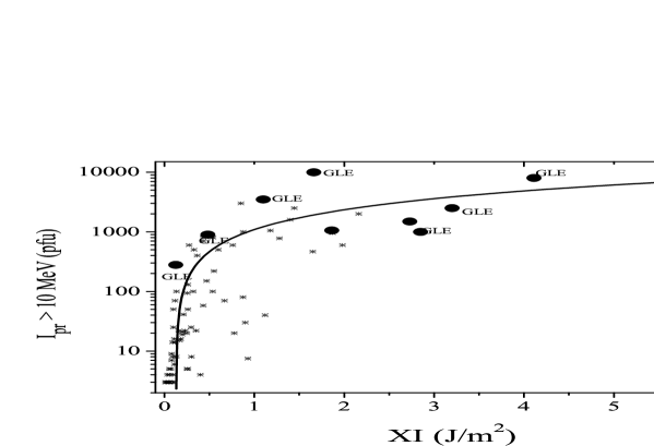
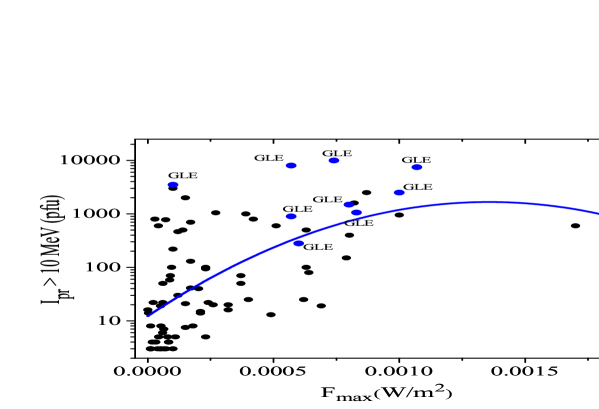
Figure 7: Top: The dependence of the proton flux with energies E $\geqslant$ 10 MeV versus X-ray index XI of the parent flares in cycles 23 and 24; Bottom: The dependence of the proton flux with energies E $\geqslant$ 10 MeV versus $F_{0.1-0.8}^{max}$. The Ground Level Events (GLE) and quadratic regression lines are marked.

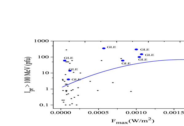
Figure 8: Top: The dependence of the proton flux with energies E $\geqslant$ 100 MeV versus X-ray index XI of the parent flares in cycles 23 and 24; Bottom: The dependence of the proton flux with energies E $\geqslant$ 100 MeV versus $F_{0.1-0.8}^{max}$. The Ground Level Events (GLE) and quadratic regression lines are marked.

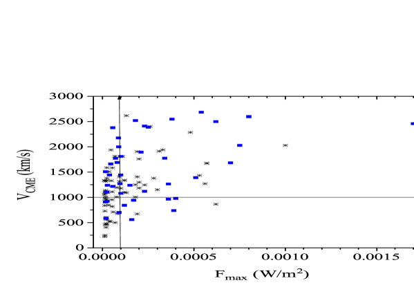
Figure 9: Top: The dependence of CMEs linear speed $V_{CME}$ on the X-ray index XI in cycles 23 and 24; Bottom: the dependence of the CME linear speed $V_{CME}$ versus $F_{0.1-0.8}^{max}$.

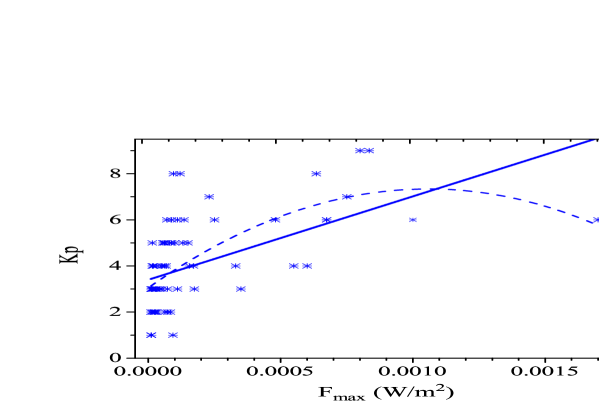
Figure 10: Top: The dependence of the Kp-index of geomagnetic activity on the X-ray index XI in cycles 23 and 24; Bottom: the dependence of the Kp-index of geomagnetic activity versus $F_{0.1-0.8}^{max}$. Linear and quadratic regression lines are marked.

Table 1: Parameters of 96 flares of 23rd and 24th cycles and subsequent Solar Proton Events affecting the earth environment

Date of flare	X-ray class/	X-ray index	Proton flux $I_{pr}$	Proton flux $I_{pr}$
	$H_{\alpha}$-score/	XI	E $\geqslant$ 10 MeV,	E $\geqslant$ 100 MeV
	$H_{\alpha}$-duration, min	($J/m^{2}$)	pfu	pfu
24.08.1998	X1.0/3B/180	0.55	220	4
30.09.1998	M2.8/2N/150	0.43	800	3.5
14.07.2000	X5.7/3B/105/GLE	4.11	8000	400
08.11.2000	M7.4/3F/80/GLE	0.66	10000	300
24.11.2000	X2.3/2B/22	0.255	94	1.2
02.04.2001	X18.4/1B/70	2.85	1000	5.5
09.04.2001	M7.9/1B/70	0.251	5	0.45
10.04.2001	X2.3/3N/176	0.538	100	0.4
15.04.2001	X10.4/3B/130/GLE	1.87	951	100.3
24.09.2001	X2.6/2B/155	1.178	1050	10
01.10.2001	M4.2/2B/160	0.76	600	0.2
04.11.2001	X1.0/3B/450/GLE	0.85	3000	50
22.11.2001	X1.0/2B/160/GLE	1.1	3500	4
26.12.2001	M7.1/1B/230/GLE	1.28	779	50
21.04.2002	X1.5/1F/125	2.16	2000	20
26.10.2003	X1.2/1N/170	1.65	466	1.0
28.10.2003	X10.7/4B/280/GLE	5.8	7500	150
29.10.2003	X10.0/2B/150/GLE	3.2	2500	100
02.11.2003	X8.3/2B/170	1.86	1060	40
03.11.2003	X3.9/2F/50	0.875	1000	3
04.11.2003	X17/3B/80	1.98	600	1.1
28.01.2011	Рњ1.3/1F/30	0.01	3	-
15.02.2011	X2.2/2F/25	0.02	3	-
07.03.2011	M3.7/1F/90	0.259	50	0.15
07.06.2011	M2.5/2N/100	0.1	50	4
14.06.2011	M1.3/SF/40	0.30	8	-
04.08.2011	M9.3/2B/84	0.118	70	1.5
08.08.2011	M3.5/1B/55	0.054	4	-
09.08.2011	X6.9/2B/72	0.296	25	2.5
06.09.2011	X2.1/2B/55	0.167	15	0.1
07.09.2011	X1.8/3B/74	0.13	8	0.3

Table 2: Continuation of Table 1

Date of flare	X-ray class/	X-ray index	Proton flux $I_{pr}$	Proton flux $I_{pr}$
	$H_{\alpha}$-score/	XI	E $\geqslant$ 10 MeV,	E $\geqslant$ 100 MeV
	$H_{\alpha}$-duration, min	($J/m^{2}$)	pfu	pfu
22.10.2011	M1.3/1N/130	0.26	5	-
03.11.2011	X1.9/2B/82	0.4	4	-
25.12.2011	M4.0/1N/60	0.054	3.0	-
23.01.2012	M8.7/2B/335	1.443	2500	2.2
27.01.2012	X1.7/2F/96	0.428	700	11
05.03.2012	X1.0/2B/105	0.1	3	-
07.03.2012	X5.4/3B/220	1.40	1600	60
09.03.2012	M6.3/SF/160	0.329	500	8
13.03.2012	M7.9/1B/185	0.469	150	2
17.05.2012	M5.1/1F/93/GLE	0.126	280	20
14.06.2012	M2.1/2B/150	0.12	14	-
06.07.2012	M6.2/1B/40	0.1	25	-
08.07.2012	M6.9/1N/23	0.2	19	-
12.07.2012	X1.4/2B/250	0.873	80	0.25
17.07.2012	M1.7/1F/250	0.26	130	-
19.07.2012	M7.7/SF/155	0.667	70	0.8
08.11.2012	M1.7/1F/40	0.05	3	-
14.11.2012	M1.1/1F/10	0.08	9	-
15.03.2013	M1.1/1N/180	0.18	16	-
11.04.2013	M6.5/3B/125	0.133	100	2
13.05.2013	X1.7/1N/39	0.21	41	-
15.05.2013	X1.2/2N/66	0.248	20	0.1
22.05.2013	M5.0/3N/180	0.273	600	3
21.06.2013	M2.9/1F/87	0.11	6	-
23.06.2013	M2.9/1N/12	0.09	14	-
28.10.2013	X1.0/2N/50	0.07	5	-
29.10.2013	X2.3/1N/20	0.055	5	-
01.11.2013	M6.3/1B/70	0.06	3	-
06.11.2013	M1.8/1F/40	0.08	7	-
19.11.2013	X1.0/SF/80	0.035	4	-

Table 3: Continuation of Table 1

Date of flare	X-ray class/	X-ray index	Proton flux $I_{pr}$	Proton flux $I_{pr}$
	$H_{\alpha}$-score/	XI	E $\geqslant$ 10 MeV,	E $\geqslant$ 100 MeV
	$H_{\alpha}$-duration, min	($J/m^{2}$)	pfu	pfu
07.01.2014	X1.2/2N/76/GLE	0.481	900	4
20.02.2014	M3.0/SN/60	0.16	22	0.8
25.02.2014	X4.9/2B/90	0.777	20	0.8
29.03.2014	X1.0/2B/40	0.0792	3	0.5
18.04.2014	M7.3/1N/50	0.43	58	0.7
10.09.2014	X1.6/2B/240	0.899	30	0.9
13.12.2014	M1.5/1F/15	0.05	3	-
20.12.2014	X1.8/3B/90	0.038	3	-
15.03.2015	M1.2/1F/40	0.09	8	-
18.06.2015	M1.2/1N/80	0.11	16	-
21.06.2015	M2.0/1N/120	0.32	100	0.2
21.06.2015	M6.5/2B/170	0.6	500	0.1
25.06.2015	M7.9/3B/63	0.35	22	-
20.09.2015	M2.1/2N/120	0.05	3	-
09.11.2015	M3.9/2N/65	0.095	4	-
28.12.2015	M1.8/1F/120	0.02	3	-
01.01.2016	M2.3/1N/105	0.2	21	-
14.07.2017	M2.4/1N/180	0.23	22	-
04.09.2017	M7.0/2N/90	0.54	800	0.8
06.09.2017	X9.3/2B/40	1.12	40	0.7
07.09.2017	X1.4/2B/120	0.366	400	0.8
10.09.2017	X8.2/3B/120/GLE	2.73	1490	60

Figure 7 and Figure 8 show that the spread in values of proton fluxes from quadratic regression lines (that are marked in the figures) is sufficiently large, which confirms the complexity and variety of flares and associated SPEs. It can also be seen that in cases when SPEs of different power are analysed depending on the XI- index as compared to the dependence on the $F_{0.1-0.8}^{max}$, the spread of values in the first case (XI- index) is less. Note that when we use the linear (not log) scales in Figures 7a,8a and 7b,8b and analise the dependencies with linear regressions, then for dependencies in Figures 7a,8a the Pearson’s correlation coefficient will be approximately equal to 0.6-0.7, and for Figures 7b,8b – approximately 0.3-0.4. We can make an assessment (according to Figure 7a) that in case when XI$>$ 0.5 and Ipr$>$ 200 are simultaneously satisfied, then the probability of GLE is approximately 0.5.

In Figures 9a, 9b the possibility of the simple prediction of the geoeffective event characterised by high geomagnetic activity $D_{ST}\leqslant-80$ caused by explosive events in the Sun demonstrate. As noted above, the similarity of CME speed $V_{SME}$ profiles to that of flare soft X-ray emission peculiar properties takes place (Zhang et al. 2001).

Figure 9a shows the relationship between the $V_{SME}$ and the XI-index for the flares with CMEs, taking into account the dependence on the value of the $D_{ST}$ index. Large circles correspond to the case with geomagnetic index $D_{ST}\leqslant-80$. In Figure 9b – the relationship between the $V_{SME}$ and the $F_{0.1-0.8}^{max}$ for the flares with CMEs, taking into account the dependence on the value of the $D_{ST}$ index. Large squares correspond to the case with geomagnetic index $D_{ST}\leqslant-80$.

In Figure 9a it was shown a region characterised by $V_{SME}\geqslant 1000$ together with XI $\geqslant 0.25$. In this region, there are 46 points, among which 35 points are geoeffective with $D_{ST}\leqslant-80$ (large circles). Thus, the probability of a geoeffective event with $D_{ST}\leqslant-80$ is 35/46=0.76.

In Figure 9b, it was shown a region characterized by $V_{SME}\geqslant 1000$ together with $F_{0.1-0.8}^{max}\geqslant 0.0001$ (Flares of class more or equal to X1). The $F_{0.1-0.8}^{max}$ values on Figure 9b were chosen so that the number of points in the selected area coincided with the number points in the selected area in Figure 9a and was also equal to 46. The probability of a geoeffective event with $D_{ST}\leqslant-80$ in this case is 26/46=0.56. The advantage of the XI-index is obvious in this case.

Figure 10 shows the dependencies of the global planetary Kp-index of geomagnetic activity on the XI-index of flares, which, together with the associated CMEs, are the sources of magnetic storms. The Kp-index ranges from 0 to 9, where a value of 0 means no geomagnetic activity, and a value of 9 means an extreme geomagnetic storm. For the events of cycles 23 and 24 from our sample, there were no magnetic storms with Kp = 9. The flares (or their XI-indexes) on the Figures 10a,b are the same as those presented in Table 1. Note that not all flares from Table 1 were accompanied by geomagnetic activity (SPEs, magnetic storms), since events that subsequently become geoeffective should come from active regions located in the western part of solar disk.

It can be seen that the interconnection between the variables in the case of Figure 10a is closer than in the case of Figure 10b (the Pearson’s correlation coefficient R=0.75 in Figure 10a vs. R=0.45 in Figure 10b).

Figure 11: The dependency of a from b for 96 flares of cycles 23 and 24 studied in this work. The quadratic regression line and the standard deviation are shown.

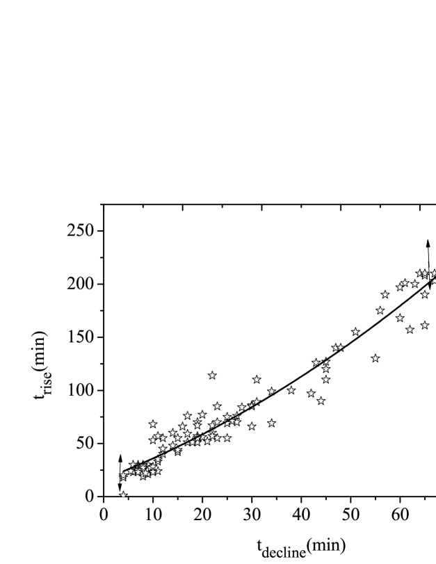
Figure 12: The dependency of $t_{rise}$ from $t_{desay}$ for 96 flares of cycles 23 and 24 studied in this work. The quadratic regression line and the standard deviation are shown.

Note that the calculation of the X-ray index XI for a particular flare is very simple: we have to determine from the GOES archive data the level of FWQM that is equal to one quarter of the flux at the maximum, then to determine the moments $t_{a}$ and $t_{b}$ and to use formula (2).

Observations of GOES are presented with an interval of 2.5 seconds, which entails an error in determining of the X-ray index XI only in the third-fourth significant digit (less than 0.1%). A calculation the value of energy $E_{0.1-0.8}$ (as the flare characteristics that is compared to XI) requires much more efforts: to integrate the flare light curve, you need to convert the archived GOES data, linking them to the real time-scales and correctly select the background level. Finally, the error in the definition of $E_{0.1-0.8}$ can already reach several percent. In particular, due to the fact that the background level before and after the flare may vary, and this introduces uncertainty in determining the flare end time.

5 Relationship between rising and declining phases of solar flares

To calculate the index XI, it is important to determine the times $t_{a}$ and $t_{b}$ (intervals a and b) most precisely. For GOES data, this is not difficult, except when flares go on overlapping one another before they reach the level of the background flux during the phase of decline. In this case, the following comparative analysis of the data on the relationship between the phase of rise and phase of decline of flares can help.

In this paper, we investigated the relationship between the parameters $a$ and $b$ for a sample of 96 significantly more powerful flares of classes M2 – X9 from the Table 1.

The relationship between the parameters $a$ and $b$, expressed in seconds, is shown in Figure 9. The relationship between the values of $a$ and $b$ is described by the quadratic regression equation:

$$b=356+1.32\cdot a+0.0018\cdot a^{2}\leavevmode\nobreak\ \leavevmode\nobreak\ \leavevmode\nobreak\ \leavevmode\nobreak\ (4)$$

Thus, taking into account the dependence (4), it is possible to estimate the time $t_{b}$ in complex cases, when flares follow one after another and one flare is applied to subsequent flare. For some flares, there is a discrepancy in the determination of the time of beginning and ending of the flare in $H_{\alpha}$ in different observatories. Sometimes observers simply indicate that the flare lasts more than a certain time. This introduces uncertainty in the calculation of the FI flare index.

To correctly determine the duration of $H_{\alpha}$ flares for 96 flares from Table 1, the connection between the duration from the beginning of the flare to its maximum ($t_{rise}$) and the duration from the flare maximum to its end ($t_{decay}$) is studied. $t_{rise}$ and $t_{decay}$ correspond to a full interval of time in the rise phase and in the decline phase of the flare, taking into account the excess of radiation from flares above the level of background in $H_{\alpha}$.

In Figure 12, the relationship between $t_{rise}$ and $t_{decay}$ is described by a quadratic regression equation with a relatively small second-order term:

$$t_{decay}=17.68+2.006\cdot t_{rise}+0.0145\cdot t_{rise}^{2}\leavevmode\nobreak\ \leavevmode\nobreak\ \leavevmode\nobreak\ \leavevmode\nobreak\ (5)$$

Using dependencies (4) and (5), you can determine the values of the time intervals $b$ and $t_{decay}$ that are necessary to calculate the X-ray index XI and the optical index FI in cases where it is impossible to determine the parameters $b$ and $t_{decay}$ directly from observations.

6 Conclusion

The method of additional flare classification proposed in this paper based on determining the X-ray flare index XI by analogy with the optical flare index FI has the following advantages:

1. The X-ray index XI is easily calculated according to formula (2). Data on the values of $a$, $b$, $F_{0.1-0.8}^{max}$, $F_{background}$ are available on the GOES web-site (from 1978 to the present). Accordingly, for each flare, the X-ray index XI can be calculated, starting from 1978.

2. X-ray index XI is an analog of the total energy of flare in SXR-range $E_{0.1-0.8}$ that can be calculated according to formula (1). The relationship between XI and $E_{0.1-0.8}$ is described by (3), resulting if you know the index XI, you can rapidly evaluate the flare parameter $E_{0.1-0.8}$.

3. By the value of the index XI, as well as by the value $E_{0.1-0.8}$, it is possible to determine flares with subsequent SPEs (under the condition of localization of the flare region in the western part of the Sun’s disk suitable for propagation of protons towards the Earth).

4. X-ray index XI, as well as $E_{0.1-0.8}$, is the most important geoeffective parameter of the flare. The combined use of XI and of the most important parameters of flares, as well as associated CMEs, it is possible to predict the probability of occurrence of geoeffective events of various scales, that characterised by the geomagnetic indices Dst and Kp.

References

Altyntsev A. T., Banin V. G., Kuklin G. V., Tomozov V. V. 1982, Solar Flares, Moscow.: Nauka

Aschwanden M. J. 2005, Physics of the Solar Corona. Springer, Berlin.

Bazilevskaya G. A., Logachev Yu. I., Vashenyuk E.V. et al. 2015, Bulletin of the Russian Academy of Sciences: Physics, 79, p. 627

Belov A., Garcia N., Kurt V. et al. 2005, Solar Physics, 229, p. 135

Bogod V. M. 2006, Bulletin of the Russian Academy of Sciences: Physics, 70, p. 491

Bogod V. M. 2011, Astrophysical Bulletin, 66, p. 190

Bowen T. A., Testa P., Reeves K. K. 2013a, LWS/SDO Science Workshop, (SOC), Cambridge, USA

Bowen T. A., Testa P., Reeves K. K. 2013b, Astrophysical Journal, 770, p. 126

Bruevich E. A., Yakunina G. V. 2017, Astrophysics, 60, p. 387

Bruevich E. A., Bruevich V. V. 2018, Astrophysics, 61, p. 241

Gopalswamy N. A. 2004, Astrophys. Space Sci. Libr., 317. p. 201

Gopalswamy N., Yashiro S., Michalek G., Stenborg G., Vourlidas A., Freeland S., Howard R. 2009, Earth, Moon, and Planets, 104, p. 295

Gopalswamy N. 2016, Geoscience Letters, 3, article id.8, 18 pp

Kleczek J. 1952, Publ. Czech Centr. Astron. Inst., 22, p. 1

Klein K.-L., Krucker S., Trottet G., Hoang S. 2005, Astron. Astrophys., 431, p. 1047

Li C., Firoz K. A., Sun L. P., Miroshnichenko L. I. 2013, ApJ, 770, article id. 34, 12 pp

Ozgus A., Atac T., Rybak J. 2003, Solar Physics, 214, p. 375

Preliminary Current Catalogue of Solar Flare Events. 2018,

//www.wdcb.ru/stp/data/Solar_Flare_Events/Fl_XXIV.pdf

Podgorny I. M., Vashenyuk E. V., Podgorny A. I. 2009, Geomagnetism and Aeronomy, 49, p. 1115

Reames D. V. 2004, Adv. Space Res., 34(2), p. 381

Sharykin I. N., Struminsky A. B., Zimovetz I. V. 2012, Astronomy Letters, 38, p. 672

Somov B. V., Syrovatskii S. I. 1976, Soviet Physics Uspekhi, 19, p. 813

Struminskii A.B. 2011, Bulletin of the Russian Academy of Sciences: Physics, 75, p. 751

The Catalogue of Solar Flare Events. 2008, //ww.wdcb.ru/stp/data/Solar

_Flare_Events/Fl_XXIII.pdf.

Tylka A., Cohen W. F., Dietrich M. A. et al. 2005, ApJ, 625, p. 474

Zhang J., Dere K. P., Howard R. A., Kundu M. R., White S. M. 2001, Astrophys. J., 559, p. 452