Trusted Neural Networks for
Safety-Constrained Autonomous Control

Abstract

We propose Trusted Neural Network (TNN) models, which are deep neural network models that satisfy safety constraints critical to the application domain. We investigate different mechanisms for incorporating rule-based knowledge in the form of first-order logic constraints into a TNN model, where rules that encode safety are accompanied by weights indicating their relative importance. This framework allows the TNN model to learn from knowledge available in form of data as well as logical rules. We propose multiple approaches for solving this problem: (a) a multi-headed model structure that allows trade-off between satisfying logical constraints and fitting training data in a unified training framework, and (b) creating a constrained optimization problem and solving it in dual formulation by posing a new constrained loss function and using a proximal gradient descent algorithm. We demonstrate the efficacy of our TNN framework through experiments using the open-source TORCS [27] 3D simulator for self-driving cars. Experiments using our first approach of a multi-headed TNN model, on a dataset generated by a customized version of TORCS, show that (1) adding safety constraints to a neural network model results in increased performance and safety, and (2) the improvement increases with increasing importance of the safety constraints. Experiments were also performed using the second approach of proximal algorithm for constrained optimization — they demonstrate how the proposed method ensures that (1) the overall TNN model satisfies the constraints even when the training data violates some of the constraints, and (2) the proximal gradient descent algorithm on the constrained objective converges faster than the unconstrained version.

1 Introduction

Deep learning algorithms generally assume a parametric (typically non-linear) model and fit the training data to the model to minimize the loss between true output and model’s output. Sometimes, we also impose regularization constraints on parameters to avoid overfitting. However, in some applications it is important to impose additional constraints on the model output, such as constraints enforcing safety properties inherent in the domain. For example, when driving along a straight road, the autonomous controller for a self-driving car should not cross a double-yellow line. Another example could be a medical transcription tool that is faced with ambiguity when translating text. Domain knowledge regarding safe drug prescription boundaries can mitigate erroneous transcriptions indicating an unhealthy high dosage for a medication. In this paper, we investigate methods to add constraints on the output of a deep neural network model as an additional objective that has to be satisfied during training, even when the training data might violate the constraints on some occasions. We call the resulting models Trusted Neural Networks (TNN), as they are deep neural network models that satisfy safety constraints critical to the application domain. In this paper, we propose two approaches for designing TNN models:

(1) One approach is using a multi-headed model architecture [2], where one “head” (i.e., tower of neural network layers) fits the labeled data while another head fits the logic constraints, and both heads have a set of common layers for parameter sharing. The whole model is then trained jointly, effectively having a combined loss function with a trade-off parameter that controls the desired importance of the logic constraints. We run experiments using the open-source TORCS [27] 3D simulator for self-driving cars to show that (a) adding informative constraints to a baseline model allows it to predict safer results, and (b) increasing the importance given to the rules gives improved results.

(2) Second approach considers the constraints in the objective function using a dual formulation, i.e., optimizing a new loss function that is a weighted sum of the original loss function and a function representing the constraints. We use proximal gradient descent to optimize this new loss function. We run experiments using the simulator, and demonstrate that our constrained learning approach manages to (a) impose important constraints on the model, and (b) guide the model in reaching the optimal point faster.

In this paper we individually evaluate these two methods. We don’t compare them to each other, since the two methods would in the limit generate models with similar performance (e.g., MSE) when the constraints are known and enforced strictly. In cases where the logical constraints are not known but needs to be learned from data, we use the multi-headed model formulation where the logic head learns an approximation of the constraints from data. When we know the form of the constraints for certain, it may be better to use the constrained learning formulation, since it can in general converge to the optimum value faster during training.

2 Problem Formulation

Deep learning methods for training neural networks fit a function $f$ between input ($i$) and output ($o^{\prime}$) and learn the parameters (weights) $w$ so that the model’s output ($o^{\prime}$) is close to true output ($o$). The learning part can be posed as an optimization problem, where $\ell$ is a loss function:

$$\min_{w}\ell(o,o^{\prime}),\quad\text{s.t. }o^{\prime}=f(w,i).$$

Occasionally, we add a further constraint on weights to avoid overfitting, giving us a regularized loss function:

$$\min_{w}\ell(o,o^{\prime})+\ell^{\prime}(w),\quad\text{s.t. }o^{\prime}=f(w,i)$$

where $\ell^{\prime}$ is a regularization function. To satisfy safety constraints, we consider imposing additional constraints directly on model’s output, giving a constrained loss function:

$$\min_{w}\ell(o,o^{\prime}),\quad\text{s.t. }o^{\prime}=f(w,i)\ \mbox{and}\ g(o^{\prime})\leq 0$$ (1)

where $g$ is a function, possibly in first-order logic, specifying the safety constraints. In this paper, we study two possible ways of training trusted neural network (TNN) models by solving the optimization problem given in Equation 1.

3 Trusted Neural Networks

The first approach for training TNN models uses a multi-headed model architecture to learn from two different sources of knowledge: data-based and rule-based.

3.1 Multi-headed models

In the multi-headed architecture, each of the model’s heads has its own objective function and is adapted to the problem they have to solve — they share a neural network (set of layers), called the shared net. One example of a multi-headed network is given in Figure 2; let the parameters of the head 1, the head 2 and the shared network be $p_{1}$, $p_{2}$ and $p_{s}$ respectively. Here, head 1 has the objective function $O_{1}(p_{1},p_{s})$ and head 2 has the objective function $O_{2}(p_{2},p_{s})$. The model is then jointly trained with the combined loss function, $O_{1}(p_{1},p_{s})+\lambda O_{2}(p_{2},p_{s})$ where $\lambda\in\mathbb{R^{+}}$ is a parameter fixing a trade-off — it determines the importance given to the rule-based knowledge source.

Note that if we need the constraints to be strictly enforced, we can set a very high value of $\lambda$. Having soft constraint satisfaction using the Lagrangian formulation allows us to enforce the constraints with different levels of strictness, which can be enforced based on the domain requirements.

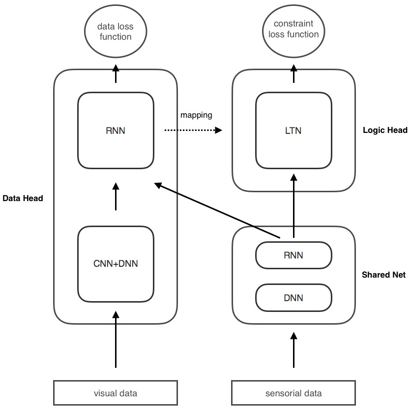
Figure 1: The multi-headed TNN model.

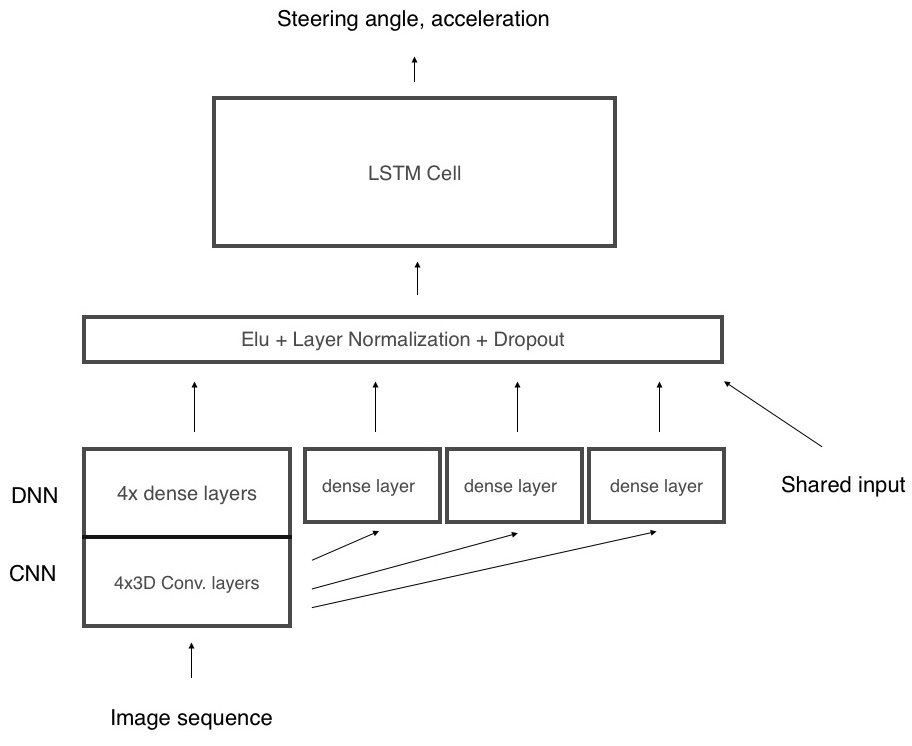
Figure 2: The data head.

3.1.1 Network on logical constraints

To fit logic rules in the logic head, we chose to use and extend Logic Tensor Networks [24], i.e., LTN. In LTNs, we define a language using first-order logic $\mathcal{L}(\mathcal{C},\mathcal{F},\mathcal{P})$, where $\mathcal{C}$ is the set of constants (data points), $\mathcal{F}$ the function symbols, and $\mathcal{P}$ the predicate symbols. The goal of LTNs is to typically learn the function $g$ in Equation 1, from both data and rule-based knowledge (written as first-order logic rules). To do this, a grounding is defined on the language $\mathcal{L}$, mapping logical propositions to their truth values in $[0,1]$. Constants are mapped to numerical vectors; the symbols we want to learn are mapped to functions whose parameters are learned using gradient descent, to maximize an objective function that is the conjunction of clauses defined over the data points. In the TNN model, we jointly train a network (the data head) on the data and a LTN (the logic head) on the rules, using a combined loss function.

The functional operators in the LTN are mapped to small deep regression neural networks. The LTN has to effectively encode logical functions in a neural network, for which it uses real logic [24]. Real logic is defined as follows. Let $\mathcal{G}$ be the grounding used in the real logic framework, and $f$ a real unary functional operator $f:\mathcal{C}\rightarrow\mathbb{R}^{p}$ that will be mapped to the function $\mathcal{G}(f):\mathbb{R}^{d}\rightarrow\mathbb{R}^{p}.$ The definition of the grounding $\mathcal{G}$ is extended to a new class of literals using the functional operator $f$; mainly, for a data point $x\in\mathcal{C}$ and $c\in f(\mathcal{C}),$ $f(x)=c$, $f(x)\geq c$ and $f(x)\leq c,$ are:

$$\mathcal{G}(f(x)=c)\in[0,1],\quad\mathcal{G}(f(x)=c)=1\iff f(x)=c,$$

$$\mathcal{G}(f(x)\leq c)\in[0,1],\quad\mathcal{G}(f(x)\leq c)=1\iff f(x)\leq c,$$

$$\mathcal{G}(f(x)\geq c)\in[0,1],\quad\mathcal{G}(f(x)\geq c)=1\iff f(x)\geq c.$$

Possibilities include using functions such as :

$$\mathcal{G}(f(x)=c)=1-exp(||f(x)-c||^{2})$$ (2)

and if $f(\mathcal{C})$ is bounded with a diameter $\delta(\mathcal{C})$

$$\mathcal{G}(f(x)=c)=1-\left|\left|\frac{f(x)-c}{\delta(\mathcal{C})}\right|\right|^{2},\ \mbox{or}$$ (3)

$$\mathcal{G}(f(x)=c)=1-\left|\frac{f(x)-c}{\delta(\mathcal{C})}\right|.$$ (4)

The function in Equation (2) provides very low gradients outside of the truth region, while Equation (4) is non-differentiable on 0; we decided to use Equation (3), standard in the field of regression, as the functional operators considered have defined bounds. Adapting to the other literals :

$$\mathcal{G}(f(x)\leq c)=1-\left|\left|\max\left(\frac{f(x)-c}{\delta(\mathcal{C})},0\right)\right|\right|^{2},\quad\mathcal{G}(f(x)\geq c)=1-\left|\left|\min\left(\frac{f(x)-c}{\delta(\mathcal{C})},0\right)\right|\right|^{2}.$$

To implement bounded regression neural networks, we use a $tanh$ activation function on the output layer and rescale the output with the desired mean and range vectors. Assume $f(\mathcal{C})\subset[a_{0};b_{0}]\times[a_{1};b_{1}]\times...\times[a_{p};b_{p}]$ with $a_{0},...,a_{p},b_{0},...,b_{p}\in\mathbb{R}.$ Define $m=\frac{1}{2}(a_{0}+b_{0},a_{1}+b_{1},...,a_{p}+b_{p})$ and $r=\frac{1}{2}(b_{0}-a_{0},b_{1}-a_{1},...,b_{p}-a_{p})$. Then the output of the neural network is $m+r\odot tanh(y)$, where $y$ is the output of the last layer of the neural network under consideration.

The model learns from the rules provided that any precondition of the rule is present in the dataset. Otherwise, the rule is considered as satisfied by the model.

3.2 Constrained Neural Network Learning

In our second approach, we solve the problem in Equation 1 by projecting the optimization problem in dual space as:

$$\min_{w}\ell(o,o^{\prime})+\lambda g(o^{\prime})\quad\text{s.t. }o^{\prime}=f(w,i),\quad\quad\lambda\geq 0$$ (5)

Using grid search we can explore over possible values of hyperparameter $\lambda$ and find the best value. Greater values of $\lambda$ give more significance to the constraint function. We solve the above optimization problem (5) using stochastic proximal gradient descent [21, 9]. Proximal gradient descent updates the parameters in two steps:

$$w_{t+1/2} =w_{t}-\eta_{t}\partial\ell(w_{t})$$

$$w_{t+1} =\arg\min_{w}\left(\frac{1}{2}\left\lVert w-w_{t+1/2}\right\rVert^{2}+\eta_{t}\lambda g(w)\right).$$

where in step 1 parameters move along in the direction of gradient of $\ell$ and in step 2 we do proximal mapping of $g$.

Notice that first step is regular gradient descent and can be implemented using backpropagation. The second step is the proximal mapping and for simple $g$ functions, we can have closed form proximal mappings. In other cases, we can use the backpropagation algorithm to find an approximation.

4 Related Work

Machine learning (ML) has a rich history of learning under constraints [8, 19] — different types of learning algorithms have been proposed for handling various kinds of constraints. Propositional constraints on size [3], monotonicity [14], time and ordering [15], etc. have been incorporated into learning algorithms using constrained optimization [4] or constraint programming [22], while first order logic constraints have also been introduced into ML models [18, 23].

Hu et al. [13] incorporated logic rules into a DNN or RNN using a teacher/student network — they iteratively train a student network on the data and project the student network onto the set of given rules to get the teacher network. Towell et al. [26] have also encoded propositional rules into neural networks. Our approaches, based on multi-headed NNs or constrained loss functions, are more flexible, allowing a fine-tuned trade-off between rule constraints and data knowledge, and enables constrained-guided data-efficient learning in a novel way. Ghosh et al. [11] proposed a methodology to ensure that probabilistic models learned from data can also satisfy safety constraints expressed as first-order logic rules.

Proximal gradient descent has been used to optimize convex functions in ML frameworks other than neural networks [5, 10, 7, 17, 25]. Proximal gradient descent has been used in neural network frameworks for regularization [9]. Constrained optimization in neural networks has also been studied [24], where Real Logic (first order logic constraints which have truth value in range $[0,1]$ and real number semantics) have been integrated with the neural networks framework.

5 Experimental Evaluation

5.1 Multi-headed TNN model

We demonstrate the usefulness of the multi-headed TNN model using experiments with an autonomous car controller. We implemented our neural network models in Tensorflow [1].

5.1.1 Car controller

Car control is an example ML problem where logic constraints (e.g., regarding safety) could be used in addition to training data from sensors to produce better and safer models. We developed a customized version of the open-source TORCS [27] 3D car simulator for self-driving cars, which is used for car racing competitions. It gives access to a variety of numeric sensors to help control the car — distance to the edge of the track or to the closest opponent in a set of directions, speed, distance and angle to the center of the track. The problem is to control a set of 5 variables: acceleration, brake, clutch, gear, and steering angle. In our customized version of TORCS, the ML model has also access to the front camera of the car. We assume there are no other cars on the road. The driving state we consider is a vector $(I,S,A)$ where $I$ is the front camera image, $S$ is the numerical vector of the sensors, and $A$ is the action vector.

5.1.2 Dataset

For generating the datasets, we considered a simple car controller with a fixed objective speed and position on the track. The behavior of the vehicle in the simulator is recorded on 10 different tracks included in TORCS, at a framerate of 17 frames per second. The resulting dataset includes image from the front camera, sensorial time trace, and output data. We create two datasets for experimentation. Dataset A is generated based on a deterministic driving pattern, while in Dataset B we introduce some randomness in parameters like track objective. Dataset B has a more diverse driving behavior than dataset A

5.1.3 Multi-headed model

The full multi-headed TNN model, depicted Fig. 2, is jointly trained with a combined loss function:

$$totalLoss=dataLoss+\lambda_{loss}.logicLoss$$

where $dataLoss$ is the loss function relative to the data head, and $logicLoss$ is the one relative to the logic head.

5.1.4 Shared net

The shared net is a Long short-term memory (LSTM) cell [12] built on top of a small deep neural network with two ReLu-activated layers [20]. The input of the shared net is the time trace of the sensorial data, and its output is connected to both data and logic heads.

5.1.5 Data head

The data head is the baseline for our problem. In the Udacity challenge #2 [6], where competitors had to predict steering angle from a sequence of image, the winner used a sequential model (RNN) based on a customized LSTM cell on top of a deep convolutional neural net (CNN) [16] — we considered that as our baseline model.

The goal of the data head is: given a sequence of images and sensorial vectors, predict the steering angle sequence. We add the acceleration to the predicted variables to force the model to learn more precisely the momentum of the car. The data head, as depicted in Fig. 2, is an LSTM cell whose input is the concatenation of the output of two nets — one deep convolutional neural net made of 4 ReLu-activated convolutional layers and 4 ReLu-activated dense layers, and the output of the shared net. The data head uses the mean square error (MSE) loss function.

5.1.6 Logic head

The logic head uses the output of the data head to map the data points: a data point is mapped to the vector $(S,dataHeadOutput)$, where S is the sensorial time trace. Fig. 4 explains how we design a rule for our experiment. Let $a,b,c$ be the oriented angles depicted in Fig. 4. We have:

$$\begin{cases}a=-S[^{\prime}angleToTrack^{\prime}],\\ b=S[^{\prime}steeringAngle^{\prime}],\\ c=a+b=S[^{\prime}steeringAngle^{\prime}]-S[^{\prime}angleToTrack^{\prime}]\end{cases}$$

Intuitively, if the car is close to the right edge of the road, we want $c>0$ ; if the car is on the left edge of the road, we want $c<0$. This gives the following set of two rules :

$$\begin{cases}ifS[^{\prime}trackPosition^{\prime}]<-0.75,\quad S[^{\prime}steeringAngle^{\prime}]-S[^{\prime}angleToTrack^{\prime}]>0\\ ifS[^{\prime}trackPosition^{\prime}]>+0.75,\quad S[^{\prime}steeringAngle^{\prime}]-S[^{\prime}angleToTrack^{\prime}]<0\end{cases}$$

To implement these rules, we define a functional operator $steeringAngle:\mathcal{C}\rightarrow[-1,1]$ that is mapped to a small bounded deep neural network. The rules are encoded using the real logic framework and define, for a given batch of data points and for each rule, the truth values $ruleClauseLeft$ and $ruleClauseRight$. We add the clauses stating that the output of $steeringAngle$ for each element of the batch has to be the ground truth value, which defines a truth value $steeringClause$. These clauses are aggregated using a weighted sum — the weight for $steeringClause$ is fixed to 1, and the weight for each rule is a parameter to define using cross validation: $w_{rule}.$ As a result, we have:

$$logicLoss=1-\frac{1}{1+2w_{rule}}(steeringClause+w_{rule}(ruleClauseLeft+ruleClauseRight)).$$

5.1.7 Evaluation metrics

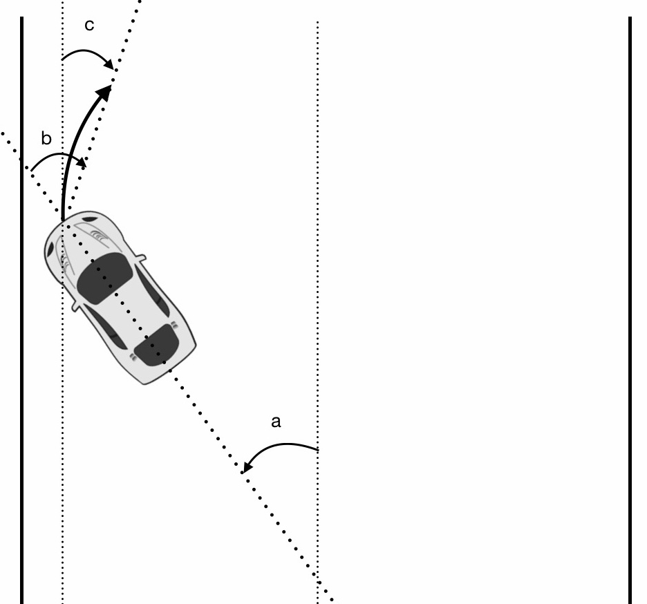
Figure 3: Geometric variables in the TORCS setup.

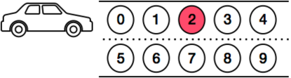
Figure 4: State map with obstacle at state 2.

We evaluate the model against the baseline (data head without the logic head) on two different metrics:

(1) The first metric is the mean square error against the ground truth for steering angle prediction. It evaluates how well knowledge from data is integrated into the model.

(2) The second metric uses the logic head rules. The goal is to evaluate how well the rules have been learned by the model. For a sequence of driving states $((I_{1},S_{1},A_{1}),...,(I_{L},S_{L},A_{L})),$ where $A_{1},..,A_{L}$ is the prediction of the model, let $c_{i}=S_{i}[^{\prime}steeringAngle^{\prime}]-S_{i}[^{\prime}angleToTrack^{\prime}]$ for each state. Note that $c_{i}$ should be negative when $S_{i}[^{\prime}trackPosition^{\prime}]\geq 0.75$ (car is near the left edge of the road) and positive when $S_{i}[^{\prime}trackPosition^{\prime}]\leq-0.75$ (car is near the right edge of the road). We define the danger metric of a TML model as:

$$danger=\sum_{i=1}^{L}violationCost_{i}$$

where $violationCost_{i}$ is the cost of the $i^{th}$ datapoint violating a safety constraint. For our current dataset and constraints, we consider the cost to be proportional to $|c_{i}|$ if the $i^{th}$ datapoint violates a constraint, giving us this danger measure:

$$danger=\sum_{\begin{subarray}{c}i=1\\ S_{i}[^{\prime}trackPosition^{\prime}]\geq 0.75\end{subarray}}^{L}max(c_{i},0)+\sum_{\begin{subarray}{c}i=1\\ S_{i}[^{\prime}trackPosition^{\prime}]\leq-0.75\end{subarray}}^{L}-min(c_{i},0)$$

5.1.8 Parameter selection

Considering $steeringLoss=1-steeringClause$ and $ruleLoss=2-ruleClauseLeft-ruleClauseRight$:

$$totalLoss=dataLoss+\frac{\lambda_{loss}}{w_{rule}}.steeringLoss+\lambda_{loss}.ruleLoss$$

To understand the influence of the $\lambda_{loss}$ parameter, we fix $w_{rule}$ and vary $\lambda_{loss}$ on both datasets, and check how the MSE and danger metrics vary for the data head and logic head networks. The reported results are computed using 5-fold cross-validation.

5.1.9 Results

Fig. 6 and 6 show the influence of the $\lambda_{loss}$ parameter on both metrics relative to the output of each head (data head and logic head), for Datasets A and B respectively. On Dataset A (Fig. 6), which is easier to fit, increasing $\lambda_{loss}$ improves the data head in terms of lowering both the MSE and danger metrics. However, when the $\lambda_{loss}$ is too high, training becomes worse (especially for the logic head), since the rule constraints become too strict to enforce. On Dataset B (Fig. 6), which is harder to fit, the data head MSE is initially higher but the logic head danger is lower — this means that even if the data is harder to fit, its completeness (i.e., more varied distribution of trackPosition) allows the overall model to better learn the rule. As $\lambda_{loss}$ is increased, the MSE of the data head improves but when it becomes too high, the logic head loses in danger metric since the rule constraints become too strict to enforce.

Overall, we see that adding the rules to the neural network model results in increased performance (lower MSE metric) and safety (lower danger metric), and the improvement increases with increasing importance of the safety constraints, i.e., value of $\lambda_{loss}$ (unless its value becomes too high).

5.2 Constrained Optimization for TNN

We demonstrate the usefulness of our constrained optimization approach to TNN using two experiments that involve the autonomous car controller.

5.2.1 Obstacle experiment

In our first experiment, we consider a car moving on a left lane on a two road lane with an obstacle ahead in the lane. The ideal action for car would be to move to right lane, pass the obstacle on right lane and return back to left lane. We can express the situation as a state, action pair where state refers to the location of the car and action refers to steering left, steering right or moving straight. In Fig. 4, states 0 to 4 are in left lane (in straight line) and states 5 to 9 are in right lane. The obstacle is present at state 2 so car should steer to right lane before state 2 and steer back to left lane after state 7. The possible actions are 0 $:$ go straight, 1 $:$ go right and 2 $:$ go left. The optimal state-action pairs are as follows: 0 $\rightarrow$ 1, 1 $\rightarrow$ 1, 2 $\rightarrow$ 0, 3 $\rightarrow$ 0, 4 $\rightarrow$ 0, 5 $\rightarrow$ 0, 6 $\rightarrow$ 0 , 7 $\rightarrow$ 0, 8 $\rightarrow$ 2, 9 $\rightarrow$ 2.

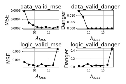
Figure 5: Metrics on Dataset A.

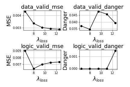
Figure 6: Metrics on Dataset B.

To generate noisy dataset, we consider a probabilistic version of Markov Decision Process (MDP) version of this state-action map: at each state the car takes the optimal action with probability $0.8$ and each other action with probability $0.1$ each. Whenever the car runs into left curb (left turn from left lane) or runs into right curb (right turn from right lane) or runs into state 2, we restart the trace from state 0.

We considered a single hidden layer neural network with 10 dimensional input $x$ as the input layer. State $i$ is represented by $\mathbbm{1}_{i}$, a vector with $1$ in $i$th position and 0s every other position. First hidden layer consists 5 neurons with sigmoid being the activation function. Next layer consists of 3 neurons with output $y$ being the softmax of these 3 neurons. Output represents the probability of each action i.e., $y(i)$ represents the probability of action $i$. The loss function considered is the cross entropy loss. We consider the constraint that car should not take left turn from left lane and right turn from right lane. In other words, if $x=1_{i}$ with $i\leq 4$ then $p(y(2))=0$ and if $x=1_{i}$ with $i>4$ then $p(y(1))=0$.

We run two sets of experiments: 1) without constraints, and 2) with constraints. As expected, when we train neural networks using unconstrained method, the model does not supress the probability of bad turns. For example, for state $0$, the model still outputs a probability of around 0.1 for left turn, which is dangerous. In the second set of experiments, we use constrained training. We can get an optimal value of the hyperparamter $\lambda$ by doing gridsearch, but in this experiment we set it to a constant value of 1.0. Our method suppresses the probability of bad turns to a low value. For example, for state $0$, the model outputs a probability of $0.0093269$. Note that this value can be reduced further by increasing $\lambda$.

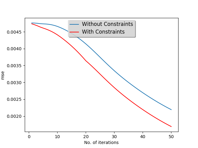
Figure 7: Convergence rate on Dataset A

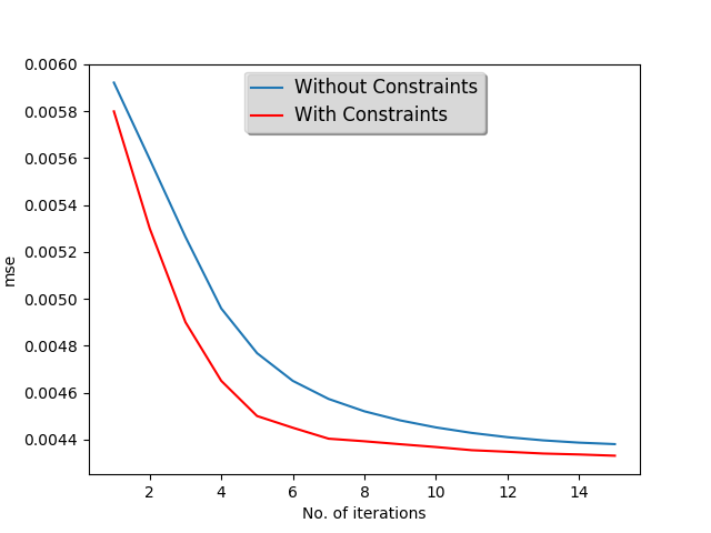
Figure 8: Convergence rate on Dataset B

5.2.2 TORCS experiment

We also ran experiments on the TORCS datasets A and B. We fit a neural network to learn the function from sensorial data to steering angle, using a single hidden layer neural network with sensorial data from past 2 seconds as input, 10 hidden nodes and sigmoid as the activation function and output being the steer angle. We consider mean square error (MSE) as the loss function. We consider the same safety constraints that were used in the logic head of the multi-headed TNN model in the previous experiment. Here, the training data is not too noisy to result in dangerous steering angle but we still show that constraints can help in reaching optimal faster.

As shown in Figs. 8 and 8, the MSE of the constrained method is less than that of the unconstrained one, and it also converges faster. Note that because of the more noisy nature of Dataset B, the MSE for it does not converge to 0.

6 Conclusion and Future Work

We introduced Trusted Neural Networks (TNNs), where we investigated two methods of incorporating logical constraints into neural networks. We demonstrated that TNNs enable higher trustworthiness in deep learning systems, and can improve efficiency of training. Specifically, we demonstrated these benefits using data generated with the open-source TORCS 3D car simulator. The novelty of TNN is not in designing a new model – the novelty is in using the multi-headed architecture for getting safety-aware ML predictions, and in using the proximal updates for getting faster convergence in this constrained setting.

Future directions of research in this vein can include application of TNNs to other high-consequence domains such as healthcare and industrial control. We would also like to theoretically study the practical limits of trustworthiness achievable with TNN models, e.g., focus on deriving bounds on the generalization error for constrained functions that can be represented by the TNN models.

References

- [1] M. Abadi, A. Agarwal, P. Barham, E. Brevdo, Z. Chen, C. Citro, G. S. Corrado, A. Davis, J. Dean, M. Devin, et al. Tensorflow: Large-scale machine learning on heterogeneous distributed systems. arXiv preprint arXiv:1603.04467, 2016.
- [2] D. Bagnall. Author identification using multi-headed recurrent neural networks. CoRR, abs/1506.04891, 2015.
- [3] A. Bar-Hillel, T. Hertz, N. Shental, and D. Weinshall. Learning a Mahalanobis metric from equivalence constraints. JMLR, 6, 2005.
- [4] D. P. Bertsekas. Constrained Optimization and Lagrange Multiplier Methods (Optimization and Neural Computation Series). Athena Scientific, 1996.
- [5] S. Boyd, N. Parikh, E. Chu, B. Peleato, and J. Eckstein. Distributed optimization and statistical learning via the alternating direction method of multipliers. Foundations and Trends® in Machine Learning, 3(1):1–122, 2011.
- [6] O. Cameron. Challenge #2: Using deep learning to predict steering angles. https://medium.com/udacity/challenge-2-using-deep-learning-to-predict-steering-angles-f42004a36ff3, September 2016.
- [7] P. L. Combettes and J.-C. Pesquet. Proximal splitting methods in signal processing. In Fixed-point algorithms for inverse problems in science and engineering, pages 185–212. Springer, 2011.
- [8] T. G. Dietterich. Constraint Propagation Techniques for Theory-driven Data Interpretation (Artificial Intelligence, Machine Learning). PhD thesis, Stanford University, 1985.
- [9] J. Duchi and Y. Singer. Efficient online and batch learning using forward backward splitting. Journal of Machine Learning Research, 10(Dec):2899–2934, 2009.
- [10] S. D. Flåm and A. S. Antipin. Equilibrium programming using proximal-like algorithms. Mathematical Programming, 78(1):29–41, 1996.
- [11] S. Ghosh, P. Lincoln, A. Tiwari, and X. Zhu. Trusted machine learning: Model repair and data repair for probabilistic models. In AAAI Workshop on AI for Connected and Automated Vehicles (AICAV), 2017.
- [12] S. Hochreiter and J. Schmidhuber. Long short-term memory. Neural Comput., 9(8), 1997.
- [13] Z. Hu, X. Ma, Z. Liu, E. H. Hovy, and E. P. Xing. Harnessing deep neural networks with logic rules. CoRR, abs/1603.06318, 2016.
- [14] W. Kotlowski and R. Slowiński. Rule learning with monotonicity constraints. In ICML, 2009.
- [15] B. Laxton, J. Lim, and D. Kriegman. Leveraging temporal, contextual and ordering constraints for recognizing complex activities in video. In CVPR, 2007.
- [16] Y. LeCun, Y. Bengio, et al. Convolutional networks for images, speech, and time series. The handbook of brain theory and neural networks, 3361(10):1995, 1995.
- [17] B. Liu, S. Mahadevan, and J. Liu. Regularized off-policy TD-learning. In F. Pereira, C. J. C. Burges, L. Bottou, and K. Q. Weinberger, editors, Advances in Neural Information Processing Systems 25, pages 836–844, 2012.
- [18] S. Mei, J. Zhu, and J. Zhu. Robust RegBayes: Selectively incorporating first-order logic domain knowledge into Bayesian models. In ICML, 2014.
- [19] K. D. Miller and D. J. C. MacKay. The role of constraints in Hebbian learning. Neural Computation, 6(1), 1994.
- [20] V. Nair and G. E. Hinton. Rectified linear units improve restricted boltzmann machines. In ICML, 2010.
- [21] Y. Nesterov et al. Gradient methods for minimizing composite objective function. CORE Discussion Papers 2007076, Université catholique de Louvain, Center for Operations Research and Econometrics (CORE), 2007.
- [22] L. D. Raedt, T. Guns, and S. Nijssen. Constraint programming for data mining and machine learning. In AAAI, 2010.
- [23] M. Richardson and P. Domingos. Markov logic networks. In Machine Learning, 2006.
- [24] L. Serafini and A. d. Garcez. Logic tensor networks: Deep learning and logical reasoning from data and knowledge. arXiv preprint arXiv:1606.04422, 2016.
- [25] P. S. Thomas, W. C. Dabney, S. Giguere, and S. Mahadevan. Projected natural actor-critic. In C. J. C. Burges, L. Bottou, M. Welling, Z. Ghahramani, and K. Q. Weinberger, editors, Advances in Neural Information Processing Systems 26, pages 2337–2345, 2013.
- [26] G. G. Towell and J. W. Shavlik. Knowledge-based artificial neural networks. Artif. Intell., 70(1-2), Oct. 1994.
- [27] B. Wymann, C. Dimitrakakisy, A. Sumnery, and C. Guionneauz. TORCS: The open racing car simulator. 2015.