Characteristic power spectrum of the diffusive interface dynamics in the two-dimensional Ising model

Abstract

We investigate properties of the diffusive motion of an interface in the two-dimensional Ising model in equilibrium or nonequilibrium situations. We focused on the relation between the power spectrum of a time sequence of spins and diffusive motion of an interface which was already clarified in one-dimensional systems with a nonequilibrium phase transition like the asymmetric simple exclusion process. It is clarified that the interface motion is a diffusion process with a drift force toward the higher-temperature side when the system is in contact with heat reservoirs at different temperatures and heat transfers through the system. Effects of the width of the interface are also discussed.

I Introduction

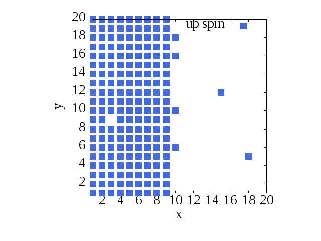
Dynamical and statistical properties of an interface between two phases have been studied in relation to various physical phenomena such as phase ordering, crystal or dendrite growth, and self-propelled droplet motion driven by surface tension gradient11 . A simple example is found in the two-dimensional Ising model with ferromagnetic interaction. Below the critical temperature , if a magnetic field in opposite directions is imposed at the left and right boundaries, there appears an interface in the vertical direction as shown in Fig. 1. If no magnetic field is applied in the bulk, the interface carries out diffusive motion, while the bulk magnetic field drives the inter face motion in one direction, which is described by the KPZ equation 1 .

Actually diffusive motion of an interface is also seen in one-dimensional systems 2 . Though no phase transitions occur in equilibrium one-dimensional systems, noneqilibrium models like the asymmetric simple exclusion process (ASEP) have the first-order phase transition where two phases coexist and an interface appears between them. One of the authors has clarified that characteristics of the diffusive motion of the interface are captured by the power spectrum that shows characteristic power law behavior with exponent $-3/2$ and the prefactor is determined by the diffusion constant, the difference of the density of two phases and the system size 3 .

In this paper, we apply the method to the two-dimensional Ising model to investigate the interface motion. In particular, we discuss the relation between the interfacial width and the power spectrum. Moreover, when the boundaries of the systems are in contact with heat reservoirs at different temperatures, we find that a drift force towards the higher temperature side is generated accompanying heat conduction. As the result, the probability of finding the interface is larger in the higher temperature region as reported by Yukawa et al. 4 .

Figure 1: Snapshot of an interface of the two-dimensional Ising model of size $20\times 20$ at the temperature $T=1.5$. Sites with up spins are filled and those with down spins are blank.

To investigate such noneqilibrium systems, use of Glauber dynamics is not appropriate because it needs a prescribed temperature value. In those cases deterministic energy-conserving dynamics such as Creutz and Q2R dynamics have been used 4 ; 5 . At low temperatures, however, those dynamics freezes and the interface hardly moves for a long time. Thus, we need to devise a new dynamics to recover diffusivity in low temperature. Such dynamics is introduce in Sec. II . We apply the new dynamics to simulate heat conduction and analyze the power spectrum. We also compare it with other time evolution rules.

The remainder of the paper is organized as follows. In Sec. III, simulation results on heat conduction with and without an interface are exhibited. In either case, the thermal conductivity is estimated. Section IV is the main part of the paper, where we review the relation between the power law in the power spectrum and diffusive motion of the interface and apply it to the Ising model in equilibrium or noneqilibrium steady states. Section V is devoted to summary and conclusion.

II Dynamics

Because the Ising model does not have its own dynamics, we have to introduce some time evolution rule. Glauber dynamics 6 is most commonly used for simulation of equilibrium states. In Glauber dynamics, temperature appears as a parameter and the realization of the equilibrium state at the temperature is guaranteed. In heat conduction, however, temperature values are given only at the boundaries and the bulk temperature is determined as the result of dynamics. Thus, the Glauber dynamics is not suitable for the simulation of heat conduction.

Figure 2: Temperature profiles generated by Creutz dynamics and KSC dynamics. The system size is $20\times 20$ and the temperature of heat reservoirs is $T_{R}=T_{L}=1.5$. Red squares (green circles) indicate the result for the system with (without) an interface obtained by average over $9\times 10^{7}$ steps after $10^{7}$ steps of transients. Blue upward triangles (purple downward triangles) indicate the result for the system with (without) an interface obtained by KSC dynamics calculated in the similar way as Creutz dynamics.

Figure 3: (a) Evolution of magnetization for $10^{6}$ time steps using Creutz dynamics in the system with an interface. System size is $20\times 20$ and the temperature of heat reservoirs is $T_{R}=T_{L}=1.5$. (b) Evolution of magnetization by KSC dynamics in the system with interface obtained in the similar system size and at the similar temperature as by Creutz dynamics.

Creutz devised an alternative dynamics for the Ising model. In the case of the square lattice, it is a dynamics that conserves the following Hamiltonian 5 ; 7

$$H=-\sum_{i,j}(\sigma_{i,j}\sigma_{i+1,j}+\sigma_{i,j}\sigma_{i,j+1})+\sum_{i,j}4\tilde{\sigma}_{i,j},$$ (1)

where $\sigma_{i,j}\in\{-1,+1\}$ denotes the Ising spin on site $(i,j)$ and $\tilde{\sigma}_{i,j}\in\{0,1,2,3\}$ is an auxiliary variable called “momentum.” The first term means the usual ferromagnetic interaction and the second term is a kind of “kinetic energy.” In each step, spin $\sigma_{i,j}$ flips if and only if the change of the interaction energy can be compensated by some change of momentum variable $\tilde{\sigma}_{i,j}$. The condition is given by

$$0\leq\tilde{\sigma}_{i,j}-\frac{1}{2}\sigma_{i,j}(\sigma_{i-1,j}+\sigma_{i+1,j}+\sigma_{i,j-1}+\sigma_{i,j+1})\leq 3$$ (2)

and when it is satisfied, $\sigma_{i,j}$ changes its sign and $\tilde{\sigma}_{i,j}$ becomes ${\tilde{\sigma}_{i,j}}^{\prime}=\tilde{\sigma}_{i,j}-\frac{1}{2}\sigma_{i,j}(\sigma_{i-1,j}+\sigma_{i+1,j}+\sigma_{i,j-1}+\sigma_{i,j+1})$. If we divide the lattice into two sublattices just as white and black fields of the chessboard, the Creutz dynamics can be carried out simultaneously for spins on a sublattice chosen alternatingly. Then, the dynamics is fully deterministic. An alternative way is to choose a site randomly and examine if its spin can be flipped. In the following the latter is employed. A simplified variant of Creutz dynamics is Q2R, where the “kinetic energy”term is absent and spins can flip only if the sum of the four nearest-neighbor spins is zero.

In an isolated system, the total energy is conserved under Creutz or Q2R dynamics and the system reaches equilibrium in a long run, provided that the dynamics is sufficiently ergodic. Attachment of heat reservoirs to parts of the system is straightforward. We only have to make spins in contact with heat reservoirs evolve according to Glauber dynamics. The temperature of the left heat reservoir is $T_{L}$ and that of the right heat reservoir is $T_{R}(\leq T_{L})$. Note that we employ an energy unit where Boltzmann constant is unity. Thus, the critical temperature of the two-dimensional Ising model is $T_{c}=2/\log(1+\sqrt{2})$. Thus, we can simulate heat conduction using such dynamics5 . Moreover, if both $T_{L}$ and $T_{R}$ are below $T_{c}$ and $+$ spin is fixed at the boundary of the left reservoir and $-$ spin is fixed at the boundary of the right reservoir, an interface is formed. Because momentum variables are expected to obey the canonical distribution in local equilibrium states, local temperature can be estimated by measuring the momentum distribution.

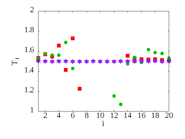
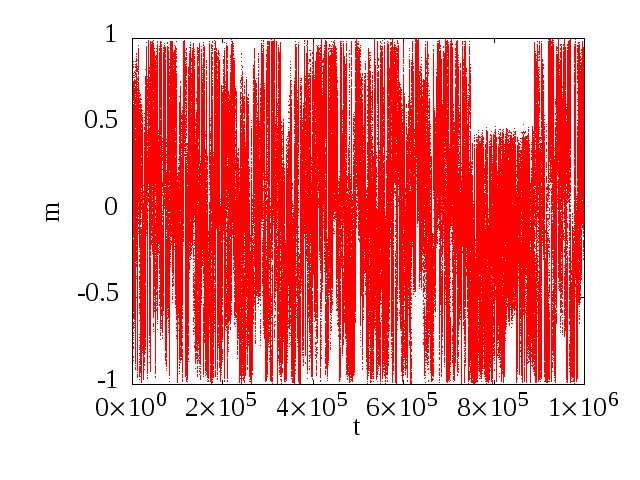
At low temperature, however, Creutz and Q2R dynamics share a common problem. Below the critical temperature, most spins orient in the same direction. Thus, large momentum is necessary to compensate energy increase brought by a spin flip. However, there are few large momentum in low temperature and accordingly the dynamics freezes. Figure 2 shows the temperature profile after large time steps by Creutz dynamics with two heat reservoirs, both at temperature $1.5$, where the system does not reach equilibrium at uniform temperature in simulation time. In 5 , it is reported that the thermal conductivity drops abruptly below the critical temperature in the case of no fixed spins at the boundaries. When an interface is present, the magnetization is stuck and the diffusive motion of an interface is subdued as seen in Fig. 3.

A solution to this problem was brought by Casartelli et al. 8 . They studied Q2R and noticed the same problem. Then they modified Q2R by adding a new rule of spin flip to it. It is called Kadanoff-Swift (KS) dynamics, where a pair of next nearest-neighbor spins exchange their values if energy is unchanged by the exchange. It should be noted that the Hamiltonian does not include next-nearest-neighbor coupling. Such spins are only dynamically coupled. To measure local temperature in nonequilibrium systems, we apply the same modification to Creutz dynamics and we call the resultant dynamics Kadanoff-Swift-Creutz (KSC) dynamics.

Precisely, the algorithm that we employ for our KSC dynamics is the following.

1. Choose random Creutz dynamics or KS dynamics.

2. In the former case, a site is randomly chosen and its spin is updated according to Creutz dynamics. In the latter case, a couple of nearest-neighbor sites are randomly chosen and the spins are updated according to KS dynamics.

3. Repeat 1 and 2 $L_{x}L_{y}$ times, where $L_{x}$ and $L_{y}$ are the horizontal and vertical size of the system.

4. Update the spins in contact with reservoirs according to Glauber dynamics.

5. Repeat the procedure from 1 to 4, which is counted as a unit of time.

In this dynamics, relaxation to an equilibrium state at uniform temperature is realized as seen in Fig. 2 even at a temperature considerably below the critical temperature. Moreover, Fig. 3 shows that the magnetization changes smoothly from $-1$ to $1$.

III Thermal conductivity

First we examine how the new dynamics and the existence of an interface affect Fourier’s law and the thermal conductivity. We have carried out numerical simulation for the system of size $40\times 40$, both horizontal ends of which are in contact with heat reservoirs at different temperatures with difference $\Delta T=T_{L}-T_{R}$. The time evolution of the system is governed by the KSC dynamics. Then the temperature gradient is formed in the system as in the Creutz dynamics 5 ; 7 . As we see in Fig. 4, heat flux $J$ is proportional to the temperature difference $\Delta T$ irrespective of the existence or nonexistence of an interface.

Figure 4: Heat flux in the system with and without an interface. The system size is $40\times 40$ and the average temperature of heat reservoirs is $T_{\mathrm{ave}}=1.0,1.5,2.0$. Data is obtained from averaging over 50 samples for $4.5\times 10^{7}$ steps each. Red (filled squares), green (filled circles) and blue dots (filled triangles) indicate the results of $T_{\mathrm{ave}}=1.0$, $1.5$, and $2.0$, respectively, in the system with an interface and light red (open squares), light blue (open circles), and yellow dots (open triangles) indicate those of $T_{\mathrm{ave}}=1.0,1.5$, and $2.0$, respectively, in the system without an interface.

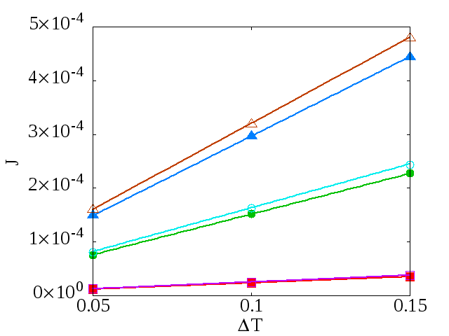
However, values of the thermal conductivity show difference between the two cases. The thermal conductivity is defined as

$$\kappa(T)=J\frac{L_{x}}{\Delta T}.$$ (3)

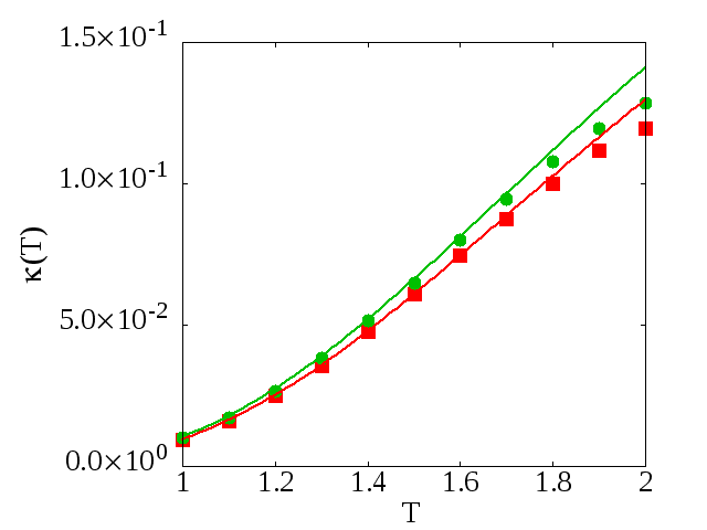
Figure 5 shows the thermal conductivity in the system with KSC dynamics. In low temperature, the thermal conductivity varies like $\kappa\sim\frac{1}{T^{2}}\exp(-\frac{8}{T})$ irrespective of the presence or absence of an interface, as was suggested in 5 . In the case of the KSC dynamics, the thermal conductivity is larger in the system without an interface than in that with an interface. Interestingly, the converse is the case when the Creutz dynamics is employed.

Figure 5: Thermal conductivity $\kappa(T)$ by KSC dynamics. Red squares and green circles indicate the results of the system with and without an interface respectively. Red (lower) and green (upper) lines indicate $28.3/T^{2}\exp(-8/T)$ and $30.8/T^{2}\exp(-8/T)$ respectively.

Figure 6: (a) Contribution from Creutz dynamics to the thermal conductivity, $\kappa_{c}(T)$. Red squares and green circles indicate the results of the system with and without an interface respectively. (b) Contribution from KS dynamics to the thermal conductivity, $\kappa_{k}(T)$. Red squares and green circles indicate the results of the system with and without an interface respectively.

Figure 7: Example of spin configuration. Panel (a) is the case where the two opposite spins are adjacent at an interface. Panel (b) is the case where the two opposite spins are not adjacent at an interface.

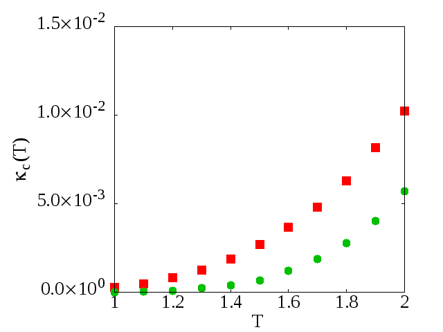
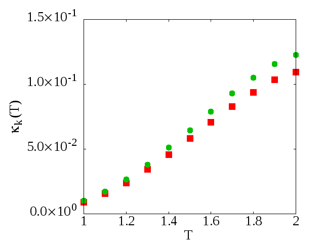
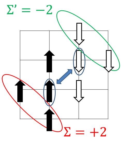
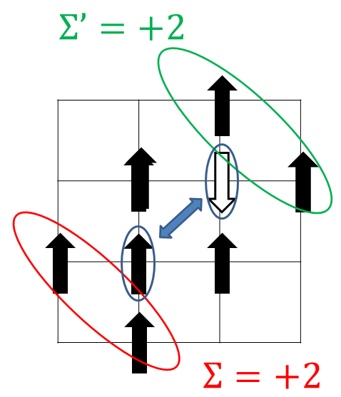
Let us divide heat flux $J$ into contribution from Creutz dynamics $J_{c}$ and that from KS dynamics $J_{k}$. We defined $\kappa_{c}$ and $\kappa_{k}$ as thermal conductivity computed using $J_{c}$ and $J_{k}$, respectively. As Figs. 6 and 6 show, $\kappa_{c}$ becomes larger while $\kappa_{k}$ becomes smaller when an interface is present. The reason for this is explained as follows. The condition of flip in Creutz dynamics depends on change of spin-interaction energy by the flip. Because spins of different signs are adjacent at an interface, a spin flip can occur with a small change of energy there. If there is no interface, a spin is likely to be surrounded by spins of the same sign and large energy is necessary to flip. Thus Creutz dynamics contributes more in conducting energy when an interface exists. On the contrary, KS dynamics is suppressed near an interface. Consider a pair of next-nearest-neighbor spins at a flat interface as shown in Fig. 7. If they exchange their signs, interaction energy with the spins marked $\Sigma$ and $\Sigma^{\prime}$ changes and the total energy increases by 8. Thus it is inhibited. Apart from an interface, if only one spin is surrounded by opposite spins, it can exchange its sign with a next-nearest-neighbor spin without change of energy. Thus the presence of an interface controls the KS dynamics and makes $\kappa_{k}$ smaller.

IV probability distribution of the interface position

We define the interface position by using magnetization $m=(L_{x}L_{y})^{-1}\sum_{i,j}\sigma_{i,j}$ as

$$X=\frac{L_{x}}{2}(m+1).$$ (4)

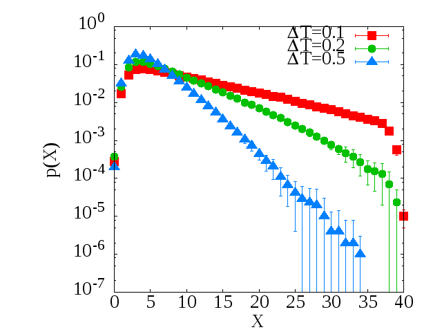
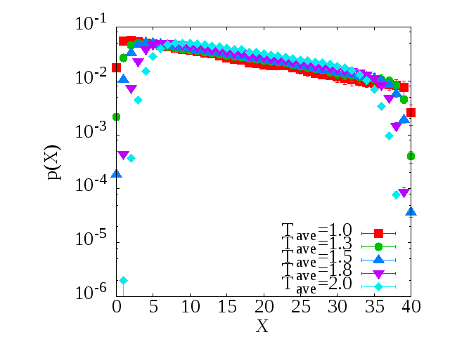
Thus, the interface position is at the left edge $X=0$ if $m=-1$, at the right edge $X=L_{x}$ if $m=+1$, and in the center if $m=0$. We numerically estimate the probability distribution of the interface position in the system of size 40$\times$40 with KSC dynamics and heat reservoirs. Figure 8 is the result for $T_{\mathrm{ave}}=1.5$ and various $\Delta T$, which shows that the interface prefers to exist in the high temperature region. The distribution is roughly exponential and the tendency is stronger with larger $\Delta T$. The result agrees with 4 , where Creutz dynamics is employed, though. The exponential distribution is more evident when $\Delta T$ is small as seen in Fig. 8.

We notice that the decay of $p(X)$ close to the boundary is faster for higher temperatures. It is explained as follows. The magnetization on the right (left) end is fixed to $+1$ ($-1$) by the boundary condition. Because its magnitude is larger than the spontaneous magnetization at temperature $T_{L}$ or $T_{R}$, the interface cannot approach the very ends. The movable range of the interface is smaller than $[L^{\prime}/2,L_{x}-L^{\prime}/2]$, where $L^{\prime}$ denotes the width of the interface. Because the width of the interface is greater for higher temperatures, the movable range is smaller. As is discussed later, the change of the effective system size plays an role in the temperature dependence of the power spectrum.

Figure 8: (a) Probability distribution of the interface position in KSC dynamics with heat reservoirs whose average temperature is $T_{\mathrm{ave}}=1.5$ and $\Delta T=0.1,0.2$, and $0.5$. (b) Probability distribution of the interface position when $\Delta T=0.05$ and $T_{\mathrm{ave}}=1.0$, 1.3, 1.5, 1.8, and 2.0.

Figure 9: Interface energy estimated by using Eq.(7) from the probability distribution.

Actually the exponential distribution is verified on the assumption of local equilibrium as follows. The local equilibrium means that we can represent the probability distribution using temperature $T(x)$ and as

$$p(X)\sim\exp\left(-\frac{\sigma(T,L_{y})}{T(X)}\right),$$ (5)

where $\sigma(T,L_{y})$ is the interface energy at $T$. If $\Delta T$ is very small, $1/T(x)$ can be approximated as

$$\frac{1}{T(x)}\sim\frac{1}{T_{\mathrm{ave}}}\left(1+\frac{\Delta T}{T_{\mathrm{ave}}}\frac{x}{L}\right)$$ (6)

and $\sigma(T,L_{y})$ is regarded as a constant. Then, the probability distribution becomes

$$p(X)\sim\exp\left(-\sigma(T_{\mathrm{ave}},L_{y})\frac{\Delta T}{{T_{\mathrm{ave}}}^{2}}\frac{X}{L}\right).$$ (7)

The interface energy $\sigma(T,L_{y})$ thus estimated is shown in Fig. 9.

V property of the power spectrum induced by the diffusive motion of interface in two dimensional Ising model.

V.1 Relationship between the power spectrum and the diffusive motion of the interface

Let us briefly review the relation between the power spectrum and the diffusive motion of an interface according to 3 . Consider a one-dimensional system of size $L$, where the left part is in one phase of density $\rho_{-}$ and the right part is in the other phase of density $\rho_{+}(>\rho_{-})$ and an interface at position $x(t)$ divides the two phases. In this case, the density at site $y$ ($\rho_{y}(t)$) is described as

$$\rho_{y}(t)=\rho_{-}+(\rho_{+}-\rho_{-})\theta(y-x(t)),$$ (8)

where $\theta(x)$ is the step function. Now let us assume that $x(t)$ executes Brownian motion with diffusion constant $D$. Then, the probability density of finding the interface at $x$ obeys the diffusion equation.

$$\frac{\partial P}{\partial t}=D\frac{\partial^{2}P}{\partial x^{2}}.$$ (9)

Under the reflecting boundary condition

$$\frac{\partial P(x,t)}{\partial x}=0$$ (10)

at $x=0$ and $L$, the stationary state is $P_{st}(x)=L^{-1}$ and the transition probability is

$$P(x,t|x_{0},t_{0})=\frac{1}{L}+\frac{2}{L}\sum_{n=1}^{\infty}e^{-D\lambda_{n}^{2}t}\cos\lambda_{n}x\cos\lambda_{n}x_{0},$$ (11)

where $\lambda_{n}=\frac{n\pi}{L}$. Then the autocorrelation function of $\delta\rho_{y}(t)=\rho_{y}(t)-\langle\rho_{y}\rangle_{st}$ is obtained as

$$\langle\delta\rho_{y}(t)\delta\rho_{y}(0)\rangle=\frac{2(\rho_{+}-\rho_{-})^{2}}{L^{2}}\sum_{n=1}^{\infty}\frac{e^{-D\lambda_{n}^{2}|t|}}{\lambda_{n}^{2}}\sin^{2}\lambda_{n}y.$$ (12)

Thanks to the Wiener-Khinchin theorem, the power spectral density is given by the Fourier transform of the correlation function, which is calculated as

$$I(\omega) = \int_{-\infty}^{\infty}e^{-i\omega t}\langle\delta\rho_{y}(t)\delta\rho_{y}(0)\rangle dt$$ (13)

$$= \frac{2(\rho_{+}-\rho_{-})^{2}}{L^{2}}\sum_{n=1}^{\infty}\frac{2D}{D^{2}\lambda_{n}^{4}+\omega^{2}}\sin^{2}\lambda_{n}y$$

If we assume $y=L/2$ and large $L$, the sum can be replaced by an integral which is evaluated using the residue calculus. Thus we arrive at

$$I(\omega)=(\rho_{+}-\rho_{-})^{2}\frac{\sqrt{2D}}{2L}\omega^{-1.5}.$$ (14)

To extend the above relation to the two-dimensional Ising model, we consider the following two types of sequences and their power spectrum. One is the power spectrum of a temporal sequence of column-averaged magnetization

$$\{s_{i}(t)=\frac{1}{L_{y}}\sum_{j}\sigma_{i,j}(t)|t=0,1,2,...,T-1\}.$$ (15)

In our simulations, the length of the sequence is $T=2^{20}$. Fourier components of the sequence (15) are computed as

$$S_{n}=\sum_{t=0}^{T-1}s_{i}(t)\exp(-\omega_{n}t)$$ (16)

where $\omega_{n}=\frac{2\pi n}{T}$. Then, the power spectrum $I(\omega)$ is derived as

$$I(\omega_{n})=T\langle{|S_{n}|^{2}}\rangle,$$ (17)

where the brackets mean averaging over 200 samples. If the interface behaves as normal diffusion with diffusion constant $D$, we expect to obtain the power spectrum of the form (14) with replacement of $\rho_{+}-\rho_{-}$ with $2m_{0}$, where $m_{0}$ is the spontaneous magnetization9

$$m_{0}(T)=[1-\sinh(2/T)^{-4}]^{1/8}.$$ (18)

The other is for a temporal sequence of spin values of a site $\{\sigma_{i,j}(t)|t=0,1,2,\dots,T-1\}$. Its power spectrum is defined in the same manner as above.

V.2 Equilibrium System with Glauber dynamics

Figure 10: (a) Power spectra for $\sigma_{L_{x}/2,L_{y}/2}(t)$ and $s_{L_{x}/2}(t)$ in the system of $L_{x}=L_{y}=40$ at $T=2.0$. Red (upper) dots indicates the former and green (lower) dots the latter. Blue line indicates $-1.5$ power law. (b) Plot of $I(\omega)L_{x}$ vs $\omega$ for $L_{x}=40$ [red (lower)], 80 [green (middle)], and 100 [blue (upper)] for the power spectrum of $s_{L_{x}/2}(t)$. The data collapse shows the $L_{x}$ dependence of Eq. (17)

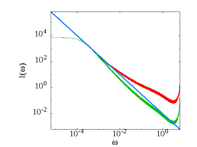
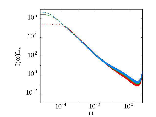
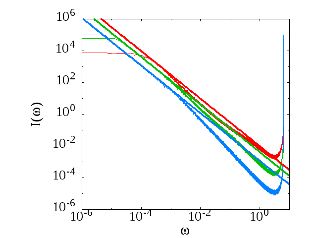
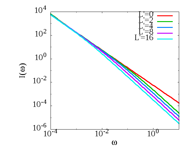
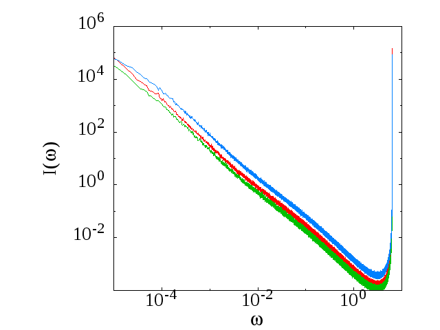
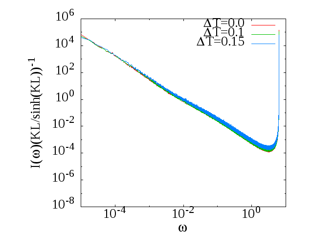
First we examine the power spectra in the two-dimensional Ising model with Glauber dynamics. Figure 10 shows the power spectrum at $T=2.0$ slightly lower than the critical temperature $T_{c}$. As the figure shows, both the power spectra of the sequence of a spin on site ($\sigma_{L_{x}/2,L_{y}/2}(t)$) and the column-averaged magnetization at $L_{x}/2$ ($s_{L_{x}/2}(t)$) show power-law behavior with exponent $-1.5$ in a range of low frequencies. Moreover, Fig. 10 shows data collapse for horizontal-size variation according to Eq. (14). These results indicate that the interface undergoes normal diffusion in a certain time scale. Furthermore, temperature dependence of the power spectra shown in Fig. 11 indicates that the diffusion constant becomes smaller as temperature decreases.

Figure 11: Temperature dependence of the power spectra of $s_{L_{x}/2}(t)$ ($L_{x}=L_{y}=40$). Red (upper), green (middle), and blue (lower) dots indicate the results for $T=2.0$, $1.0$, and $0.5$, respectively. Red (upper), green (middle), and blue (lower) lines indicate $-1.5$ power law at $T=2.0$, $1.0$, and $0.5$, respectively.

Figure 12: Power spectra described by Eq. (23) for a variety of width $L^{\prime}$.

Figure 13: Mean square displacement of Eq.(24) ($L=0.01,L=50$).

Figure 14: Profile of column-averaged magnetization fitted by tanh profile Eq. (25). Red squares indicate the numerical result at $T=1.5$ and green line indicates $-0.99\tanh(2/4.22(i-i_{0}))$.

However, the power-law behavior is limited to a short range of low frequencies and the graph shows a characteristic curve in a higher frequency region. In the case of the power spectrum of column-averaged magnetization $s_{L_{x}/2}(t)$, the deviation is explained by taking into account width of the interface. In the one-dimensional case, an instantaneous density profile is a step function without a width. Contrastingly, the column-averaged magnetization has a width. Thus we have to consider its influence on the spectrum. In place of the step-function profile, let us assume that the $s_{x}(t)$ is approximately described as

$$s_{x}(t)=\begin{cases}m_{0}&(0\leq x<{X(t)-\frac{L^{\prime}}{2}})\\ \frac{2m_{0}}{L^{\prime}}(x-X(t))&({X(t)-\frac{L^{\prime}}{2}}\leq x<{X(t)+\frac{L^{\prime}}{2}})\\ -m_{0}&({X(t)+\frac{L^{\prime}}{2}}\leq x\leq L)\end{cases}$$ (19)

where $L^{\prime}$ denotes the width and $X(t)$ is the position of the interface at time $t$, which undergoes Brownian motion with diffusion constant $D$. In this case the autocorrelation function of $\delta s_{y}(t)=s_{y}(t)-\langle s_{y}\rangle_{st}$ is calculated as

$$\langle\delta s_{y}(t)\delta s_{y}(0)\rangle=\frac{8m_{0}^{2}}{L^{2}}\sum_{n}e^{-D\lambda_{n}^{2}|t|}\frac{\sin^{2}(\frac{L^{\prime}}{2}\lambda_{n})}{(\frac{L^{\prime}}{2}\lambda_{n})^{2}}\frac{\sin^{2}{\lambda_{n}y}}{\lambda_{n}^{2}},$$ (20)

where $\lambda_{n}=n\pi/L$, and the power spectral density is its Fourier transform

$$I(\omega) = \int_{-\infty}^{\infty}\exp(-i\omega t)\langle{\delta s_{y}(t)\delta s_{y}(0)}\rangle dt$$ (21)

$$= \frac{16Dm_{0}^{2}}{L^{2}}\sum_{n=1}^{\infty}\frac{\sin^{2}(\frac{L^{\prime}}{2}\lambda_{n})}{(\frac{L^{\prime}}{2}\lambda_{n})^{2}}\frac{\sin^{2}{\lambda_{n}y}}{D^{2}\lambda_{n}^{4}+\omega^{2}}.$$

Putting $y=L/2$ and assuming that $L$ is large, the sum over $n$ can be replaced by the following integral

$$I_{E}(\omega)\sim\frac{32m_{0}^{2}}{\pi DL}\int_{0}^{\infty}\left(\frac{\sin\beta x}{\beta x}\right)^{2}\frac{dx}{x^{4}+\alpha^{2}},$$ (22)

where $\alpha=\frac{\omega}{D}$ and $\beta=\frac{L^{\prime}}{2}$.

This integral is evaluated using residue calculus and we arrive at

$$I_{E}(\omega)=(2m_{0})^{2}\left[\frac{2D^{\frac{3}{2}}}{LL^{\prime 2}}\omega^{-\frac{5}{2}}\left\{\exp(-L^{\prime}(\frac{\omega}{2D})^{\frac{1}{2}})\cos(L^{\prime}(\frac{\omega}{2D})^{\frac{1}{2}}+\frac{\pi}{4})-\frac{1}{\sqrt{2}}\right\}+\frac{2D}{LL^{\prime}}\omega^{-2}\right].$$ (23)

Figure 12 shows $I_{E}(\omega)$ for various values of width $L^{\prime}$. They obey the power law with exponent $-1.5$ in a low-frequency region but the slope becomes steeper beyond a certain value that is a decreasing function of the width.

To compare Eq. (23) with the numerically obtained power spectra, we need the diffusion constant $D$ and the width of the interface $L^{\prime}$. Moreover, because the boundary condition is different, we treat the system size $L$ as a fitting parameter.

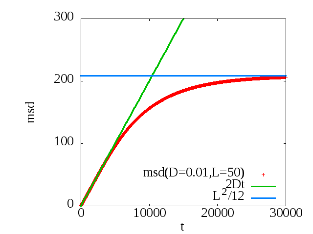
The diffusion constant and the effective system size are numerically estimated as follows. We prepare a system with a straight interface at $x=L/2$ and measure the evolution of the mean square displacement (msd), which is analytically derived as

$$\langle(X-L/2)^{2}\rangle=\sum_{k=1}\frac{L^{2}}{\pi k^{2}}\{\exp(-\frac{4\pi^{2}Dk^{2}}{L^{2}}t)-1\}(-1)^{k}$$ (24)

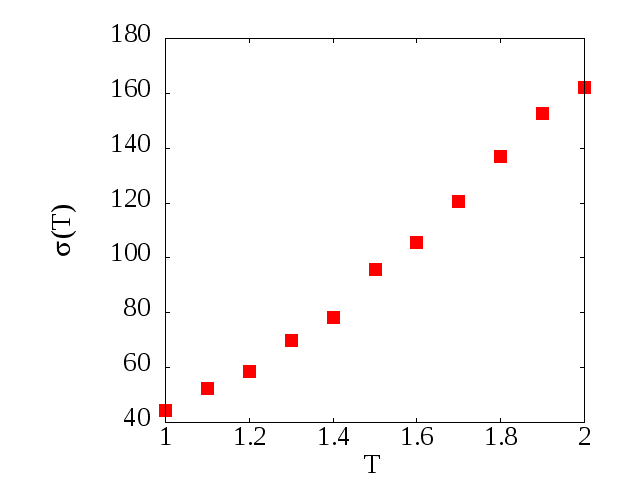
As Fig. 13 shows, the msd behaves like $2Dt$ for small $t$ and converges to $L^{2}/12$ for large enough $t$. The numerical results thus obtained indicate that $L\simeq L_{x}$ at small temperature, while $L$ becomes smaller than $L_{x}$ at higher temperature.

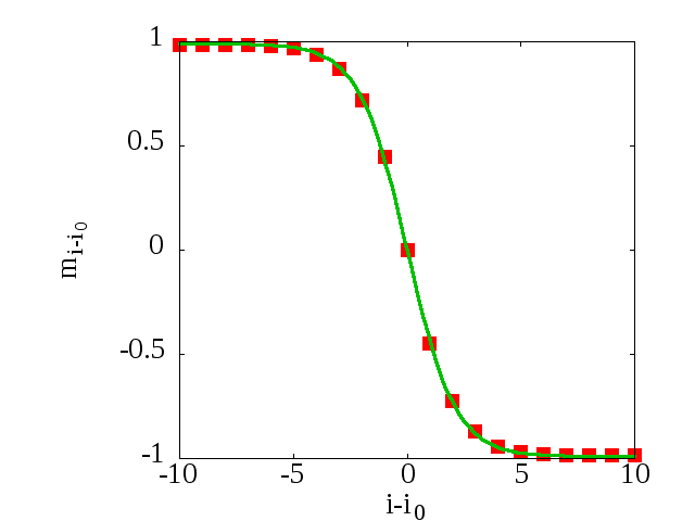
The interfacial width $L^{\prime}$ is estimated by fitting the profile of column-averaged magnetization $s_{i}(t)$. Given a profile $s_{i}(t)$ at time $t$, we determine the interface position $i_{0}(t)$ as the position that gives minimum $|s_{i}(t)|$. Then the time average of $s_{i-i_{0}(t)}(t)$ is well fitted by the function

$$-m_{0}\tanh(2i/L^{\prime}),$$ (25)

as shown in Fig. 14. For example, at $T=1.5$, $L^{\prime}$ is estimated to be 4.22 as shown in Fig. 14.

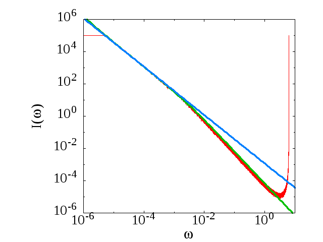
Figures 15 and 15 show comparison between the power spectrum of $s_{L_{x}/2}$ and $I_{E}(\omega)$ at $T=2.0$ (Fig. 15) and $T=0.5$ (Fig. 15). Compared with Fig. 10, we can see that $I_{E}(\omega)$ better fits the observed power spectrum than the mere $-1.5$ power law does. Thus the time evolution of an interface in equilibrium Glauber dynamics is normal diffusion of an interface having width. The fit is better as temperature decreases. Thus we have confirmed that $I_{E}(\omega)$ reproduces the power spectrum of $s_{L_{x}/2}$ in frequency range $(\omega<0.01)$ at $T=2.0$ and that in a wider frequency range $(\omega<1.0)$ at $T=0.5$. The magnitude of the power spectrum is larger at higher temperature. This is mainly because the diffusion constant is larger in higher temperature and the effective system size is smaller in higher temperature as discussed before. Difference in the spontaneous magnetization is not significant except near the critical temperature. Deviation seen in high-frequency range at $T=2.0$ is due to approximation in the employed profile Eq. (19) and fluctuations around the mean profile in Fig.14.

Figure 15: Comparison between the power spectrum of $s_{L_{x}/2}$ and $I_{E}(\omega)$ for the system of size $L_{x}=L_{y}=40$ and temperature (a) $T=2.0$ and (b) $T=0.5$. In both figures, red dots indicate the numerically obtained power spectrum of $s_{L_{x}/2}$, green a little curved line shows $I_{E}(\omega)$ with (a) $D=0.0158,L=29.9,L^{\prime}=7.4,m_{0}=0.90$ and (b) $D=0.000272$, $L=40.0,L^{\prime}=0.8,m_{0}=1.00$, and blue straight line is a guide to the eyes for the power law with exponent $-1.5$.

V.3 Equilibrium system with the KSC dynamics

In equilibrium systems, results from the KSC dynamics do not much differ from the Glauber case, though the diffusion constant is different from that for the Glauber dynamics at the same temperature. Figure 16 shows the comparison between the numerically obtained power spectrum and Eq. (23). The low frequency region shows a good agreement between them.

Figure 16: Comparison between the numerically obtained power spectrum of $s_{L_{x}/2}$ from the KSC dynamics and $I_{E}(\omega)$ for the system of size $L_{x}=L_{y}=40$. Red (upper) and green (lower) dots show the power spectrum at $T=2.0$ and $1.0$, respectively. Red (upper) and green (lower) lines indicate $I_{E}(\omega)$ for $T=2.0$ ($D=0.00491,L=29.0,L^{\prime}=7.3$) and $T=1.0$ ($D=0.000569,L=39.3,L^{\prime}=2.4$), respectively.

V.4 Nonequilibrium system

We consider the case where the system is attached to two reservoirs at different temperatures $T_{L}$ and $T_{R}$. We assume that $T_{L}>T_{R}$ and states in the bulk of the system are updated by the KSC dynamics. As mentioned before, in nonequilibrium cases the stationary probability distribution of the interface position is exponential. This is realized by adding a constant drift term to the Fokker-Planck equation as follows.

$$\frac{\partial P}{\partial t}=\frac{\partial}{\partial x}(-FP+D\frac{\partial P}{\partial x}),$$ (26)

where $F$ is a constant representing the force exerted on the interface. The reflecting boundary condition in this case is

$$\left(-FP+D\frac{\partial P}{\partial x}\right)\Big{|}_{x=0,L}=0.$$ (27)

From Eqs. (26) and (27), we derive the stationary distribution as

$$P_{\mathrm{st}}(x)=\frac{Ke^{-KL}}{\sinh(KL)}\exp(2Kx),$$ (28)

where $K=\frac{F}{2D}$. Thus we obtained an exponential distribution.

Figure 17: Drift force $F$ estimated from the probability distribution. The system size is $40\times 40$ and the average temperature $T_{\mathrm{ave}}=1.0,1.5,2.0$. Red squares, green circles, and blue triangles indicate the results for $T_{\mathrm{ave}}=1.0,1.5$ and $2.0$, respectively. Red (lower), green (middle), and blue (upper) lines are fitting lines, $0.000512\Delta T,0.00203\Delta T$, and $0.00464\Delta T$, respectively. To calculate the probability distribution to estimate the drift force $F$, $4.5\times 10^{7}$ steps are taken after transient of $5\times 10^{6}$ steps.

We examine whether Eq. (26) can also explain dynamical properties of the interface. The power spectrum for the time sequence of the column-averaged magnetization at a horizontal position is derived in the same manner as before, which results in

$$I_{NE}(\omega) =(2m_{0})^{2}\frac{2}{DLL^{\prime 2}}\frac{KL}{\sinh(KL)}\left(\frac{\omega}{D}\right)^{-2}\frac{\sqrt{\sqrt{(K^{2})^{2}+(\frac{\omega}{D})^{2}}+K^{2}}}{\sqrt{(K^{2})^{2}+(\frac{\omega}{D})^{2}}}\left[-\frac{1}{\sqrt{2}}\cosh(KL^{\prime})\right.$$

$$+\exp\left(-L^{\prime}\sqrt{\frac{\sqrt{(K^{2})^{2}+(\frac{\omega}{D})^{2}}-K^{2}}{2}}\right)\left\{\frac{1}{\sqrt{2}}\cos\left(L^{\prime}\sqrt{\frac{\sqrt{(K^{2})^{2}+(\frac{\omega}{D})^{2}}-K^{2}}{2}}\right)\right.$$

$$\left.-\left(\frac{\omega}{D}\right)^{-1}\left(\sqrt{(K^{2})^{2}+(\frac{\omega}{D})^{2}}-K^{2}\right)\sin\left(L^{\prime}\sqrt{\frac{\sqrt{(K^{2})^{2}+(\frac{\omega}{D})^{2}}-K^{2}}{2}}\right)\right\}$$

$$+\left.\left(\frac{\sqrt{\sqrt{(K^{2})^{2}+(\frac{\omega}{D})^{2}}+K^{2}}}{\sqrt{(K^{2})^{2}+(\frac{\omega}{D})^{2}}}\right)^{-1}L^{\prime}\left(\frac{\sinh(KL^{\prime})}{KL^{\prime}}\right)\right].$$ (29)

Details of the derivation is given in Appendix A.

When $K\to 0$, it converges to $I_{E}(\omega)$. If $|K|D\ll\omega$ and $|K|L^{\prime}\ll 1$, we have

$$I_{NE}(\omega)\sim\frac{KL}{\sinh(KL)}I_{E}(\omega).$$ (30)

Figure 18: Comparison between the simulation results for the power spectra of $s_{L_{x}/2}$ ($T=1.0,L_{x}=L_{y}=40$) and $I_{NE}(x)$. Red (upper), green (middle), and blue (lower) dots indicate the numerical results for $\Delta T=0.0$, $0.1$ and $0.15$. Dark red (upper), dark green (middle), and dark blue (lower) lines show corresponding $I_{NE}(x)$ for the same color. Other parameter values are $D=0.000569$, $L=39.3$, $L^{\prime}=2.4$, and $F=0.000512\Delta T$.

Figure 19: Comparison between the power spectra of $s_{L_{x}/2}$ for the system of size $L_{x}=L_{y}=40$ in equilibrium [$T=1.0$, red (middle) dots] and in nonequilibrium [$T_{\mathrm{ave}}=1.0$, $\Delta T=0.1$, green (lower) dots)]. Blue (upper) dots represent the power spectrum of $s_{X_{h}}$ in nonequilibrium system ($T=1.0$, $\Delta T=0.1$, $X_{h}=7$).

Figure 20: Scaling of the power spectra of $s_{L_{x}/2}$ ($T=1.0,L_{y}=40$). The vertical axis is $I(\omega)(\frac{KL}{\sinh(KL)})^{-1}$. They are scaled by $(\frac{KL}{\sinh(KL)})$.

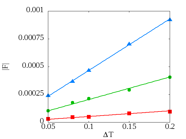
Next, we compare the the numerical results with the obtained $I_{NE}(\omega)$. We use the same values for the diffusion constant $D$, the effective length $L$, and the width $L^{\prime}$ as in the equilibrium system at temperature $T_{\mathrm{ave}}$. Drift force $F$ is estimated from the probability distribution of the interface. Figure. 17 shows that the drift $F$ is proportional to the temperature difference $\Delta T$ as

$$|F|=f(T)\Delta T,$$ (31)

where the constant $f(T)$ is estimated from Fig. 17.

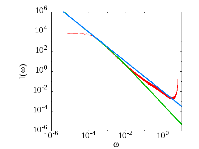
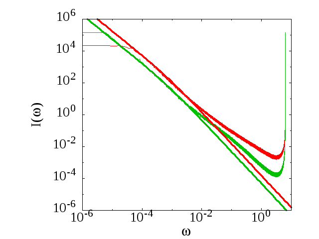
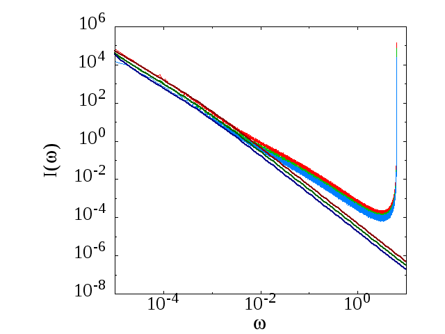
Figure 18 shows the power spectra when $\Delta T$ is very small. We note that the larger the temperature difference $\Delta T$ is, the smaller the magnitude of the power spectrum is and that $I_{NE}(\omega)$ reproduces numerical results in a wide frequency range ($\omega<0.01$). Thus the motion of an interface is considered as normal diffusion with a constant drift to higher temperature region. Addition of the drift term is a nonequilibrium effect. Then, the interface prefers to stay in the high temperature region rather than the center. It causes reduction of the magnitude of the power spectrum for $s_{L_{x}/2}$ in nonequilibrium states. On the other hand, if we consider the position $x_{h}$ defined by $\int_{0}^{x_{h}}P_{st}(x^{\prime})dx^{\prime}=1/2$, the power spectrum of $s_{i}$ takes a maximum value near $i\simeq x_{h}$. Let $x_{h}$ be rounded off to integer $X_{h}$. Figure 19 shows the power spectrum of $s_{Lx/2}$ in equilibrium and nonequilibrium states, and that of $s_{X_{h}}$ in nonequilibrium condition ($\Delta T=0.1$). We see that the power spectrum of $s_{L_{x}/2}$ is larger in equilibrium than in nonequilibrium, but the power spectrum of $s_{X_{h}}$ surpasses the both of them. Figure 20 shows power spectra with various $\Delta T$, which satisfy the scaling form Eq. (30). In higher frequencies, deviation from $I_{NE}(\omega)$ is evident. It is considered to be attributed to the approximation of the interface profile and fluctuations.

VI Summary

In this paper, we have studied interface motion in the two-dimensional Ising model in equilibrium and noneqilibrium situations. To numerically simulate the systems effectively in low temperature, where Creutz dynamics freezes, we have devised the KSC dynamics by combining the Creutz dynamics and KS dynamics. Using the KSC dynamics, we have calculated thermal conductivity with and without an interface and found that the thermal conductivity is larger in the system without an interface than that with an interface. The thermal conductivity is divided into the sum of contributions from Creutz and KS dynamics. Interestingly, the existence of an interface affects the two contributions in an opposite way. When an interface exists, $\kappa_{c}(T)$ is larger and $\kappa_{k}(T)$ is smaller than in the case of no interfaces.

Next, we investigated the probability distribution of the interface position in the KSC dynamics. We have found that the distribution is biased to the higher temperature region and that it is well approximated by an exponential distribution if temperature difference is very small.

In Sec. V, we have analyzed interface dynamics by using the power spectrum of a time sequence of a spin at a site or column averaged magnetization. This is a generalization of the method developed in 3 to two dimensions. In the previous paper 3 , it was shown that the power spectrum of time sequence of a field variable at a position shows the power law behavior with exponent $-3/2$ due to the diffusive motion of the interface. Thus the most straightforward extension to two dimensions is examining the power spectrum of a spin at a fixed site. However, we have seen that in such a spectrum the power law is covered with large-frequency noise and obscure. Although the power spectrum of column averaged magnetization also deviates from the power law, we have revealed that the deviation is largely explained by taking the interface width into account. Moreover, the drift force in nonequilibrium dynamics affects the magnitudes of the power spectrum. Thus, in the two-dimensional Ising model the interface with a width undergoes a diffusive motion with drift force to the higher temperature side in the nonequilibrium situation. Since the position of the interface is related to the magnetization. it may be argued that the power spectrum of magnetization should have enough information for the interface motion. However, the motion of magnetization is purely diffusive and the power spectrum shows only $\omega^{-2}$ behavior. We cannot derive information of interface width from such a spectrum.

The method in 3 and the present paper can be extended to the three-dimensional systems. Because the three-dimensional Ising model has the roughening transition 10 , we may discuss roughening transition through the power spectrum of spin values. It is a future problem.

Appendix A

We start with Eq. (26) with the boundary condition (27). The transition probability is readily obtained as

$$P(x,t|x_{0},0) = \left(\frac{Ke^{-KL}}{\sinh(KL)}\right)^{2}\exp(2K(x+x_{0}))$$ (33)

$$+\sum_{n}\frac{2}{L}\exp(-k_{n}t)\frac{\exp(K(x+x_{0}))e^{-KL}}{\alpha_{n}^{2}+K^{2}}(\alpha_{n}\cos\alpha_{n}x_{0}+K\sin\alpha_{n}x_{0})(\alpha_{n}\cos\alpha_{n}x+K\sin\alpha_{n}x),$$

where $\alpha_{n}$ and $k_{n}$ are defined as

$$\alpha_{n}=\frac{n\pi}{L}\quad(n=1,2,3,.....),$$ (34)

and

$$k_{n}=D(\alpha^{2}_{n}+K^{2})\quad(n=1,2,3,.....).$$ (35)

We use Eq. (19) for the profile of the column-averaged magnetization with an interface of width $L^{\prime}$. Then, the autocorrelation function of $\delta s_{y}(t)=s_{y}(t)-\langle s_{y}\rangle_{st}$ is obtained as

$$\begin{aligned} \lx@intercol\@ADDCLASS{ltx_eqn_lefteqn}$\displaystyle\langle{\delta s_{y}(t)\delta s_{y}(0)}\rangle=$\mbox{}\hfil\lx@intercol\\ &\sum_{n}\left(\frac{2}{L^{2}}\right){\left(\frac{2}{L^{\prime}}\right)}^{2}\frac{e^{2Ky}}{(\alpha_{n}^{2}+K)^{3}}\frac{KL}{\sinh(KL)}\exp(-k_{n}t)\{\frac{1+(-1)^{n+1}\cos({2\alpha_{n}y})}{2}(K\cos(\alpha_{n}\frac{L^{\prime}}{2})\sin(K\frac{L^{\prime}}{2})\\ &+\alpha_{n}\sin(\alpha_{n}\frac{L^{\prime}}{2})\cos(K\frac{L^{\prime}}{2}))^{2}+\frac{1+(-1)^{n}\cos(2\alpha y)}{2}(\alpha_{n}\cos(\alpha_{n}\frac{L^{\prime}}{2})\sin(K\frac{L^{\prime}}{2})-K\sin(\alpha_{n}\frac{L^{\prime}}{2})\cos(K\frac{L^{\prime}}{2}))^{2}\\ &+2\sin(\alpha_{n}y)\cos(\alpha_{n}y)(K\cos(\alpha_{n}\frac{L^{\prime}}{2})\sin(K\frac{L^{\prime}}{2})+\alpha_{n}\sin(\alpha_{n}\frac{L^{\prime}}{2})\cos(K\frac{L^{\prime}}{2}))(\alpha_{n}\cos(\alpha_{n}\frac{L^{\prime}}{2})\sin(K\frac{L^{\prime}}{2})\\ &-K\sin(\alpha_{n}\frac{L^{\prime}}{2})\cos(K\frac{L^{\prime}}{2}))\}\end{aligned}$$ (36)

We put $y=L/2$ and take Fourier transform to obtain the power spectrum

$$\begin{split}I(\omega)&=\sum_{n=1}^{\infty}\frac{2k_{n}}{k_{n}^{2}+\omega^{2}}\frac{1}{L^{2}}\left(\frac{2}{L^{\prime}}\right)^{2}\frac{KL}{\sinh(KL)}\frac{1}{(\alpha_{n}^{2}+K^{2})^{2}}\{\sinh^{2}(K\frac{L^{\prime}}{2})+\sin^{2}(\alpha_{n}\frac{L^{\prime}}{2})\}.\end{split}$$ (37)

When $L$ is large, the sum over $n$ can be replaced by the integral

$$\begin{split}I(\omega)\sim\frac{1}{\pi L}\int_{0}^{\infty}dx\frac{2D}{D^{2}(x^{2}+K^{2})^{2}+\omega^{2}}\frac{KL}{\sinh(KL)}\frac{1}{(x^{2}+K^{2})}\{\sinh^{2}(K\frac{L^{\prime}}{2})+\sin^{2}(\frac{L^{\prime}}{2}x)\}.\end{split}$$ (38)

Using residue calculus, we arrive at

$$I(\omega)\sim \frac{2}{DLL^{\prime 2}}\frac{KL}{\sinh(KL)}\left(\frac{\omega}{D}\right)^{-2}\frac{\sqrt{\sqrt{(K^{2})^{2}+(\frac{\omega}{D})^{2}}+K^{2}}}{\sqrt{(K^{2})^{2}+(\frac{\omega}{D})^{2}}}\left[{-\frac{1}{\sqrt{2}}}\cosh(KL^{\prime})\right.$$ (39)

$$+\exp\left(-L^{\prime}\sqrt{\frac{\sqrt{(K^{2})^{2}+(\frac{\omega}{D})^{2}}-K^{2}}{2}}\right)\left\{\frac{1}{\sqrt{2}}\cos\left(L^{\prime}\sqrt{\frac{\sqrt{(K^{2})^{2}+(\frac{\omega}{D})^{2}}-K^{2}}{2}}\right)\right.$$

$$\left.-\left(\frac{\omega}{D}\right)^{-1}\left(\sqrt{(K^{2})^{2}+(\frac{\omega}{D})^{2}}-K^{2}\right)\sin\left(L^{\prime}\sqrt{\frac{\sqrt{(K^{2})^{2}+(\frac{\omega}{D})^{2}}-K^{2}}{2}}\right)\right\}$$

$$+\left.\left(\frac{\sqrt{\sqrt{(K^{2})^{2}+(\frac{\omega}{D})^{2}}+K^{2}}}{\sqrt{(K^{2})^{2}+(\frac{\omega}{D})^{2}}}\right)^{-1}L^{\prime}\left(\frac{\sinh(KL^{\prime})}{KL^{\prime}}\right)\right].$$