Fast Maximization of Non-Submodular, Monotonic Functions on the Integer Lattice

Abstract

The optimization of submodular functions on the integer lattice has received much attention recently, but the objective functions of many applications are non-submodular. We provide two approximation algorithms for maximizing a non-submodular function on the integer lattice subject to a cardinality constraint; these are the first algorithms for this purpose that have polynomial query complexity. We propose a general framework for influence maximization on the integer lattice that generalizes prior works on this topic, and we demonstrate the efficiency of our algorithms in this context.

1 Introduction

As a natural extension of finite sets $S$ (equivalently, $\{0,1\}^{S}$), optimization of discrete functions on the integer lattice $\mathbb{N}^{S}$ has received attention recently (Alon et al., 2012; Demaine et al., 2014; Soma and Yoshida, 2015). As an example, consider the placement of sensors in a water network (Krause et al., 2008a); in the set version, each sensor takes a value in $\{0,1\}$, which corresponds to whether the sensor was placed. In the lattice version Soma and Yoshida (2015), each sensor has a power level in $\{0,\ldots,b\}\subseteq\mathbb{N}$, to which the sensitivity of the sensor is correlated. As a second example, consider the influence maximization problem (Kempe et al., 2003); instead of the binary seeding of a user, the lattice version enables partial incentives or discounts to be used (Demaine et al., 2014).

Although many results from the optimization of submodular set functions have been generalized to the integer lattice (Soma and Yoshida, 2015, 2016; Ene and Nguyen, 2016), many objective functions arising from applications are not submodular (Bian et al., 2017b; Lin et al., 2017; Das and Kempe, 2011; Horel and Singer, 2016). In this work, we consider maximization subject to a cardinality constraint (MCC), where the function $f$ to be maximized may be non-submodular. Let $k\in\mathbb{N}$ (the budget), $\mathbf{b}\in(\mathbb{N}\cup\{\infty\})^{S}$ (the box), and let $f:\{\mathbf{x}\in\mathbb{N}^{S}:\mathbf{x}\leq\mathbf{b}\}\to\mathbb{R}^{+}$ (the objective) be a non-negative and monotonic function with $f(\mathbf{0})=0$. Then determine

$$\max_{\lVert\mathbf{w}\rVert_{1}\leq k}f(\mathbf{w}),$$ (MCC)

where $\mathbf{w}=(\mathbf{w}_{s})_{s\in S}\in\mathbb{N}^{S}$, $\lVert\mathbf{w}\rVert_{1}=\sum_{s\in S}|\mathbf{w}_{s}|$.

Since the integer lattice may be represented as a multiset of size $k|S|$, one may use results for Problem MCC with non-submodular set functions. In particular, the tight ratio $\frac{1}{\alpha}\left(1-e^{-\alpha\gamma_{s}}\right)$ of the standard greedy algorithm by Bian et al. (2017b), where $\alpha,\gamma_{s}$ are discussed below, applies with the lattice adaptation of the standard greedy algorithm (StandardGreedy) given in Alg. 1. However, this approach requires $\Omega(|S|k)$ queries of $f$, which is not polynomial in the input size $O(|S|\log k)$. Even for applications with set functions, $\Omega(|S|k)$ queries may be prohibitive, and researchers (Leskovec et al., 2007; Mirzasoleiman et al., 2015; Badanidiyuru and Vondrák, 2014) have sought ways to speed up the StandardGreedy algorithm. Unfortunately, these approaches rely upon the submodularity of $f$, and there has been no analogous effort for non-submodular functions.

To quantify the non-submodularity of a lattice function $f$, we generalize the following quantities defined for set functions to the lattice: (1) the diminishing-return (DR) ratio $\gamma_{d}$ of $f$ (Lehmann et al., 2006), (2) the submodularity ratio $\gamma_{s}$ of $f$ (Das and Kempe, 2011), and (3) the generalized curvature $\alpha$ of $f$ (Bian et al., 2017b). Our main contributions are:

• To speed up StandardGreedy (Alg. 1), we adapt the threshold greedy framework of Badanidiyuru and Vondrák (2014) to non-submodular functions; this yields an algorithm (ThresholdGreedy, Alg. 2) with approximation ratio $(1-e^{-\gamma_{d}\gamma_{s}}-\eta)$, for any $\eta>0$, the first approximation algorithm with polynomial query complexity for Problem MCC on the lattice. The query complexity of the StandardGreedy algorithm is improved from $\Omega(nk)$ to $O\left(n\log k\log_{\kappa}\left(\varepsilon^{2}/k\right)\right)$, where $\kappa,\varepsilon\in(0,1)$ are parameters of ThresholdGreedy.

• We introduce the novel approximation algorithm FastGreedy, which combines elements of StandardGreedy and ThresholdGreedy to improve the performance ratio to $(1-e^{-\beta^{*}\gamma_{s}}-\eta)$, where $\beta^{*}$ is at least $\gamma_{d}$ and in many cases is determined by the algorithm. Furthermore, FastGreedy exploits the non-submodularity of the function to decrease its runtime in practice without sacrificing its performance guarantee, while maintaining the same worst-case query complexity as ThresholdGreedy up to a constant factor.

• To demonstrate our algorithms, we introduce a general budget allocation problem for viral marketing, which unifies submodular influence maximization (IM) under the independent cascade model (Kempe et al., 2003) with the non-submodular boosting problem (Lin et al., 2017) and in addition allows partial incentives. We prove a lower bound on the DR and submodularity ratios for this unified framework, and we experimentally validate our proposed algorithms in this setting.

Algorithm 1 StandardGreedy

1:  Input: $f\in\mathcal{F}_{\mathbf{b}}$, $k\in\mathbb{N}$, $\mathbf{b}\in\mathbb{N}^{S}$

2:  Output: $\mathbf{g}\in\mathbb{N}^{S}$

3:  $\mathbf{g}\leftarrow\mathbf{0}$

4:  for $i=1$ to $k$ do

5:     $\mathbf{g}\leftarrow\mathbf{g}+\operatorname*{arg\,max}_{s\in S:\mathbf{g}+\mathbf{s}\leq\mathbf{b}}\delta_{\mathbf{s}}(\mathbf{g})$

6:  return $\mathbf{g}$

2 Related Work

The study of optimization of submodular set functions is too extensive to give a comprehensive overview. On the integer lattice, there have been many efforts to maximize submodular functions, e.g Soma and Yoshida (2017); Bian et al. (2017a); Gottschalk and Peis (2016). To the best of our knowledge, we are the first to study the optimization of non-submodular functions on the integer lattice. In the following discussion, we primarily restrict our attention to the maximization of monotonic, submodular lattice functions subject to a cardinality constraint and the maximization of non-submodular set functions.

Reduction of Ene and Nguyen (2016).

Ene and Nguyen (2016) have given a polynomial-time reduction from the lattice to a set that enables unified translation of submodular optimization strategies to DR-submodular (i.e. DR ratio $\gamma_{d}=1$, see Section 3) functions on the integer lattice. Since this translation is designed for DR-submodular functions, it does not give a polynomial-time algorithm for Problem MCC when $f$ is non-submodular. Specifically, for the case of maximization subject to a cardinality constraint, Ene and Nguyen (2016) rely upon the threshold greedy algorithm for submodular set functions (Badanidiyuru and Vondrák, 2014), which does not work for non-submodular functions without modifications such as the ones in our paper.

Threshold Greedy and Lattice Optimization.

To speed up the StandardGreedy for submodular set functions, Badanidiyuru and Vondrák (2014) introduced the threshold greedy framework, which speeds up the StandardGreedy algorithm for maximizing submodular set functions under cardinality constraint from $O(nk)$ function evaluations to $O\left(\frac{n}{\varepsilon}\log\frac{n}{\varepsilon}\right)$, and it maintains the approximation ratio $(1-1/e-\varepsilon)$, for $\varepsilon>0$. Soma and Yoshida (2016) adapted the threshold approach for efficiently maximizing DR-submodular functions on the integer lattice and provided $(1-1/e-\varepsilon)$-approximation algorithms. Other adaptations of the threshold approach of Badanidiyuru and Vondrák (2014) to the integer lattice include Ene and Nguyen (2016); Soma and Yoshida (2015). To the best of our knowledge, in this work we make the first use of the threshold framework for non-submodular functions.

Our ThresholdGreedy algorithm is an adaptation of the algorithm of Soma and Yoshida (2016) for DR-submodular maximization to non-submodular functions. The non-submodularity requires new analysis, in the following specific ways: (1) during the binary search phase, we cannot guarantee that we find the maximum number of copies whose average gain exceeds the threshold $\tau$; hence, we must settle for any number of copies whose average gain exceeds $\tau$, while ensuring that the gain of adding one additional copy falls belows $\tau$. (2) To prove the performance ratio, we require a combination of the DR ratio $\gamma_{d}$ and the submodularity ratio $\gamma_{s}$. (3) The stopping condition (smallest threshold value) is different resulting from the non-submodularity; the proof this condition is sufficient requires another application of the DR ratio.

Optimization of Non-Submodular Set Functions.

For non-submodular set functions, the submodularity ratio $\gamma_{s}$ was introduced by Das and Kempe (2011); we generalize $\gamma_{s}$ to lattice functions in Section 3, and we show the DR ratio $\gamma_{d}\leq\gamma_{s}$. Bian et al. (2017b) introduced generalized curvature $\alpha$ of a set function, an analogous concept to the DR ratio as we discuss in Section 3. Bian et al. (2017b) extended the analysis of Conforti and Cornuéjols (1984) to non-submodular set functions; together with the submodularity ratio $\gamma_{s}$, they proved StandardGreedy has tight approximation ratio $\frac{1}{\alpha}\left(1-e^{-\gamma_{s}\alpha}\right)$ under cardinality constraint.

The DR ratio $\gamma_{d}$ was introduced by Lehmann et al. (2006) for the valuation functions in the maximum allocation problem for a combinatorial auction; if each valuation function has DR ratio at least $\gamma_{d}$, the maximum allocation problem is a special case of maximizing a set function $f$ with DR ratio $\gamma_{d}$ over a matroid, for which Lehmann et al. (2006) employ the StandardGreedy algorithm (for matroids).

Many other notions of non-submodular set functions have been introduced (Krause et al., 2008b; Horel and Singer, 2016; Borodin et al., 2014; Feige and Izsak, 2013). For a comprehensive discussion of the relation of these and additional notions to the submodularity ratio $\gamma_{s}$, we refer the reader to Bian et al. (2017b).

3 Non-Submodularity on the Lattice

In this section, we define the lattice versions of DR ratio $\gamma_{d}$, submodularity ratio $\gamma_{s}$, and generalized curvature $\alpha$, which are used in the approximation ratios proved in Section 4.

Notations.

For each $s\in S$, let $\mathbf{s}$ be the unit vector with $1$ in the coordinate corresponding to $s$, and 0 elsewhere. We write $\delta_{\mathbf{w}}(\mathbf{v})=f(\mathbf{v}+\mathbf{w})-f(\mathbf{v})$ for $\mathbf{v},\mathbf{w}\in\mathbb{N}^{S}$. Given a box in the integer lattice $\mathbf{b}\in\mathbb{N}^{S}$, let the set of all non-negative, monotonic lattice functions with $f(\mathbf{0})=0$, and domain $\{\mathbf{x}\in\mathbb{N}^{S}:\mathbf{x}\leq\mathbf{b}\}$ be denoted $\mathcal{F}_{\mathbf{b}}$. It is often useful to think of a vector $\mathbf{v}\in\mathbb{N}^{S}$ as a multi-set containing $\mathbf{v}_{s}$ copies of $s\in S$, where $\mathbf{v}_{s}$ is the value of $\mathbf{v}$’s coordinate corresponding to $s$. We use the notation $\{\mathbf{v}\}$ to represent the multiset corresponding to the vector $\mathbf{v}$. Finally, we define $\mathbf{v}\lor\mathbf{w}$ and $\mathbf{v}\land\mathbf{w}$ for $\mathbf{v},\mathbf{w}\in\mathbb{N}^{S}$ to be the vector with the coordinate-wise maximum and minimum respectively. Rather than an algorithm taking an explicit description of the function $f$ as input, we consider the function $f$ as an oracle and measure the complexity of an algorithm in terms of the number of oracle calls or queries.

We begin with the related concepts of DR ratio and generalized curvature.

Definition 1.

Let $f\in\mathcal{F}_{\mathbf{b}}$. The diminishing-return (DR) ratio of $f$, $\gamma_{d}(f)$, is the maximum value in $[0,1]$ such that for any $s\in S$, and for all $\mathbf{v}\leq\mathbf{w}$ such that $\mathbf{w}+\mathbf{s}\leq\mathbf{b}$,

$$\gamma_{d}(f)\delta_{\mathbf{s}}(\mathbf{w})\leq\delta_{\mathbf{s}}(\mathbf{v}).$$

Definition 2.

Let $f\in\mathcal{F}_{\mathbf{b}}$. The generalized curvature of $f$, $\alpha(f)$, is the minimum value in $[0,1]$ such that for any $s\in S$, and for all $\mathbf{v}\leq\mathbf{w}$ such that $\mathbf{w}+\mathbf{s}\leq\mathbf{b}$,

$$\delta_{\mathbf{s}}(\mathbf{w})\geq(1-\alpha(f))\delta_{\mathbf{s}}(\mathbf{v}).$$

The DR ratio extends the notion of DR-submodularity of Soma and Yoshida (2015), which is obtained as the special case $\gamma_{d}=1$. Generalized curvature for set functions was introduced in Bian et al. (2017b). Notice that $\alpha$ results in lower bounds on the marginal gain of $\mathbf{s}$ to a vector $\mathbf{w}$, while $\gamma_{d}$ results in upper bounds on the same quantity:

$$(1-\alpha)\delta_{\mathbf{s}}(\mathbf{v})\leq\delta_{\mathbf{s}}(\mathbf{w})\leq\frac{1}{\gamma_{d}}\delta_{\mathbf{s}}(\mathbf{v}),$$

whenever $\mathbf{v}\leq\mathbf{w}$ and the above expressions are defined. Next, we generalize the submodularity ratio of Das and Kempe (2011) to the integer lattice.

Definition 3.

Let $f\in\mathcal{F}_{\mathbf{b}}$. The submodularity ratio of $f$, $\gamma_{s}(f)$, is the maximum value in $[0,1]$ such that for all $\mathbf{v},\mathbf{w}$, such that $\mathbf{v}\leq\mathbf{w}$,

$$\gamma_{s}(f)(f(\mathbf{w})-f(\mathbf{v}))\leq\sum_{s\in\{\mathbf{w}-\mathbf{v}\}}\delta_{\mathbf{s}}(\mathbf{v}).$$

The next proposition, proved in Appendix C, shows the relationship between DR ratio and submodularity ratio.

Proposition 1.

For all $f\in\mathcal{F}_{\mathbf{b}}$, $\gamma_{d}(f)\leq\gamma_{s}(f)$.

In the rest of this work, we will parameterize functions by the non-submodularity ratios defined above and partition functions into the sets $\mathcal{F}_{\mathbf{b}}^{\gamma_{d},\gamma_{s},\alpha}=\{f\in\mathcal{F}_{\mathbf{b}}:\gamma_{d}(f)=\gamma_{d},\gamma_{s}(f)=\gamma_{s},\alpha(f)=\alpha\}$.

Greedy versions.

In the proofs of this paper, the full power of the parameters defined above is not required. It suffices to consider restricted versions, where the maximization is taken over only those vectors which appear in the ratio proofs. We define these greedy versions in Appendix B and include more discussion in Remark 1 of Section 4.1.

4 Algorithms

4.1 The ThresholdGreedy Algorithm

In this section, we present the algorithm ThresholdGreedy (Alg. 2) to approximate Problem MCC with ratio $1-e^{-\gamma_{g}\gamma_{s}}-\eta$ with polynomial query complexity. Appendix D contains the proofs of all lemmas, claims, and omitted details from this section.

Description.

ThresholdGreedy operates by considering decreasing thresholds for the marginal gain in its outer for loop; for each threshold $\tau$, the algorithm adds on line 7 elements whose marginal gain exceeds $\tau$ as described below. The parameter $\kappa\in(0,1)$ determines the stepsize between successive thresholds; the algorithm continues until the budget $k$ is met (line 8) or the threshold is below a minimum value dependent on the parameter $\varepsilon\in(0,1)$.

Intuitively, the goal of the threshold approach (Badanidiyuru and Vondrák, 2014) for submodular set functions is as follows. At each threshold (i.e., iteration of the outer for loop), add all elements whose marginal gain exceeds $\tau$ to the solution $\mathbf{g}$. On the lattice, adding all copies of $s\in S$ whose average gain exceeds $\tau$ on line 7 would require the addition of the maximum multiple $l\mathbf{s}$ such that the average marginal gain exceeds $\tau$:

$$\delta_{l\mathbf{s}}(\mathbf{g})\geq l\tau,$$ (P1)

as in the threshold algorithm of Soma and Yoshida (2016) for DR-submodular functions, in which the maximum $l$ is identified by binary search. However, since $f$ is not DR-submodular, it is not always the case that $\delta_{\mathbf{s}}(\mathbf{g}+l\mathbf{s})\geq\delta_{\mathbf{s}}(\mathbf{g}+(l+1)\mathbf{s})$, for each $l$. For this reason, we cannot find the maximum such $l$ by binary search. Furthermore, even if we found the maximum $l$ for each $s\in S$, we could not guarantee that all elements of marginal gain at least $\tau$ were added due to the non-submodularity of $f$: an element whose gain is less than $\tau$ when considered in the inner for loop might have gain greater than $\tau$ after additional elements are added to the solution.

ThresholdGreedy more conservatively ensures that the number $l$ chosen for each $s\in S$ satisfies both (P1) and

$$\delta_{\mathbf{s}}(\mathbf{g}+l\mathbf{s})<\tau,$$ (P2)

but it is not necessarily the maximum such $l$.

Pivot.

Any $l$ satisfying both (P1) and (P2) is termed a pivot with respect to $\mathbf{g},s,\tau$. Perhaps surprisingly, a valid pivot can be found with binary search in $O(\log\mathbf{b}_{max})=O(\log k)$ function queries, where $\mathbf{b}_{max}=\max_{s\in S}\mathbf{b}_{s}$; discussion of BinarySearchPivot and proof of this results is provided in Appendix D, Lemma 2. By finding a pivot for each $s\in S$, ThresholdGreedy does not attempt to add all elements exceeding the marginal gain of threshold $\tau$; instead, ThresholdGreedy maintains the following property at each threshold.

Property 1.

Let $\mathbf{g}_{\tau}$ be the solution of ThresholdGreedy immediately after the iteration of the outer for loop corresponding to threshold $\tau$. Then for each $s\in S$, there exists $\mathbf{h}\leq\mathbf{g}_{\tau}$ such that $\delta_{\mathbf{s}}(\mathbf{h})<\tau$.

Algorithm 2 ThresholdGreedy

1:  Input: $f\in\mathcal{F}_{\mathbf{b}}$, $k\in\mathbb{N}$, $\kappa,\varepsilon\in(0,1)$.

2:  Output: $\mathbf{g}\in\mathbb{N}^{S}$

3:  $\mathbf{g}\leftarrow\mathbf{0}$, $M\leftarrow\max_{s\in S}f(\mathbf{s})$.

4:  for $\left(\tau=M;\tau\geq\frac{\kappa\varepsilon^{2}M}{k};\tau\leftarrow\kappa\tau\right)$ do

5:     for $s\in S$ do

6:        $l\leftarrow$BinarySearchPivot$(f,\mathbf{g},\mathbf{b},s,k,\tau)$

7:        $\mathbf{g}\leftarrow\mathbf{g}+l\mathbf{s}$

8:        if $\lVert\mathbf{g}\rVert_{1}=k$ then

9:           return $\mathbf{g}$

10:  return $\mathbf{g}$

Performance ratios.

Next, we present the main result of this section, the performance guarantee involving the DR and submodularity ratios. Observe that the query complexity of ThresholdGreedy is polynomial in the input size $O(n\log k)$.

Theorem 1.

Let an instance of Problem MCC be given, with $f\in\mathcal{F}_{\mathbf{b}}^{\gamma_{d},\gamma_{s},\alpha}$. If $\mathbf{g}$ is the solution returned by ThresholdGreedy and $\mathbf{\Omega}$ is an optimal solution to this instance, then

$$f(\mathbf{g}) \geq\left(1-e^{-\kappa\gamma_{d}\gamma_{s}}-\varepsilon\right)f(\mathbf{\Omega}).$$

The query complexity of ThresholdGreedy is $O\left(n\log k\log_{\kappa}\left(\varepsilon^{2}/k\right)\right)$.

If $\eta>0$ is given, the assignment $\kappa=(1-\eta/2)$, $\varepsilon=\eta/2$ yields performance ratio at least $1-e^{-\gamma_{d}\gamma_{s}}-\eta$.

Proof.

If $\gamma_{d}<\varepsilon$, the ratio holds trivially; so assume $\gamma_{d}\geq\varepsilon$. The proof of the following claim requires an application of the DR ratio.

Claim 1.

Let $\mathbf{g}$ be produced by a modified version of ThresholdGreedy that continues until $\lVert\mathbf{g}\rVert_{1}=k$. If we show $f(\mathbf{g})\geq(1-e^{-\kappa\gamma_{d}\gamma_{s}})f(\mathbf{\Omega})$, the results follows.

Thus, for the rest of the proof let $\mathbf{g}$ be as described in Claim 1. Let $\mathbf{g}^{t}$ be the value of $\mathbf{g}$ after the $t$th execution of line 7 of ThresholdGreedy. Let $l^{t}$ be the $t$th pivot, such that $\mathbf{g}^{t}=\mathbf{g}^{t-1}+l^{t}\mathbf{s}^{t}$. The next claim lower bounds the marginal gain in terms of the DR ratio and the previous threshold.

Claim 2.

For each $s\in\{\mathbf{\Omega}-\mathbf{g}^{t-1}\wedge\mathbf{\Omega}\}$,

$$l^{t}\gamma_{d}\kappa\delta_{\mathbf{s}}(\mathbf{g}^{t-1})\leq f(\mathbf{g}^{t})-f(\mathbf{g}^{t-1}).$$

Proof.

Let $\tau$ be the threshold at which $l^{t}\mathbf{s}^{t}$ is added to $\mathbf{g}^{t-1}$; let $s\in\{\mathbf{\Omega}-\mathbf{g}^{t-1}\wedge\mathbf{\Omega}\}$. If $\tau$ is the first threshold,

$$\gamma_{d}\delta_{\mathbf{s}}(\mathbf{g}^{t-1})\leq\delta_{\mathbf{s}}(\mathbf{0})\leq\tau<\frac{\tau}{\kappa}.$$

If $\tau$ is not the first threshold, $\tau^{\prime}=\tau/\kappa$ is the previous threshold value of the previous iteration of the outer for loop. By Property 1, there exists $\mathbf{h}\leq\mathbf{g}_{\tau^{\prime}}\leq\mathbf{g}^{t-1}$, such that $\delta_{\mathbf{s}}(\mathbf{h})<\tau^{\prime}$. By the definition of DR ratio, $\gamma_{d}\delta_{\mathbf{s}}(\mathbf{g}^{t-1})\leq\delta_{\mathbf{s}}(\mathbf{h})<\tau^{\prime}=\tau/\kappa$.

In either case, by the fact that property (P1) of a pivot holds for $l^{t}$, we have

$$f(\mathbf{g}^{t})-f(\mathbf{g}^{t-1})\geq l^{t}\tau\geq l^{t}\gamma_{d}\kappa\delta_{\mathbf{s}}(\mathbf{g}^{t-1}).\qed$$

Since $|\mathbf{\Omega}|\leq k$, we have by Claim 2

$$f(\mathbf{g}^{t})-f(\mathbf{g}^{t-1}) \geq\frac{l^{t}\gamma_{d}\kappa}{k}\sum_{s\in\left\{\mathbf{\Omega}-(\mathbf{g}^{t-1}\wedge\mathbf{\Omega})\right\}}\delta_{\mathbf{s}}(\mathbf{g}^{t-1})$$

$$=\frac{l^{t}\gamma_{d}\kappa}{k}\sum_{s\in\left\{\mathbf{\Omega}\vee\mathbf{g}^{t-1}-\mathbf{g}^{t-1}\right\}}\delta_{\mathbf{s}}(\mathbf{g}^{t-1})$$

$$\geq\frac{l^{t}\gamma_{d}\gamma_{s}\kappa}{k}\left(f(\mathbf{\Omega}\vee\mathbf{g}^{t-1})-f(\mathbf{g}^{t-1})\right)$$

$$\geq\frac{l^{t}\gamma_{d}\gamma_{s}\kappa}{k}\left(f(\mathbf{\Omega})-f(\mathbf{g}^{t-1})\right),$$

where the equality follows from the lattice identity $\mathbf{v}\vee\mathbf{w}-\mathbf{v}=\mathbf{w}-\mathbf{v}\wedge\mathbf{w}$ for all $\mathbf{v},\mathbf{w}\in\mathbb{N}^{S}$, the second inequality is by definition of the submodularity ratio, and the third inequality is from monotonicity. From here, we obtain $f(\mathbf{g})\geq\left(1-\prod_{t=1}^{T}\left(1-\frac{l^{t}\gamma_{d}\gamma_{s}\kappa}{k}\right)\right)f(\mathbf{\Omega}),$ from which the hypothesis of Claim 1 follows.

Query complexity.

The for loop on line 4 (Alg. 2) iterates at most $\log_{\kappa}\varepsilon^{2}/k$ times; each iteration requires $O(n\log k)$ queries, by Lemma 2. ∎ For additional speedup, the inner for loop of FastGreedy may be parallelized, which divides the factor of $n$ in the query complexity by the number of threads but worsens the performance ratio; in addition to $\gamma_{d},\gamma_{s}$, the generalized curvature $\alpha$ is required in the proof.

Corollary 1.

If the inner for loop of ThresholdGreedy is parallelized, the performance ratio becomes $1-e^{-(1-\alpha)\gamma_{d}\gamma_{s}}-\eta$, for $\eta>0$.

Remark 1.

A careful analysis of the usage of $\gamma_{d}$,$\gamma_{s}$ in the proof of Theorem 1 shows that the full power of the definitions of these quantities is not required. Rather, it is sufficient to consider ThresholdGreedy versions of these parameters, as defined in Appendix B. In the same way, we also have FastGreedy version of $\gamma_{s}$ based upon the proof of Theorem 2. The FastGreedy version of the DR ratio is an integral part of how the algorithm works and is calculated directly by the algorithm, as we discuss in the next section.

4.2 The FastGreedy Algorithm

The proof of the performance ratio of ThresholdGreedy requires both the submodularty ratio $\gamma_{s}$ and the DR ratio $\gamma_{d}$. In this section, we provide an algorithm (FastGreedy, Alg. 3) that achieves ratio $1-e^{-\beta^{*}\gamma_{s}}-\eta$, with factor $\beta^{*}\geq\gamma_{d}$ that it can determine during its execution. Appendix E provides proofs for all lemmas, claims, and omitted details.

Description.

FastGreedy employs a threshold framework analogous to ThresholdGreedy. Each iteration of the outer while loop of FastGreedy is analogous to an iteration of the outer for loop in ThresholdGreedy, in which elements are added whose marginal gain exceeds a threshold. FastGreedy employs BinarySearchPivot to find pivots for each $s\in S$ for each threshold value $\tau$. Finally, the parameter $\varepsilon$ determines a minimum threshold value.

As its threshold, FastGreedy uses $\tau=\beta\kappa m$, where $m$ is the maximum marginal gain found on line 5, parameter $\kappa$ is the intended stepsize between thresholds as in ThresholdGreedy, and $\beta$ is an upper bound on the DR ratio $\gamma_{d}$, as described below. This choice of $\tau$ has the following advantages over the approach of ThresholdGreedy: (1) since the threshold is related to the maximum marginal gain $m$, the theoretical performance ratio is improved; (2) the use of $\beta$ to lower the threshold ensures the same worst-case query complexity as ThresholdGreedy and leads to substantial reduction of the number of queries in practice, as we demonstrate in Section 6.

FastGreedy DR ratio $\beta^{*}$.

If FastGreedy is modified to continue until $\lVert\mathbf{g}\rVert_{1}=k$, let the final, smallest value $\beta^{*}$ of $\beta$ be termed the FastGreedy DR ratio on the instance. The FastGreedy DR ratio $\beta^{*}$ is at least the DR ratio $\gamma_{d}$ of the function, up to the parameter $\delta$:

Lemma 1.

Let parameters $\kappa,\delta,\varepsilon\in(0,1)$ be given. Throughout the execution of FastGreedy on an instance of Problem MCC with $f\in\mathcal{F}^{\gamma_{d},\gamma_{s}}_{\mathbf{b}}$, $\beta\geq\gamma_{d}\delta$. Since $\varepsilon$ can be arbitrarily small, $\beta^{*}\geq\gamma_{d}\delta$.

Proof.

Initally, $\beta=1$; it decreases by a factor of $\delta\in(0,1)$ at most once per iteration of the while loop. Suppose $\beta\leq\gamma_{d}$ for some iteration $i$ of the while loop, and let $\mathbf{g}$ have the value assigned immediately after iteration $i$, $m$ have the value assigned after line 5 of iteration $i$. Since a valid pivot was found for each $s\in S$ during iteration $i$, by property (P2) there exists $\mathbf{g}^{s}\leq\mathbf{g}$, $\delta_{\mathbf{s}}(\mathbf{g}^{s})<\beta\kappa m\leq\gamma_{d}\kappa m$. Hence $\delta_{\mathbf{s}}(\mathbf{g})\leq\kappa m$, by the definition of DR ratio. In iteration $i+1$, $m^{\prime}$ has the value of $m$ from iteration $i$, so the value of $m$ computed during iteration $i+1$ is at most $\kappa m^{\prime}$, and $\beta$ does not decrease during iteration $i+1$. ∎

Algorithm 3 FastGreedy

1:  Input: $f\in\mathcal{F}_{\mathbf{b}}$, $k\in\mathbb{N}$, $\kappa,\delta,\varepsilon\in(0,1)$.

2:  Output: $\mathbf{g}\in\mathbb{N}^{S}$

3:  $\mathbf{g}\leftarrow 0$, $M\leftarrow\max_{s\in S}f(\mathbf{s})$, $m\leftarrow M,m^{\prime}\leftarrow M/\kappa$, $\beta\leftarrow 1$

4:  while $m\geq M\varepsilon^{2}/k$ do

5:     $m\leftarrow\max_{s\in S}\delta_{\mathbf{s}}(\mathbf{g})$

6:     if $m>\kappa m^{\prime}$ then

7:        $\beta\leftarrow\beta\delta$

8:     $m^{\prime}\leftarrow m$

9:     $\tau\leftarrow\beta\kappa m$

10:     for $s\in S$ do

11:        $l\leftarrow$BinarySearchPivot$(f,\mathbf{g},\mathbf{b},s,k,\tau)$

12:        $\mathbf{g}\leftarrow\mathbf{g}+l\mathbf{s}$

13:        if $\lVert\mathbf{g}\rVert_{1}=k$ then

14:           return $\mathbf{g}$

15:  return $\mathbf{g}$

Performance ratio.

Next, we present the main result of this section. In contrast to ThresholdGreedy, the factor of $\gamma_{d}$ in the performance ratio has been replaced with $\beta^{*}$; at the termination of the algorithm, the value of $\beta^{*}$ is an output of FastGreedy if the solution $\mathbf{g}$ satisfies $\lVert\mathbf{g}\rVert_{1}=k$. In any case, by Lemma 1, the performance ratio is at worst the same as that of ThresholdGreedy.

Theorem 2.

Let an instance of Problem MCC be given, with $f\in\mathcal{F}_{\mathbf{b}}^{\gamma_{d},\gamma_{s}}$. Let $\mathbf{g}$ be the solution returned by FastGreedy with parameters $\kappa,\delta,\varepsilon\in(0,1)$, and let $\mathbf{\Omega}$ be an optimal solution to this instance; also, suppose $\gamma_{d}\geq\varepsilon$. Let $\beta^{*}$ be the FastGreedy DR ratio on this instance. Then,

$$f(\mathbf{g}) \geq\left(1-e^{-\kappa\beta^{*}\gamma_{s}}-\varepsilon\right)f(\mathbf{\Omega})$$

The worst-case query complexity of FastGreedy is $O\left(\left(\log_{\delta}(\gamma_{d})\log_{\kappa}(\gamma_{d})+\log_{\kappa}\varepsilon^{2}/k\right)n\log k\right).$

If $\eta>0$ is given, the assignment $\kappa=(1-\eta/2)$, $\varepsilon=\eta/2$ yields performance ratio at least $1-e^{-\beta^{*}\gamma_{s}}-\eta$.

Proof of query complexity.

The performance ratio is proved in Appendix E. Let $m^{\prime}_{1},\ldots,m^{\prime}_{K}$ be the sequence of $m^{\prime}$ values in the order considered by the algorithm. By Lemma 1, $m^{\prime}_{j}>\kappa m^{\prime}_{j-1}$ at most $\Gamma=\log_{\delta}\gamma_{d}$ times; label each such index $j$ an uptick, and let $j_{1},\ldots,j_{l}$ be the indices of each uptick in order of their appearance. Also, let $k_{i}$ be the first index after $j_{i}$ such that $m^{\prime}_{k_{i}}\leq\kappa m^{\prime}_{j_{i}-1}$, for each $i\in\{1,\ldots,l\}$.

Next, we will iteratively delete from the sequence of $m^{\prime}$ values. Initially, let $\ell=l$ be the last uptick in the sequence; delete all terms $m^{\prime}_{j_{\ell}},\ldots,m^{\prime}_{k_{\ell}-1}$ from the $m^{\prime}$ sequence. Set $\ell=\ell-1$ and repeat this process until $\ell=0$.

Claim 3.

For each $\ell$ selected in the iterative deletion above, there are at most $\log_{\kappa}\gamma_{d}$ values deleted from the sequence.

By Claim 3 and the bound on the number of upticks, we have deleted at most $\log_{\kappa}\gamma_{d}\log_{\delta}\gamma_{d}$ thresholds $m^{\prime}$ from the sequence; every term in the remaining sequence satisfies $m^{\prime}_{j}\leq\kappa m^{\prime}_{j-1}$; hence, the remaining sequence contains at most $\log_{\kappa}\varepsilon^{2}/k$ terms, by its initial and terminal values. The query complexity follows from the number of queries per value of $m^{\prime}$, which is $O(n\log k)$ by Lemma 2. ∎

5 Influence Maximization: A General Framework

In this section, we provide a non-submodular framework for viral marketing on a social network that unifies the classical influence maximization (Kempe et al., 2003) with the boosting problem (Lin et al., 2017).

Overview.

The goal of influence maximization is to select seed users (i.e. initially activated users) to maximize the expected adoption in the social network, where the total number of seeds is restricted by a budget, such that the expected adoption in the social network is maximized. The boosting problem is, given a fixed seed set $S$, to incentivize (i.e. increase the susceptibility of a user to the influence of his friends) users within a budget such that the expected adoption with seed set $S$ increases the most.

Our framework combines the above two scenarios with a partial incentive: an incentive (say, $x$% off the purchase price) increases the probability a user will purchase the product independently and increases the susceptibility of the user to the influence of his friends. Hence, our problem asks how to best allocate the budget between (partially) seeding users and boosting the influence of likely extant seeds. Both the classical influence maximization and the non-submodular boosting problem can be obtained as special cases, as shown in Appendix F.

Our model is related to the formulation of Demaine et al. (2014); however, they employ a submodular threshold-based model, while our model is inherently non-submodular due to the boosting mechanism (Lin et al., 2017). Also, GIM is related to the submodular budgeted allocation problem of Alon et al. (2012), in which the influence of an advertiser increases with the amount of budget allocated; the main difference with GIM is that we modify incoming edge weights with incentives instead of outgoing, which creates the boosting mechanism responsible for the non-submodularity.

Model.

Given a social network $G=(V,E)$, and a product $p$, we define the following model of adoption. The allocation of budget to $u$ is thought of as a discount towards purchasing the product; this discount increases the probability that this user will adopt or purchase the product. Furthermore, this discount increases the susceptibility of the user to influence from its (incoming) social connections.

Formally, an incentive level $\mathbf{x}_{u}$ is chosen for each user $u$. With independent probability $p(u,\mathbf{x}_{u})$, user $u$ initially activates or adopts the product; altogether, this creates a probabilistic initial set $S$ of activated users. Next, through the classical Independent Cascade (IC) model of adoption, users influence their neighbors in the social network; wherein the weight $p(v,u,\mathbf{x}_{u})$ for edge $(v,u)$ is determined by the incentive level $\mathbf{x}_{u}$ of user $u$ as well as the strength of the social connection from $v$ to $u$.

We write $p^{\mathbf{x}}(H,T)$ to denote the probability of full graph realization $H$ and seed set $T$ when $\mathbf{x}$ gives the incentive levels for each user. We write $R(H,T)$ to denote the size of the reachable set from $T$ in realization $H$. The expected activation in the network given a choice $\mathbf{x}$ of incentive levels is given by $\mathbb{I}(\mathbf{x})=\sum_{T\subseteq V}\sum_{H\subseteq G}p^{\mathbf{x}}(H,T)R(H,T),$ where an explicit formula for $p^{\mathbf{x}}(H,T)$ is given in Appendix F. Finally, let $\mathbb{A}(\mathbf{x})=\mathbb{I}(\mathbf{x})-\mathbb{I}(\mathbf{0})$.

Definition 4 (Generalized Influence Maximization (GIM)).

Let social network $G=(V,E)$ be given, together with the mappings $i\mapsto p(u,i)$, $i\mapsto p(u,v,i)$, for all $u\in V,(u,v)\in E$, for each $i\in\{0,\ldots,L\}$, where $L$ is the number of incentive levels. Given budget $k$, determine incentive levels $\mathbf{x}$, with $\lVert\mathbf{x}\rVert_{1}\leq k$, such that $\mathbb{A}(\mathbf{x})$ is maximized.

Bound on non-submodularity.

Next, we provide a lower bound on the greedy submodularity ratios (see Appendix B). We emphasize that the assumption that the probability mappings as a function of incentive level be submodular does not imply the objective $\mathbb{A}(\mathbf{x})$ is DR-submodular. Theorem 3 is proved in Appendix F.

Theorem 3.

Let $\mathcal{I}$ be an instance of GIM, with budget $k$. Let ${c_{e}}=\max_{(u,v)\in E,i\in L}\frac{p(u,v,i+1)}{p(u,v,i)}$, $c_{n}=\max_{x\in V,i\in L}\frac{p(x,i+1)}{p(x,i)}$. Suppose for all $(u,v)\in E,w\in V$, the mappings $i\mapsto p(u,v,i)$, $i\mapsto p(w,i)$ are submodular set functions. Then, the greedy submodularity ratios defined in Appendix B and the FastGreedy DR ratio are lower bounded by $c_{e}^{-k\Delta}c_{n}^{-k},$ where $\Delta$ is the maximum in-degree in $G$.

6 Experimental Evaluation

In this section, we evaluate our proposed algorithms for the GIM problem defined in Section 5. We evaluate our algorithms as compared with StandardGreedy; by the naive reduction of the lattice to sets in exponential time, this algorithm is equivalent performing this reduction and running the standard greedy for sets, the performance of which for non-submodular set functions was analyzed by Bian et al. (2017b).

In Section 6.1, we describe our methodology; in Section 6.2, we compare the algorithms and non-submodularity parameters. In Appendix G.1, we explore the behavior of FastGreedy as the parameters $\delta,\kappa$, and $\varepsilon$ are varied.

6.1 Methodology

Our implementation uses Monte Carlo sampling to estimate the objective value $\mathbb{A}(\mathbf{x})$, with $10\,000$ samples used. As a result, each function query is relatively expensive.

We evaluate on two networks taken from the SNAP dataset Leskovec and Krevl (2014): ca-GrQc (“GrQc”; 15k nodes, 14.5K edges) and facebook (“Facebook”; 4k nodes, 176K edges). Unless otherwise specified, we use 10 repetitions per datapoint and display the mean. The width of shaded intervals is one standard deviation. Standard greedy is omitted from some figures where running time is prohibitive. Unless noted otherwise, we use default settings of $\varepsilon=0.05$, $\delta=0.9$, $\kappa=0.95$. We use a uniform box constraint and assign each user the same number of incentive levels; the maximum incentive level for a user corresponds to giving the product to the user for free and hence deterministically seeds the user; we adopt linear models for the mappings $i\mapsto p(u,i)$, $i\mapsto p(u,v,i)$. We often plot versus $K$, which is defined as the maximum number of deterministic seeds; for example, if $k=200$ with $10$ incentive levels, then $K=20$.

6.2 Results

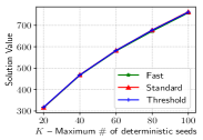
(a) GrQc (10 levels)

(b) Facebook (100 levels)

Figure 1: Activation $\mathbb{A}(\mathbf{g})$ for the solution returned by each algorithm.

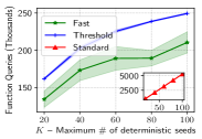
(a) GrQc (10 levels)

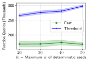
(b) Facebook (100 levels)

Figure 2: Total function queries on the GrQc and Facebook networks.

(a) GrQc (10 levels)

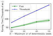
(b) Facebook (100 levels)

Figure 3: Runtime on the GrQc and Facebook networks with 100 levels.

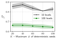
(a) GrQc

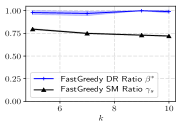
(b) BA network

Figure 4: (a): The value of FastGreedy DR ratio $\beta^{*}$ on the GrQc dataset. (b): FastGreedy submodularity ratio $\gamma_{s}$ and FastGreedy DR Ratio $\beta^{*}$ on a small, random BA network.

In this section, we demonstrate the following: (1) our algorithms exhibit virtually identical quality of solution with StandardGreedy, (2) our algorithms query the function much fewer times, which leads to dramatic runtime improvement over StandardGreedy, (3) FastGreedy further reduces the number of queries of ThresholdGreedy while sacrificing little in solution quality, and (4) the non-submodularity parameters on a small instance are computed, which provides evidence that our theoretical performance ratios are useful.

Quality of Solution

In Fig. 1(a), we plot $\mathbb{A}(\mathbf{g})$ for the solution returned by each algorithm on the GrQc network with $10$ incentive levels; the difference in quality of solution returned by the three algorithms is negligible. In Fig. 1(b), we plot the same for the Facebook network with $100$ incentive levels; on Facebook, we drop StandardGreedy due to its prohibitive runtime. FastGreedy is observed to lose a small (up to 3%) factor, which we consider acceptable in light of its large runtime improvement, which we discuss next.

Number of Queries

Next, we present in Fig. 2 the number of function queries each algorithm requires on the GrQc and Facebook networks. StandardGreedy required up to 20M queries on Facebook, hence it is not shown in Fig. 2(b). Both of our algorithms provide a large improvement over StandardGreedy; in particular, notice that StandardGreedy increases linearly with $k$, while both of the others exhibit logarithmic increase in agreement with the theoretical query complexity of each. Furthermore, FastGreedy uses at least 14.5% fewer function queries than ThresholdGreedy and up to 43% fewer as $k$ grows.

In terms of CPU runtime, we show in Fig. 3 that FastGreedy significantly outperforms ThresholdGreedy; hence, the runtime appears to be dominated by the number of function queries as expected.

Non-Submodularity Parameters

The value of the FastGreedy DR ratio $\beta^{*}$ on GrQc is shown in Fig. 4(a); notice that it is relatively stable as the budget increases from $K=20$ to $100$, although there is substantial drop from $10$ incentive levels to $100$; this may be explained as an increase in the non-submodularity resulting from inaccurate sampling of $\mathbb{A}$, since it is more difficult to detect differences between the finer levels. Still, on all instances tested, $\beta^{*}>0.6$, which suggests the worst-case performance ratio of FastGreedy is not far from that of StandardGreedy.

Finally, we examine the various non-submodularity parameters on a very small instance which admits their computation: a random Barabasi-Albert network with $10$ nodes and $10$ incentive levels. We compute the FastGreedy version of the submodularity ratio $\gamma_{s}$ defined in Appendix B by direct enumeration and consider the FastGreedy DR ratio $\beta^{*}$. Results are shown in Fig. 4(b). The value of $\beta^{*}$ is close to $1$ and remains constant with increasing budget $k$, while the FastGreedy submodularity ratio decreases slowly with $k$. With $\beta^{*}$ and the FastGreedy $\gamma_{s}$, we can compute the worst-case performance ratio of FastGreedy across these instances: $0.449692$.

7 Conclusions

In this work, we provide two approximation algorithms for maximizing non-submodular functions with respect to a cardinality constraint on the integer lattice with polynomial query complexity. Since set functions are a special case, our work provides faster algorithms for the same problem with set functions than the standard greedy algorithm, although the performance ratio degrades from at least $1-e^{-\gamma_{s}}$ to $1-e^{-\beta^{*}\gamma_{s}}$, where $\beta^{*}$ is the FastGreedy DR Ratio. We propose a natural application of non-submodular influence maximization, for which we lower bound the relevant non-submodularity parameters and validate our algorithms.

Appendix A Organization of the Appendix

Appendix B defines the greedy versions of the non-submodularity parameters.

Appendix C provides omitted proofs from Section 3.

Appendix D defines the BinarySearchPivot procedure and omitted proofs from Section 4.1.

Appendix E provides omitted proofs from Section 4.2.

Appendix F defines the Independent Cascade model, proves that classical IM and boosting are subproblems of our IM model, and provides the proof of Theorem 3 from Section 5.

Appendix G provides additional experimental results characterizing the parameters of FastGreedy.

Appendix H presents details of our GIM implementation.

Appendix B Greedy Versions of Non-Submodularity Parameters

We define various greedy versions of the non-submodularity parameters in this section. In this work, these are referred to as FastGreedy submodularity ratio, etc., where the instance is clear from the context.

ThresholdGreedy DR ratio.

Definition 5 (ThresholdGreedy DR ratio).

Let an instance $\mathcal{I}$ of Problem MCC be given, with budget constraint $k$. Let $\mathbf{g}^{1},\ldots,\mathbf{g}^{T}$ be the sequence of values $\mathbf{g}$ takes during execution of ThresholdGreedy on $\mathcal{I}$. The ThresholdGreedy version of the DR ratio on $\mathcal{I}$ $\gamma_{d}^{\text{TG},\mathcal{I}}(f)\in[0,1]$, is the maximum value such that for any $i\in\{1,\ldots,T\}$, for any $s\in S$, if $\mathbf{g}^{i,s}$ is the value of the greedy vector immediately after $s$ was considered during the inner for loop of the threshold directly preceding the one in which $\mathbf{g}^{i}$ was considered ($\mathbf{g}^{i,s}=\mathbf{0}$ if $\mathbf{g}^{i}$ was considered during the first threshold),

$$\gamma_{d}^{\text{TG},\mathcal{I}}\delta_{\mathbf{s}}(\mathbf{g}^{i})\leq\delta_{\mathbf{s}}(\mathbf{g}^{i,s}).$$

Greedy versions of submodularity ratio.

Definition 6.

Let $\mathcal{A}\in\{\text{StandardGreedy},\text{ThresholdGreedy}\}$, and let an instance $\mathcal{I}$ of Problem MCC be given, with budget constraint $k$. Let $\mathbf{g}^{1},\ldots,\mathbf{g}^{T}$ be the sequence of values $\mathbf{g}$ takes during execution of $\mathcal{A}$ on $\mathcal{I}$. The $\mathcal{A}$ version of the submodularity ratio on $\mathcal{I}$ $\gamma_{s}^{\mathcal{A},\mathcal{I}}\in[0,1]$, is the maximum value such that for any $s\in S$, for any $i\in\{1,\ldots,T\}$, for any $\mathbf{w}$ such that $\mathbf{g}^{i}\leq\mathbf{w}$ and $\lVert\mathbf{w}-\mathbf{g}^{i}\rVert_{1}\leq k$ and $\mathbf{w}\leq\mathbf{b}$,

$$\gamma_{s}^{\mathcal{A},\mathcal{I}}\left[f(\mathbf{w})-f(\mathbf{g}^{i})\right]\leq\sum_{s\in\{\mathbf{w}-\mathbf{g}^{i}\}}\delta_{\mathbf{s}}(\mathbf{g}^{i}).$$

The FastGreedy submodularity ratio differs from the above two only in that the sequence of vectors $\mathbf{g}^{1},\ldots,\mathbf{g}^{T}$ are the value of the greedy vector $\mathbf{g}$ at the beginning of each iteration of the outer while loop, instead of all values of $\mathbf{g}$ during execution of the algorithm.

Appendix C Proofs for Section 3

Proof of Proposition 1.

Suppose $\mathbf{v}\leq\mathbf{w}\in\mathbb{N}^{S}$. Let $\{\mathbf{w}-\mathbf{v}\}=\{s_{1},...,s_{l}\}$. Then,

$$\gamma_{d}(f(\mathbf{w})-f(\mathbf{v})) =\gamma_{d}\sum_{i=1}^{l}[f(\mathbf{v}+\mathbf{s}_{1}+...+\mathbf{s}_{i})-f(\mathbf{v}+\mathbf{s}_{1}+...+\mathbf{s}_{i-1})]$$

$$=\gamma_{d}\sum_{i=1}^{l}\delta_{\mathbf{s}_{i}}(\mathbf{v}+\mathbf{s}_{1}+...+\mathbf{s}_{i-1})$$

$$\leq\sum_{i=1}^{l}\delta_{\mathbf{s}_{i}}(\mathbf{v})$$

Therefore, $\gamma_{d}\leq\gamma_{s}$, since $\gamma_{s}$ is the maximum number satisfying the above inequality. ∎

Appendix D BinarySearchPivot and Proofs for Section 4.1 (ThresholdGreedy)

BinarySearchPivot.

Algorithm 4 BinarySearchPivot$(f,\mathbf{g},\mathbf{b},s,k,\tau)$

1:  Input: $f\in\mathcal{F}_{\mathbf{b}}$, $\mathbf{g}\in\mathbb{N}^{S}$, $\mathbf{b}\in\mathbb{N}^{S}$, $s\in S$, $k\in\mathbb{N}$, $\tau\in\mathbb{R}^{+}$

2:  Output: $l\in\mathbb{N}$

3:  $l_{s}\leftarrow 1,l_{t}\leftarrow\min\{\mathbf{b}_{s}-\mathbf{g}_{s},k-\lVert\mathbf{g}\rVert_{1}\}$,

4:  if  $\delta_{l_{t}\mathbf{s}}(\mathbf{g})\geq l_{t}\tau$ then

5:     return $l_{t}$

6:  if $\delta_{\mathbf{s}}(\mathbf{g})<\tau$ then

7:     return $0$

8:  while  $l_{t}\neq l_{s}+1$  do

9:     $m=\lfloor(l_{t}+l_{s})/2\rfloor$

10:     if $\delta_{m\mathbf{s}}(\mathbf{g})\geq m\tau$ then

11:        $l_{s}=m$

12:     else

13:        $l_{t}=m$

14:  return $l_{s}$

The routine BinarySearchPivot (Alg. 4) efficiently finds a pivot for each $s\in S$. BinarySearchPivot uses a modified binary-search procedure that maintains $l_{s}<l_{t}$ such that both

$$\delta_{l_{s}\mathbf{s}}(\mathbf{g}) \geq l_{s}\tau,$$ (1)

$$\delta_{l_{t}\mathbf{s}}(\mathbf{g}) <l_{t}\tau.$$ (2)

Initially, $l_{s}$ and $l_{t}$ do satisfy (1), (2), or else we have already found a valid pivot (lines 5, 7). The midpoint $m$ of the interval $[l_{s},l_{t}]$ is tested to determine if $l_{s}$ or $l_{t}$ should be updated to maintain (1), (2); this process continues until $l_{t}=l_{s}+1$.

Lemma 2.

BinarySearchPivot finds a valid pivot $l\in\{0,\ldots,l_{max}\}$ in $O(\log l_{max})$ queries of $f$, where $l_{max}=\min\{\mathbf{b}_{s}-\mathbf{g}_{s},k-\lVert\mathbf{g}\rVert_{1}\}$, $\mathbf{b}_{max}=\max_{s\in S}\mathbf{b}_{s}$.

Proof of Lemma 2.

The routine BinarySearchPivot maintains inequalities (1), (2), it is enough to show that given (1), (2), there exists a $l\in\{l_{s},...,l_{t}-1\}$ such that $l$ is a pivot. Consider $l_{j}=l_{t}-j$, for $j\in\mathbb{N}$; there must be a smallest $j\geq 1$ such that $l_{j}$ satisfies property (P1) of being a pivot, since $l_{s}<l_{t}$ satisfies property (P1). If property (P2) is unsatisfied, then

$$\delta_{(l_{j}+1)e_{i}}(s) =\delta_{i}(s+l_{j})+\delta_{l_{j}e_{i}}(s)$$

$$\geq\tau+l_{j}\tau=(l_{j}+1)\tau,$$

contradicting the choice of $j$ since $l_{j}+1=l_{j-1}$. The query complexity follows from a constant number of queries per iteration of the while loop and the fact that each iteration reduces the distance from $l_{s}$ to $l_{t}$ by a factor of 2; initially, this distance was $l_{max}$. ∎

Omitted proofs from Section 4.1.

Proof that Property 1 holds.

Let $\mathbf{g}^{\tau,s}$ be the value of $\mathbf{g}$ immediately after $s$ is considered during the iteration corresponding to $\tau$; then property (P2) of pivot was satisfied: $\delta_{\mathbf{s}}(\mathbf{g}^{\tau,s})<\tau$. ∎

Proof of Claim 1.

Suppose $\gamma_{d}\geq\varepsilon$. Suppose $\lVert\mathbf{g}\rVert_{1}<k$, and let $\mathbf{g}^{\prime}$ be the solution returned by a modified ThresholdGreedy that continues updating the threshold until $\lVert\mathbf{g}^{\prime}\rVert_{1}=k$. Order $\{\mathbf{g}^{\prime}\}\setminus\{\mathbf{g}\}=\{\mathbf{s}_{1},\ldots,\mathbf{s}_{\ell}\}$, and let $\mathbf{g}^{\prime}_{i}=\mathbf{g}^{\prime}_{i-1}+\mathbf{s}_{i}$, $i=1,\ldots,\ell$, with $\mathbf{g}^{\prime}_{0}=\mathbf{g}$, so that $\mathbf{g}^{\prime}_{\ell}=\mathbf{g}^{\prime}$. Also, let $\mathbf{g}_{i-1}\leq\mathbf{g}$ be the vector guaranteed for $\mathbf{s}_{i}$ by Lemma 1 with the last threshold value $\tau$ of ThresholdGreedy. Then

$$f(\mathbf{g}^{\prime})-f(\mathbf{g}) =\sum_{i=1}^{\ell}\delta_{\mathbf{s}_{i}}(\mathbf{g}^{\prime}_{i-1})$$

$$\leq\frac{1}{\gamma_{d}}\sum_{i=1}^{\ell}\delta_{\mathbf{s}_{i}}(\mathbf{g}_{i-1})$$

$$\leq\frac{\ell}{\varepsilon}\frac{\varepsilon^{2}M}{k}\leq\varepsilon M\leq\varepsilon f(\mathbf{\Omega}).$$

Hence, for any $\Phi>\varepsilon$, if

$$f(\mathbf{g}^{\prime})\geq\Phi f(\mathbf{\Omega}),$$

then

$$f(\mathbf{g})\geq(\Phi-\varepsilon)f(\mathbf{\Omega}).$$

∎

From proof of Theorem 1:

“If $\gamma_{d}<\varepsilon$, the ratio holds trivially”.

If $\gamma_{d}<\varepsilon$, the ratio holds trivially from the inequality $1-e^{-x}\leq x$, for real $x>0$, since

$$1-e^{-\gamma_{d}\gamma_{s}\kappa}\leq\gamma_{d}\gamma_{s}\kappa<\varepsilon.$$

“from which the hypothesis of Claim 1 follows”.

Since $(1-x)\leq e^{-x}$ and $\sum_{t}l^{t}=k$, we have $\prod_{t=1}^{T}(1-l^{t}\gamma_{d}\gamma_{s}\kappa/k)\leq\prod_{t=1}^{T}\exp((-l^{t}\gamma_{d}\gamma_{s}\kappa/k))=\exp(-\gamma_{d}\gamma_{s}\kappa)$.

Proof of Corollary 1.

As in proof of Theorem 1, suppose $\gamma_{d}\geq\varepsilon$. Claim 1 still holds as before. Now, let $\mathbf{g}^{t}$ be the value of $\mathbf{g}$ at the beginning of the $t$th iteration of the outer for loop with threshold value $\tau_{t}$. Since the inner for loop is conducted in parallel, all marginal gains in iteration $t$ are considered with respect to $\mathbf{g}^{t}$. Order the vectors added in this iteration $l_{1}\mathbf{s}_{1},\ldots,l_{\ell}\mathbf{s}_{\ell}$; because each $l_{i}$ is a pivot, we know $\delta_{l_{i}\mathbf{s}_{i}}(\mathbf{g}^{t})\geq l_{i}\tau_{t}$ and $\delta_{\mathbf{s}_{i}}(\mathbf{g}^{t}+l_{i}\mathbf{s}_{i})<\tau_{t}$.

Let $\mathbf{g}_{i}^{t}=\mathbf{g}_{i-1}^{t}+l_{i}\mathbf{s}_{i}$, so $\mathbf{g}_{0}^{t}=\mathbf{g}^{t}$ and $\mathbf{g}_{\ell}^{t}=\mathbf{g}^{t+1}$. Now for each $i$ and for each $s\in S$, there exists a vector $\mathbf{h}_{i}^{s}\leq\mathbf{g}^{t}$ such that $\delta_{\mathbf{s}}(\mathbf{h}_{i}^{s})<\tau_{t}/\kappa$ (namely $\mathbf{h}_{i}^{s}=\mathbf{g}^{t-1}+l^{*}\mathbf{s}_{i}$, from when $\mathbf{s}_{i}$ was considered during the previous iteration $t-1$, or $\mathbf{h}_{i}^{s}=\mathbf{0}$ if $t=1$ is the first iteration). Furthermore $\mathbf{g}^{t}\leq\mathbf{g}_{i}^{t}$ and $\delta_{\mathbf{l}_{i}s_{i}}(\mathbf{g}^{t})\geq l_{i}\tau_{t}$. Hence

$$\delta_{l_{i}\mathbf{s}_{i}}(\mathbf{g}_{i}^{t})\geq(1-\alpha)\delta_{l_{i}\mathbf{s}_{i}}(\mathbf{g}^{t})\geq(1-\alpha)l_{i}\tau_{t}\geq\kappa(1-\alpha)l_{i}\delta_{\mathbf{s}}(\mathbf{h}_{i}^{s})\geq\kappa(1-\alpha)l_{i}\gamma_{d}\delta_{\mathbf{s}}(\mathbf{g}_{i}^{t}),$$

for any $s\in S$. The preceding argument proves an analogue of Claim 2, and the argument from here is exactly analogous to the proof of Theorem 1. ∎

Appendix E Proofs for Section 4.2

Proof of Theorem 2.

Since we have included $\gamma_{d}\geq\varepsilon$ as a hypothesis, we have the following claim, analogous to Claim 1.

Claim 4.

If $\mathbf{g}$ is produced by the modified version of FastGreedy that continues until $\lVert\mathbf{g}\rVert_{1}=k$, and $f(\mathbf{g})\geq(1-e^{-\kappa\beta^{*}\gamma_{s}})f(\mathbf{\Omega})$, then the Theorem is proved.

Proof.

Suppose $\lVert\mathbf{g}\rVert_{1}<k$, and let $\mathbf{g}^{\prime}$ be the solution returned by a FastGreedy* which continues updating the threshold until $\lVert\mathbf{g}^{\prime}\rVert_{1}=k$. Order $\{\mathbf{g}^{\prime}\}\setminus\{\mathbf{g}\}=\{\mathbf{s}_{1},\ldots,\mathbf{s}_{\ell}\}$, and let $\mathbf{g}^{\prime}_{i}=\mathbf{g}^{\prime}_{i-1}+\mathbf{s}_{i}$, $i=1,\ldots,\ell$, with $\mathbf{g}^{\prime}_{0}=\mathbf{g}$, so that $\mathbf{g}^{\prime}_{\ell}=\mathbf{g}^{\prime}$. Then

$$f(\mathbf{g}^{\prime})-f(\mathbf{g}) =\sum_{i=1}^{\ell}\delta_{\mathbf{s}_{i}}(\mathbf{g}^{\prime}_{i-1})$$

$$\leq\frac{1}{\gamma_{d}}\sum_{i=1}^{\ell}\delta_{\mathbf{s}_{i}}(\mathbf{g})$$

$$\leq\frac{\ell}{\varepsilon}\frac{\varepsilon^{2}M}{k}\leq\varepsilon M\leq\varepsilon f(\mathbf{\Omega}).$$

Hence, for any $\Phi>\varepsilon$, if

$$f(\mathbf{g}^{\prime})\geq\Phi f(\mathbf{\Omega}),$$

then

$$f(\mathbf{g})\geq(\Phi-\varepsilon)f(\mathbf{\Omega}).$$

∎

Thus, for the rest of the proof, let $\mathbf{g}$ be produced by the modified version of FastGreedy as in the hypothesis of Claim 4. Let $\mathbf{s}^{t}\in S$, $\mathbf{g}^{t}$ be the direction maximizing the marginal gain on line 5, the solution $\mathbf{g}$ immediately after the $t$th iteration of the while loop, respectively. By the choice of $\mathbf{s}^{t}$, for each $s\in\{\mathbf{\Omega}\}$, we have $\delta_{\mathbf{s}}(\mathbf{g}^{t-1})\leq\delta_{\mathbf{s}^{t}}(\mathbf{g}^{t-1})$. Let $l_{1}\mathbf{s}_{1}^{\prime},\ldots,l_{\ell}\mathbf{s}_{\ell}^{\prime}$ be the additions on line 12 to the solution $\mathbf{g}$ during iteration $t$, with each $l_{m}>0$ for $m=1,\ldots,\ell$. Let $\mathbf{g}^{t-1}_{0}=\mathbf{g}^{t-1}$ and $\mathbf{g}^{t-1}_{m}=\mathbf{g}^{t-1}_{m-1}+l_{m}\mathbf{s}_{m}^{\prime}$. Let $L_{t}=\sum_{m=1}^{\ell}l_{m}$. Now, $l_{m}$ was chosen by BinarySearchPivot and hence satisfies $\delta_{l_{m}\mathbf{s}_{m}^{\prime}}(\mathbf{g}^{t-1}_{m-1})\geq l_{m}\beta\kappa\delta_{\mathbf{s}^{t}}(\mathbf{g}^{t-1})$ by property (P1) of pivot and the choice of threshold $\tau=\beta\kappa m$. So

$$f(\mathbf{g}^{t})-f(\mathbf{g}^{t-1}) =\sum_{m=1}^{\ell}f(\mathbf{g}^{t-1}_{m})-f(\mathbf{g}^{t-1}_{m-1})$$

$$\geq\sum_{m=1}^{\ell}l_{m}\beta\kappa\delta_{\mathbf{s}^{t}}(\mathbf{g}^{t-1})$$

$$=L_{t}\beta\kappa\delta_{\mathbf{s}^{t}}(\mathbf{g}^{t-1})$$

$$\geq\frac{L_{t}\beta^{*}\kappa}{k}\sum_{s\in\{\mathbf{\Omega}-(\mathbf{g}^{t-1}\wedge\mathbf{\Omega})\}}\delta_{s}(\mathbf{g}^{t-1})$$

$$\geq\frac{L_{t}\beta^{*}\gamma_{s}\kappa}{k}\left(f(\mathbf{\Omega})-f(\mathbf{g}^{t-1})\right),$$

where the first inequality is by definition of $\mathbf{g}_{m}^{t}$, the first inequality is by the preceding paragraph, the second equality is by definition of $L_{t}$, the second inequality is by the selection of $\mathbf{s}^{t}$ and that fact $\lVert\mathbf{\Omega}\rVert_{1}\leq k$, and the third inequality is by the definition of submodularity ratio and the lattice identity $\mathbf{v}\vee\mathbf{w}-\mathbf{v}=\mathbf{w}-\mathbf{v}\wedge\mathbf{w}$. From here,

$$f(\mathbf{g})\geq\left(1-\prod_{t=1}^{T}\left(1-\frac{L_{t}\beta^{*}\gamma_{s}\kappa}{k}\right)\right)f(\mathbf{\Omega}),$$

from which the hypothesis of Claim 4 follows: since $(1-x)\leq e^{-x}$ and $\sum_{t}L^{t}=k$, we have $\prod_{t=1}^{T}(1-L^{t}\beta^{*}\gamma_{s}\kappa/k)\leq\prod_{t=1}^{T}\exp((-L^{t}\beta^{*}\gamma_{s}\kappa/k))=\exp(-\beta^{*}\gamma_{s}\kappa)$. ∎

Proof of Claim 3.

For any $i$, $m^{\prime}_{i}\leq m^{\prime}_{i-1}/\gamma_{d}$: to see this, observe $m^{\prime}_{i}=\max_{s\in S}\delta_{\mathbf{s}}(\mathbf{g}^{i})$, $m^{\prime}_{i-1}=\max_{s\in S}\delta_{\mathbf{s}}(\mathbf{g}^{i-1})$, for some $\mathbf{g}^{i-1}\leq\mathbf{g}^{i}$. For each $s\in S$, $\delta_{\mathbf{s}}(\mathbf{g}^{i-1})\leq m^{\prime}_{i-1}$, so $\delta_{\mathbf{s}}(\mathbf{g}^{i})\leq m^{\prime}_{i-1}/\gamma_{d}$, and hence so is $m_{i}^{\prime}$. Since $j_{\ell}$ is the last uptick in the sequence before the deletion, we know for every $i>j_{\ell}$, $m^{\prime}_{i}\leq\kappa m^{\prime}_{i-1}$. Hence the deleted sequence proceeds from $m^{\prime}_{j_{\ell}+1}\leq m^{\prime}_{\ell}/\gamma_{d}$ down to $m^{\prime}_{k_{\ell}-1}\geq\kappa m^{\prime}_{j_{\ell}}$ by definition of $m^{\prime}_{k_{\ell}}$, with each term decreasing by a factor of at least $\kappa$. ∎

Appendix F Influence Maximization: A General Framework

“explicit formula for $p^{\mathbf{x}}(H,T)$”.

$p^{\mathbf{x}}(H,T)=Pr(H|\mathbf{x})Pr(T|\mathbf{x})$, with

$$Pr\left(H|\mathbf{x}\right) =\prod_{(x,y)\in E}p(x,y,\mathbf{x}_{y})^{\mathbf{I}\left((x,y)\in H\right)}(1-p(x,y,\mathbf{x}_{y}))^{\mathbf{I}\left((x,y)\not\in H\right)},$$

$$Pr\left(T|\mathbf{x}\right) =\prod_{y\in V}p(y,\mathbf{x}_{y})^{\mathbf{I}\left(y\in T\right)}(1-p(y,\mathbf{x}_{y}))^{\mathbf{I}\left(y\not\in T\right)}.$$

The Independent Cascade (IC) Model.

The IC model is defined as follows. Given a graph $G=(V,E)$, with probabilities $p(e)$ associated to each edge $e\in E$. Let $H$ be a realization of $G$, where each edge $e$ is included in $H$ with probability $p(e)$. Then, from an initial seed set $T$ of activated users, a user is activated if it is reachable in $H$ from $T$. Intuitively, the weight on edge $(u,v)$ represents the probability that $u$ activates $v$ (i.e user $u$ convinces $v$ to adopt the product). For more information, we refer the reader to Kempe et al. [2003].

Proposition 2.

There is a natural one-to-one correspondence between instances of the IM problem under IC model and a subclass of instances of GIM.

Proof of Proposition 2.

With exactly two levels, our GIM can encapsulate the classical IM problem with the IC model [Kempe et al., 2003]. Let weighted social network $G=(V,E)$ and budget $k$ be given, as an instance of the IM problem. This instance corresponds to one of GIM with the same network and budget, as follows. For each edge $(u,v)\in E$, let $w(u,v)$ be its weight. Then we assign $p(u,v,i)=w(u,v)$ for each $i\in\{0,1\}$. Each incentive vector $\mathbf{x}$ is a binary vector, indicating which users are present in the seed set; i.e. $p(u,0)=0$ and $p(u,1)=1$, for all $u\in V$. This mapping is injective and hence invertible. ∎

Proposition 3.

There is a natural one-to-one correspondence between instances of the boosting problem and a subclass of instances of GIM.

Proof of Proposition 3.

Let social network $G=(V,E)$, seed set $S$, and $k\in\mathbb{N}$ be given as an instance of the boosting problem, where edge $(u,v)\in E$ has weight $p(u,v)$ if $v$ is not boosted, and weight $p^{\prime}(u,v)$ if $v$ is boosted. The corresponding instance of GIM has two levels. Set $p(y,0)=p(y,1)=1$ for all $y\in S$ and set $p(y,0)=p(y,1)=0$ for all $y\not\in S$. For each edge $(u,v)\in E$, set $p(u,v,0)=p(u,v)$, $p(u,v,1)=p^{\prime}(u,v)$. Hence, spending budget to incentivize a node from level 0 to level 1 does not affect the initial seed set, which is always $S$. But this incentive does work in exactly the same way as the boosting of a node by changing its incoming edge probabilities; hence, the objective values are the same. This mapping is injective and hence invertible. ∎

Proof of Theorem 3.

Claim 5.

Suppose $\gamma\delta_{\mathbf{s}}(\mathbf{w})\leq\delta_{\mathbf{s}}(\mathbf{v})$, where $\gamma=c_{e}^{-k\Delta}c_{n}^{-k}$, and $\mathbf{v},\mathbf{w}$ are any vectors satisfying $\mathbf{v}\leq\mathbf{w}$, $\lVert\mathbf{v}\rVert_{1}\leq k$, and $\lVert\mathbf{w}-\mathbf{v}\rVert_{1}\leq k$. Then the result of Theorem 3 follows.

Proof.

Suppose the hypothesis of the claim holds.

Greedy submodularity ratios.

We will show $\gamma\leq\gamma_{s}^{\mathcal{A},\mathcal{I}}$, where $\gamma_{s}^{\mathcal{A},\mathcal{I}}$ is the FastGreedy submodularity ratio on instance $\mathcal{I}$. The proofs for the other greedy submodularity ratios are exactly analogous.

Let $\mathbf{g}^{1},\ldots,\mathbf{g}^{T}$ be the greedy vectors in the definition of FastGreedy submodularity ratio. Let $i\in\{1,\ldots,T\}$, and let $\mathbf{v}=\mathbf{g}^{i}$. Let $\mathbf{w}\geq\mathbf{v}\in\mathbb{N}^{S}$ such that $\lVert\mathbf{w}-\mathbf{v}\rVert_{1}\leq k$. Let $\{\mathbf{w}-\mathbf{v}\}=\{s_{1},...,s_{l}\}$. Then $\mathbf{v}+\sum_{j=1}^{l}\mathbf{s}_{j}=\mathbf{w}$. In addition, for every $m\leq l$, $\mathbf{v}+\sum_{j=1}^{m}\mathbf{s}_{j}=\mathbf{v}_{m}$ where $\mathbf{v}_{m}\in\mathbb{N}^{S}$, $\mathbf{v}_{m}\leq\mathbf{w}$. Then,

$$\gamma(f(\mathbf{w})-f(\mathbf{v})) =\gamma\sum_{j=1}^{l}f(\mathbf{v}+\mathbf{s}_{1}+...+\mathbf{s}_{j})-f(\mathbf{v}+\mathbf{s}_{1}+...+\mathbf{s}_{j-1})$$

$$=\gamma\sum_{j=1}^{l}\delta_{\mathbf{s}_{j}}(\mathbf{v}+\mathbf{s}_{1}+...+\mathbf{s}_{j-1})$$

$$=\gamma\sum_{j=1}^{l}\delta_{\mathbf{s}_{j}}(\mathbf{v}_{j-1})$$

$$\leq\sum_{j=1}^{l}\delta_{\mathbf{s}_{j}}(\mathbf{v}),$$

by the hypothesis of the claim. Therefore $\gamma\leq\gamma_{s}^{\mathcal{A},\mathcal{I}}$, since the latter is the maximum number satisfying the above inequality for each $\mathbf{w},\mathbf{g}^{i}$ as above.

FastGreedy DR ratio $\beta^{*}$.

Initally, $\beta=1$; it decreases by a factor of $\delta\in(0,1)$ at most once per iteration of the while loop of FastGreedy. Suppose $\beta\leq\gamma$ for some iteration $i$ of the while loop, and let $\mathbf{g}$ have the value assigned immediately after iteration $i$, $m$ have the value assigned after line 5 of iteration $i$. Then Since a valid pivot was found for each $s\in S$ during iteration $i$, by property (P2) there exists $\mathbf{g}^{s}\leq\mathbf{g}$, $\delta_{\mathbf{s}}(\mathbf{g}^{s})<\beta\kappa m\leq\gamma\kappa m$. Hence $\delta_{\mathbf{s}}(\mathbf{g})\leq\kappa m$, since $\mathbf{g}$, $\mathbf{g}^{s}$ are vectors satisfying the conditions on $\gamma$ in the hypothesis of the claim. In iteration $i+1$, $m^{\prime}$ has the value of $m$ from iteration $i$, so the value of $m$ computed during iteration $i+1$ is at most $\kappa m^{\prime}$, and $\beta$ does not decrease during iteration $i$. It follows that $\beta^{*}\geq\gamma\delta$. ∎ Let $\mathbf{v}\leq\mathbf{w}$, $\lVert\mathbf{v-w}\rVert_{1}\leq k$. We will consider graph realizations $H$ that have the status of all edges determined; and seed sets $T\subseteq V$.

Then,

$$p^{\mathbf{w}+\mathbf{s}}(H,T) =K_{1}(H,T)p^{\mathbf{v}+\mathbf{s}}(H,T),\text{ and}$$ (3)

$$p^{\mathbf{w}}(H,T) =K_{2}(H,T)p^{\mathbf{v}}(H,T),$$ (4)

where $K_{1}(H,T)=K_{1}(H)K_{1}(T)$, $K_{2}(H,T)=K_{2}(H)K_{2}(T)$ with

$$K_{2}(H) =\prod_{(x,y)\in E}\left(\frac{p(x,y,\mathbf{w}_{y})}{p(x,y,\mathbf{v}_{y})}\right)^{\mathbf{I}\left((x,y)\in H\right)}\left(\frac{1-p(x,y,\mathbf{w}_{y})}{1-p(x,y,\mathbf{v}_{y})}\right)^{\mathbf{I}\left((x,y)\not\in H\right)},$$

$$K_{2}(T) =\prod_{x\in V}\left(\frac{p(x,\mathbf{w}_{x})}{p(x,\mathbf{v}_{x})}\right)^{\mathbf{I}\left(x\in T\right)}\left(\frac{1-p(x,\mathbf{w}_{x})}{1-p(x,\mathbf{v}_{x})}\right)^{\mathbf{I}\left(x\not\in T\right)},$$

and the definitions of $K_{1}(H),K_{1}(T)$ are analogous to the above with vectors $\mathbf{v+s},\mathbf{w+s}$ in place of $\mathbf{v},\mathbf{w}$.

Lemma 3.

Let $\Delta$ be the maximum in-degree in $G$.

$$K_{1}(H,T)\leq K_{2}(H,T)\leq c_{e}^{k\Delta}c_{n}^{k}$$

Proof.

(a) $K_{1}(T)\leq K_{2}(T)$: if $s\in T$,

$$K_{1}(T) =K_{2}(T)\cdot\frac{p(s,\mathbf{v}_{s})}{p(s,\mathbf{w}_{s})}\cdot\frac{p(s,\mathbf{w}_{s}+1)}{p(s,\mathbf{v}_{s}+1)}$$

$$=K_{2}(T)\cdot\frac{z}{z^{\prime}}\cdot\frac{z^{\prime}+\alpha^{\prime}}{z+\alpha}\leq K_{2}(T),$$

where $\alpha^{\prime}\leq\alpha$ by DR-submodularity of $i\mapsto p(s,i)$, and $p(s,\mathbf{v}_{s})=z\leq z^{\prime}=p(s,\mathbf{w}_{s})$ by monotonicity of the same mapping. Otherwise, if $s\not\in T$,

$$K_{1}(T) =K_{2}(T)\cdot\frac{1-p(s,\mathbf{v}_{s})}{1-p(s,\mathbf{w}_{s})}\cdot\frac{1-p(s,\mathbf{w}_{s}+1)}{1-p(s,\mathbf{v}_{s}+1)}$$

$$=K_{2}(T)\cdot\frac{z}{z^{\prime}}\cdot\frac{z^{\prime}-\alpha^{\prime}}{z-\alpha}\leq K_{2}(T),$$

where as before $\alpha^{\prime}\leq\alpha$ by DR-submodularity, but $1-p(s,\mathbf{v}_{s})=z\geq z^{\prime}=1-p(s,\mathbf{w}_{s})$.

(b) $K_{1}(H)\leq K_{2}(H)$: if $(u,s)\in H$,

$$K_{1}(H) =K_{2}(H)\cdot\frac{p(u,s,\mathbf{v}_{s})}{p(u,s,\mathbf{w}_{s})}\cdot\frac{p(u,s,\mathbf{w}_{s}+1)}{p(u,s,\mathbf{v}_{s}+1)}$$

$$=K_{2}(H)\cdot\frac{z}{z^{\prime}}\cdot\frac{z^{\prime}+\alpha^{\prime}}{z+\alpha}\leq K_{2}(H),$$

where $\alpha^{\prime}\leq\alpha$ by DR-submodularity of $i\mapsto p(u,s,i)$, and $p(u,s,\mathbf{v}_{s})=z\leq z^{\prime}=p(u,s,\mathbf{w}_{s})$ by monotonicity of the same mapping. Otherwise, if $(u,s)\not\in H$,

$$K_{1}(H) =K_{2}(H)\cdot\frac{1-p(u,s,\mathbf{v}_{s})}{1-p(u,s,\mathbf{w}_{s})}\cdot\frac{1-p(u,s,\mathbf{w}_{s}+1)}{1-p(u,s,\mathbf{v}_{s}+1)}$$

$$=K_{2}(H)\cdot\frac{z}{z^{\prime}}\cdot\frac{z^{\prime}-\alpha^{\prime}}{z-\alpha}\leq K_{2}(H),$$

where as before $\alpha^{\prime}\leq\alpha$ by DR-submodularity, but $1-p(u,s,\mathbf{v}_{s})=z\geq z^{\prime}=1-p(u,s,\mathbf{w}_{s})$.

(c) $K_{2}(H,T)\leq c_{e}^{k\Delta}c_{n}^{k}$:

$$K_{2}(H,T)=K_{2}(H)K_{2}(T)=\prod_{(x,y)\in E}\left(\frac{p(x,y,\mathbf{w}_{y})}{p(x,y,\mathbf{v}_{y})}\right)^{\mathbf{I}\left((x,y)\in H\right)} \left(\frac{1-p(x,y,\mathbf{w}_{y})}{1-p(x,y,\mathbf{v}_{y})}\right)^{\mathbf{I}\left((x,y)\not\in H\right)}$$

$$\prod_{x\in V}\left(\frac{p(x,\mathbf{w}_{x})}{p(x,\mathbf{v}_{x})}\right)^{\mathbf{I}\left(x\in T\right)}\left(\frac{1-p(x,\mathbf{w}_{x})}{1-p(x,\mathbf{v}_{x})}\right)^{\mathbf{I}\left(x\not\in T\right)}$$

Each of the fractions in the above product is of the form $\xi(\mathbf{w}_{y})/\xi(\mathbf{v}_{y})$, where $\mathbf{w}_{y}\geq\mathbf{v}_{y}$ and hence can be written

$$\frac{\xi(\mathbf{w}_{y})}{\xi(\mathbf{v}_{y})}=\prod_{i=1}^{\mathbf{w}_{y}-\mathbf{v}_{y}}\frac{\xi(\mathbf{v}_{y}+i+1)}{\xi(\mathbf{v}_{y}+i)}\leq(\mathbf{w}_{y}-\mathbf{v}_{y})\max_{j}\frac{\xi(j+1)}{\xi(j)}.$$

Hence, by the fact that $\lVert\mathbf{w}-\mathbf{v}\rVert_{1}\leq k$ and the definitions of $c_{e},c_{n}$, and the maximum in-degree $\Delta$ in $G$, we have

$$K_{2}(H,T)\leq c_{e}^{k\Delta}c_{n}^{k}.$$

∎

Finally, by Lemma 3, we have

$$\mathbb{A}(\mathbf{w}+\mathbf{s})-\mathbb{A}(\mathbf{w}) =\sum_{H,T}\left(p^{\mathbf{w+s}}(H,T)-p^{\mathbf{w}}(H,T)\right)R(H,T)$$

$$=\sum_{H,T}\left(K_{1}(H,T)p^{\mathbf{v+s}}(H,T)-K_{2}(H,T)p^{\mathbf{v}}(H,T)\right)R(H,T)$$

$$\leq\sum_{H,T}K_{2}(H,T)\left(p^{\mathbf{v+s}}(H,T)-p^{\mathbf{v}}(H,T)\right)R(H,T)$$

$$\leq{c_{e}}^{k\Delta}c_{n}^{k}\left(\mathbb{A}(\mathbf{v}+\mathbf{s})-\mathbb{A}(\mathbf{v})\right).$$

Therefore, the hypothesis of Claim 5 is satisfied, and the result follows. ∎

Appendix G Additional Experimental Results

G.1 Characterizing the Parameters of FastGreedy

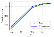
(a) $\kappa$

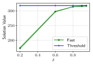
(b) $\delta$

Figure 5: Performance as $\delta$ and $\kappa$ are varied. Note that ThresholdGreedy does not use $\delta$.

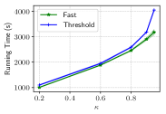
(a) $\kappa$

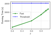
(b) $\delta$

Figure 6: Running time as $\delta$ and $\kappa$ are varied. Note that ThresholdGreedy does not use $\delta$.

In this section, we evaluate the impact of varying the parameters of FastGreedy: $\varepsilon$, $\delta$, and $\kappa$. We note that $\varepsilon$ only impacts the running time and performance if it is used as a stopping condition. However, in our experiments this did not occur: the cardinality constraint was reached first. Therefore, in our experiments FastGreedy = FastGreedy* and we are free to set $\varepsilon=0$ without changing any of our results.

Figures 5 & 6 show the impact of $\delta$ & $\kappa$ on performance and running time. Note that performance remains similar until $\kappa$ or $\delta$ drops below $0.6$. However, the running time plummets to nearly half of what it is at $0.95$ in each case, resulting in a similar-quality solution in significantly less time. A natural follow-up question from this figures is: what happens when both parameters are varied at once? Fig. 7 details the answer. In particular, we note that the steep drop in running time remains present, and there is a reasonable gain to be had by dropping both parameters at once – up to a point.

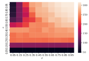
(a) Solution Quality

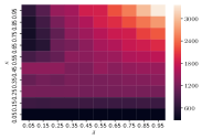
(b) Running Time

Figure 7: Performance and running time of FastGreedy as $\kappa$ and $\delta$ are simultaneously varied.

We further notice some interesting patterns in these heat-maps. When $\kappa$ is near 0, the selection of $\delta$ does not appear to matter. This is likely due to the role each parameter plays: $\kappa$ plays a critical role in identifying a DR-violation, at which point $\delta$ is the rate by which $\beta$ is reduced to compensate. When $\kappa$ is small, it takes commensurately larger violations for $\delta$ to apply. These larger violations are not seen in our simulations, and thus $\delta$ has no impact when $\kappa$ is very small.

Appendix H Implementation Notes

The facebook dataset originally is undirected; we replace each edge $u\leftrightarrow v$ with two edges $u\rightarrow v$ and $v\rightarrow u$.

We calculated the FastGreedy ratio using the values $\kappa=0.95$, $\beta^{*}=0.9$, $\gamma_{s}=0.69857$, $\varepsilon=0$. The values of $\kappa$ and $\varepsilon$ are taken from the parameters used to run the algorithm ($\varepsilon$ can be 0 since the algorithm always returned $\mathbf{g}$ with $\lVert\mathbf{g}\rVert_{1}=k$), and the values of $\beta^{*}$ and $\gamma_{s}$ are the minimum over all instances where FastGreedy Submodularity Ratio was computed.

H.1 Evaluating $\delta_{\mathbf{s}}(\mathbf{g})$

As mentioned in Section 6, we evaluate the objective on a set of 10,000 Monte Carlo samples. However, for performance reasons we do not evaluate the marginal gain $\delta_{\mathbf{s}}(\mathbf{g})$ directly by computing each of $f(\mathbf{g}+\mathbf{s})$ and $f(\mathbf{g})$ and then subtracting. Instead, we compute the expected number of activations across the sample set were $\mathbf{s}$ to be added. We accomplish this as follows.

First, we mantain a state associated with the vector $\mathbf{g}$. This state contains a number of variables for logging purposes, in addition to two of note for our discussion here: samples and active. The former is the list of sampled graphs, each represented as a pair of vectors of floating point numbers corresponding to random thresholds assigned to each node and edge. The latter is a list of sets of nodes currently active in each sampled graph under solution vector $\mathbf{g}$. These active sets are computed only when a new element (or elements) are added to the solution vector and are computed directly by (a) computing the set of externally activated nodes by checking if the random threshold is sufficient to activate the node; then (b) propagating across any active edges according to their thresholds. The code for this is contained in the active_nodes function of src/bin/inf.rs in the code distribution.

Given this representation, to estimate the marginal gain of $\ell$ copies of a node $s$ on each sample $S_{i}$ as follows:

1. Check if the node is already active on $S_{i}$. If so, return 0 for this sample.

2. Check if the node would be externally activated if added to the solution. If not, return 0.

3. Check if the node would be activated by neighboring nodes if added to the solution. If not, return 0.

4. Compute the set of nodes that would be newly activated if $s$ becomes active via breadth-first-search from $s$. Return this number $c$.

Each would-be-activated check is accomplished by comparing the activation probability of the node or edge to the random threshold associated with it in the sample. Then the expected marginal gain is the average result across all samples $S_{i}$. When an element (with multiplicity) is chosen to be inserted into the solution, we add it to the solution vector, discard and recompute all samples, and then recompute the active set on each sample from scratch. This is in line with prior Monte-Carlo-based solutions for IM Kempe et al. [2003].

While in theory it is possible to consider the marginal gain of an arbitrary vector $\mathbf{v}$, in our implementation we restrict the values it can take to $\mathbf{v}=\ell\mathbf{s}$, where $\mathbf{s}$ is the unit vector for node $s$. This simplifies each of the steps above. The implementation of the above is contained in the functions delta and scaled_delta in src/bin/inf.rs.

References

- Alon et al. (2012) Noga Alon, Iftah Gamzu, and Moshe Tennenholtz. Optimizing budget allocation among channels and influencers. Proceedings of the 21st International Conference on World Wide Web (WWW), pages 381–388, 2012. doi: 10.1145/2187836.2187888. URL http://dl.acm.org/citation.cfm?doid=2187836.2187888.
- Badanidiyuru and Vondrák (2014) Ashwinkumar Badanidiyuru and J Vondrák. Fast algorithms for maximizing submodular functions. Proceedings of the 25th Annual ACM-SIAM Symposium on Discrete Algorithms (SODA), pages 1497–1514, 2014. doi: 10.1137/1.9781611973402.110.
- Bian et al. (2017a) An Bian, Kfir Y. Levy, Andreas Krause, and Joachim M. Buhmann. Non-monotone Continuous DR-submodular Maximization: Structure and Algorithms. In Advances in Neural Information Processing Systems (NIPS), pages 486–496, 2017a. URL http://arxiv.org/abs/1711.02515http://papers.nips.cc/paper/6652-non-monotone-continuous-dr-submodular-maximization-structure-and-algorithms.pdf.
- Bian et al. (2017b) Andrew An Bian, Joachim M. Buhmann, Andreas Krause, and Sebastian Tschiatschek. Guarantees for Greedy Maximization of Non-submodular Functions with Applications. In Proceedings of the 34th International Conference on Machine Learning (ICML), 2017b.
- Borodin et al. (2014) Allan Borodin, Dai Tri Man Le, and Yuli Ye. Weakly Submodular Functions. arXiv preprint arXiv:1401.6697, 2014. URL http://arxiv.org/abs/1401.6697.
- Conforti and Cornuéjols (1984) Michele Conforti and Gérard Cornuéjols. Submodular set functions, matroids and the greedy algorithm: Tight worst-case bounds and some generalizations of the Rado-Edmonds theorem. Discrete Applied Mathematics, 7(3):251–274, 1984. ISSN 0166218X. doi: 10.1016/0166-218X(84)90003-9.
- Das and Kempe (2011) Abhimanyu Das and David Kempe. Submodular meets Spectral: Greedy Algorithms for Subset Selection, Sparse Approximation and Dictionary Selection. Proceedings of the 28th International Conference on Machine Learning (ICML), 2011. ISSN <null>. URL http://arxiv.org/abs/1102.3975.
- Demaine et al. (2014) Erik D. Demaine, Mohammad T. Hajiaghayi, Hamid Mahini, David L. Malec, S. Raghavan, Anshul Sawant, and Morteza Zadimoghadam. How to Influence People with Partial Incentives. Proceedings of the 23rd International Conference on World Wide Web (WWW), pages 937–948, 2014. doi: 10.1145/2566486.2568039. URL http://dl.acm.org/citation.cfm?id=2568039.
- Ene and Nguyen (2016) Alina Ene and Huy L. Nguyen. A Reduction for Optimizing Lattice Submodular Functions with Diminishing Returns. arXiv preprint arXiv:1606.08362v1, 2016.
- Feige and Izsak (2013) Uriel Feige and Rani Izsak. Welfare Maximization and the Supermodular Degree. In Proceedings of the 4th conference on Innovations in Theoretical Computer Science (ITCS), pages 247–256, 2013. ISBN 9781450318594. doi: 10.1145/2422436.2422466. URL http://dl.acm.org/citation.cfm?doid=2422436.2422466.
- Gottschalk and Peis (2016) Corinna Gottschalk and Britta Peis. Submodular Function Maximization over Distributive and Integer Lattices. arXiv preprint arXiv:1505:05423, 2016. URL http://arxiv.org/abs/1505.05423.
- Horel and Singer (2016) Thibaut Horel and Yaron Singer. Maximization of Approximately Submodular Functions. In Advances in Neural Information Processing Systems (NIPS), 2016.
- Kempe et al. (2003) David Kempe, Jon Kleinberg, and Éva Tardos. Maximizing the spread of influence through a social network. In Proceedings of the 9th ACM SIGKDD International Conference on Knowledge Discovery and Data Mining (KDD), pages 137–146, 2003. ISBN 1581137370. doi: 10.1145/956755.956769. URL http://portal.acm.org/citation.cfm?doid=956750.956769.
- Krause et al. (2008a) Andreas Krause, Jure Leskovec, Carlos Guestrin, Jeanne M. VanBriesen, and Christos Faloutsos. Efficient sensor placement optimization for securing large water distribution networks. Journal of Water Resources Planning and Management, 134(6):516–526, 2008a. ISSN 0733-9496/2008/6-516–526. doi: 10.1061/(ASCE)0733-9496(2008)134:6(516). URL http://ascelibrary.org/doi/abs/10.1061/(ASCE)0733-9496(2008)134:6(516).
- Krause et al. (2008b) Andreas Krause, Ajit Singh, and Carlos Guestrin. Near-Optimal Sensor Placements in Gaussian Processes: Theory, Efficient Algorithms and Empirical Studies. In Journal of Machine Learning Research, volume 9, pages 235–284, 2008b. ISBN 1390681139. doi: 10.1145/1102351.1102385.
- Lehmann et al. (2006) Benny Lehmann, Daniel Lehmann, and Noam Nisan. Combinatorial auctions with decreasing marginal utilities. Games and Economic Behavior, 55(2):270–296, 2006. ISSN 08998256. doi: 10.1016/j.geb.2005.02.006.
- Leskovec and Krevl (2014) Jure Leskovec and Andrej Krevl. SNAP Datasets: Stanford large network dataset collection. http://snap.stanford.edu/data, June 2014.
- Leskovec et al. (2007) Jure Leskovec, Andreas Krause, Carlos Guestrin, Christos Faloutsos, Jeanne VanBriesen, and Natalie Glance. Cost-effective Outbreak Detection in Networks. In Proceedings of the 13th ACM SIGKDD International Conference on Knowledge Discovery and Data Mining (KDD), pages 420–429, 2007. ISBN 978-1-59593-609-7. doi: 10.1145/1281192.1281239. URL http://eprints.pascal-network.org/archive/00005342/.
- Lin et al. (2017) Yishi Lin, Wei Chen, and John C.S. Lui. Boosting information spread: An algorithmic approach. Proceedings of the International Conference on Data Engineering (ICDE), pages 883–894, 2017. ISSN 10844627. doi: 10.1109/ICDE.2017.137.
- Mirzasoleiman et al. (2015) Baharan Mirzasoleiman, Ashwinkumar Badanidiyuru, Amin Karbasi, Jan Vondrak, and Andreas Krause. Lazier Than Lazy Greedy. In Proceedings of the Twenty-Ninth AAAI Conference on Artificial Intelligence (AAAI), pages 1812–1818, 2015. ISBN 9781577357018. URL http://arxiv.org/abs/1409.7938.
- Soma and Yoshida (2015) Tasuku Soma and Yuichi Yoshida. A Generalization of Submodular Cover via the Diminishing Return Property on the Integer Lattice. Advances in Neural Information Processing Systems (NIPS), 2015. ISSN 10495258.
- Soma and Yoshida (2016) Tasuku Soma and Yuichi Yoshida. Maximizing Monotone Submodular Functions over the Integer Lattice. In Quentin Louveaux and Martin Skutella, editors, Integer Programming and Combinatorial Optimization, pages 325–336, Cham, 2016. Springer International Publishing. ISBN 978-3-319-33461-5. URL http://arxiv.org/abs/1503.01218.
- Soma and Yoshida (2017) Tasuku Soma and Yuichi Yoshida. Non-‐monotone DR-‐Submodular Function Maximization. In Proceedings of the Thirty-First AAAI Conference on Artificial Intelligence (AAAI), pages 898–904, 2017.