A Theory for the Variation of Dust Attenuation Laws in Galaxies
Abstract
In this paper, we provide a physical model for the origin of variations in the shapes and bump strengths of dust attenuation laws in galaxies by combining a large suite of cosmological “zoom-in” galaxy formation simulations with 3D Monte Carlo dust radiative transfer calculations. We model galaxies over orders of magnitude in stellar mass, ranging from Milky Way like systems through massive galaxies at high-redshift. Critically, for these calculations we employ a constant underlying dust extinction law in all cases, and examine how the role of geometry and radiative transfer effects impact the resultant attenuation curves. Our main results follow. Despite our usage of a constant dust extinction curve, we find dramatic variations in the derived attenuation laws. The slopes of normalized attenuation laws depend primarily on the complexities of star-dust geometry. Increasing fractions of unobscured young stars flatten normalized curves, while increasing fractions of unobscured old stars steepen curves. Similar to the slopes of our model attenuation laws, we find dramatic variation in the ultraviolet (UV) bump strength, including a subset of curves with little to no bump. These bump strengths are primarily influenced by the fraction of unobscured O and B stars in our model, with the impact of scattered light having only a secondary effect. Taken together, these results lead to a natural relationship between the attenuation curve slope and bump strength. Finally, we apply these results to a Mpc/ box cosmological hydrodynamic simulation in order to model the expected dispersion in attenuation laws at integer redshifts from . A significant dispersion is expected at low redshifts, and decreases toward . We provide tabulated results for the best fit median attenuation curve at all redshifts.
1 Introduction
Astrophysical dust is pervasive in the interstellar medium (ISM) of most galaxies. This dust can both absorb stellar radiation, as well as scatter light into and out of the line of sight (Witt & Gordon, 2000). Physical properties of galaxies that derive from optical and ultraviolet (UV) radiation, such as the star formation rate (SFR), stellar mass (), and stellar ages must therefore account for these dust-driven effects. Unfortunately, how exactly to do this is complicated (see reviews by Walcher et al., 2011; Conroy, 2013). Beyond the aforementioned effects of extinction and scattering, the spatial distribution between stars of different ages and the dusty ISM (hereafter simply referred to as “the geometry”) can dramatically impact dust attenuation111Following typical convention, we define the following. Extinction measures the loss of photons along the line of sight due to absorption, as well as scattering out of the line of sight. Attenuation refers to extinction, but also taking into account scattering back into the line of sight, as well as the geometric distribution of dust with respect to stars laws in galaxies. These effects are typically described via an attenuation curve, which quantifies the optical depth (), as either a function of wavelength (), or .
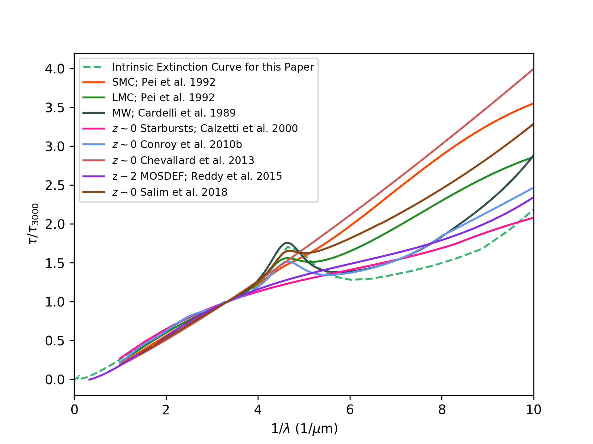
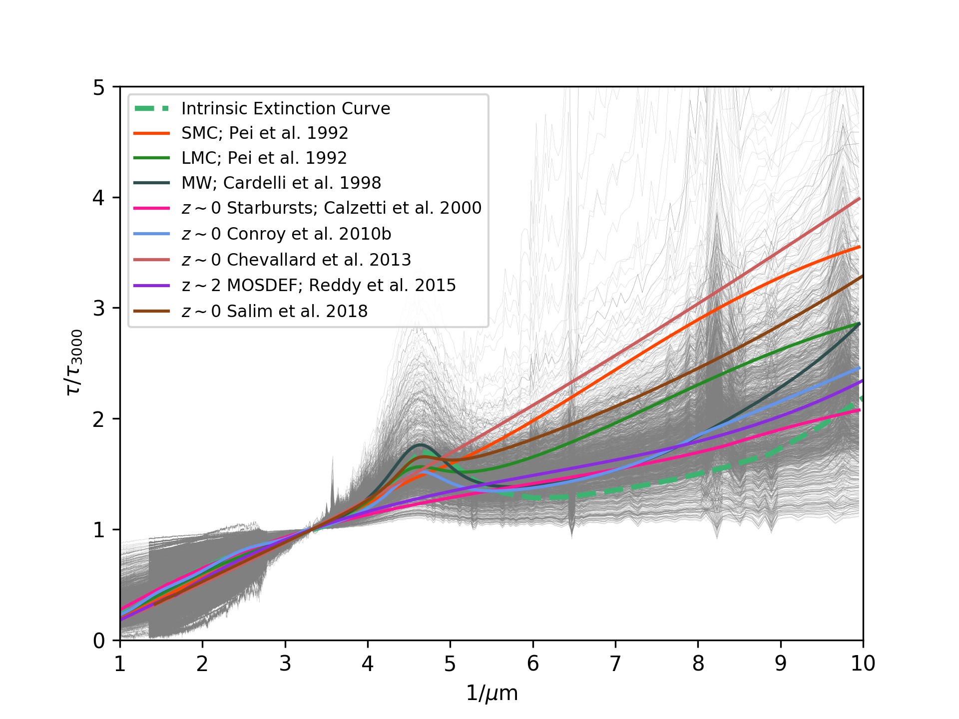
Decades of constraints of observed extinction attenuation curves have evidenced a number of clear features (see reviews by Calzetti, 2001; Draine, 2003; Galliano et al., 2017). First, there is a steep rise toward the ultraviolet due to absorption by small grains such that shorter wavelength photons are preferentially removed from the line of sight. In the near ultraviolet (NUV), there is (sometimes) an absorption bump near , first reported by Stecher (1965), that is potentially associated with polycyclic aromatic hydrocarbons (e.g. Weingartner & Draine, 2001), though some models suggest a graphite-based origin (e.g. Stecher & Donn, 1965; Hoyle & Wickramasinghe, 1962; Draine & Malhotra, 1993), or other species yet (e.g. Wada et al., 1999). This UV bump is known to vary dramatically in strength, a topic we return to later. There is some evidence for an optical knee due to scattering by large grains (Galliano et al., 2017), and the extinction curve takes a powerlaw shape at longer NIR wavelengths. In Figure 1, we show a compilation of a number of literature extinction and attenuation curves that will serve as a useful reference throughout this paper.
These observations have revealed a diversity in derived extinction curves in the Milky Way and nearby galaxies. For example, when parameterizing the inverse of the slope of the extinction curve in the optical as , observations have ranged from values of as low as (Welty & Fowler, 1992) to nearly (Cardelli et al., 1989; Fitzpatrick, 1999). Similarly, Fitzpatrick & Massa (1990) demonstrated a broad range of extinction curves amongst different Milky Way sightlines via International Ultraviolet Explorer (IUE) observations. Cardelli et al. (1989) and Fitzpatrick & Massa (1990) showed that variations in both the attenuation curve shape and UV bump strength can be well-parameterized by the total to selective extinction . The sightline average attenuation curve of the Milky Way has (e.g. Rieke & Lebofsky, 1985). Outside of our galaxy, extinction curves have been measured using this method for the Magallanic clouds, and Andromeda. Pei (1992) and Gordon et al. (2003) derived attenuation curves for the Magallanic clouds, and showed that the Small Magallanic Cloud (SMC) bar, for example, has a steeper curve than the Large Magallanic Cloud (LMC) average when normalizing at optical wavelengths. On average, both of the Magallanic clouds have lower ratios than the Milky Way, which may be due to their lower metallicities (Misselt et al., 1999; Calzetti, 2001). At the same time, Clayton et al. (2015) found that M31 has a relatively similar average curve as the Milky Way.
At larger distances, emission from unresolved stellar populations are measured in aggregate (as opposed to in individual stellar pairs), and the role of star-dust geometry can introduce significant complications. In this regime, constraints on extinction curves become impossible, and instead measurements are made of attenuation curves. When measuring attenuation toward stars in unresolved galaxies (i.e. ), methods include utilizing the ratio of the infrared excess (itself a ratio between the infrared luminosity to a monochromatic UV luminosity) to the UV slope (i.e. the IRX- relation; Meurer et al., 1999; Johnson et al., 2007b; Casey et al., 2014b), color-magnitude diagram fitting (e.g. Dalcanton et al., 2015), and SED fitting techniques (e.g. Papovich et al., 2001; Buat et al., 2011; Kriek & Conroy, 2013; Conroy, 2013; Leja et al., 2017; Salim et al., 2018).
Akin to extinction curves within the Milky Way, attenuation curves in galaxies near and far have shown a dramatic range in observed shapes. In a series of papers, Calzetti et al. (1994); Kinney et al. (1994); Calzetti (1997); Böker et al. (1999) and Calzetti et al. (2000) investigated attenuation laws toward both stars and HII regions in local Universe starburst galaxies. These researchers found that these galaxies, on average, have greyer (also described as ’flatter’ or ’shallower’ throughout this paper) optical/UV attenuation slopes (when normalized in the optical) than the Milky Way, with an average . Johnson et al. (2007a) derive a mean attenuation law in a sample of galaxies of , with little variation when binned by stellar mass. Wild et al. (2011) analyzed galaxies from the Sloan Digital Sky Survey, and found that the slope of attenuation curves varies strongly with galaxy axial ratio, though only weakly with their specific star formation rate. The slopes of these curves vary with stellar mass surface density, with higher stellar mass surface densities correlating with steeper curves. Meanwhile, Battisti et al. (2016) found, for star-forming galaxies at , an average attenuation curve similar to that derived by Calzetti et al. (2000), with an observed range comparable to the factor dispersion in found by Wild et al. (2011). Battisti et al. (2017) expanded on this study, and found little correlation between these curves and a range of galaxy physical properties, including mean stellar age, the specific star formation rate, stellar mass and metallicity. The consensus from local galaxy observations is that, aside from potentially stellar mass surface density (e.g. Wild et al., 2011), there appear to be relatively few correlations between the slope of dust attenuation curves and galaxy physical property.
At high-redshift, the most commonly assumed attenuation curve is a Calzetti et al. (2000) law. Owing to the sensitivity of derived physical parameters on the assumed attenuation law in SED modeling (e.g. Salim et al., 2007), a number of authors have attempted to constrain observed attenuation laws at high-redshift to assess the validity of the typical assumption of a Calzetti et al. (2000) relation. For example, Reddy & Steidel (2004) compared X-ray and radio (i.e. relatively extinction-free) derived SFRs with that derived from Calzetti-corrected UV photometry of UV-selected star forming galaxies between in GOODS-N, and found consistent results. This implies, on average, that an attenuation curve similar to that derived by Calzetti et al. (2000) is a reasonable descriptor of the attenuation properties of these galaxies. A number of other works, using complementary methods, have found reasonable consistency with a Calzetti et al. (2000) attenuation curve at high-redshift (e.g. Scoville et al., 2015; Cullen et al., 2017a; Cullen et al., 2017b). Much of this work has focused on the location of galaxies at high-redshift on the IRX- plane, and their consistency with a Calzetti et al. (2000) attenuation curve (e.g. Seibert et al., 2002; Reddy et al., 2008; Pannella et al., 2009; Siana et al., 2009; Reddy et al., 2012; Heinis et al., 2013; To et al., 2014; Bourne et al., 2016; McLure et al., 2017).
At the same time, Reddy et al. (2015) derived attenuation curves for galaxies from the MOSFIRE Deep Evolution Field (MOSDEF) survey, and found evidence for a composite attenuation curve that is similar to the Calzetti et al. (2000) form at short wavelengths, and the SMC extinction curve at . Similarly, Lo Faro et al. (2017) find evidence for a composite attenuation curve in a sample of galaxies selected for their infrared luminosity. Salmon et al. (2016) found a diverse range of attenuation laws in galaxies from the CANDELS survey with little correlation with galaxy physical property, and Shivaei et al. (2015) required curves steeper than Calzetti et al. (2000) to match the observed IR/UV ratios in star-forming galaxies. And, in the same vein, dramatic outliers from the Meurer et al. (1999) IRX- relation at high-redshift have pointed to underlying variations in attenuation laws. This said, other complicating factors may contribute to deviations from the locally calibrated Meurer et al. (1999) relation (e.g. Bell et al., 2002; Kong et al., 2004; Grasha et al., 2013; Koprowski et al., 2016; Safarzadeh et al., 2017; Popping et al., 2017b; Narayanan et al., 2018).
Similar to variations in the attenuation curve slope, galaxies in both the local Universe and at high-redshift exhibit a wide range of UV absorption bump strengths. Both the SMC and average attenuation curve for nearby starburst galaxies lack strong bump features (Gordon et al., 2000; Calzetti et al., 2000), and Gordon et al. (1999) find relatively small bump strengths in attenuation curves for a sample of high-redshift galaxies from the Hubble Deep Fields. Meanwhile, a number of studies at both low redshift (Conroy et al., 2010b; Wild et al., 2011; Battisti et al., 2016; Salim et al., 2018), and high- (Motta et al., 2002; Burgarella et al., 2005; York et al., 2006; Stratta et al., 2007; Noll et al., 2007, 2009; Elíasdóttir et al., 2009; Buat et al., 2011; Scoville et al., 2015) have found evidence of absorption bumps of varying strengths. A substantial step forward was made by Kriek & Conroy (2013), who not only demonstrated evidence of a bump in the attenuation curves of star-forming galaxies, but also that the bump strength varies with the slope of the attenuation curve (such that the steepest curves have the strongest bumps).
Given the strong dependence on inferred galaxy physical properties on attenuation curves, understanding the origin of their shape variations is critical. Here, modeling can provide significant insight as to the physical drivers of variations in both attenuation law slopes and feature strengths. Models designed to understand attenuation laws in galaxies generally fall into one of three methodology camps. The core of each involves radiative transfer modeling of stellar light through a dusty interstellar medium, and the primary difference lies in how the geometry of stars and the dust is modeled. The general trade off is that increases in model complexity are typically associated with increased astrophysical realism, though decreased ability to develop controlled numerical experiments.
The most simplified models typically involve illuminating a slab or shell-like geometry with a stellar radiation source. Early works include Witt & Gordon (1996, 2000), who used these models to demonstrate that increasingly mixed star-dust geometries result in flatter (grayer) attenuation curves. Seon & Draine (2016) expanded upon these significantly by developing a model for a turbulent ISM with a lognormal density profile and a clumpy medium to investigate the origin of attenuation law shape and bump strength variations. While these models can neatly isolate individual physical effects, they do not model galaxies as a whole, taking into account the radiative transfer from stars with a distribution of stellar ages and metallicities through a cosmologically evolved interstellar medium.
The latter two modeling categories analyze attenuation laws for galaxies as a whole. These include hydrodynamic simulations of idealized galaxies evolving without a cosmological context, and simulations that employ semi-analytic modeling techniques within a cosmological framework. In the former category, Jonsson (2006); Rocha et al. (2008); Natale et al. (2015); Hayward & Smith (2015) and Hou et al. (2017) coupled idealized models of isolated disk galaxies and galaxy mergers with 3D dust radiative transfer to model their dust attenuation properties. Such simulations can achieve very high resolution, but do not include the hierarchical growth of galaxies that can result in more diverse (and realistic) morphologies (e.g. Abruzzo et al., 2018) leading to variations in dust attenuation. This is especially true at early epochs when dusty disks are thicker and clumpier, and are responding dynamically to high rates of gas inflows and outflows. Meanwhile, semi-analytic models (SAMs) have been developed to model dust attenuation in a cosmological context (e.g. Granato et al., 2000; Fontanot et al., 2009; Fontanot & Somerville, 2011; Gonzalez-Perez et al., 2013; Wilkins et al., 2012). Such models do not track baryonic growth directly, but rather track dark matter growth and make physically-motivated but simplistic assumptions about the resulting galaxy properties. The benefit is that, when coupled with spectrophotometric dust radiative transfer calculations, SAMs are able to efficiently produce cosmological volumes of galaxies with SED information. But since the baryonic matter is characterized through analytic expressions (e.g. Popescu et al., 2011), the geometry of the ISM and stars is not directly predicted but rather based on simplified assumptions.
What is missing thus far is a theoretical interpretation of dust attenuation laws in the context of models that directly track the hydrodynamic growth and evolution of galaxies from cosmological conditions with sufficient resolution to model the impact of complex star-dust geometries. Cosmological hydrodynamic simulations are attractive in their ability to directly track the hierarchical growth of galaxies, and therefore provide relatively realistic star-dust geometries for stellar populations with a distribution of metallicities and formation ages. In this paper, we present the first ever theoretical model for dust attenuation curves in galaxies from cosmological hydrodynamic simulations.
To do this, we will employ the cosmological “zoom” technique, where we focus on individual halos (and their associated baryons) in cosmological simulations at very high resolution. We couple these simulations with 3-dimensional dust radiative transfer to model how the intrinsic stellar light is absorbed and scattered, and consequently develop a model for dust attenuation laws in galaxies. Critical to the interpretation of our results: in this model, we will assume an underlying dust extinction law (i.e. we will hold the properties of dust grains fixed), and ask how geometry and radiative transfer effects drive variations in the attenuation law slope and UV bump strength. In § 2 we describe our simulation setup; in § 3 we build physical insight via simplified population synthesis models; in § 4, we apply this insight to direct results from cosmological zoom galaxy formation simulations. Here, we explore the origin of variations in the slope and the bump strength in attenuation laws in galaxies. In § 5 we provide discussion, and we summarize in § 6. Throughout, we assume a cosmology of ) = .
|
2 Simulation Methodology
2.1 Overview
In order to model dust attenuation curves, we must know both the intrinsic stellar spectrum in model galaxies, as well as the observed SED. To generate these, we first simulate a series of model galaxies using the cosmological zoom technique. We then determine the stellar SEDs for these model galaxies based on the individual metallicities and ages for the star particles via fsps calculations. These stellar SEDs are propagated through the dusty interstellar medium via hyperion dust radiative transfer (wrapped in the powderday code package), and compared to the final observed attenuated UV-optical SED in order to determine the attenuation curve. The underlying extinction properties of the grains are fixed throughout, and we utilize the aforementioned simulations to understand the impact of dust geometry and radiative transfer effects on the observed attenuation curves.
2.2 Cosmological Zoom Galaxy Formation Simulations
Our model galaxy suite is generated from the mufasa-zoom simulation series, which are zoomed galaxies from the mufasa cosmological simulation (Davé et al., 2016, 2017a, 2017b). This zoom simulation methodology has been described in detail in Olsen et al. (2017), Narayanan et al. (2018), Abruzzo et al. (2018), and Privon et al. (2018). We therefore refer the reader to those works for details, and summarize the salient points here.
All of our simulations are conducted with a modified version of the gizmo hydrodynamic code (Hopkins, 2015, 2017), which builds off of the code base in gadget-3 (Springel et al., 2005). We first simulate a coarse resolution dark matter only run from down to using initial conditions generated from music (Hahn & Abel, 2011). The initial conditions for this dark matter box are the exact same as those used in the mufasa cosmological hydrodynamic simulation. This coarse resolution run is done in a Mpc volume, and includes dark matter particles, resulting in dark matter mass resolution of . It is from this dark matter only simulation that we select our model halos to re-simulate at much higher resolution (and with baryons included).
We re-simulate eight halos over a broad mass range to final redshifts , where varies based on the halo mass. Five of these halos are described in Narayanan et al. (2018), and we have include three additional models in this paper. In Table 1, we describe their physical properties222We order the simulations in Table 1 by their halo mass. In the case of halo , which did not reach , we order in terms of its expected mass from the parent dark matter cosmological simulation., and present their location in stellar mass-halo mass space and SFR- space in Abruzzo et al. (2018). These simulations span roughly three decades in halo mass, and represent galaxies ranging from Milky Way mass (at ) through halo masses comparable to luminous dusty galaxies at (e.g. Narayanan et al., 2015; Casey et al., 2014a).
We identify halos using caesar (Thompson, 2014). For each halo of interest for resimulation, we build an ellipsoidal mask around all particles encapsulating a radius the distance of the farthest particle from halo center, and define this as the Lagrangian region for resimulation. We then track these particles back to , split these to the desired resolution, and re-run the simulation to with hydrodynamics turned on. We have zero low-resolution particles contaminating any halo presented here within three virial radii.
Our simulations use the suite of physics developed for the mufasa cosmological hydrodynamic simulations (Davé et al., 2016, 2017a, 2017b). Here, stars form in dense molecular gas, and the H2 fraction is calculated using the Krumholz et al. (2009) methodology, tying the molecular fraction to the gas surface density and metallicity (Thompson et al., 2014). We impose a minimum metallicity for star formation of . This star formation occurs at a rate following a volumetric Schmidt (1959) relation, with an imposed efficiency per free fall time of , as motivated by observations (Kennicutt, 1998; Kennicutt & Evans, 2012; Narayanan et al., 2008, 2012; Hopkins et al., 2013).
Feedback from massive stars are modeled via the mufasa decoupled two-phase wind scheme. The wind physics are presented in detail in Davé et al. (2016), and we refer the reader to that work for a full description of the wind model. Briefly, the modeled stellar winds have a probability for ejection that is modeled as a fraction of the SFR probability. This fraction is derived from the best-fitting relation from the Feedback in Realistic Environments (Muratov et al., 2015; Hopkins et al., 2014, 2017) simulation suite. The dependence of the ejection velocity on the galaxy circular velocity also derives from the Muratov et al. (2015) high-resolution simulations. The circular velocities are determined on the fly using a fast friends-of-friends finder (Davé et al., 2016).
Feedback from longer-lived stars (e.g. asymptotic giant branch stars [AGB] and Type 1a supernovae) are included as well (following Bruzual & Charlot (2003) stellar evolution tracks with a Chabrier (2003) initial mass function). We track the evolution of 11 elements: H, He, C, N, O, Ne, Mg, Si, S, Ca and Fe. The yields for SNe Ia are taken from Iwamoto et al. (1999), assuming of returned mass per supernova event. AGB yields are drawn from the Oppenheimer & Davé (2008) lookup tables. Type II supernovae yields derive from Nomoto et al. (2006) parameterizations, though are reduced by owing to studies that find these yields return galaxies with metallicities roughly a factor too large at a fixed stellar mass when compared to the observed mass-metallicity relation (Davé et al., 2011).
The hydrodynamic simulations all use gizmo in the meshless finite mass mode (MFM), with a cubic spline of neighbors in the MFM hydrodynamics. This kernel is used to define the volume partition between gas elements, and the faces therefore over which the hydrodynamics is solved with the Riemann solver. Our final particle masses are as follows. The dark matter particle masses are , and baryon particle masses are . We employ adaptive gravitational softening for all particles throughout the simulation with minimum force softening lengths of and pc for dark matter, gas and star particles respectively.
| Name | ) | ) | ||
|---|---|---|---|---|
| mz0 | 2.15 | |||
| mz5 | 2 | |||
| mz45 | 2 | |||
| mz10 | 2 | |||
| z0mz352 | 0 | |||
| z0mz401 | 0 | |||
| z0mz287 | 0.65 | |||
| z0mz374 | 0.4 |
2.3 Dust Radiative Transfer Models
We generate the stellar SEDs and subsequent dust radiative transfer with powderday, a code package that wraps fsps (Conroy et al., 2009, 2010a; Conroy & Gunn, 2010), hyperion (Robitaille, 2011) and yt (Turk et al., 2011). This process is performed on all snapshots at redshifts in post-processing.
We generate the stellar SEDs using fsps, and in particular, their python hooks python-fsps333https://github.com/dfm/python-fsps. The SEDs are calculated for each star particle as a simple stellar population based on its age and metallicity, which is taken directly from the hydrodynamic simulations. We assume a Kroupa (2002) stellar IMF for the stellar SED generation, and the Padova stellar isochrones (Marigo & Girardi, 2007; Marigo et al., 2008). The sum of these stellar SEDs comprise the intrinsic stellar SED for any given model galaxy snapshot.
We then calculate the attenuation these SEDs experience by performing dust radiative transfer calculations. Functionally, the radiative transfer must occur on a grid. We therefore project the metal mass from the hydrodynamic simulations onto a kpc octree grid centered on the central galaxy’s center of mass. Each cell is recursively subdivided until a maximum of particles are in a cell. The dust mass is assumed to be a constant the metal mass within a cell, as motivated by observational constraints from both local epoch galaxies and those at high-redshift (Dwek, 1998; Vladilo, 1998; Watson, 2011).
The radiative transfer from stellar sources occurs in 3 dimensions in a Monte Carlo fashion using the dust radiative transfer code hyperion (Robitaille, 2011). hyperion uses the Lucy (1999) algorithm for determining the converged equilibrium dust temperature and radiation field. Here, radiation is emitted from stellar sources and then absorbed, scattered, and re-emitted from dust in each cell in the octree grid. This process is iterated upon until the dust temperature has converged; convergence is determined when the energy absorbed by per cent of the cells has changed by less than per cent between iterations. We compute the emergent intensity for isotropic viewing angles around our model galaxies.
For the dust grain properties themselves, we utilize the carbonaceous-silicate grain model from Draine & Li (2007) with a size distribution from Weingartner & Draine (2001). This model uses the Draine (2003) renormalization relative to H and we assume . This curve is shown as a reference in Figure 1.
3 Insight from Simplified Toy Models
|
|
|
|
We begin the analysis for this paper by first conducting a series of simplified stellar population synthesis numerical experiments. It is from these that we will build the physical intuition necessary to understand the results of significantly more complex systems (i.e. the cosmological zoom galaxy formation simulations).
The relevant parameters in the dust attenuation curve for SED modeling are its normalization and its shape. The overall normalization is trivially a function of the total dust column density seen by stars. As a result, we do not explore this further, and concentrate hereafter on the shape of the attenuation curve.
When considering the shape (i.e. slope) of the attenuation curve, we assert that three principle physical drivers are at play: (i) the shape of the underlying extinction curve (which, itself, is dictated by the dust grain size distribution), the (ii) the star-dust geometry, and the (iii) the average stellar age. We demonstrate the first (grain size variations) effect in Figure 2, the second effect (star-dust geometry) in Figure 3, and the final effect (stellar ages) in Figures 4-5.
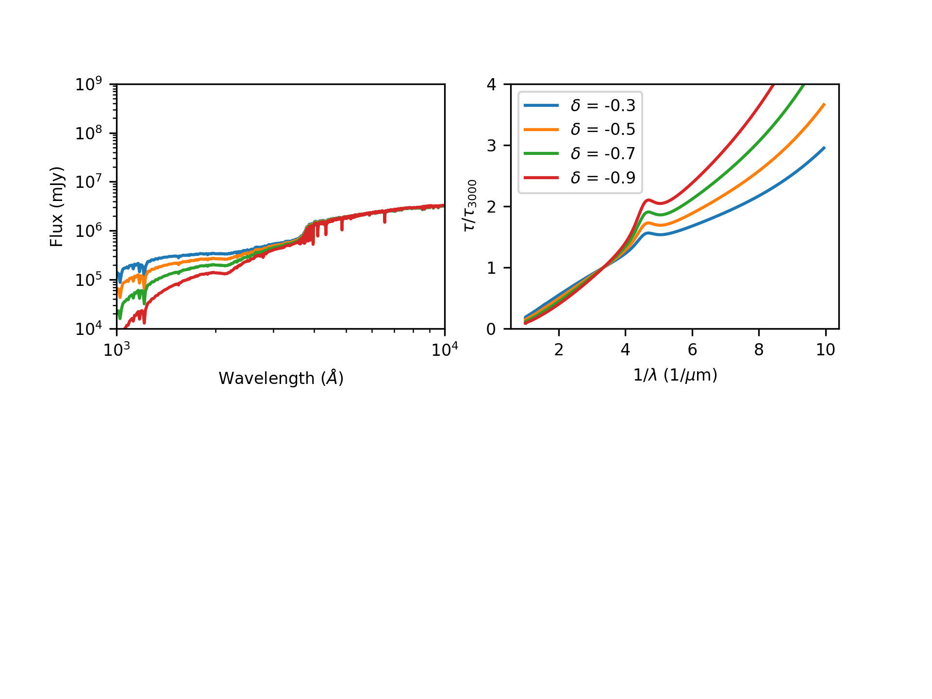
In Figures 2 and 3, we create (as an extreme example) a stellar population with fsps (Conroy et al., 2009, 2010a; Conroy & Gunn, 2010) with age Gyr formed with a constant yr-1 star formation history. Stars reside behind a dust screen whose opacity varies as a function of stellar age. Following Charlot & Fall (2000), we take:
| (1) |
such that the dust screen in front of the stellar population in this experiment has a variable age-dependent normalization. Here, we set the normalization for young stars ( yr) as , while older stellar populations see a normalization (see Conroy et al., 2010a). Following Charlot & Fall (2000), we set . The strong attenuation for young stars is intended to emulate the attenuation of starlight from newly formed stars by their birthclouds, while the more modest attenuation for older populations serves as a proxy for diffuse cirrus dust in galaxies. The extinction curve follows the Kriek & Conroy (2013) derived curve444Formally, the Kriek & Conroy (2013) curve is an attenuation curve. For these models, we use it as an extinction curve, though note that our results are robust against using a wide range of extinction curves. One aspect of the Kriek & Conroy (2013) curve that is visible in Figure 2 (though unimportant for this particular experiment) is that the bump strength manifestly varies with the slope powerlaw index. We further note that the choice of a Kriek & Conroy (2013) curve is only used for the numerical experiments in this section.
In Figure 2, we vary the slope of the imposed Kriek & Conroy (2013) extinction curve as a proxy for variations in the underlying dust grain properties, and hold the dust covering fraction fixed at unity (meaning all stars see the dust screen). It is evident that variations in the intrinsic extinction curve propagate to a wide range of observed attenuation laws. At the same time, absent a model for the physical evolution of dust grain properties in cosmologically evolving galaxies (e.g. McKinnon et al., 2016; Popping et al., 2017a; Hou et al., 2017), we are forced to assume a fixed underlying extinction curve, and do not consider variations that originate in the physics of dust grain property variations further. We instead focus on the impact of the star-dust geometry and stellar ages on the shape of the normalized attenuation curve.
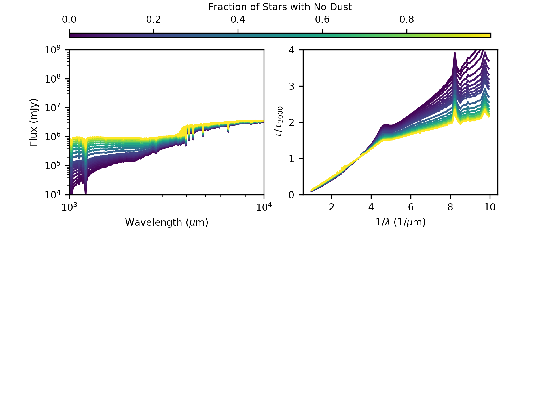
In Figure 3, we show a similar model as in Figure 2, though fix the slope of the Kriek & Conroy (2013) extinction curve () and instead vary the fraction of stars that do not see any dust. This model is intended to serve as a proxy for increasingly complex star-dust geometries in galaxies. A simplified geometry where all stars are enshrouded by dust is represented by a fraction of , while a model in which the stellar light and dust clouds are wholly decoupled is represented by a fraction . As the star-dust geometry becomes increasingly complex, and more of the star light is decoupled from dust, the effective attenuation curve becomes flatter (greyer), a well known result dating back to seminal works by Witt & Gordon (1996).
Note that a ’complex star-dust geometry’ can encapsulate a broad range of effects. For example, a system that has a significant young stellar population that dominates the UV and is enshrouded in dust, but also a significant unobscured old star population that dominates the optical will have a maximally steep attenuation curve. On the other hand, a galaxy with a significant unobscured young star population (e.g. Casey et al., 2014b; Geach et al., 2016; Narayanan et al., 2018), but obscured old star population would have an extremely shallow (grey) attenuation curve. Intermediate cases naturally fall between these two limits.
Because of this, alongside the typical star-dust geometry, the median stellar age of a galaxy can impact observed dust attenuation curves as well. In short: galaxies with a young median stellar age have both their UV and optical light dominated by young stars. Hence, the shape of the attenuation curve in this situation is dictated primarily by the fraction of obscured young stars. Galaxies with an older median stellar age, however, represents a different situation. Here, the optical light is typically dominated by older stars, which tend to be free from obscuring dust, while the UV light is still dominated by young stars. In this case, the ultraviolet regime in the attenuation curve is dictated by the fraction of obscured young stars, while the optical is determined by the fraction of obscured old stars.
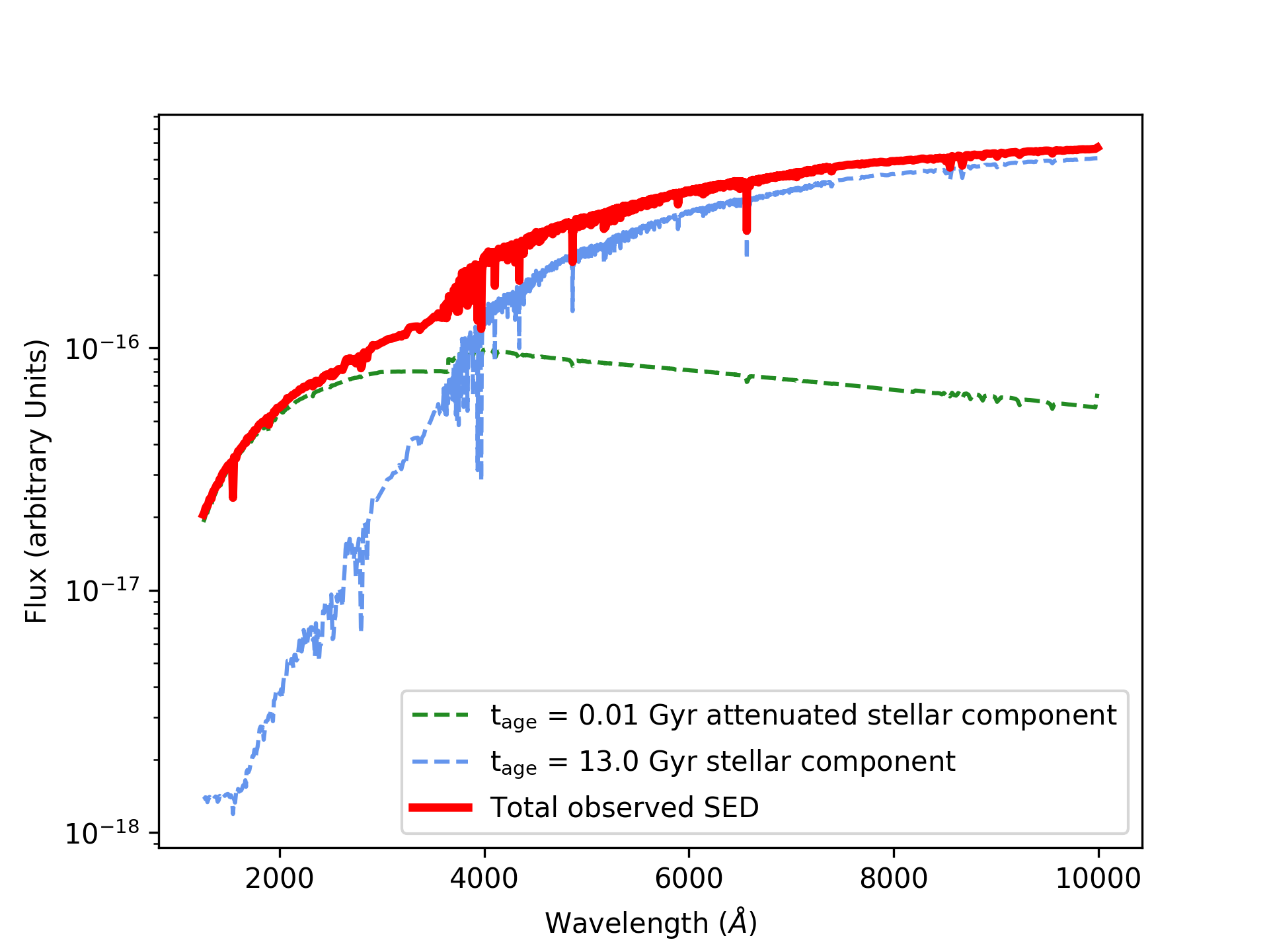
To see this explicitly, we develop a simplified population synthesis experiment in Figure 4. Here, we have constructed a composite stellar population (red line) comprised of a Gyr population (green line) and a Gyr population (blue line). The Gyr population constitutes % of the total mass, and the Gyr population constitutes the remaining . The intention behind this contrived experiment is to mimic a galaxy comprised principally (to the level) of old stars, with only residual ( of the total mass) current star formation. As usual in our population synthesis numerical experiments, the young stars are hidden behind a Charlot & Fall (2000) screen of dust with the same parameters used thus far. The old stars do not suffer any dust attenuation.
Evident in Figure 4 is that the new stars (that suffer attenuation from a dust screen) dominate the SED at FUV wavelengths, while the older stellar population dominates the optical. Because the older stars do not see a dust screen, this will result in increased transparency at optical wavelengths, though depressed emission at FUV wavelengths (thanks to the young stars hidden behind the Charlot & Fall (2000) screen). This scenario can therefore play an important role in determining the shape of normalized attenuation curves.
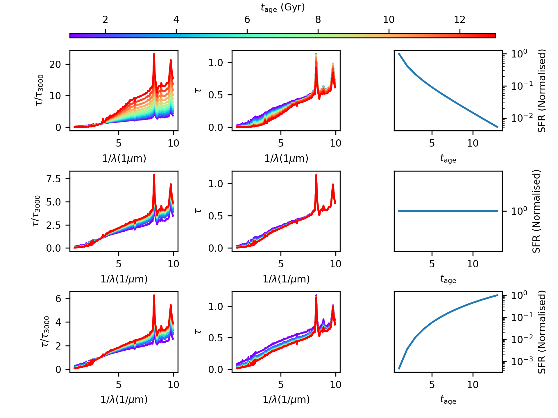
To demonstrate the impact of stellar ages on the normalized attenuation curves even further, in Figure 5, we increase the complexity of the numerical experiments developed in Figure 4, and model three different star formation histories in population synthesis models. The top row shows an exponentially declining SFH, the middle row a constant SFH, and the bottom row a rising SFH; the SFH for each is quantified in the last (third) column. As in all simplified population synthesis experiments developed thus far in this paper, in Figure 5, we utilize the Charlot & Fall (2000) type dust model, where young stars reside behind a dust screen, though evolved stars do not.
In the first and second columns, we show the normalized and absolute attenuation curves for a range of stellar ages. The third column shows the star formation history. Let us first consider the case of the exponentially declining star formation history (row 1) as an instructive example. When examining the first column of the first row (normalized attenuation curves), we see that the models with the oldest ages have the steepest normalized curves. The reason for this becomes evident in the second column (absolute attenuation curve). As the star formation history evolves in the top row of Figure 5, the obscuration of the sources that dominate the far ultraviolet (FUV; ) photons doesn’t change (thanks to the assumption of Charlot & Fall (2000) birth clouds), but that of the optical photons does. Galaxies with more evolved stellar populations still have their UV fluxes dominated by young stars, though their optical fluxes derive instead from older stellar populations. What this means is, if young stars are generally more obscured than older stars (in the stellar population synthesis models explored here, this is manifestly enforced), then galaxies with young median stellar ages will see significant obscuration in both the UV, as well as the optical. Galaxies that are more evolved will still see significant obscuration in the UV (as the young stars are still enshrouded in dust), though the older stars that dominate the optical have lower optical depths (column 2 of Figure 5), and therefore steeper normalized attenuation curves.
The same effects are visible in the second and third rows of Figure 5 (constant and rising SFH, respectively). This said, the dispersion in attenuation curve slopes is more modest compared to the exponentially declining history owing to the mixed contribution to optical light by both young and older stellar populations in the most evolved ( Gyr) stellar age bin.
4 Dust Attenuation Curves in Cosmological Galaxy Formation Simulations
With the insight we have built from our simplified stellar population synthesis models in § 3, we now turn to the modeled curves in our cosmological zoom galaxy formation simulations. As a reminder: going forward we will hold the underlying dust extinction properties fixed with a Weingartner & Draine (2001) size distribution. Beyond this, because the inclusion of subresolution birth clouds depends on tunable free-parameters that can impact the amount of attenuated light (e.g. Narayanan et al., 2009, 2010; Hayward et al., 2013) we will abandon the usage of any subresolution ’birthcloud’ model in the zoom simulations. All attenuation seen by stars will be on larger scales ( pc) from the geometry of the galaxy itself.
4.1 Diversity in Dust Attenuation Curves
To set the stage, in Figure 6, we show the diversity of attenuation curves for all snapshots of all model zoom galaxy formation simulations examined in this paper. The attenuation curves are normalised by their optical depth (which, hereafter, we refer to as ). We additionally show a number of observationally-constrained literature attenuation curves for reference. It is clear that a wide range of attenuation curves emerge from these simulations, with curves both steeper and grayer (shallower) than the standard literature assumptions. The goal of the remainder of this section is to unpack these curves further, and examine in detail the physical drivers behind this diversity in attenuation curves.
|
4.2 Fitting Parameterizations
In our analysis of the physical drivers of the shapes of attenuation curves, we begin by describing formulae that we employ to fit our model attenuation curves. It is useful to go through this exercise at this point, as this will allow us to introduce variables that we can use to characterize various properties of the modeled attenuation curve (e.g. their UV bump strengths, or the normalized slope of the attenuation curve).
Broadly, we follow a modified version of the parameterizations described in Conroy et al. (2010a), which themselves are a modified version of the Cardelli et al. (1989) fits to the average Milky Way extinction curve. For the UV bump, we utilize a Drude profile, and in the near ultraviolet (NUV), we follow Noll et al. (2007).
In more detail, we first define as the inverse wavelength with units of m. We fit the infrared () with:
| (2) | |||
| (3) | |||
| (4) |
In the optical (), we define:
| (5) |
and then parameterize the optical via:
| (6) | |||
| (7) | |||
| (8) |
The near ultraviolet (NUV) and UV bump are modeled via a Calzetti et al. (2000) law, with a Lorentzian-like Drude Profile. The latter is given by:
| (9) |
where is the central wavelength of the bump, is the width, and is the amplitude (Fitzpatrick & Massa, 2007; Noll et al., 2009). Formally, the fit for the NUV and bump take the form:
| (10) |
Here, is a normalization of the fit, and is the Calzetti et al. (2000) law over the wavelengths of interest. The term allows for an arbitrary tilt to the curve in this wavelength regime, and the term compensates for how will change in the original Calzetti law due to the introduction of a tilt Noll et al. (2009).
Finally, we model the far ultraviolet (FUV) between via:
| (11) | |||
| (12) | |||
| (13) | |||
| (14) | |||
| (15) |
In other parameterizations of attenuation curves (e.g. Conroy et al., 2010a), is a parameter describing the bump strength. Because we employ the Noll et al. (2009) model for the NUV and bump, here (in the FUV), serves simply as another free parameter in the fit. In this wavelength regime, we linearly interpolate over the Ly line to avoid complications during fitting.

|
We note that while a piece-wise fit to attenuation curves akin to what is presented here has been used regularly in the literature (e.g. Cardelli et al., 1989; Conroy et al., 2010a), a number of studies in the literature make use of a modified Calzetti et al. (2000) curve over the entire m wavelength range:
| (16) |
where is the Calzetti et al. (2000) relation, is the index for a power-law modification to this relation, is the normal Drude profile (to represent the bump), and is a constant free parameter. Various forms of this relation exist in the literature, where the constant may be multiplied by all or only some of the terms in Equation 16. is a constant that typically relates either or to the ratio of total to selective extinction for the Calzetti et al. (2000) relation (i.e. ), but the exact implementation of this also varies in the literature (e.g. Noll et al., 2009; Kriek & Conroy, 2013; Salmon et al., 2016; Salim et al., 2018). Similarly, not all authors include the Drude representation of a bump. In order to compare against observations, we will find it useful at times in this paper to employ Equation 16 to fit over the entire wavelength regime of the attenuation curve. In this case, we will note the power-law indices used in this case as , instead of , which we shall reserve for our normal fitting procedure.
Beyond this, some authors fix the width () of the Drude profile representing the bump strength. In this situation, we denote the normalization of the bump as , and the width of the bump as :
| (17) |
For clarity, we collect the fitting variables from this section that we will employ to compare with observations in Table 2.
| Fitting Variable | Definition | Equation |
|---|---|---|
| Power law index in NUV wavelength range | Equation 10 | |
| Power law index of modified Calzetti et al. (2000) curve | Equation 16 | |
| Integral of Drude Profile in NUV: bump strength | Equation 9 | |
| Normalization of UV bump, given a variable bump width | Equation 9 | |
| Normalization of UV bump, assuming a constant bump width, | Equation 17 | |
| Value of constant bump width for | Equation 17 |
4.3 What Sets the Slope of Dust Attenuation Curves?
Building from our intuition in § 3, we examine the physical drivers of the slopes of our model dust attenuation curves. Fundamentally, the principal driver of variations in the slope of attenuation curves is the star-dust geometry. Recalling § 3, the steepest attenuation curves arise from galaxies with a significant fraction of young stars (dominating the emitted UV flux) obscured by dust, but old stars (dominating the optical flux) that are not obscured. A more mixed geometry (i.e. more old stars obscured by dust, or more young stars decoupled from dust) will flatten the attenuation curve from this extreme limit. In § 3, we showed this explicitly with simplified population synthesis models; we now explore these effects in bona fide cosmological galaxy formation simulations. We center this discussion around Figure 7 where we show various incarnations of the attenuation curves of an example model galaxy, model mz10.
In the top left panel of Figure 7, we show the normalized attenuation curves for model mz10, color-coded by their fraction of unobscured young stars. This quantity is determined by calculating the fraction of stellar mass in the form of young ( Myr) stars that have no dust within pc. In other words, larger values of this fraction correspond with increasingly decoupled geometry between young stars and dust in galaxies. To minimize the complicating effects of older stellar populations (an effect we will return to shortly), we only plot the attenuation curves for galaxies with a median stellar age (by mass) Gyr; this said, in light grey we show the attenuation curve for all snapshots of this model (i.e. of all median stellar ages). While the dynamic range in attenuation curve slopes is relatively small, it is clear from the top left panel of Figure 7 that a larger fraction of unobscured young stars results in a flatter dust attenuation curve.
Similarly, the geometry between old stars and dust also plays a role in the tilt of observed attenuation curves. To demonstrate this, in the top right panel of Figure 7, we show the same attenuation curves as shown in the top left panel, though in this case we color-code the attenuation curves by their fraction of unobscured old stars. As in the top left panel, we define ’unobscured’ as having no dust within pc, and old stars as those with Myr. To minimize contamination by young stellar populations, we only include galaxies with median stellar age Gyr, though show the curves for all snapshots in light grey. As in the simplified stellar population synthesis models presented in Figure 5, galaxies that contain a significant amount of old stars that are unobscured by dust have steep attenuation curves, while those that have larger obscuration of old stars have flatter (greyer) attenuation curves.
Why are the curves in the top left panel of Figure 7 that are associated with young galaxies uniformly shallower (greyer) than the older stellar age curves on the top right of Figure 7? As shown in Figures 4-5, in galaxies where the median stellar age is relatively young, the UV and optical light are both dominated by newly formed stars. If the light from these stars is attenuated by dust, then both the optical and UV emission from the galaxy will be attenuated. As a result, these curves will not be as steep as a situation where young stars (that are obscured) dominate the UV emission, but old stars are relatively unobscured (a situation described by the top right panel of Figure 5.
What this results in is a situation where galaxies with older stellar ages, on average, have steeper attenuation curves. In the bottom left panel of Figure 7, we show this by plotting the same attenuation curves as in the other two panels, though this time color-coded by the median stellar age. As the galaxy age increases, so does the slope. This is due to an increasingly large fraction of the optical emission coming from older stars as the galaxy ages. Older star particles, on average, are less likely to be associated with dust than young stars. This same effect was noted by Charlot & Fall (2000), who noted steeper attenuation curves with increasing galaxy age.
4.4 Variations in the Bump
As discussed in § 1, while one of the strongest features in the attenuation curve of the Milky Way is the bump feature observed at , a number of observations show dramatic variations in bump strength in different galaxies (e.g. Gordon et al., 1999; Gordon et al., 2000; Calzetti et al., 2000; Motta et al., 2002; Burgarella et al., 2005; York et al., 2006; Stratta et al., 2007; Noll et al., 2007; Elíasdóttir et al., 2009; Conroy, 2010; Buat et al., 2011; Wild et al., 2011; Kriek & Conroy, 2013; Scoville et al., 2015; Battisti et al., 2016; Salim et al., 2018). In this section, we utilize the model that we have developed thus far to understand the origin of variations in the UV bump strength in galaxy attenuation curves.
We define the strength of the UV bump as the integral over the best fit Drude profile in the NUV (c.f. Equation 9):
| (18) |
Note that literature definitions of the bump strength vary, with some definitions characterizing the strength as (i.e. one numerator term in Equation 9), as well as , where the width of the bump is held fixed; c.f. Table 2.
Because the UV bump is an absorption feature, for a fixed underlying extinction curve, reduced bump strength in the observed attenuation curve signifies extra radiation filling in the bump. In principle, there are two possible sources of this extra radiation: light being scattered into the line of sight, and unobscured sources of UV radiation (i.e. unobscured young stars).
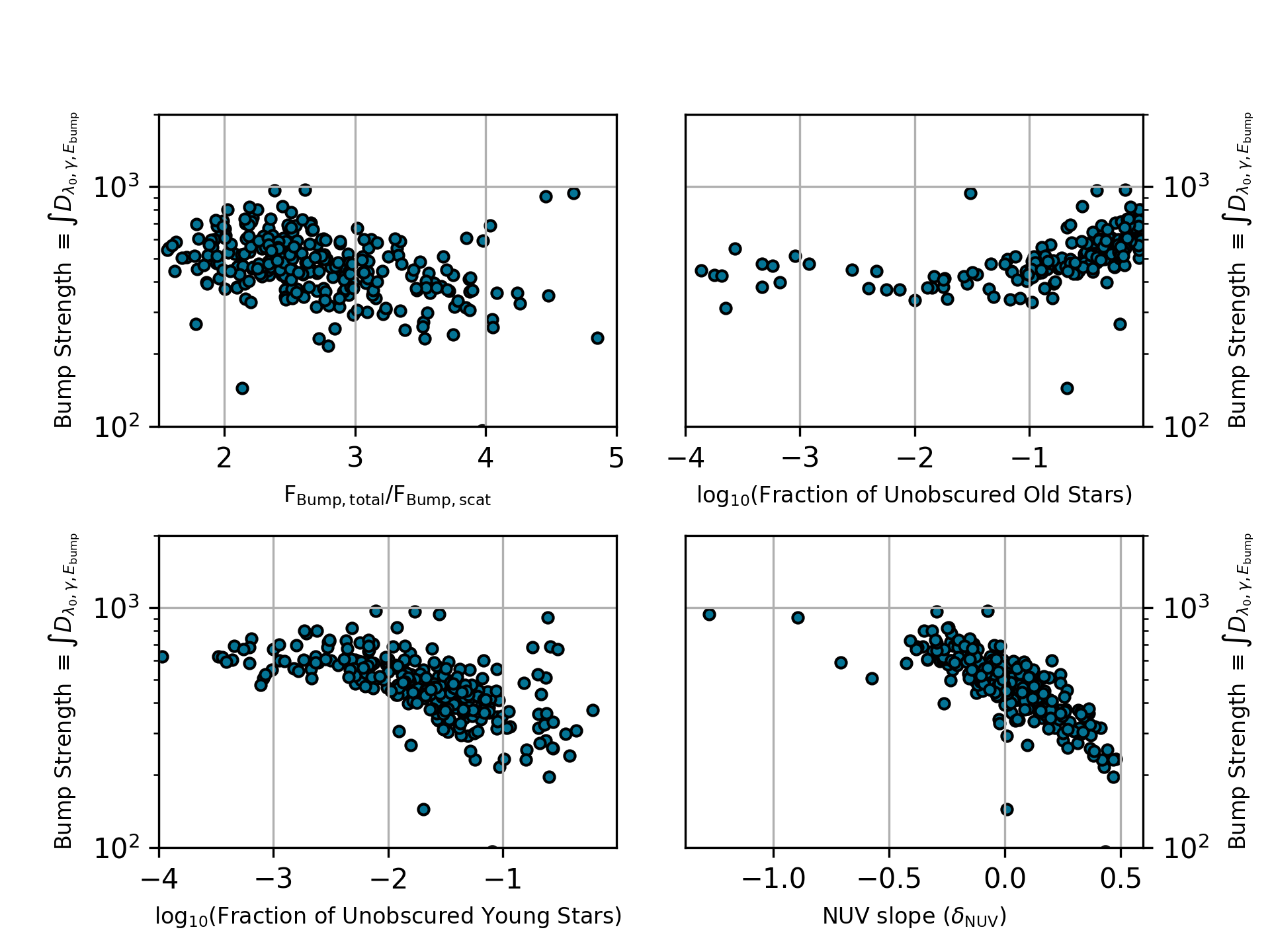
In Figure 8, we show how the bump strength varies in our models with a number of relevant quantities. The top left panel of Figure 8 shows the relationship between the UV bump strength and the fraction of scattered light contributing to the total flux. There is a relatively weak correlation between the two: light scattered into the line of sight contributes modestly to reduced bump strengths in some attenuation curves, but it clearly does not dominate.
In the top right and bottom left panels of Figure 8, we investigate the role of unobscured stars in contributing to reduced bump strengths. The top right panel shows the bump strengths as a function of the fraction of unobscured old ( Myr) stars, while the bottom left shows the bump strengths as a function of the fraction of unobscured young ( Myr) stars. As is clear, the old stars, which put out relatively little flux in the NUV, do not contribute significantly to filling in the absorption bump, even at relatively large unobscured fractions (and in fact trend in the opposite direction). In contrast, however, there is a clear relationship between the fraction of unobscured young stars, and the UV bump strength. In galaxies with increasingly complex young star-dust geometries, as more young stars find low- UV sightlines, this radiation fills in the UV bump and reduces its strength. In short: galaxies with very complex young star-dust geometries have reduced UV bumps.
Drawing on what we learned in § 4.3, the fraction of unobscured young stars in our simulations also correlates with the slope of the dust attenuation curve. It follows transitively, then, that the bump strength should vary inversely with the attenuation curve slope. We quantify this relationship in the bottom right panel of Figure 8, where we show the attenuation curve bump strength vs. NUV slope (; c.f. Equation 10). The greyest attenuation curves represent galaxies with the most complex young star-dust geometry, and therefore have the weakest bump strengths. While we will return to this issue further in § 5, but it’s worth briefly noting that Kriek & Conroy (2013) demonstrated that for galaxies in the NEWFIRM survey, dust attenuation slope varies inversely with the measured bump strength. This may provide some tentative evidence for our interpretation.
|
5 Discussion
5.1 Does a Single Attenuation Prescription Apply?
Thus far, we have explored the physical underpinnings of variations in dust attenuation curves in galaxies. We now ask the slightly more practical question: what range of attenuation curves can one expect for galaxies at a given redshift?
To answer this, we employ the Mpc3 mufasa cosmological hydrodynamic galaxy formation simulation (Davé et al., 2016). This simulation has identical physics as our zoom models, save for the inclusion of the standard mufasa heuristic quenching model. The simulation is run with particles, but in a volume half the size of the one our zooms are selected from, resulting in an effective mass resolution a factor worse (i.e. larger particle masses) than our zoom models. Achieving the full resolution of our zoom simulations in a cosmological volume requires a computational effort outside the scope of the current investigation.
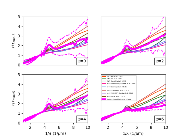
In Figures 9 and 10, we show heat maps of the attenuation curves for all galaxies555With caesar, we identify galaxies as FOF groups with at least star particles. This corresponds to a minimum stellar mass of . in the Mpc3 volume at redshifts . We additionally show the median attenuation curve (computed by calculating the median at every wavelength ) at each redshift via the solid pink line, and the standard deviation in the dashed pink lines. In order to best compare with observations which typically only select star-forming galaxies, we restrict our analysis here to galaxies with SFR yr-1. Figure 9 shows the heat map and median attenuation curves, and Figure 10 shows the median curves in comparison to literature references.
At each redshift, there is significant dispersion about the median, as evidenced by the heat map. In the normalized attenuation curves, a wide range of curve tilts and bump strengths are exhibited. The significant dispersion seen in Figure 9 is expected from observational constraints that show a diverse range of slopes in attenuation curves (e.g. Wild et al., 2011; Battisti et al., 2017). This dispersion in curves decreases with increasing redshift. While galaxy geometry remains complex at these epochs, the metal content (and hence, manifestly in these simulations, dust content) decreases, thus reducing the impact of star-dust geometry on the attenuation curve shape. Beyond this, there is a much narrower distribution in median stellar ages with increasing redshift (c.f. § 4.3).
Despite the strong dispersion seen at nearly all redshifts, the medians in the broad distribution of modeled attenuation curves are always bounded by the standard literature attenuation curves. This is demonstrated in Figure 9, where we compare against standard literature curves. For convenience, we have published the best fitting median curves in Figure 9 at integer redshifts from on a publicly accessible website666https://bitbucket.org/desika/narayanan_attenuation_laws/. It is important to note that while the median values are appropriate for ensemble averages, these median values (or any assumption of a locally-calibrated curve, for that matter) may grossly mischaracterize the underlying attenuation on a case by case basis.
Finally, it is worth noting that the most common attenuation curves in any of our modeled redshift bins all have prominent bump features. It is indeed possible to generate attenuation curves with relatively small bump contributions: this is demonstrated explicitly in Figures 6 and 8. These curves with minimal bumps owe their origin solely to geometry and radiative transfer effects (i.e. no modification of the underlying dust properties is necessary). This said, this is not typical in our models: the median curve within any redshift bin in Figure 9 displays a prominent bump.

|
|
5.2 Comparison to Other Models and Constraints
To our knowledge, this paper represents the first cosmological hydrodynamic simulation of galaxy formation investigating theoretical dust attenuation curves in galaxies. This said, our work builds on a deep theoretical literature. In this section, we aim to place the results from our work in this context. We painted the landscape for theoretical work in this field in § 1. In this section, we aggregate some key results from these papers, and compare them to our own investigation.
5.2.1 On the Role of Geometry
In Figures 3, and 7, we demonstrated via both population synthesis experiments as well as direct cosmological simulation that the role of the star-dust geometry is paramount in driving the tilt of normalized attenuation curves. For young galaxies, an increasing fraction of unobscured young stars flattens normalized attenuation curves, while for galaxies dominated by older stellar populations, an increasing fraction of unobscured old stars steepens normalized curves.
In general, at least the former point (and more broadly, the idea that geometry plays an important role in setting the shape of attenuation curves), is already well-appreciated in the theoretical literature. Indeed, a broad range of modeling techniques arrive at the same conclusion. For example, Witt & Gordon (1996) examined radiative transfer models in a two-phase clumpy medium, and found that as a general rule, attenuation curves became greyer (flatter) as the obscuration inhomogeneity increased. Seon & Draine (2016) expanded upon these results by using a turbulent studying the radiative transfer in a turbulent medium, and arrived at a similar conclusion, while Natale et al. (2015) utilized a coupling of 3D dust radiative transfer calculations (as in this paper) with idealized hydrodynamic models of disks in evolution to demonstrate this principle. Fischera & Dopita (2011) additionally employed non-homogeneous ISM models to explain grey attenuation curves.
It is important to note that the concept of increased complexity in the star-dust geometry driving greyer attenuation curves only applies to galaxies whose light are dominated by young stellar populations (c.f. Figure 7). In our model, galaxies whose luminosity is dominated by older stellar populations have normalized attenuation curves that become steeper as more old stars are decoupled from dust.
5.2.2 Bump Strengths
When assuming an attenuation curve for the purposes of SED fitting in low-metallicity galaxies (especially at high-redshift), a common assumption is an SMC-like attenuation curve. This is motivated by the assumption that the bumpless curve from the SMC may owe its origin to different grain compositions (presumably driven by the galaxy’s low metallicity) than in the Milky Way. Similar logic oftentimes motivate the usage of a bumpless Calzetti et al. (2000) curve to observations of heavily star-forming galaxies.
Throughout this work, we have demonstrated that even without changing the underlying grain properties (i.e., our extinction curve in every model is identical), we are able to generate extinction curves that have a diverse range in bump strengths (see, e.g. Figure 9 for one such example). In other words, curves with very small bump strengths in our models result simply from the geometry of the system. This conclusion is not necessarily shared amongst other theoretical models.
For example, Witt & Gordon (2000) expanded on the radiative transfer models of Witt & Gordon (1996), and found that they required a change to the intrinsic dust curve in order to make a bumpless curve. In specific, only by employing an extinction curve without a bump were they able to reproduce observed bump-free curves. Others (e.g. Fischera & Dopita, 2011) have suggested models in which the UV bump carriers are destroyed at threshold column densities in order to reproduce the Calzetti et al. (2000) curve.
Hou et al. (2017) implemented a full dust formation and destruction model into cosmological hydrodynamic simulations, and track the grain size distribution and extinction curve. While they do not model the radiative transfer associated with these simulations, they find in the extinction curve that bump strengths are naturally correlated with dust growth dominated by accretion of metals onto dust grains. While this study does not explore the geometry effects that drive attenuation curves, it is certainly conceivable that intrinsic dust properties can impact the strength of the UV bump.
At the same time, other models have suggested, like this work, that it may be possible to achieve bump-free attenuation curves without modifying the underlying extinction curve. For example, Granato et al. (2000) developed semi-analytic models to demonstrate that the bump-free Calzetti et al. (2000) curve may be a result of a ’birth cloud’ model, wherein the radiation from young stars are heavily attenuated by their birth clouds, but older stars are only attenuated by diffuse ISM. In this picture, the observed UV is dominated by an older stellar population which sees relatively little diffuse dust, and hence the emission from these objects can fill in the absorption feature. This semi-analytic model was expanded upon by Panuzzo et al. (2007), who found similar results.
While the Granato et al. (2000) and Panuzzo et al. (2007) studies share in common with our model the idea that an attenuation curve with very small bump strengths is achievable without changing the underlying extinction properties of grains, the models share a key difference. Granato et al. (2000) and Panuzzo et al. (2007) find that as young stellar populations become more obscured, bump sizes decrease in attenuation curves. In contrast, in Figure 8, we demonstrate that the opposite is true for our models: as a larger fraction of young stars becomes unobscured, observed bump strengths decrease owing to the UV radiation from these young stars filling in the absorption feature. An important corollary to our model is that the same displacement between O and B stars and sites of dust obscuration result in greyer (flatter) attenuation curves, leading to a natural relationship where shallower attenuation curves have smaller bump features in our model (bottom right panel of Figure 8).
Seon & Draine (2016) similarly derived a model for dust attenuation curves that exhibits a relationship between bump strength and slope of the attenuation curve in the same direction as both our models, and the Kriek & Conroy (2013) observations. This too can be attributed to geometry effects, wherein as the clumping or size of the source distribution increase, attenuation curves become greyer and exhibit smaller bumps. We note, however, that a Calzetti et al. (2000) curve is only attainable using the Weingartner & Draine (2001) Milky Way dust model when the intrinsic bump is removed or suppressed in the Seon & Draine (2016) model. As a result, their model may be viewed as intermediate between the results of Granato et al. (2000); Panuzzo et al. (2007) and ours.

|
5.3 Comparison with Observations
We now turn to a comparison of our models with relatively recent observational results in this area. We remind the reader of the discussion surrounding Equations 16-17 and Table 2. In specific, while we find a piece-wise fit to provide the best fits to our model attenuation curves as outlined in § 4.2, many observational studies employ a modified Calzetti et al. (2000) relation, where both a Drude-like profile for the UV bump as well as a power-law modification are employed (e.g. Noll et al., 2009). As we clarify in Table 2, we distinguish the power-law index derived from this method of fitting () from the power-law we typically employ just in the NUV bands ().
We compare to the observational results of Kriek & Conroy (2013), Salmon et al. (2016) and Salim et al. (2018) in Figure 11. Salmon et al. (2016) and Salim et al. (2018) derive attenuation laws for redshift and galaxies, respectively, via SED fitting techniques. Evident from both of these studies is a relationship between the -band optical depth and the slope of the attenuation curve, . This is similar to the powerlaw relationship modeled by Chevallard et al. (2013) and Leja et al. (2017) between the optical depth of diffuse dust and the powerlaw slope of the attenuation curve. In the left panel of Figure 11, we show a comparison between our models and this observed trend. We include every galaxy in our sample of zooms, though note that the Salmon et al. (2016) study and Salim et al. (2018) study of course both employ individual selection techniques within particular redshift ranges. Given both this, as well as the relative uncertainties involved in deriving attenuation curves from SED fitting, the trend of increasing with -band optical depth in the model galaxies is encouraging.
Kriek & Conroy (2013) employed SED fitting techniques to observations of galaxies to derive a relationship between the UV bump strength and slope power-law index, . In Figure 8, we demonstrated a similar relationship, though characterized this in terms of the integrated Drude profile, , and the NUV slope, . Kriek & Conroy (2013) fix the width of the bump to , and therefore characterize the strength of the bump by its normalization, (c.f. Table 2). In order to best compare to this study, we have re-performed our fits by fixing our bump widths similarly, and report in the right side of Figure 11 our modeled relationship between and . We show our model points in blue, and compare these to the Kriek & Conroy (2013) data in orange. The best fit lines for both are shown. Our model galaxies show a similar trend as the Kriek & Conroy (2013) observations in that steeper curves tend to have more prominent bump strengths. In our model, this owes primarily to unobscured young stars reducing bump strengths. Our modeled best fit relation is:
| (19) |
Our model galaxies exhibit a much shallower gradient than what is observed. This may owe to a number of causes. First, our modeled bump widths, (c.f. Equation 10) span a broad range of values, with some widths exceeding twice the assumed employed for the construction of Figure 11. Forcing a bump strength, therefore, may result in poorly performing fits, and therefore values that do not reflect the true dynamic range of bump strengths. As an example, examination of the bottom right panel of Figure 8 demonstrates that when considering the integral of the Drude profile of the bump strength, we see a dynamic range spanning an order of magnitude in bump strength, unlike the factor when characterizing the bump strength by alone. Beyond this, a true apples-to-apples comparison between our model points and the observed data would involve our fitting our model SEDs (assuming a given star formation history and IMF), and recovering the inferred attenuation law accordingly. Exploring the differences resulting in inferred attenuation curves from SED modeling from those directly modeled will be presented in future work. We note that Seon & Draine (2016) derived relationships between and that were typically steeper than the Kriek & Conroy (2013) relation. More observational and theoretical work in this area is warranted.
6 Conclusions and Summary
We have developed a model for the origin of variations in dust attenuation curve shapes and bump strengths. We accomplish this by combining high-resolution cosmological galaxy formation simulations with 3D dust radiative transfer calculations. Critically, for these radiative transfer models, we hold the underlying extinction curve fixed, and ask how geometry and radiative transfer effects impact the resultant attenuation curves. Our main results follow:
-
1.
Despite the usage of a constant extinction curve in our underlying radiative transfer calculations, we find dramatic variations in the derived attenuation laws. These variations depend primarily on complexities in the star-dust geometry (Figures 3, 6, & 7). In detail:
- (a)
- (b)
-
(c)
These results taken together drive a trend where galaxies with highly obscured sightlines toward young stars, but a significant (unobscured) evolved stellar population will have the steepest normalized attenuation curves (Figure 7).
-
2.
The UV bump strengths vary dramatically, despite our usage of an extinction curve with a UV bump present. Unobscured O and B stars result in reduced bump strengths in our model, with scattered light only having a secondary effect on the feature (Figure 8).
-
3.
The combined effect of unobscured young stars both flattening attenuation curve slopes, as well as reducing the bump strength results in a natural relationship wherein the slope of the attenuation curve is related to the bump strength: flatter attenuation curves tend to have smaller bump strengths (Figure 8).
-
4.
We apply these results to a Mpc/h cosmological volume to derive the median curve and expected dispersion at integer redshifts from . While the median curve at a given redshift is typically bounded by standard literature curves, the dispersion is significant. The average dispersion decreases with increasing redshift, and the median curves become greyer. This owes to reduced dispersion in star-dust geometry, as well as narrower distribution in median stellar ages with redshift (Figure 9). We publish these median curves on a public-facing website.
Acknowledgements
D.N. is grateful to Andrew Battisti, Daniela Calzetti, Rob Kennicutt, Maciej Koprowski, Karin Sandstrom, Samir Salim, Brett Salmon and George Privon for valuable conversations during this study. We additionally thank Mariska Kriek, Samir Salim and Brett Salmon for providing data to us for our comparisons with observations. The simulations published here were run on the University of Florida HiPerGator supercomputing facility, and the authors acknowledge the University of Florida Research Computing for providing computational resources and support that have contributed to the research results reported in this publication. This study was funded in part by NSF AST-1715206 and HST AR-15043.0001.
References
- Abruzzo et al. (2018) Abruzzo M. W., Narayanan D., Davé R., Thompson R., 2018, arXiv/1803.02374,
- Battisti et al. (2016) Battisti A. J., Calzetti D., Chary R.-R., 2016, ApJ, 818, 13
- Battisti et al. (2017) Battisti A. J., Calzetti D., Chary R.-R., 2017, ApJ, 840, 109
- Bell et al. (2002) Bell E. F., Gordon K. D., Kennicutt Jr. R. C., Zaritsky D., 2002, ApJ, 565, 994
- Böker et al. (1999) Böker T., et al., 1999, ApJS, 124, 95
- Bourne et al. (2016) Bourne N., et al., 2016, arXiv/1607.04283,
- Bruzual & Charlot (2003) Bruzual G., Charlot S., 2003, MNRAS, 344, 1000
- Buat et al. (2011) Buat V., Giovannoli E., Takeuchi T. T., Heinis S., Yuan F.-T., Burgarella D., Noll S., Iglesias-Páramo J., 2011, A&A, 529, A22
- Burgarella et al. (2005) Burgarella D., Buat V., Iglesias-Páramo J., 2005, MNRAS, 360, 1413
- Calzetti (1997) Calzetti D., 1997, AJ, 113, 162
- Calzetti (2001) Calzetti D., 2001, PASP, 113, 1449
- Calzetti et al. (1994) Calzetti D., Kinney A. L., Storchi-Bergmann T., 1994, ApJ, 429, 582
- Calzetti et al. (2000) Calzetti D., Armus L., Bohlin R. C., Kinney A. L., Koornneef J., Storchi-Bergmann T., 2000, ApJ, 533, 682
- Cardelli et al. (1989) Cardelli J. A., Clayton G. C., Mathis J. S., 1989, ApJ, 345, 245
- Casey et al. (2014a) Casey C. M., Narayanan D., Cooray A., 2014a, Physics Reports, 541, 45
- Casey et al. (2014b) Casey C. M., et al., 2014b, ApJ, 796, 95
- Chabrier (2003) Chabrier G., 2003, PASP, 115, 763
- Charlot & Fall (2000) Charlot S., Fall S. M., 2000, ApJ, 539, 718
- Chevallard et al. (2013) Chevallard J., Charlot S., Wandelt B., Wild V., 2013, MNRAS, 432, 2061
- Clayton et al. (2015) Clayton G. C., Gordon K. D., Bianchi L. C., Massa D. L., Fitzpatrick E. L., Bohlin R. C., Wolff M. J., 2015, ApJ, 815, 14
- Conroy (2010) Conroy C., 2010, MNRAS, 404, 247
- Conroy (2013) Conroy C., 2013, ARA&A, 51, 393
- Conroy & Gunn (2010) Conroy C., Gunn J. E., 2010, ApJ, 712, 833
- Conroy et al. (2009) Conroy C., Gunn J. E., White M., 2009, ApJ, 699, 486
- Conroy et al. (2010a) Conroy C., White M., Gunn J. E., 2010a, ApJ, 708, 58
- Conroy et al. (2010b) Conroy C., Schiminovich D., Blanton M. R., 2010b, ApJ, 718, 184
- Cullen et al. (2017a) Cullen F., et al., 2017a, arXiv/1712.01292,
- Cullen et al. (2017b) Cullen F., McLure R. J., Khochfar S., Dunlop J. S., Dalla Vecchia C., 2017b, MNRAS, 470, 3006
- Dalcanton et al. (2015) Dalcanton J. J., et al., 2015, ApJ, 814, 3
- Davé et al. (2011) Davé R., Finlator K., Oppenheimer B. D., 2011, arXiv/1108.0426,
- Davé et al. (2016) Davé R., Thompson R., Hopkins P. F., 2016, MNRAS, 462, 3265
- Davé et al. (2017a) Davé R., Rafieferantsoa M. H., Thompson R. J., Hopkins P. F., 2017a, MNRAS,
- Davé et al. (2017b) Davé R., Rafieferantsoa M. H., Thompson R. J., 2017b, arXiv/1704.01335,
- Draine (2003) Draine B. T., 2003, ARA&A, 41, 241
- Draine & Li (2007) Draine B. T., Li A., 2007, ApJ, 657, 810
- Draine & Malhotra (1993) Draine B. T., Malhotra S., 1993, ApJ, 414, 632
- Dwek (1998) Dwek E., 1998, ApJ, 501, 643
- Elíasdóttir et al. (2009) Elíasdóttir Á., et al., 2009, ApJ, 697, 1725
- Fischera & Dopita (2011) Fischera J., Dopita M., 2011, A&A, 533, A117
- Fitzpatrick (1999) Fitzpatrick E. L., 1999, PASP, 111, 63
- Fitzpatrick & Massa (1990) Fitzpatrick E. L., Massa D., 1990, ApJS, 72, 163
- Fitzpatrick & Massa (2007) Fitzpatrick E. L., Massa D., 2007, ApJ, 663, 320
- Fontanot & Somerville (2011) Fontanot F., Somerville R. S., 2011, MNRAS, 416, 2962
- Fontanot et al. (2009) Fontanot F., Somerville R. S., Silva L., Monaco P., Skibba R., 2009, MNRAS, 392, 553
- Galliano et al. (2017) Galliano F., Galametz M., Jones A. P., 2017, preprint, (arXiv:1711.07434)
- Geach et al. (2016) Geach J. E., et al., 2016, arXiv/1608.02941,
- Gonzalez-Perez et al. (2013) Gonzalez-Perez V., Lacey C. G., Baugh C. M., Frenk C. S., Wilkins S. M., 2013, MNRAS, 429, 1609
- Gordon et al. (1999) Gordon K. D., Smith T. L., Clayton G. C., 1999, in Bunker A. J., van Breugel W. J. M., eds, Astronomical Society of the Pacific Conference Series Vol. 193, The Hy-Redshift Universe: Galaxy Formation and Evolution at High Redshift. p. 517
- Gordon et al. (2000) Gordon K. D., Clayton G. C., Witt A. N., Misselt K. A., 2000, ApJ, 533, 236
- Gordon et al. (2003) Gordon K. D., Clayton G. C., Misselt K. A., Landolt A. U., Wolff M. J., 2003, ApJ, 594, 279
- Granato et al. (2000) Granato G. L., Lacey C. G., Silva L., Bressan A., Baugh C. M., Cole S., Frenk C. S., 2000, ApJ, 542, 710
- Grasha et al. (2013) Grasha K., Calzetti D., Andrews J. E., Lee J. C., Dale D. A., 2013, ApJ, 773, 174
- Hahn & Abel (2011) Hahn O., Abel T., 2011, MNRAS, 415, 2101
- Hayward & Smith (2015) Hayward C. C., Smith D. J. B., 2015, MNRAS, 446, 1512
- Hayward et al. (2013) Hayward C. C., Narayanan D., Kereš D., Jonsson P., Hopkins P. F., Cox T. J., Hernquist L., 2013, MNRAS, 428, 2529
- Heinis et al. (2013) Heinis S., et al., 2013, MNRAS, 429, 1113
- Hopkins (2015) Hopkins P. F., 2015, MNRAS, 450, 53
- Hopkins (2017) Hopkins P. F., 2017, arXiv/1712.01294,
- Hopkins et al. (2013) Hopkins P. F., Narayanan D., Murray N., Quataert E., 2013, MNRAS, 433, 69
- Hopkins et al. (2014) Hopkins P. F., Kereš D., Oñorbe J., Faucher-Giguère C.-A., Quataert E., Murray N., Bullock J. S., 2014, MNRAS, 445, 581
- Hopkins et al. (2017) Hopkins P. F., et al., 2017, arXiv/1702.06148,
- Hou et al. (2017) Hou K.-C., Hirashita H., Nagamine K., Aoyama S., Shimizu I., 2017, MNRAS, 469, 870
- Hoyle & Wickramasinghe (1962) Hoyle F., Wickramasinghe N. C., 1962, MNRAS, 124, 417
- Iwamoto et al. (1999) Iwamoto K., Brachwitz F., Nomoto K., Kishimoto N., Umeda H., Hix W. R., Thielemann F.-K., 1999, ApJS, 125, 439
- Johnson et al. (2007a) Johnson B. D., et al., 2007a, ApJS, 173, 377
- Johnson et al. (2007b) Johnson B. D., et al., 2007b, ApJS, 173, 392
- Jonsson (2006) Jonsson P., 2006, MNRAS, 372, 2
- Kennicutt (1998) Kennicutt Jr. R. C., 1998, ARA&A, 36, 189
- Kennicutt & Evans (2012) Kennicutt R. C., Evans N. J., 2012, ARA&A, 50, 531
- Kinney et al. (1994) Kinney A. L., Calzetti D., Bica E., Storchi-Bergmann T., 1994, ApJ, 429, 172
- Kong et al. (2004) Kong X., Charlot S., Brinchmann J., Fall S. M., 2004, MNRAS, 349, 769
- Koprowski et al. (2016) Koprowski M. P., et al., 2016, ApJ, 828, L21
- Kriek & Conroy (2013) Kriek M., Conroy C., 2013, ApJ, 775, L16
- Kroupa (2002) Kroupa P., 2002, Science, 295, 82
- Krumholz et al. (2009) Krumholz M. R., McKee C. F., Tumlinson J., 2009, ApJ, 693, 216
- Leja et al. (2017) Leja J., Johnson B. D., Conroy C., van Dokkum P. G., Byler N., 2017, ApJ, 837, 170
- Lo Faro et al. (2017) Lo Faro B., Buat V., Roehlly Y., Alvarez-Marquez J., Burgarella D., Silva L., Efstathiou A., 2017, MNRAS, 472, 1372
- Lucy (1999) Lucy L. B., 1999, A&A, 344, 282
- Marigo & Girardi (2007) Marigo P., Girardi L., 2007, A&A, 469, 239
- Marigo et al. (2008) Marigo P., Girardi L., Bressan A., Groenewegen M. A. T., Silva L., Granato G. L., 2008, A&A, 482, 883
- McKinnon et al. (2016) McKinnon R., Torrey P., Vogelsberger M., 2016, MNRAS, 457, 3775
- McLure et al. (2017) McLure R. J., et al., 2017, arXiv/1709.06102,
- Meurer et al. (1999) Meurer G. R., Heckman T. M., Calzetti D., 1999, ApJ, 521, 64
- Misselt et al. (1999) Misselt K. A., Clayton G. C., Gordon K. D., 1999, ApJ, 515, 128
- Motta et al. (2002) Motta V., et al., 2002, ApJ, 574, 719
- Muratov et al. (2015) Muratov A. L., Kereš D., Faucher-Giguère C.-A., Hopkins P. F., Quataert E., Murray N., 2015, MNRAS, 454, 2691
- Narayanan et al. (2008) Narayanan D., Cox T. J., Shirley Y., Davé R., Hernquist L., Walker C. K., 2008, ApJ, 684, 996
- Narayanan et al. (2009) Narayanan D., Cox T. J., Hayward C. C., Younger J. D., Hernquist L., 2009, MNRAS, 400, 1919
- Narayanan et al. (2010) Narayanan D., Hayward C. C., Cox T. J., Hernquist L., Jonsson P., Younger J. D., Groves B., 2010, MNRAS, 401, 1613
- Narayanan et al. (2012) Narayanan D., Krumholz M. R., Ostriker E. C., Hernquist L., 2012, MNRAS, 421, 3127
- Narayanan et al. (2015) Narayanan D., et al., 2015, Nature, 525, 496
- Narayanan et al. (2018) Narayanan D., Davé R., Johnson B. D., Thompson R., Conroy C., Geach J., 2018, MNRAS, 474, 1718
- Natale et al. (2015) Natale G., Popescu C. C., Tuffs R. J., Debattista V. P., Fischera J., Grootes M. W., 2015, MNRAS, 449, 243
- Noll et al. (2007) Noll S., Pierini D., Pannella M., Savaglio S., 2007, A&A, 472, 455
- Noll et al. (2009) Noll S., Burgarella D., Giovannoli E., Buat V., Marcillac D., Muñoz-Mateos J. C., 2009, A&A, 507, 1793
- Nomoto et al. (2006) Nomoto K., Tominaga N., Umeda H., Kobayashi C., Maeda K., 2006, Nuclear Physics A, 777, 424
- Olsen et al. (2017) Olsen K., Greve T. R., Narayanan D., Thompson R., Davé R., Niebla Rios L., Stawinski S., 2017, ApJ, 846, 105
- Oppenheimer & Davé (2008) Oppenheimer B. D., Davé R., 2008, MNRAS, 387, 577
- Pannella et al. (2009) Pannella M., et al., 2009, ApJ, 698, L116
- Panuzzo et al. (2007) Panuzzo P., Granato G. L., Buat V., Inoue A. K., Silva L., Iglesias-Páramo J., Bressan A., 2007, MNRAS, 375, 640
- Papovich et al. (2001) Papovich C., Dickinson M., Ferguson H. C., 2001, ApJ, 559, 620
- Pei (1992) Pei Y. C., 1992, ApJ, 395, 130
- Popescu et al. (2011) Popescu C. C., Tuffs R. J., Dopita M. A., Fischera J., Kylafis N. D., Madore B. F., 2011, A&A, 527, A109
- Popping et al. (2017a) Popping G., Somerville R. S., Galametz M., 2017a, MNRAS, 471, 3152
- Popping et al. (2017b) Popping G., Puglisi A., Norman C. A., 2017b, MNRAS, 472, 2315
- Privon et al. (2018) Privon G. C., Narayanan D., Davé R., 2018, arXiv/1805.03469,
- Reddy & Steidel (2004) Reddy N. A., Steidel C. C., 2004, ApJ, 603, L13
- Reddy et al. (2008) Reddy N. A., Steidel C. C., Pettini M., Adelberger K. L., Shapley A. E., Erb D. K., Dickinson M., 2008, ApJS, 175, 48
- Reddy et al. (2012) Reddy N., et al., 2012, ApJ, 744, 154
- Reddy et al. (2015) Reddy N. A., et al., 2015, ApJ, 806, 259
- Rieke & Lebofsky (1985) Rieke G. H., Lebofsky M. J., 1985, ApJ, 288, 618
- Robitaille (2011) Robitaille T. P., 2011, A&A, 536, A79
- Rocha et al. (2008) Rocha M., Jonsson P., Primack J. R., Cox T. J., 2008, MNRAS, 383, 1281
- Safarzadeh et al. (2017) Safarzadeh M., Hayward C. C., Ferguson H. C., 2017, ApJ, 840, 15
- Salim et al. (2007) Salim S., et al., 2007, ApJS, 173, 267
- Salim et al. (2018) Salim S., Boquien M., Lee J. C., 2018, arXiv/1804.05850,
- Salmon et al. (2016) Salmon B., et al., 2016, ApJ, 827, 20
- Schmidt (1959) Schmidt M., 1959, ApJ, 129, 243
- Scoville et al. (2015) Scoville N., Faisst A., Capak P., Kakazu Y., Li G., Steinhardt C., 2015, ApJ, 800, 108
- Seibert et al. (2002) Seibert M., Heckman T. M., Meurer G. R., 2002, AJ, 124, 46
- Seon & Draine (2016) Seon K.-I., Draine B. T., 2016, ApJ, 833, 201
- Shivaei et al. (2015) Shivaei I., Reddy N. A., Steidel C. C., Shapley A. E., 2015, ApJ, 804, 149
- Siana et al. (2009) Siana B., et al., 2009, ApJ, 698, 1273
- Springel et al. (2005) Springel V., Di Matteo T., Hernquist L., 2005, MNRAS, 361, 776
- Stecher (1965) Stecher T. P., 1965, ApJ, 142, 1683
- Stecher & Donn (1965) Stecher T. P., Donn B., 1965, ApJ, 142, 1681
- Stratta et al. (2007) Stratta G., Maiolino R., Fiore F., D’Elia V., 2007, ApJ, 661, L9
- Thompson (2014) Thompson R., 2014, pyGadgetReader: GADGET snapshot reader for python, Astrophysics Source Code Library (ascl:1411.001)
- Thompson et al. (2014) Thompson R., Nagamine K., Jaacks J., Choi J.-H., 2014, ApJ, 780, 145
- To et al. (2014) To C.-H., Wang W.-H., Owen F. N., 2014, ApJ, 792, 139
- Turk et al. (2011) Turk M. J., Smith B. D., Oishi J. S., Skory S., Skillman S. W., Abel T., Norman M. L., 2011, ApJS, 192, 9
- Vladilo (1998) Vladilo G., 1998, ApJ, 493, 583
- Wada et al. (1999) Wada S., Kaito C., Kimura S., Ono H., Tokunaga A. T., 1999, A&A, 345, 259
- Walcher et al. (2011) Walcher J., Groves B., Budavári T., Dale D., 2011, Ap&SS, 331, 1
- Watson (2011) Watson D., 2011, A&A, 533, A16
- Weingartner & Draine (2001) Weingartner J. C., Draine B. T., 2001, ApJ, 548, 296
- Welty & Fowler (1992) Welty D. E., Fowler J. R., 1992, ApJ, 393, 193
- Wild et al. (2011) Wild V., Charlot S., Brinchmann J., Heckman T., Vince O., Pacifici C., Chevallard J., 2011, MNRAS, 417, 1760
- Wilkins et al. (2012) Wilkins S. M., Gonzalez-Perez V., Lacey C. G., Baugh C. M., 2012, MNRAS, 424, 1522
- Witt & Gordon (1996) Witt A. N., Gordon K. D., 1996, ApJ, 463, 681
- Witt & Gordon (2000) Witt A. N., Gordon K. D., 2000, ApJ, 528, 799
- York et al. (2006) York D. G., et al., 2006, MNRAS, 367, 945