Optimal Scheduling and Exact Response Time Analysis for Multistage Jobs

Abstract.

Scheduling to minimize mean response time in an M/G/1 queue is a classic problem. The problem is usually addressed in one of two scenarios. In the perfect-information scenario, the scheduler knows each job’s exact size, or service requirement. In the zero-information scenario, the scheduler knows only each job’s size distribution. The well-known shortest remaining processing time (SRPT) policy is optimal in the perfect-information scenario, and the more complex Gittins policy is optimal in the zero-information scenario.

In real systems the scheduler often has partial but incomplete information about each job’s size. We introduce a new job model, that of multistage jobs, to capture this partial-information scenario. A multistage job consists of a sequence of stages, where both the sequence of stages and stage sizes are unknown, but the scheduler always knows which stage of a job is in progress. We give an optimal algorithm for scheduling multistage jobs in an M/G/1 queue and an exact response time analysis of our algorithm.

1. Introduction

Scheduling jobs to minimize mean response time in preemptive single-server queueing systems, such as the M/G/1 queue, has been the subject of countless papers over the past several decades. When the scheduler knows each job’s exact size, or service requirement, the shortest remaining processing time (SRPT) algorithm is optimal. When the scheduler does not know jobs’ sizes, the optimal policy is the Gittins policy [11; 2], which uses the job size distribution to give each job a priority based on its age, namely the amount of service the job has received so far. Although both SRPT and the Gittins policy have long been known to be optimal for their respective settings, only SRPT has been analyzed in the past [19]. There is no known closed form for mean response time under the Gittins policy.

In some sense, SRPT and the Gittins policy represent opposite extremes of optimal scheduling algorithms. SRPT treats the complete information case: we know each individual job’s exact size. The Gittins policy treats the zero information case: we have no information about individual jobs, leaving us only the overall size distribution and each job’s age on which to base a policy. This prompts a natural question: what policy is optimal in the partial information case, where we have nonzero but incomplete information about each job’s remaining size?

To model jobs with partial information about remaining size, we propose a new job model: multistage jobs. During service, a multistage job progresses through a sequence of stages, each of which has its own individual size, or service requirement. A job completes when its last stage completes. The sequence of stages a job goes through may be stochastic, and the server cannot influence the sequence of stages. Whereas a standard M/G/1 with unknown job sizes uses only the age of each job when scheduling, multistage jobs provide the scheduler both

• the current stage of the job and

• the age of the current stage.

Although stages may have general size distributions, stage sizes and transitions are Markovian in the sense that a job’s history before its current stage is independent of the sizes of and transitions between its current and future stages.

Jobs with multiple stages are so common in applications that it is surprising they have not received more attention. For instance, the following scenarios can be modeled with multistage jobs:

• At every moment in time, a Google ad server preemptively chooses which ad placement job to serve. Ad placement has three stages: preprocessing, which has uniform size distribution; targeting, which has bounded Pareto size distribution with a low bound; and selection, which has bounded Pareto size distribution with a high bound. Job  G in Figure 1.1 models an ad placement request as a multistage job.

• In a small general repair shop, a single repairer preemptively chooses which of multiple items to fix. Each item goes through two stages of service: diagnosis and repair. The amount of time repair takes depends on the problem with the item, which the repairer knows only after diagnosis. Job  R in Figure 1.1 models this repair process as a multistage job.

• Drugs are developed through multiple stages of research and trials. A single team preemptively chooses which of multiple drug projects to work on based on the state of each project.

Two examples of multistage jobs. Job  G is a Google ad placement request, which always goes through the same three stages before completion. The first stage, preprocessing, has uniform size distribution $P$. The other stages, targeting and selection, have bounded Pareto size distributions $T$ and $S$ with low and high upper bound, respectively. Job  R is a job in a general repair shop. The first stage is diagnosis, which takes time $D$. The other stages are repair work. With probability $p$, repair work is easy and takes time $R_{\text{easy}}$, and with probability $1-p$, repair work is hard and takes time $R_{\text{hard}}$.

Figure 1.1. Multistage Job Examples

To highlight the difference between multistage jobs and previous job models, consider multistage jobs A , B , and C in Figure 1.2. While all three jobs have total size distribution $S+2d$, where $S$ is stochastic and $d$ is deterministic, their stage structures make them very different.

• In job  A , the stochastic stage is after the deterministic stage: after serving A for time $2d$, we know the remaining size has distribution $S$.

• In job  B , the stochastic stage is before the deterministic stage: after serving B for a random amount of time $S$, we learn that the first stage has completed, at which point we know the remaining size is exactly $2d$.

• Job  C combines both of these effects: after serving C for time $d$, we then serve it for a random amount of time $S$ until we learn that the second stage has completed, at which point the remaining size is $d$.

Suppose we have a preemptive single-server system containing jobs A , B , and  C . Which job should we serve first to minimize mean response time? Is it better to serve A first to get the deterministic section out of the way? Is it better to serve B first, just in case we get lucky and its first stage finishes quickly? Is the compromise C a better or worse choice than each of the others?

How do we best exploit multistage structure when scheduling to minimize mean response time?

This is a difficult question to answer because it requires comparing not just jobs’ current size distributions but also their potential future size distributions. The differences between A , B , and C lie not in their initial size distributions, all $S+d$, but rather in how their size distributions might evolve with service. Adding to the difficulty is the fact that a multistage job’s remaining size distribution evolves stochastically, jumping every time a stage completes. This is more complicated than a single-stage job in the standard M/G/1, whose remaining size distribution depends only on its age. Jobs with stochastic stage sequences, such as job  R in Figure 1.1, exacerbate the difficulty.

Let $S$ be a stochastic size distribution and $d$ be a deterministic size. The three jobs A , B , and C all have the same total size distribution $S+2d$, but they have different stage structures.

Figure 1.2. Different Stage Structures for Same Total Size

To our knowledge, there is no prior theoretical work specifically pertaining to multistage jobs in a preemptive setting. Analyzing the mean response time of virtually any scheduling policy for multistage jobs is an open problem, let alone finding and analyzing the optimal policy. The closest prior work is Klimov’s model and variations [16; 25], which can model jobs with nonpreemptible stages, whereas our stages are preemptible. Nonpreemptible stages require far fewer scheduling decisions, which makes Klimov’s model simple to optimally schedule using a variant of the Gittins policy [5; 23; 11].

The main contribution of this paper is an optimal scheduling algorithm for multistage jobs. Thanks to a novel reduction technique, our algorithm is no more complex than optimally scheduling single-stage jobs. We exactly analyze the performance of our algorithm, obtaining a closed-form expression mean response time.

1.1. Background and Challenges

As mentioned above, we will reduce the problem of scheduling multistage jobs to the problem of scheduling single-stage jobs with unknown size, as in the standard M/G/1. It thus behooves us to review the single-stage setting, in which the Gittins policy minimizes mean response time [11; 2]. Remarkably, the Gittins policy has a very simple form: for each job, determine a quantity called its Gittins index, then serve the job of maximal Gittins index. While the Gittins policy has long been known to be optimal, its response time resisted analysis until recently, when Scully et al. [20] analyzed the class of SOAP policies, which includes the Gittins policy.

One might wonder whether we can apply the Gittins index to multistage jobs. The answer is yes, but with a caveat: it is possible to define the Gittins index of a multistage job, and the resulting Gittins policy minimizes mean response time, but computing a multistage job’s Gittins index requires solving a multidimensional optimization problem with one dimension per stage. This makes computing Gittins indices intractable. We might hope to tame this complexity by, for instance, computing the Gittins index of a multistage job by somehow combining the Gittins indices of its individual stages, which would allow us to leverage prior work on single-stage jobs, but there is no known way to do this.

Even if we could compute the Gittins policy for multistage jobs, analyzing its mean response time would still be challenging. The analysis of SOAP policies given by Scully et al. [20] is for single-stage jobs. While a similar method could in principle be used for multistage jobs, it would require considering all the possible sequences of stages, of which there can be exponentially many. No known analysis method scales gracefully to multistage jobs.

1.2. Contributions

In this paper, we solve the two main challenges outlined in Section 1.1: we give a simple method to compute the Gittins index of a multistage job, and we give a simple closed form for the mean response time of the Gittins policy for multistage jobs. Specifically, our contributions are as follows:

• We introduce multistage jobs, a new job model in which the scheduler has partial information about a job’s progress (Section 2).

• We introduce single-job profit (SJP), a new framework for the Gittins index that is especially well suited for multistage jobs (Section 3).

• Using the SJP framework, we state and prove a new composition law, which reduces a multistage job’s Gittins index computation into two smaller SJP computations which, unlike Gittins indices, naturally compose (Section 4). We give two applications of the composition law:

  • We show how repeated application of the composition law reduces any multistage job’s Gittins index computation to SJP computations for single-stage jobs (Section 4.1).

  • In special case of a fixed stage sequence with discrete size distributions, the problem simplifies considerably, and our composition law provides a divide-and-conquer algorithm for computing the Gittins index in $O(n\log n)$ time where $n$ is the total number of support points (Section 4.2).

• Using the SJP framework, we exactly analyze mean response time under our algorithm, giving a closed form in terms of SJP (Section 5).

• We give several practical takeaways for systems with multistage jobs (Section 6):

  • We demonstrate that, as a rough guideline, it is best to front-load stages with more variable length (Section 6.1). This answers the question posed by Figure 1.2.

  • We show that our algorithm significantly reduces response time compared to all algorithms that do not exploit multistage structure (Section 6.2).

Together, our contributions constitute the first theoretical analysis of multistage jobs with preemptible stages of general size distribution.

1.3. Related Work

The Gittins index has been extensively studied in the standard M/G/1 setting [2; 3; 17; 14], but there are few concrete results for more complex job models. A notable exception is Klimov’s model [16], which is a nonpreemptive multiclass M/G/1 queue with Bernoulli feedback: upon completion, jobs of class $i$ have some probability $p_{ij}$ of immediately returning as a class $j$ job. By thinking of classes as stages, we can think of a job in Klimov’s model as a job with multiple stages. One can optimally schedule Klimov’s model using the Gittins index [11, Section 4.9.2]. The fundamental difference between Klimov’s model and our model is that we allow preemption, which makes the space of possible policies much larger and makes Gittins index computation far more difficult. A variation of Klimov’s model studied by Whittle [25] allows preemption but requires each class’s size distribution to be exponential, whereas we study general size distributions.

The Gittins index has been applied to many problems in scheduling and beyond [11; 9; 12; 10; 22; 24; 8; 4; 25]. As such, there are many definitions of the Gittins index, all essentially equivalent but each with different strengths, such as providing intuition or enabling certain elegant proofs. SJP provides another definition of the Gittins index which is particularly well suited to working with multistage jobs. See Section 3.3 for a more detailed comparison between SJP and prior Gittins index formulations.

2. System Model

We consider the multistage M/G/1 queue, a preemptive single-server queueing system in which the jobs are multistage jobs. A multistage job goes through a stochastic sequence of stages during service. Each stage has a size, or service requirement.

In the multistage M/G/1, jobs arrive as a Poisson process of rate $\lambda$, and each job’s stage sizes and transitions are independent of those of other jobs and the arrival process. At every moment in time, the scheduler must decide which job to serve. The scheduler does not know jobs’ exact stage sequences or stages’ exact sizes ahead of time, but it does know the distributions of possible sequences and sizes (Section 2.1). Our goal is to minimize mean response time, the average time between a job’s arrival and completion. We assume a stable system, meaning the expected total size of each job is less than $1/\lambda$, and a preempt-resume model, meaning preemption and processor sharing are permitted with no penalty or loss of work.

2.1. Anatomy of a Multistage Job

In this section we zoom in on a single job and define its dynamics during service, summarizing the resulting notation in Table 2.1.

Every multistage job is a pair of two pieces of data: a type and a state. We can think of a job’s type as a “map” and a job’s state as a “location” on the map. As a job is served, it’s state evolves according to transition rules based on the job’s type. The scheduler knows the type and state of every job currently in the system.

A job type  J specifies the following information, which is all known to the scheduler.

• Type  J jobs have a finite set of possible stages, denoted $\mathcal{I}_{\texttt{\scalebox{1.04}{J}}}$. A stage is simply a label or name. Below we associate transition probabilities and a size distribution with each label.

• Each type  J job starts in the initial stage $a_{\texttt{\scalebox{1.04}{J}}}\in\mathcal{I}_{\texttt{\scalebox{1.04}{J}}}$.

• There is a special final stage $z_{\texttt{\scalebox{1.04}{J}}}\in\mathcal{I}_{\texttt{\scalebox{1.04}{J}}}$ that each type  J job enters upon completion.

• Upon completing stage $i$, a type  J job transitions to stage $j$ with transition probability $p^{\texttt{\scalebox{1.04}{J}}}_{ij}$. The stages form an acyclic Markov chain absorbing at $z_{\texttt{\scalebox{1.04}{J}}}$, meaning $z_{\texttt{\scalebox{1.04}{J}}}$ is accessible from all other stages and no stage is accessible from itself.

• Each stage $i\in\mathcal{I}_{\texttt{\scalebox{1.04}{J}}}$ has a size distribution $X_{i}$ representing the amount of service stage $i$ requires. We write $f_{i}$ and $\mkern 2.4mu\overline{\mkern-2.4muF\mkern-0.8mu}\mkern 0.8mu_{i}$ for the density and tail functions, respectively, of $X_{i}$. We always have $X_{z_{\texttt{\scalebox{1.04}{J}}}}=0$.

A job’s state, denoted $\langle i,x\rangle$, consists of the stage $i$ in progress and the age $x\geq 0$ of the stage, namely the amount of time the job has been served while in stage $i$. Stage transitions and stage sizes are independent, so the evolution of a job’s state $\langle i,x\rangle$ during service is Markovian, even for generally distributed stage sizes $X_{i}$. When a type  J job is served in state $\langle i,x\rangle$, the state experiences two kinds of transitions:

• The stage’s age $x$ increases continuously at rate $1$.

• The job’s state stochastically jumps from $\langle i,x\rangle$ to $\langle j,0\rangle$ at instantaneous rate $p^{\texttt{\scalebox{1.04}{J}}}_{ij}h_{i}(x)$, where

  $$h_{i}(x)=\frac{f_{i}(x)}{\mkern 2.4mu\overline{\mkern-2.4muF\mkern-0.8mu}\mkern 0.8mu_{i}(x)}$$

  is the hazard rate of stage size $X_{i}$ at age $x$.

A type  J job starts in state $\langle a_{\texttt{\scalebox{1.04}{J}}},0\rangle$ and completes, exiting the system, upon jumping to state $\langle z_{\texttt{\scalebox{1.04}{J}}},0\rangle$. We write $\mathbf{E}[X_{\texttt{\scalebox{1.04}{J}}}]$ for the expected total size of a type  J job, which is the expected amount of service time required for a type  J job to go from $\langle a_{\texttt{\scalebox{1.04}{J}}},0\rangle$ to $\langle z_{\texttt{\scalebox{1.04}{J}}},0\rangle$.

Table 2.1. Summary of Multistage Job Notation

Notation	Description
$\mathcal{I}_{\texttt{\scalebox{1.04}{J}}}$	set of possible stages of job type  J
$a_{\texttt{\scalebox{1.04}{J}}},z_{\texttt{\scalebox{1.04}{J}}}$	initial and final stages of job type  J
$p^{\texttt{\scalebox{1.04}{J}}}_{ij}$	transition probability from $i$ to $j$ in job type  J
$X_{i}$	size distribution of stage $i$
$\langle i,x\rangle$	state of a job at age $x$ of stage $i$
$f_{i},\mkern 2.4mu\overline{\mkern-2.4muF\mkern-0.8mu}\mkern 0.8mu_{i},h_{i}$	density, tail, and hazard rate functions of $X_{i}$
$\mathbf{E}[X_{\texttt{\scalebox{1.04}{J}}}]$	expected total size of  J
$\texttt{\scalebox{1.04}{J}}\langle i,x\rangle$	state-conditioned job type

2.2. Terminology Conventions

In Sections 3 and 4 we study single-job profit, a framework for computing the Gittins index of a multistage job. To simplify exposition, we assume that all jobs are in their initial state, and when we say “job  J ” we mean a type  J job in its initial state $\langle a_{\texttt{\scalebox{1.04}{J}}},0\rangle$. To apply our results to a job in any state, we can simply define a new job type. Specifically, given job type  J and state $\langle i,x\rangle$, the state-conditioned job type $\texttt{\scalebox{1.04}{J}}\langle i,x\rangle$ is the job type obtained by starting a type  J job in state $\langle i,x\rangle$. That is, a type $\texttt{\scalebox{1.04}{J}}\langle i,x\rangle$ job in state $\langle a_{\texttt{\scalebox{1.04}{J}}\langle i,x\rangle},0\rangle$ has future evolution stochastically equivalent to that of a type  J job in state $\langle i,x\rangle$. See Appendix A for a formal definition.

In Section 5 we study the M/G/1 with multistage jobs. To simplify notation, we assume that all jobs have the same job type  J and omit the J from the notation in Table 2.1. Despite using a single job type, we can model a system with multiple job classes with what we call a mixture composition (Definition 4.4): we give the initial stage $a$ size $X_{a}=0$, causing each new job to immediately transition to what we think of as the initial stage for its class.

3. Single-Job Profit: A New Framework for the Gittins Index

In this section we describe single-job profit (SJP), a new framework for defining and computing the Gittins index of a job. As we will see, SJP is particularly well suited to multistage jobs. We first define SJP (Section 3.1) then relate it to the Gittins index (Section 3.2). Throughout this section we define several terms and notations related to SJP, which we summarize in Table 3.1.

3.1. Definition of Single-Job Profit

We define single-job profit (SJP) to be an optimization problem concerning a single multistage job  J and a potential reward $r\geq 0$. At every moment in time, we must choose between one of two actions: serving and giving up. While serving, we incur cost at continuous rate $1$ as J ’s state evolves as described in Section 2.1. If J completes, we receive reward $r$ and the process ends. The other action, giving up, immediately ends the process with no additional cost or reward. Our goal is to maximize expected profit, meaning the expected reward received minus expected cost incurred.

Because J ’s state evolution is Markovian, to play optimally in SJP, it suffices to consider policies that decide to serve or give up based only on the current state. Thus, a policy for SJP is a stopping policy $\pi$ consisting of a stopping age $\pi(i)\geq 0$ for each stage $i$. A stopping policy $\pi$ gives up if J enters state $\langle i,\pi(i)\rangle$ for some stage $i$. For example, the policy of never giving up sets $\pi(i)=\infty$ for all stages $i$, and the policy of giving up immediately sets $\pi(a_{\texttt{\scalebox{1.04}{J}}})=0$.

Definition 3.1.

The optimal profit of job  J and reward $r$ in SJP is

$$V_{\texttt{\scalebox{1.04}{J}}}(r)=\sup_{\pi}(r\mathbf{P}\{\text{$\pi$ completes~{}$\texttt{\scalebox{1.04}{J}}$}\}-\mathbf{E}[\text{time $\pi$ serves~{}$\texttt{\scalebox{1.04}{J}}$}]),$$

where the supremum is taken over stopping policies $\pi$. The optimal profit as a function of reward $r$ is called J ’s SJP function.

It is intuitive that a state’s SJP function is nondecreasing, because a larger potential reward should not hurt the optimal profit. In fact, we can make a much stronger statement.

Lemma 3.2.

Every job’s SJP function $V_{\texttt{\scalebox{1.04}{J}}}(r)\kern-0.5pt$ is

1. convex and nondecreasing,

2. bounded above by $r\kern-0.5pt$,

3. bounded below by $\max\{0,r-\mathbf{E}[X_{\texttt{\scalebox{1.04}{J}}}]\}\kern-0.5pt$, and

4. differentiable almost everywhere with derivative at most $1\kern-0.5pt$.

Proof.

From Definition 3.1, we see $V_{\texttt{\scalebox{1.04}{J}}}(r)$ is a supremum of convex nondecreasing functions of $r$, implying claim i. No policy can receive reward greater than $r$ or incur cost less than $0$, implying claim ii. Possible policies for SJP include immediately giving up, which yields expected profit $0$, and never giving up, which yields expected profit $r-\mathbf{E}[X_{\texttt{\scalebox{1.04}{J}}}]$, implying claim iii. The conjunction of claims i and ii implies iv. ∎

By Lemma 3.2, J ’s SJP function has an inverse $V^{-1}_{\texttt{\scalebox{1.04}{J}}}(u)$ defined for all $u>0$. There are many possibilities for $V^{-1}_{\texttt{\scalebox{1.04}{J}}}(0)$. We choose the value that makes $V^{-1}_{\texttt{\scalebox{1.04}{J}}}(u)$ continuous at $u=0$, which is the largest possible value.

Definition 3.3.

The SJP index of job  J is

$$M_{\texttt{\scalebox{1.04}{J}}} =V^{-1}_{\texttt{\scalebox{1.04}{J}}}(0)$$

$$=\sup\{r\geq 0\mid V_{\texttt{\scalebox{1.04}{J}}}(r)=0\}$$

$$=\inf\{r\geq 0\mid V_{\texttt{\scalebox{1.04}{J}}}(r)>0\}.$$

Put another way, the SJP index of job  J is the smallest reward $r$ such that it is optimal to serve J for at least an instant in SJP. A state’s SJP index is a measure of how reluctant we are to serve a job in that state: the more reluctant we are to serve the job, the larger a reward we need to be offered to serve it.

Table 3.1. Summary of Single-Job Profit Notation

Notation	Description	Defined in
$V_{\texttt{\scalebox{1.04}{J}}}(r)$	SJP function of job  J	Definition 3.1
$M_{\texttt{\scalebox{1.04}{J}}}=V^{-1}_{\texttt{\scalebox{1.04}{J}}}(0)$	SJP index of job  J	Definition 3.3
$G_{\texttt{\scalebox{1.04}{J}}}=1/M_{\texttt{\scalebox{1.04}{J}}}$	Gittins index of job  J	Definition 3.4

3.2. Single-Job Profit and the Gittins Index

We now relate SJP to the traditional definition of the Gittins index, beginning with a review of the traditional definition.

The Gittins policy is a policy for minimizing mean response time in a variety of queueing systems, including the standard M/G/1 [2; 3] and the multistage M/G/1 considered herein. The policy has a simple form: always serve the job of maximal Gittins index. A job’s Gittins index, defined below, is unaffected by other jobs in the system.

Definition 3.4 ([11, Section 3.2]).

The Gittins index of job  J is

$$G_{\texttt{\scalebox{1.04}{J}}}=\sup_{\pi}\frac{\mathbf{P}\{\text{$\pi$ completes~{}$\texttt{\scalebox{1.04}{J}}$}\}}{\mathbf{E}[\text{time $\pi$ serves~{}$\texttt{\scalebox{1.04}{J}}$}]},$$

where the supremum is taken over stopping policies $\pi$ that do not immediately give up.

One interpretation of $G_{\texttt{\scalebox{1.04}{J}}}$ is as the maximum possible “completion rate” of  J : the numerator in Definition 3.4 is an expected number of job completions, and the denominator is the expected time for those completions to occur. The significance of Gittins indices lies in the following theorem.

Theorem 3.5 ([11, Corollary 3.5]).

The Gittins policy, which always serves the job of greatest Gittins index, minimizes mean response time in any single-server system with Poisson job arrivals and Markovian job dynamics.

The Gittins index theorem applies to our multistage M/G/1, but directly computing the Gittins indices of multistage job using Definition 3.4 requires optimizing the multidimensional parameter $\pi$. Fortunately, we can obtain a multistage job’s Gittins index from SJP as $G_{\texttt{\scalebox{1.04}{J}}}=1/M_{\texttt{\scalebox{1.04}{J}}}$. This helps because, as we show in Section 4.1, SJP with a multistage job reduces to several SJP instances with single-stage jobs.

Where does $G_{\texttt{\scalebox{1.04}{J}}}=1/M_{\texttt{\scalebox{1.04}{J}}}$ come from? Consider SJP with job  J and reward $r$ and ask: is it optimal to give up immediately? We can answer in two ways:

• Using the SJP index: By Definition 3.3, it is optimal to give up immediately if $r\leq M_{\texttt{\scalebox{1.04}{J}}}$.

• Using the Gittins index: Recall that we can think of $G_{\texttt{\scalebox{1.04}{J}}}$ as the maximum possible “completion rate” of  J . This means that with the right stopping policy, we can receive reward at average rate $rG_{\texttt{\scalebox{1.04}{J}}}$ while incurring cost at rate $1$, so it is optimal to give up immediately if $rG_{\texttt{\scalebox{1.04}{J}}}\leq 1$.

The following proposition formalizes this argument.

Proposition 3.6.

For any job  J ,

$$M_{\texttt{\scalebox{1.04}{J}}}=\frac{1}{G_{\texttt{\scalebox{1.04}{J}}}}.$$

Proof.

Throughout, $\pi$ ranges over stopping policies that do not give up immediately. Continuity ensures the supremum in Definition 3.1 is unchanged by omitting the policy of giving up immediately. Let

$$P_{\pi} =\mathbf{P}\{\text{$\pi$ completes~{}$\texttt{\scalebox{1.04}{J}}$}\}$$

$$E_{\pi} =\mathbf{E}[\text{time $\pi$ serves~{}$\texttt{\scalebox{1.04}{J}}$}].$$

We compute

$$M_{\texttt{\scalebox{1.04}{J}}}=\inf\{r\geq 0\mid V_{\texttt{\scalebox{1.04}{J}}}(r)>0\}=\inf\{r\geq 0\mid\sup_{\pi}(rP_{\pi}-E_{\pi})>0\}$$

and

$$\frac{1}{G_{\texttt{\scalebox{1.04}{J}}}}=\inf_{\pi}\frac{E_{\pi}}{P_{\pi}}=\inf\biggl{\{}r\geq 0\biggm{|}r>\inf_{\pi}\frac{E_{\pi}}{P_{\pi}}\biggr{\}}.$$

Each of $\sup_{\pi}(rP_{\pi}-E_{\pi})>0$ and $r>\inf_{\pi}E_{\pi}/P_{\pi}$ holds if and only if there exists a stopping policy $\pi$ such that $rP_{\pi}>E_{\pi}$, so $M_{\texttt{\scalebox{1.04}{J}}}$ and $1/G_{\texttt{\scalebox{1.04}{J}}}$ are infima of the same set. ∎

By Proposition 3.6, scheduling the job of greatest Gittins index is equivalent to scheduling the job of least SJP index. Hereafter, we work mostly in terms of SJP functions and SJP indices.

3.3. Prior Gittins Index Definitions

The Gittins index was originally studied in the context of the multi-armed bandit problem, for which it was developed by the eponymous Gittins [12; 10], but the same technique has since been applied to a host of other stochastic optimization problems. See Gittins et al. [11] for a recent overview. The majority of works on the Gittins index consider it in a discounted setting, where cost incurred or reward received at time $t$ is scaled by a factor of $e^{-\alpha t}$ for some discount rate $\alpha\geq 0$.

However, minimizing mean response time in a queueing system is a problem with undiscounted costs. Works that consider the Gittins index in an undiscounted setting take one of two approaches. The first approach is to introduce discounting and consider the $\alpha\to 0$ limit. Whittle [25] takes this approach to analyze the mean response time of the Gittins policy in a model where each stage of each job has exponential size distribution. The second approach is to avoid discounting altogether. Dumitriu et al. [8] take this approach to solve a discrete-time problem which, roughly speaking, can be thought of as minimizing the completion time of the first job to exit the system.

Broadly speaking, we take the approach of avoiding discounting altogether. SJP is the continuous analogue of the “token vs. terminator game” used by Dumitriu et al. [8], which in turn was an undiscounted analogue of a similar construction introduced by Whittle [24]. Our contributions are connecting SJP to the traditionally defined Gittins index (Proposition 3.6), showing that SJP admits a natural composition property (Theorem 4.2), and using SJP to analyze mean response time (Theorem 5.1). The resulting mean response time formula is similar to that of Whittle [25] but generalized to handle arbitrary stage size distributions.

4. Single-Job Profit Composition Law

The main benefit of SJP over other Gittins index formulations is that it admits an elegant composition law (Theorem 4.2). The composition law says that if a multistage job can written as a sequential composition of two jobs J and  K (Definition 4.1), then the SJP function of the job can be written in terms of $V_{\texttt{\scalebox{1.04}{J}}}$ and $V_{\texttt{\scalebox{1.04}{K}}}$.

Definition 4.1.

The sequential composition of jobs J and  K , denoted $\texttt{\scalebox{1.04}{J}}\rhd\texttt{\scalebox{1.04}{K}}$, is the job obtained by “stitching together” J and K : the initial stage is J ’s initial stage, and all transitions to J ’s final stage go to K ’s initial stage instead. See Figure 4.1 for an illustration.

Figure 4.1. Sequential Composition (Definition 4.1)

Definition 4.1 is the first of several ways of constructing jobs, summarized in Table 4.1, which we define in this section. We give a more formal version of it in Appendix A.

Table 4.1. Summary of Job Construction Notation

Notation	Description	Defined in
$\texttt{\scalebox{1.04}{J}}\rhd\texttt{\scalebox{1.04}{K}}$	sequential composition	Definition 4.1
$[i]$	single-stage job	Definition 4.3
$\{q_{\ell}:\texttt{\scalebox{1.04}{J}}_{\ell}\}_{\ell\in\mathcal{L}}$ or $\texttt{\scalebox{1.04}{J}}_{\mathcal{L}}$	mixture composition	Definition 4.4

Remarkably, we can easily express the SJP function of a sequential composition in terms of the SJP functions of its components.

Theorem 4.2 (Composition Law).

For any jobs J and  K and any reward $r\kern-0.5pt$,

$$V_{\texttt{\scalebox{1.04}{J}}\rhd\texttt{\scalebox{1.04}{K}}}(r)=V_{\texttt{\scalebox{1.04}{J}}}(V_{\texttt{\scalebox{1.04}{K}}}(r)).$$

That is, $V_{\texttt{\scalebox{1.04}{J}}\rhd\texttt{\scalebox{1.04}{K}}}=V_{\texttt{\scalebox{1.04}{J}}}\circ V_{\texttt{\scalebox{1.04}{K}}}\kern-0.5pt$.

Proof.

A stopping policy $\pi_{\texttt{\scalebox{1.04}{J}}\rhd\texttt{\scalebox{1.04}{K}}}$ for job $\texttt{\scalebox{1.04}{J}}\rhd\texttt{\scalebox{1.04}{K}}$ is a vector containing a stopping age $\pi_{\texttt{\scalebox{1.04}{J}}\rhd\texttt{\scalebox{1.04}{K}}}(i)$ for each stage $i\in\mathcal{I}_{\texttt{\scalebox{1.04}{J}}\rhd\texttt{\scalebox{1.04}{K}}}$. Each stage $i$ is in exactly one of $\mathcal{I}_{\texttt{\scalebox{1.04}{J}}}$ and $\mathcal{I}_{\texttt{\scalebox{1.04}{K}}}$, so we can think of $\pi_{\texttt{\scalebox{1.04}{J}}\rhd\texttt{\scalebox{1.04}{K}}}$ as a pair vectors: one a stopping policy $\pi_{\texttt{\scalebox{1.04}{J}}}$ for  J , and the other a stopping policy $\pi_{\texttt{\scalebox{1.04}{K}}}$ for  K . Let

$$P_{\texttt{\scalebox{1.04}{J}}} =\mathbf{P}\{\text{$\pi_{\texttt{\scalebox{1.04}{J}}}$ completes~{}$\texttt{\scalebox{1.04}{J}}$}\}$$

$$E_{\texttt{\scalebox{1.04}{J}}} =\mathbf{E}[\text{time $\pi_{\texttt{\scalebox{1.04}{J}}}$ serves~{}$\texttt{\scalebox{1.04}{J}}$}]$$

and similarly for K and $\texttt{\scalebox{1.04}{J}}\rhd\texttt{\scalebox{1.04}{K}}$. Thinking of $\texttt{\scalebox{1.04}{J}}\rhd\texttt{\scalebox{1.04}{K}}$ as J “followed by”  K , we have $P_{\texttt{\scalebox{1.04}{J}}\rhd\texttt{\scalebox{1.04}{K}}}=P_{\texttt{\scalebox{1.04}{J}}}P_{\texttt{\scalebox{1.04}{K}}}$ and $E_{\texttt{\scalebox{1.04}{J}}\rhd\texttt{\scalebox{1.04}{K}}}=E_{\texttt{\scalebox{1.04}{J}}}+P_{\texttt{\scalebox{1.04}{J}}}E_{\texttt{\scalebox{1.04}{K}}}$, from which we compute

$$V_{\texttt{\scalebox{1.04}{J}}\rhd\texttt{\scalebox{1.04}{K}}}(r) =\sup_{\mathclap{\pi_{\texttt{\scalebox{1.04}{J}}\rhd\texttt{\scalebox{1.04}{K}}}}}(rP_{\texttt{\scalebox{1.04}{J}}\rhd\texttt{\scalebox{1.04}{K}}}-E_{\texttt{\scalebox{1.04}{J}}\rhd\texttt{\scalebox{1.04}{K}}})$$

$$=\sup_{\mathclap{\pi_{\texttt{\scalebox{1.04}{J}}},\pi_{\texttt{\scalebox{1.04}{K}}}}}(rP_{\texttt{\scalebox{1.04}{J}}}P_{\texttt{\scalebox{1.04}{K}}}-(E_{\texttt{\scalebox{1.04}{J}}}+P_{\texttt{\scalebox{1.04}{J}}}E_{\texttt{\scalebox{1.04}{K}}}))$$

$$=\sup_{\pi_{\texttt{\scalebox{1.04}{J}}}}(\sup_{\pi_{\texttt{\scalebox{1.04}{K}}}}(rP_{\texttt{\scalebox{1.04}{K}}}-E_{\texttt{\scalebox{1.04}{K}}})P_{\texttt{\scalebox{1.04}{J}}}-E_{\texttt{\scalebox{1.04}{J}}})$$

$$=V_{\texttt{\scalebox{1.04}{J}}}(V_{\texttt{\scalebox{1.04}{K}}}(r)).\qed$$

Theorem 4.2 shows that SJP functions naturally compose. We can also use it to see that SJP indices or Gittins indices alone do not naturally compose. To see this, observe that

$$M_{\texttt{\scalebox{1.04}{J}}\rhd\texttt{\scalebox{1.04}{K}}}=V^{-1}_{\texttt{\scalebox{1.04}{J}}\rhd\texttt{\scalebox{1.04}{K}}}(0)=V^{-1}_{\texttt{\scalebox{1.04}{K}}}(V^{-1}_{\texttt{\scalebox{1.04}{J}}}(0))=V^{-1}_{\texttt{\scalebox{1.04}{K}}}(M_{\texttt{\scalebox{1.04}{J}}}).$$

Consider the simple case where J is a single-stage job of deterministic size $d$. Then $M_{\texttt{\scalebox{1.04}{J}}\rhd\texttt{\scalebox{1.04}{K}}}=V^{-1}_{\texttt{\scalebox{1.04}{K}}}(d)$, so to handle arbitrary $d$, we need to know K ’s entire SJP function, not just its SJP index.

4.1. Reduction to Single-Stage Jobs

It may seem at first that Theorem 4.2 has a limited scope, because it only applies to jobs that are sequential compositions. Fortunately, it is possible to decompose any multistage job  J into a sequential composition of two components, one of which is a single-stage job with size distribution $X_{a_{\texttt{\scalebox{1.04}{J}}}}$. By applying this decomposition recursively, we can obtain the SJP function of any multistage job in terms of single-stage SJP functions. To express the decomposition, we need the following definitions, which we formalize in Appendix A.

Definition 4.3.

The single-stage job with stage $i$, denoted $[i]$, is the job with just one stage $i$ of size $X_{i}$.

Definition 4.4.

Let $\mathcal{L}$ be a finite set. The mixture composition of jobs $\{\texttt{\scalebox{1.04}{J}}_{\ell}\}_{\ell\in\mathcal{L}}$ with probabilities $\{q_{\ell}\}_{\ell\in\mathcal{L}}$ is the job representing a randomly chosen job, choosing $\texttt{\scalebox{1.04}{J}}_{\ell}$ with probability $q_{\ell}$. See Figure 4.2 for an illustration. We denote the mixture composition by $\{\texttt{\scalebox{1.04}{J}}_{\ell}\text{ w.p. }q_{\ell}\}_{\ell\in\mathcal{L}}$, abbreviating to $\texttt{\scalebox{1.04}{J}}_{\mathcal{L}}$ when the probabilities are unambiguous.

Figure 4.2. Mixture Composition (Definition 4.4)

We can express any multistage job as a sequential composition of a single-stage job, namely its first stage, and a mixture composition, namely a mixture of the possible state-conditioned jobs that might arise after the first stage transition. We can thus write

(4.1) $$\texttt{\scalebox{1.04}{J}}=[a_{\texttt{\scalebox{1.04}{J}}}]\rhd\{\texttt{\scalebox{1.04}{J}}\langle i,0\rangle\text{ w.p. }p^{\texttt{\scalebox{1.04}{J}}}_{a_{\texttt{\scalebox{1.04}{J}}}i}\}_{i\in\mathcal{I}_{\texttt{\scalebox{1.04}{J}}}}.$$

It is simple to check that the optimal profit of a mixture composition is the expected optimal profit of the randomly chosen job:

(4.2) $$V_{\texttt{\scalebox{1.04}{J}}_{\mathcal{L}}}(r)=\sum_{\mathclap{\ell\in\mathcal{L}}}q_{\ell}V_{\texttt{\scalebox{1.04}{J}}_{\ell}}(r).$$

Combining (4.1) and (4.2) with Theorem 4.2 and adopting the convention $V_{\texttt{\scalebox{1.04}{J}}\langle z_{\texttt{\scalebox{1.04}{J}}},0\rangle}(r)=r$ yields the following.

Corollary 4.5.

For any job  J and any reward $r\kern-0.5pt$,

$$V_{\texttt{\scalebox{1.04}{J}}}(r)=V_{[a_{\texttt{\scalebox{1.04}{J}}}]}\Bigl{(}\sum_{\mathclap{i\in\mathcal{I}_{\texttt{\scalebox{1.04}{J}}}}}p^{\texttt{\scalebox{1.04}{J}}}_{a_{\texttt{\scalebox{1.04}{J}}}i}V_{\texttt{\scalebox{1.04}{J}}\langle i,0\rangle}(r)\Bigr{)}.$$

By recursively applying Corollary 4.5, we can express the SJP function of a multistage job in terms of single-stage SJP functions, as shown in Algorithm 4.1. This reduces SJP for a multistage job, which is a multidimensional optimization problem, to several single-stage SJP instances, each of which is a single-dimensional optimization problem. Thanks to the convenient properties proved in Lemma 3.2, a simple numerical technique such as bisection suffices to find a job’s SJP index given its SJP function.

Algorithm 4.1 Gittins Index of a Multistage Job

Input: Multistage job  J .
Output: Gittins index $G_{\texttt{\scalebox{1.04}{J}}}$.

1. Define $V_{\texttt{\scalebox{1.04}{J}}\langle z_{\texttt{\scalebox{1.04}{J}}},0\rangle}(r)=r$.

2. For every $i\in\mathcal{I}_{\texttt{\scalebox{1.04}{J}}}\setminus\{z_{\texttt{\scalebox{1.04}{J}}}\}$, define $V_{\texttt{\scalebox{1.04}{J}}\langle i,0\rangle}$ using Corollary 4.5:

   $$V_{\texttt{\scalebox{1.04}{J}}\langle i,0\rangle}(r)=V_{[i]}\Bigl{(}\sum_{\mathclap{i\in\mathcal{I}_{\texttt{\scalebox{1.04}{J}}}}}p^{\texttt{\scalebox{1.04}{J}}}_{a_{\texttt{\scalebox{1.04}{J}}}i}V_{\texttt{\scalebox{1.04}{J}}\langle i,0\rangle}(r)\Bigr{)}.$$

   These functions are well-defined because stage transitions are acyclic, so there is no self-reference in the non-zero terms. The SJP function of  J is $V_{\texttt{\scalebox{1.04}{J}}}=V_{\texttt{\scalebox{1.04}{J}}\langle a_{\texttt{\scalebox{1.04}{J}}},0\rangle}$.

3. Use bisection or similar to compute the largest $r$ such that $V_{\texttt{\scalebox{1.04}{J}}}(r)=0$. This value is $M_{\texttt{\scalebox{1.04}{J}}}=1/G_{\texttt{\scalebox{1.04}{J}}}$.

Algorithm 4.1 tells us that to compute the SJP index of a multistage job, it suffices to compute the SJP function of several single-stage jobs. By Definition 3.3, to compute the SJP function of a single-stage job, it suffices to find, for each reward $r$, the earliest age $x(r)$ at which the SJP index first exceeds $r$. We can obtain $x(r)$ from prior work on the Gittins index in the M/G/1 setting [2; 3].

4.2. Discrete Stage Size Distributions

It is natural to ask what the computational complexity of Algorithm 4.1 is and how that complexity compares to prior approaches. When stages have continuous distributions this is difficult to answer, because to the best of our knowledge the complexity of computing the Gittins index for even a single-stage job with continuous size distribution has not been previously studied. Therefore, to demonstrate the impact of the composition law on computational complexity, we consider jobs with discrete stage size distributions.

Let us consider the special case of a multistage job  J with stage size distributions of finite support and a deterministic stage sequence, meaning we can write $\texttt{\scalebox{1.04}{J}}=[i_{1}]\rhd\dotsb\mkern 0.0mu\rhd[i_{m}]$. We can use Theorem 4.2 to obtain the Gittins index of  J in $O(n\log n)$ time. Here $n=|\texttt{\scalebox{1.04}{J}}|=\sum_{i\in\mathcal{I}_{J}}|X_{i}|$ is the size of J ’s state space, where $|X_{i}|$ is the number of support points of stage $i$.

The algorithm first computes the SJP function $V_{[i]}$ for each stage $i$, then does the following:

1. Find stage $i$ such that $\texttt{\scalebox{1.04}{J}}=\texttt{\scalebox{1.04}{K}}\rhd[i]\rhd\texttt{\scalebox{1.04}{L}}$ with $|\texttt{\scalebox{1.04}{K}}|,|\texttt{\scalebox{1.04}{L}}|\leq n/2$.

2. Recursively compute $V_{\texttt{\scalebox{1.04}{K}}}$ and $V_{\texttt{\scalebox{1.04}{L}}}$.

3. Return $V_{\texttt{\scalebox{1.04}{J}}}=V_{\texttt{\scalebox{1.04}{K}}}\circ V_{[i]}\circ V_{\texttt{\scalebox{1.04}{L}}}$.

We show the following two facts in Appendix B:

• We can compute $V_{[i]}$ in $O(|X_{i}|)$ time.

• We can compose $V_{\texttt{\scalebox{1.04}{K}}}\circ V_{[i]}\circ V_{\texttt{\scalebox{1.04}{L}}}$ in $O(|\texttt{\scalebox{1.04}{K}}|+|X_{i}|+|\texttt{\scalebox{1.04}{L}}|)$ time. This is because the SJP functions are piecewise linear, so we can represent them as linked lists such that function composition works much like the “merge” step of merge sort.

Therefore, the algorithm above takes $O(n\log n)$ time.

Our $O(n\log n)$ algorithm improves upon the best algorithms in the literature, which take $O(n^{3})$ time [6]. However, previous algorithms consider a more general problem with arbitrary stage transitions.

5. Response Time Analysis

In this section, we analyze the response time of the Gittins policy. We actually focus on queueing time, which is response time minus service time. Recall from Section 2.2 that we assume all jobs have the same job type  J , so we omit the J from the notation in Table 2.1. In particular, we write $V_{\langle i,x\rangle}(r)=V_{\texttt{\scalebox{1.04}{J}}\langle i,x\rangle}(r)$ and $X_{\langle i,x\rangle}=X_{\texttt{\scalebox{1.04}{J}}\langle i,x\rangle}$.

Our approach is very different from the tagged-job approach that is often used to analyze response time [13; 15; 20; 18; 19]. Instead, we analyze response time by solving a continuous dynamic program. We find a cost function that, for every possible state of the system, gives the expected total queueing time for the remainder of the busy period. This total is the sum of queueing times of all jobs that appear during the busy period, including those currently in the system and those that arrive later. From this cost function, mean queueing time follows easily.

We are not the first to use a dynamic programming approach to analyze mean response time: Whittle [25] analyzes multistage jobs whose states have exponential size distributions, and Hyytiä et al. [14] analyze jobs with known sizes. We apply dynamic programming to a system in which stages have unknown size and general size distributions, which requires new techniques.

Our main result is the following expression for queueing time under the Gittins policy, which is in terms of the SJP function and its derivative.

Theorem 5.1 (Gittins Policy Queueing Time).

The mean queueing time of multistage jobs under the Gittins policy is

$$\mathbf{E}[T_{\text{Q}}]=\sum_{\mathclap{i\in\mathcal{I}}}\mkern 5.0mu\mkern-3.5mu\int\displaylimits_{0}^{\infty}\mkern-3.5mu\mkern-1.5mu\mkern-3.5mu\int\displaylimits_{0}^{\infty}\mkern-3.5mu\lambda q_{ai}\mkern 2.4mu\overline{\mkern-2.4muF\mkern-0.8mu}\mkern 0.8mu_{i}(x)\frac{\frac{d}{dr}\Phi_{\text{B}}[r](\langle i,x\rangle)\mkern-1.75mu\cdot\mkern-3.25mu\frac{d}{dr}\Phi_{\text{B}}[r](\langle a,0\rangle)}{\frac{d}{dr}s[r]}\,dr\,dx,$$

where $q_{ai}\kern-0.5pt$ is the probability that a job at some point reaches stage $i\kern-0.5pt$ and

$$\rho[r] =\lambda(r-V_{\langle a,0\rangle}(r))$$

$$s[r] =\frac{r}{1-\rho[r]}$$

$$\Phi_{\text{B}}[r](\langle i,x\rangle) =\frac{r-V_{\langle i,x\rangle}(r)}{1-\rho[r]}.$$

To prove Theorem 5.1, we

• write an optimality equation that characterizes the cost function of the dynamic program (Section 5.2);

• as a warmup, solve a simplified dynamic program without arrivals (Section 5.3); and

• using intuition from the arrival-free case, guess a cost function for the full dynamic program with arrivals and verify it satisfies the optimality equation (Section 5.4).

It turns out that to understand the intuition behind our guess for the cost function, it helps to generalize the scheduling problem we consider (Section 5.1). We consider a setting where there are not one but two possible actions available for each job: serve and bypass. Serving a job advances its state as usual, and bypassing gives the job an alternate way to complete. Specifically, while a job is being bypassed, it stochastically jumps to state $\langle z,0\rangle$ at rate $1/r$, where $r\geq 0$ is a parameter representing the expected bypass time.

Scheduling with bypassing is simple to characterize for extreme values of $r$.

• In the $r\to 0$ limit, we bypass all jobs and the total queueing time approaches $0$.

• In the $r\to\infty$ limit, we never bypass any jobs, so we recover ordinary scheduling without bypassing.

Ultimately, we want to understand total queueing time in the $r\to\infty$ limit. Given that we understand the $r\to 0$ limit, it would suffice to compute the derivative with respect to $r\kern-0.5pt$ of total queueing time, then integrate. This is exactly what we do in Section 5.3 for the arrival-free case, and a similar approach works when incorporating arrivals in Section 5.4.

The option to bypass a job is intimately related to giving up in SJP, as hinted at by the common notation $r$. Specifically, SJP with reward $r$ is equivalent to minimizing the completion time of a single job with expected bypass time $r$. This is because we can think of $r$ as the opportunity cost of not completing the job in SJP. Of course, the relationship between bypassing and SJP is less clear in a context where new jobs might arrive during a bypass. Finding this relationship is one of the obstacles we overcome in Section 5.4 when adapting our arrival-free cost function from Section 5.3 to the setting with arrivals.

5.1. Busy Period Optimization Problems

In this section we formulate several optimization problems as continuous dynamic programs. All such problems involve minimizing a cost over the course of a busy period, so we call them busy period optimization problems (BPOPs). We will consider five BPOPs in total, called BPOP A, BPOP B, BPOP C, BPOP P, and BPOP Q.

BPOPs P and Q are total queueing time minimization problems. At any moment in time, there may be several jobs in the system, and we must choose which job to serve. Our goal is to minimize the expected total queueing time of all jobs in the busy period. These two BPOPs differ only in the arrival process.

• In BPOP P, no arrivals occur.

• In BPOP Q, arrivals occur at rate $\lambda$.

BPOP Q is the problem we ultimately want to solve, towards which BPOP P is a helpful intermediate step.

BPOPs A, B, and C are all busy period length minimization problems. While busy period length may not seem directly related to queueing time, these three BPOPs are useful for solving BPOPs P and Q. At any moment in time in BPOPs A , B, and C, we can choose to serve any job or bypass any job. Our goal is to minimize the expected amount of time until the system is empty. These three BPOPs differ only in the arrival process.

• In BPOP A, no arrivals occur.

• In BPOP B, arrivals occur at rate $\lambda$.

• In BPOP C, arrivals occur at rate $\lambda$ while serving a job, but no arrivals occur while bypassing a job.

Note that BPOP A with a single job is essentially equivalent to SJP.

To formulate a BPOP as a dynamic program, we must define its state space, action space, state dynamics, and cost dynamics.

The state space of a BPOP is the set of lists of job states. That is, when there are $n$ jobs in the system, the system state, or simply state when not ambiguous, is a list

$$\vec{\imath x} =(\langle i_{1},x_{1}\rangle,\dots\mkern 0.0mu,\langle i_{n},x_{n}\rangle),$$

where $\langle i_{k},x_{k}\rangle$ is the state of job $k$. To keep the notation focused on the important components of system states, we use ellipses to hide the unimportant parts.

The action space of a BPOP consists of up to two possible actions for each job $k$: bypass, which is possible in BPOPs A, B, and C; and serve, which is possible in all BPOPs.

The state dynamics of a BPOP depend on the action taken and vary according to details of the BPOP in question, but they all have the following aspects in common:

• When bypassing or serving job $k$, all other jobs remain in the same state.

• When bypassing job $k$, its state stochastically jumps from $\langle i_{k},x_{k}\rangle$ to $\langle z,0\rangle$ at rate $1/r$, where $r\geq 0$ is a constant.

• When serving job $k$, its state evolves as described in Section 2: its age $x_{k}$ increases at rate $1$, and its state jumps stochastically from $\langle i_{k},x_{k}\rangle$ to $\langle j,0\rangle$ at rate $p_{i_{k}j}h_{i_{k}}(x_{k})$.

• When arrivals occur, the system state jumps from $(\dots\mkern 0.0mu)$ to $(\dots\mkern 0.0mu,\langle a,0\rangle)$ at stochastic rate $\lambda$.

For example, while serving job $k$ in BPOP B, C, or Q, the system state evolves accounting for both $k$’s service and new arrivals.

The cost dynamics of a BPOP are simple: we pay cost continuously at state-dependent rate. The cost rate is always $1$ for BPOPs A, B, and C; and the cost rate is $n-1$, the number of jobs in the queue, for BPOPs P and Q.

The cost function of a BPOP maps each system state $\vec{\imath x}$ to the expected cost that will be paid under an optimal policy as the system advances from $\vec{\imath x}$ to the empty state $()$. We write $\Phi_{\text{A}}[r]$ for the cost function of BPOP A, and similarly for $\Phi_{\text{B}}[r]$, $\Phi_{\text{C}}[r]$, $\Phi_{\text{P}}$, and $\Phi_{\text{Q}}$. Note that the cost functions for BPOPs A, B, and C are parametrized by the expected bypass time $r$. To refer to a generic cost function mapping system states to costs, we write $\varphi$. Every cost function $\varphi$ discussed in this section satisfies the following conditions:

• The order of job states is arbitrary, so for all $1\leq k<\ell\leq n$,

  $$\varphi(\dots\mkern 0.0mu,\langle i_{k},x_{k}\rangle,\dots\mkern 0.0mu,\langle i_{\ell},x_{\ell}\rangle,\dots\mkern 0.0mu)=\varphi(\dots\mkern 0.0mu,\langle i_{\ell},x_{\ell}\rangle,\dots\mkern 0.0mu,\langle i_{k},x_{k}\rangle,\dots\mkern 0.0mu).$$

• Jobs depart upon entering stage $z$, so $\varphi(\dots\mkern 0.0mu,\langle z,0\rangle)=\varphi(\dots\mkern 0.0mu)$.

• We measure cost until the busy period ends, which is when the system is empty, so $\varphi({})=0$.

These serve as boundary conditions when characterizing a BPOP’s cost function.

5.2. Optimality Equations

We now turn our attention to characterizing the cost functions of the five BPOPs. Our ultimate goal in proving Theorem 5.1 is to obtain an expression for mean queueing time $\mathbf{E}[T_{\text{Q}}]$. The BPOP most directly related to queueing time is BPOP Q: a simple argument using renewal theory yields

(5.1) $$\mathbf{E}[T_{\text{Q}}]=(1-\rho)\Phi_{\text{Q}}(\langle a,0\rangle),$$

where $\rho$ is the system load and $\Phi_{\text{Q}}$ is the cost function of BPOP Q. This is because each busy period has total expected queueing time $\Phi_{\text{Q}}(\langle a,0\rangle)$ spread over $1/(1-\rho)$ jobs in expectation. Of course, to make use of this observation, we must compute $\Phi_{\text{Q}}(\langle a,0\rangle)$. The statement of Theorem 5.1 previews the final answer, which we see involves $\Phi_{\text{B}}[r]$, the cost function of BPOP B, and the other BPOPs are helpful during the derivation.

We have given the state space, action space, state dynamics, and cost dynamics of BPOP Q in Section 5.1. We can use this to formulate BPOP Q as a dynamic program using standard techniques, specifically those for piecewise-deterministic Markov processes [7; 21]. From this formulation one can obtain an optimality equation, specifically a Hamilton-Jacobi-Bellman equation [21], which characterizes $\Phi_{\text{Q}}(\vec{\imath x})$. For brevity, we present the optimality equation for BPOP Q and the other BPOPs directly.

The optimality equation for any BPOP says that for every system state and admissible action in that state, the following quantities should add to at least $0$:

1. the expected rate cost is incurred according to the cost dynamics and

2. the expected rate at which the cost function changes as the state evolves according to the state dynamics.

Furthermore, the quantities must add to exactly $0$ when the optimal action is taken. Quantity i is simply $1$ or $n-1$, depending on the BPOP. We express quantity ii in terms of three operators on cost functions, which give the rate at which a cost function changes due to various components of the state dynamics.

Definition 5.2.

The serve-$k\kern-0.5pt$ operator, denoted $\Delta_{k}$, gives the expected rate at which a cost function $\varphi$ changes due to serving job $k$:

$$\Delta_{k}\varphi(\dots\mkern 0.0mu,\langle i_{k},x_{k}\rangle,\dots\mkern 0.0mu) =\frac{d}{dx_{k}}\varphi(\dots\mkern 0.0mu,\langle i_{k},x_{k}\rangle,\dots\mkern 0.0mu)$$

$$\quad+h_{i_{k}}(x_{k})\Bigl{(}\sum_{\mathclap{j\in\mathcal{I}}}p_{ij}\varphi(\dots\mkern 0.0mu,\langle j,0\rangle,\dots\mkern 0.0mu)-\varphi(\dots\mkern 0.0mu,\langle i_{k},x_{k}\rangle,\dots\mkern 0.0mu)\Bigr{)}.$$

The arrive operator, denoted $\Lambda$, gives the expected rate at which a cost function $\varphi$ changes due to new jobs arriving:

$$\Lambda\varphi(\dots\mkern 0.0mu)=\lambda(\varphi(\dots\mkern 0.0mu,\langle a,0\rangle)-\varphi(\dots\mkern 0.0mu)).$$

The bypass-$k\kern-0.5pt$ operator, denoted $\Gamma_{k}[r]$, gives the expected rate at which a cost function $\varphi$ changes due to bypassing job $k$:

$$\Gamma_{k}[r]\varphi(\dots\mkern 0.0mu,\langle i_{k},x_{k}\rangle,\dots\mkern 0.0mu)=\frac{1}{r}(\varphi(\dots\mkern 0.0mu,\langle z,0\rangle,\dots\mkern 0.0mu)-\varphi(\dots\mkern 0.0mu,\langle i_{k},x_{k}\rangle,\dots\mkern 0.0mu)).$$

To be concrete, consider BPOP P in state $\vec{\imath x}$ with $n\geq 1$ jobs. At every moment in time, we incur cost at rate $n-1$. The rate at which the cost function changes is given by the serve-$k$ operator $\Delta_{k}$, depending on which job $k$ we serve. No matter which job we serve, the cost function should change at expected rate greater than or equal to $-(n-1)$, achieving equality when serving the optimal job. Thus, the optimality equation for BPOP P is

(5.2/P*) $$\min_{k}\Delta_{k}\Phi_{\text{P}}(\vec{\imath x})=-(n-1).$$

Above, and in all future optimality equations, the minimum is understood as taken over $1\leq k\leq n$. The optimality equation for BPOP Q is similar, except now arrivals contribute to the rate at which the cost function changes:

(5.3/Q*) $$\min_{k}{}(\Delta_{k}+\Lambda)\Phi_{\text{Q}}(\vec{\imath x})=-(n-1).$$

The optimality equations for BPOPs A, B, and C are similar to those for BPOPs P and Q with two main differences. First, they incur cost at rate $1$, so the right-hand side is $-1$. Second, we have the option to bypass jobs instead of serving them, manifesting as a nested minimization, first deciding which job to act on and then deciding whether to serve or bypass it. For readability, we write the inner minimization vertically.

• BPOP A has no arrivals, so its optimality equation is

  (5.4/A*) $$\min_{k}\min\biggl{\{}\begin{matrix}\Delta_{k}\Phi_{\text{A}}[r](\vec{\imath x})\\ \Gamma_{k}[r]\Phi_{\text{A}}[r](\vec{\imath x})\end{matrix}\biggr{\}}=-1.$$

• BPOP B always has arrivals, so its optimality equation is

  (5.5/B*) $$\min_{k}\min\biggl{\{}\begin{matrix}(\Delta_{k}+\Lambda)\Phi_{\text{B}}[r](\vec{\imath x})\\ (\Gamma_{k}[r]+\Lambda)\Phi_{\text{B}}[r](\vec{\imath x})\end{matrix}\biggr{\}}=-1.$$

• BPOP C has arrivals while serving but not while bypassing, so its optimality equation is

  (5.6/C*) $$\min_{k}\min\biggl{\{}\begin{matrix}(\Delta_{k}+\Lambda)\Phi_{\text{C}}[r](\vec{\imath x})\\ \Gamma_{k}[r]\Phi_{\text{C}}[r](\vec{\imath x})\end{matrix}\biggr{\}}=-1.$$

There are a few details to clarify about the optimality equations above. We have implicitly assumed that the system state $\vec{\imath x}$ has $n\geq 1$ jobs, none of which are in the final stage $z$. If a job is in stage $z$ or the system has no jobs, a boundary condition applies as described in Section 5.1. Finally, the optimality equations admit spurious solutions which we rule out in Appendix D.

5.3. Guessing the Cost Function: No Arrivals

As a warmup for guessing the cost function for BPOP Q, we focus on BPOP P, the problem of minimizing total expected queueing time in an arrival-free setting. The first step to understanding BPOP P is understanding the even simpler BPOP A, in which we want to minimize busy period length.

Lemma 5.3.

The cost function of BPOP A is

$$\Phi_{\text{A}}[r](\vec{\imath x})=\sum_{k}\Phi_{\text{A}}[r](\langle i_{k},x_{k}\rangle)=\sum_{k}(r-V_{\langle i_{k},x_{k}\rangle}(r)).$$

Proof.

We will prove the desired formula for states with a single job. To extend to the case of multiple jobs, observe that the busy period length is the total time spent on all jobs, so we can minimize the time spent on each job individually. To show $\Phi_{\text{A}}[r](\langle i,x\rangle)=r-V_{\langle i,x\rangle}(r)$ consider the following variants of SJP with job $\langle i,x\rangle$ and reward $r$, which are clearly equivalent:

1. maximizing expected reward earned minus time spent, with reward $r$ for completion and reward $0$ for giving up; and

2. maximizing expected reward earned minus time spent, with reward $0$ for completion and reward $-r$ for giving up.

Problem i is ordinary SJP, while problem ii is equivalent to BPOP A with a single job: there is no reward for completion, but we can give up by bypassing the job. Here we use the fact that there exists a Markovian optimal policy justify the equivalence of bypassing in expected time $r$ and giving up for reward $-r$ are equivalent, because a Markovian policy will never switch from bypassing back to serving. The optimal profit in problem ii is $V_{\langle i,x\rangle}(r)-r$, and cost is negative profit, from which the desired formula follows. ∎

Relating the cost function of BPOP A to SJP functions lets us apply Lemma 3.2. Specifically, we learn that $\frac{d}{dr}\Phi_{\text{A}}[r](\langle i,x\rangle)$, as a function of $r$, is nonincreasing and bounded between $0$ and $1$, meaning it is a valid tail function of some random variable.

Definition 5.4.

The prevailing index of a job in state $\langle i,x\rangle$, denoted $R_{\langle i,x\rangle}$, is a random variable with tail function

$$\mathbf{P}\{R_{\langle i,x\rangle}>r\}=\frac{d}{dr}\Phi_{\text{A}}[r](\langle i,x\rangle).$$

For our purposes, the prevailing index $R_{\langle i,x\rangle}$ is a computational tool used for its convenient distribution. When two prevailing indices appear in the same formula, we assume they are independent.

There are two important properties of the prevailing index. Definition 3.3 implies

(5.7) $$\mathbf{P}\{R_{\langle i,x\rangle}\geq M_{\langle i,x\rangle}\}=1,$$

and integrating the tail function of the prevailing index yields

(5.8) $$\mathbf{E}[\min\{R_{\langle i,x\rangle},r\}]=\mkern-3.5mu\int\displaylimits_{0}^{r}\mkern-3.5mu\mathbf{P}\{R_{\langle i,x\rangle}>s\}\,ds=\Phi_{\text{A}}[r](\langle i,x\rangle).$$

Taking the $r\to\infty$ limit of (5.8), we find $\mathbf{E}[R_{\langle i,x\rangle}]=\mathbf{E}[X_{\langle i,x\rangle}]$ by Lemmas 3.2 and 5.3. That is, a state’s prevailing index and remaining total size have the same expectation.

We now return our focus to BPOP P. We already know the optimal policy for BPOP P, namely always serving the job of minimal SJP index, but it remains to find its cost function $\Phi_{\text{P}}$. Because there are no arriving jobs, we guess that expected total queueing time has the form

$$\Phi_{\text{P}}(\vec{\imath x})=\sum_{\mathclap{k<\ell}}\Phi_{\text{P}}(\langle i_{k},x_{k}\rangle,\langle i_{\ell},x_{\ell}\rangle).$$

To see why this holds, note that we can think of queueing time as the sum over all pairs of jobs of the “interference” between the two jobs. By interference, we mean the amount of time such that one of the jobs is waiting while the other job is in service. Because we always serve the job of minimal SJP index, the interference between two jobs $k$ and $\ell$ is the same no matter what other jobs are in the system, as we can simply ignore every moment in time when neither $k$ nor $\ell$ is in service. By considering the case where $k$ and $\ell$ are the only jobs in the system, we find that the interference between them is $\Phi_{\text{P}}(\langle i_{k},x_{k}\rangle,\langle i_{\ell},x_{\ell}\rangle)$, as desired.

It remains to guess $\Phi_{\text{P}}(\langle i_{k},x_{k}\rangle,\langle i_{\ell},x_{\ell}\rangle)$. With only two jobs in the system, queueing time is just the completion time of whichever job finishes first. Under the policy of serving $k$ first no matter what, the expected queueing time would be $\mathbf{E}[R_{\langle i_{k},x_{k}\rangle}]$ by (5.8), and similarly for serving $\ell$ first. It turns out that the optimal policy, improving on both of these options, has expected queueing time

$$\Phi_{\text{P}}(\langle i_{k},x_{k}\rangle,\langle i_{\ell},x_{\ell}\rangle) =\mathbf{E}[\min\{R_{\langle i_{k},x_{k}\rangle},R_{\langle i_{\ell},x_{\ell}\rangle}\}]$$

$$=\mkern-3.5mu\int\displaylimits_{0}^{\infty}\mkern-3.5mu\mathbf{P}\{R_{\langle i_{k},x_{k}\rangle}>r\text{ and }R_{\langle i_{\ell},x_{\ell}\rangle}>r\}\,dr$$

$$=\mkern-3.5mu\int\displaylimits_{0}^{\infty}\mkern-3.5mu\frac{d}{dr}\Phi_{\text{A}}[r](\langle i_{k},x_{k}\rangle)\mkern-1.75mu\cdot\mkern-3.25mu\frac{d}{dr}\Phi_{\text{A}}[r](\langle i_{\ell},x_{\ell}\rangle)\,dr.$$

It suffices to verify our guess with the optimality equation (5.2/P*).

Proposition 5.5.

The cost function of BPOP P is

$$\Phi_{\text{P}}(\vec{\imath x})=\sum_{\mathclap{k<\ell}}\mkern 5.0mu\mkern-3.5mu\int\displaylimits_{0}^{\infty}\mkern-3.5mu\frac{d}{dr}\Phi_{\text{A}}[r](\langle i_{k},x_{k}\rangle)\mkern-1.75mu\cdot\mkern-3.25mu\frac{d}{dr}\Phi_{\text{A}}[r](\langle i_{\ell},x_{\ell}\rangle)\,dr.$$

Proof.

We will show the desired formula satisfies the optimality equation (5.2/P*). Let

$$\varphi_{k\ell}(\dots\mkern 0.0mu,\langle i_{k},x_{k}\rangle,\dots\mkern 0.0mu,\langle i_{\ell},x_{\ell}\rangle,\dots\mkern 0.0mu)=\mkern-3.5mu\int\displaylimits_{0}^{\infty}\mkern-3.5mu\frac{d}{dr}\Phi_{\text{A}}[r](\langle i_{k},x_{k}\rangle)\mkern-1.75mu\cdot\mkern-3.25mu\frac{d}{dr}\Phi_{\text{A}}[r](\langle i_{\ell},x_{\ell}\rangle)\,dr$$

be the “interference” between $k$ and $\ell$. It suffices to show it satisfies $\Delta_{k}\varphi_{k\ell}(\vec{\imath x})\geq-1$, with equality for some $k$ and all $\ell\neq k$. This suffices because $\Delta_{k}\varphi_{\ell m}(\vec{\imath x})=0$ for all $\ell,m\neq k$, so

$$\Delta_{k}\Phi_{\text{P}}(\vec{\imath x})=\sum_{\mathclap{l\neq k}}\Delta_{k}\varphi_{k\ell}(\vec{\imath x})\geq-(n-1),$$

achieving equality for some $k$ as required by the optimality equation (5.2/P*). Using Definition 5.4 and integration by parts, we compute

(5.9) $$\varphi_{k\ell}(\vec{\imath x}) =\mkern-3.5mu\int\displaylimits_{0}^{\infty}\mkern-3.5mu\frac{d}{dr}\Phi_{\text{A}}[r](\langle i_{k},x_{k}\rangle)\mkern-1.75mu\cdot\mkern-3.25mu\frac{d}{dr}\Phi_{\text{A}}[r](\langle i_{\ell},x_{\ell}\rangle)\,dr$$

(5.10) $$=\mkern-3.5mu\int\displaylimits_{0}^{\infty}\mkern-3.5mu\mathbf{P}\{R_{\langle i_{\ell},x_{\ell}\rangle}>r\}\frac{d}{dr}\Phi_{\text{A}}[r](\langle i_{k},x_{k}\rangle)\,dr$$

(5.11) $$=\mathbf{E}[\Phi_{\text{A}}[R_{\langle i_{\ell},x_{\ell}\rangle}](\langle i_{k},x_{k}\rangle)].$$

We know the cost function of BPOP A must satisfy (5.4/A*), so, slightly abusing the $\Delta_{k}$ notation by applying it to $\Phi_{\text{A}}[r](\langle i_{k},x_{k}\rangle)$,

$$\Delta_{k}\varphi_{k\ell}(\vec{\imath x})=\mathbf{E}[\Delta_{k}\Phi_{\text{A}}[R_{\langle i_{\ell},x_{\ell}\rangle}](\langle i_{k},x_{k}\rangle)]\geq-1.$$

The job $k$ for which equality holds is that of minimal SJP index. If $M_{\langle i_{k},x_{k}\rangle}\leq M_{\langle i_{\ell},k_{\ell}\rangle}$, then $\mathbf{P}\{M_{\langle i_{k},x_{k}\rangle}\leq R_{\langle i_{\ell},x_{\ell}\rangle}\}=1$ by (5.7). This and Definition 3.3 imply that with probability $1$, serving $k$ is the optimal action in BPOP A with job $k$ and random expected bypass time $R_{\langle i_{\ell},x_{\ell}\rangle}$, so $\Delta_{k}\Phi_{\text{A}}[R_{\langle i_{\ell},x_{\ell}\rangle}](\langle i_{k},x_{k}\rangle)=-1$, as desired. ∎

5.4. Guessing the Cost Function: Arrivals

We have successfully guessed the cost function for BPOP P. Our next task is to adapt our guess to BPOP Q, which incorporates arrivals. Similarly to how understanding BPOP A helped with BPOP P, we first take some time to understand BPOPs B and C.

We begin by relating BPOP B, which has arrivals at rate $\lambda$, to BPOP A, which has no arrivals. In Lemma 5.3, we showed that the cost of BPOP A decomposes into a sum of independent single-job terms. This decomposition works because we can minimize the expected busy period length by individually optimizing the bypass policy for each job. Our guess for BPOP B is that, even with arrivals, we can continue to optimize each job individually when it comes to bypass decisions. This makes the cost of BPOP B the length of a busy period whose load is given by the following definition.

Definition 5.6.

The bypass-adjusted remaining size of a job in state $\langle i,x\rangle$ with expected bypass time $r$ is $\Phi_{\text{A}}[r](\langle i,x\rangle)$, and the bypass-adjusted load is

$$\rho[r]=\lambda\Phi_{\text{A}}[r](\langle a,0\rangle).$$

We recover the ordinary load as $\rho=\lim_{r\to\infty}\rho[r]=\lambda\mathbf{E}[X_{\langle a,0\rangle}]$.

BPOP C is similar to BPOP B, except arrivals stop while bypassing a job. To guess the cost function of BPOP C, we consider that a busy period started by a bypass in BPOP B takes time

$$s[r]=\frac{r}{1-\rho[r]}.$$

Lemma 5.7.

The cost functions of BPOPs B and C satisfy

$$\Phi_{\text{B}}[r](\vec{\imath x})=\Phi_{\text{C}}[s[r]](\vec{\imath x})=\frac{\Phi_{\text{A}}[r](\vec{\imath x})}{1-\rho[r]}.$$

Proof.

See Appendix C.

We are finally ready to address BPOP Q. Taking inspiration from our solution to BPOP P in Proposition 5.5, we might hope that $\Phi_{\text{Q}}(\vec{\imath x})$ is a sum of “interferences” $\varphi_{k\ell}(\vec{\imath x})$, though the definition of interference should certainly change. But we immediately see that it is not so simple, because $\Phi_{\text{Q}}(\langle a,0\rangle)$ is clearly nonzero even though there is only one job in the system. We instead guess that $\Phi_{\text{Q}}$ has the form

$$\Phi_{\text{Q}}(\vec{\imath x})=\sum_{k}\Phi_{\text{Q}}(\langle i_{k},x_{k}\rangle)+\sum_{\mathclap{k<\ell}}\varphi_{k\ell}(\vec{\imath x}),$$

where, as in $\Phi_{\text{P}}$, the interference $\varphi_{k\ell}(\vec{\imath x})$ depends only on jobs $k$ and $\ell$. While the interference in BPOP P is in terms of BPOP A, we guess that the interference in BPOP Q is in terms of BPOP C, which has arrivals during service.

Proposition 5.8.

The cost function of BPOP Q satisfies

(5.12) $$\Phi_{\text{Q}}(\langle i,x\rangle) =\rho\Phi_{\text{Q}}(\langle a,0\rangle)$$

(5.13) $$\quad+\mkern-3.5mu\int\displaylimits_{x}^{\infty}\mkern-3.5mu\mkern-3.5mu\int\displaylimits_{0}^{\infty}\mkern-3.5mu\lambda\frac{\mkern 2.4mu\overline{\mkern-2.4muF\mkern-0.8mu}\mkern 0.8mu_{i}(y)}{\mkern 2.4mu\overline{\mkern-2.4muF\mkern-0.8mu}\mkern 0.8mu_{i}(x)}\mkern-2.5mu\cdot\mkern-2.5mu\frac{d}{ds}\Phi_{\text{C}}[s](\langle i,y\rangle)\mkern-1.75mu\cdot\mkern-3.25mu\frac{d}{ds}\Phi_{\text{C}}[s](\langle a,0\rangle)\,ds\,dy$$

(5.14) $$\quad+\sum_{\mathclap{j\neq i}}\mkern 3.0mu\mkern-3.5mu\int\displaylimits_{0}^{\infty}\mkern-3.5mu\mkern-3.5mu\int\displaylimits_{0}^{\infty}\mkern-3.5mu\lambda q_{ij}\mkern 2.4mu\overline{\mkern-2.4muF\mkern-0.8mu}\mkern 0.8mu_{j}(y)\mkern-1.75mu\cdot\mkern-3.25mu\frac{d}{ds}\Phi_{\text{C}}[s](\langle j,y\rangle)\mkern-1.75mu\cdot\mkern-3.25mu\frac{d}{ds}\Phi_{\text{C}}[s](\langle a,0\rangle)\,ds\,dy,$$

where $q_{ij}\kern-0.5pt$ is the probability that a job starting in stage $i\kern-0.5pt$ at some point reaches stage $j\kern-0.5pt$, and

(5.15) $$\Phi_{\text{Q}}(\vec{\imath x})=\sum_{k}\Phi_{\text{Q}}(\langle i_{k},x_{k}\rangle)+\sum_{\mathclap{k<\ell}}\mkern 5.0mu\mkern-3.5mu\int\displaylimits_{0}^{\infty}\mkern-3.5mu\frac{d}{ds}\Phi_{\text{C}}[s](\langle i_{k},x_{k}\rangle)\mkern-1.75mu\cdot\mkern-3.25mu\frac{d}{ds}\Phi_{\text{C}}[s](\langle i_{\ell},x_{\ell}\rangle)\,ds.$$

To prove Proposition 5.8, we need some auxiliary definitions and lemmas. Let

$$\varphi_{k\ell}(\dots\mkern 0.0mu,\langle i_{k},x_{k}\rangle,\dots\mkern 0.0mu,\langle i_{\ell},x_{\ell}\rangle,\dots\mkern 0.0mu)=\mkern-3.5mu\int\displaylimits_{0}^{\infty}\mkern-3.5mu\frac{d}{ds}\Phi_{\text{C}}[s](\langle i_{k},x_{k}\rangle)\mkern-1.75mu\cdot\mkern-3.25mu\frac{d}{ds}\Phi_{\text{C}}[s](\langle i_{\ell},x_{\ell}\rangle)\,ds$$

be the interference between jobs $k$ and $\ell$. We can rewrite (5.12) and (5.15) in terms of interferences. As in the proof of Proposition 5.5, the key to proving Proposition 5.8 is to write the interference between jobs $k$ and $\ell$ as a minimum of random variables. Just as interference in BPOP P uses a random variable defined using BPOP A, interference in BPOP Q uses a random variable defined using BPOP C.

Definition 5.9.

The prevailing index with arrivals of a job in state $\langle i,x\rangle$, denoted $S_{\langle i,x\rangle}$ is a random variable with tail function

(5.16) $$\mathbf{P}\{S_{\langle i,x\rangle}>s\}=\frac{d}{ds}\Phi_{\text{C}}[s](\langle i,x\rangle).$$

Like the prevailing index without arrivals of Definition 5.4, the variant with arrivals is a computational tool used for its convenient distribution, and we assume pairwise independence.

Lemma 5.10.

For any state $\langle i,x\rangle\kern-0.5pt$, the prevailing index with arrivals $S_{\langle i,x\rangle}\kern-0.5pt$ is a well defined. That is, $\frac{d}{ds}\Phi_{\text{C}}[s](\langle i,x\rangle)\kern-0.5pt$ is a valid tail function which is decreasing in $s\kern-0.5pt$ and bounded between $0\kern-0.5pt$ and $1\kern-0.5pt$.

Lemma 5.11.

For any state $\langle i,x\rangle\kern-0.5pt$,

$$\mathbf{P}\{S_{\langle i,x\rangle}\geq s[M_{\langle i,x\rangle}]\}=1.$$

Proofs of Lemmas 5.10 and 5.11.

See Appendix C.

We are ready for the main technical lemma behind Proposition 5.8. Its proof is similar to the last part of the proof of Proposition 5.5.

Lemma 5.12.

For any jobs $k\kern-0.5pt$ and $\ell\kern-0.5pt$ with $M_{\langle i_{k},x_{k}\rangle}\leq M_{\langle i_{\ell},x_{\ell}\rangle}\kern-0.5pt$,

$$(\Delta_{\ell}+\Lambda)\varphi_{k\ell}(\vec{\imath x})\geq(\Delta_{k}+\Lambda)\varphi_{k\ell}(\vec{\imath x})=-1.$$

Proof.

See Appendix C.

Our final lemma is a general claim about the serve-$k$ operator.

Lemma 5.13.

For any function $\alpha\kern-0.5pt$ assigning a cost rate $\alpha(\langle i,x\rangle)\kern-0.5pt$ to each state $\langle i,x\rangle\kern-0.5pt$, the equation $\Delta_{1}\varphi(\langle i,x\rangle)=-\alpha(\langle i,x\rangle)\kern-0.5pt$ is satisfied by

(5.17) $$\varphi(\langle i,x\rangle)=\mkern-3.5mu\int\displaylimits_{x}^{\infty}\mkern-3.5mu\frac{\mkern 2.4mu\overline{\mkern-2.4muF\mkern-0.8mu}\mkern 0.8mu_{i}(y)}{\mkern 2.4mu\overline{\mkern-2.4muF\mkern-0.8mu}\mkern 0.8mu_{i}(x)}\alpha(\langle i,y\rangle)\,dy+\sum_{\mathclap{j\neq i}}\mkern 3.0mu\mkern-3.5mu\int\displaylimits_{0}^{\infty}\mkern-3.5muq_{ij}\mkern 2.4mu\overline{\mkern-2.4muF\mkern-0.8mu}\mkern 0.8mu_{j}(y)\alpha(\langle j,y\rangle)\,dy,$$

where $q_{ij}\kern-0.5pt$ is the probability that a job starting in stage $i\kern-0.5pt$ at some point reaches stage $j\kern-0.5pt$.

Proof.

See Appendix C.

A notable special case of Lemma 5.13 is that of constant functions $\alpha(\langle i,x\rangle)=\alpha$, in which case $\Delta_{1}\varphi(\langle i,x\rangle)=-\alpha$ is satisfied by

$$\varphi(\langle i,x\rangle)=\alpha\mathbf{E}[X_{\langle i,x\rangle}],$$

because (5.17) with constant $\alpha$ is $\alpha$ times the sum of the expected remaining service times in each state.

Proof of Proposition 5.8.

First, note that (5.12) and (5.15) completely determine $\Phi_{\text{Q}}$. Specifically, (5.12) implies

(5.18) $$\Phi_{\text{Q}}(\langle a,0\rangle)=\frac{1}{1-\rho}\sum_{\mathclap{i\in\mathcal{I}}}\mkern 3.0mu\mkern-3.5mu\int\displaylimits_{0}^{\infty}\mkern-3.5mu\lambda q_{ai}\mkern 2.4mu\overline{\mkern-2.4muF\mkern-0.8mu}\mkern 0.8mu_{i}(x)\varphi_{1\mkern 0.5mu2}(\langle i,x\rangle,\langle a,0\rangle)\,dx,$$

This determines $\Phi_{\text{Q}}(\langle i,x\rangle)$ by (5.12), which in turn determines $\Phi_{\text{Q}}(\vec{\imath x})$ by (5.15). Therefore, it suffices to show that (5.3/Q*) is satisfied assuming (5.12) and (5.15) hold. By (5.15),

$$\Lambda\Phi_{\text{Q}}(\dots\mkern 0.0mu) =\lambda(\Phi_{\text{Q}}(\dots\mkern 0.0mu,\langle a,0\rangle)-\Phi_{\text{Q}}(\dots\mkern 0.0mu))$$

$$=\lambda\Phi_{\text{Q}}(\langle a,0\rangle)+\sum_{\mathclap{k\leq n}}\lambda\varphi_{k(n+1)}(\dots\mkern 0.0mu,\langle a,0\rangle).$$

This means that (5.3/Q*) in the case of $\vec{\imath x}=(\langle i,x\rangle)$ becomes

$$\Delta_{1}\Phi_{\text{Q}}(\langle i,x\rangle) =-\Lambda\Phi_{\text{Q}}(\langle i,x\rangle)$$

$$=-\lambda\Phi_{\text{Q}}(\langle a,0\rangle)-\lambda\varphi_{1\mkern 0.5mu2}(\langle i,x\rangle,\langle a,0\rangle),$$

which holds by Lemma 5.13 applied to (5.12). It remains only to prove (5.3/Q*) in the case of multiple jobs. Once more abusing the $\Delta_{k}$ notation, we compute

(5.19) $$(\Delta_{k}+\Lambda)\Phi_{\text{Q}}(\vec{\imath x})=(\Delta_{k}+\Lambda)\Phi_{\text{Q}}(\langle i_{k},x_{k}\rangle)+\sum_{\mathclap{l\neq k}}(\Delta_{k}+\Lambda)\varphi_{k\ell}(\vec{\imath x}).$$

By (5.4), we know $(\Delta_{k}+\Lambda)\Phi_{\text{Q}}(\langle i_{k},x_{k}\rangle)=0$, and by Lemma 5.12, we know $(\Delta_{k}+\Lambda)\varphi_{k\ell}(\vec{\imath x})\geq-1$. Combined with (5.19), this yields

$$(\Delta_{k}+\Lambda)\Phi_{\text{Q}}(\vec{\imath x})\geq-(n-1).$$

To prove (5.3/Q*), it remains only to show that equality holds above for some job $k$. By Lemma 5.12, this is the case when $k$ is the job of minimal SJP index, as then $(\Delta_{k}+\Lambda)\varphi_{k\ell}(\vec{\imath x})=-1$ for all $\ell\neq k$. ∎

Proof of Theorem 5.1.

The desired expression for $\mathbf{E}[T_{\text{Q}}]$ is immediate from (5.1) and (5.18). ∎

6. Practical Takeaways for Scheduling Multistage Jobs

We have thus far shown how to compute the Gittins index of a multistage job (Section 4) and analyzed the performance of the resulting Gittins policy (Section 5). In this section we take a step back and consider the broader implications of this work for system designers.

6.1. Rough Guideline: Prioritize Variable Stages

Even for single-stage jobs, the exact Gittins policy is impossible to pithily describe. At best, one can summarize it with a rough guideline: prioritize jobs that have a chance of being short. The story is even more complicated for multistage jobs. Fortunately, we can give another guideline for this case: given two multistage jobs of similar size distributions, prioritize the job which frontloads variability. We can use Theorem 4.2 to rigorously prove a specific illustrating case of this guideline.

Proposition 6.1.

Let $[i]\kern-0.5pt$ be a single-stage job with deterministic size $X_{i}=d\kern-0.5pt$. Then for any job  J , the Gittins policy prioritizes $\texttt{\scalebox{1.04}{J}}\rhd[i]\kern-0.5pt$ over $[i]\rhd\texttt{\scalebox{1.04}{J}}\kern-0.5pt$ because

$$M_{\texttt{\scalebox{1.04}{J}}\rhd[i]}=M_{\texttt{\scalebox{1.04}{J}}}+d\leq M_{[i]\rhd\texttt{\scalebox{1.04}{J}}}.$$

Proof.

See Appendix C.

In fact, the result generalizes to the case where $X_{i}$ has the so-called new better than used in expectation (NBUE) property [2].

Consider jobs A , B , and C from Figure 1.2. By Proposition 6.1, we should prioritize B first, followed by C and then  A . Intuitively, we prefer B because having the stochastic stage earlier means that we learn information about the job’s total size earlier.

6.2. Impact of Exploiting Multistage Structure

It is possible to schedule multistage jobs by using a “blind” algorithm that ignores the multistage structure. That is, a blind policy makes scheduling decisions using only each job’s total age, the total amount of service the job has received so far. We might wonder: are blind policies “good enough” to make it not worth worrying about multistage jobs? We show below that the answer is at least sometimes no: exploiting multistage structure can significantly decrease mean response time compared to the best blind policy.

We consider three different scheduling policies in this section:

• First-come, first-served (FCFS) ignores multistage structure: it serves jobs to completion in the order they arrive.

• The blind Gittins policy (BGP) ignores multistage structure: it computes each job’s Gittins index based on only its total age and always serves the job of maximal Gittins index.

• Our policy, the multistage Gittins policy (MGP), exploits multistage structure: it computes each job’s Gittins index based on its current stage and age within that stage and always serves the job of maximal Gittins index. This computation is enabled by Algorithm 4.1.

Figures 6.2 and 6.2, explained below, show two examples in which MGP is far superior to BGP with respect to mean response time.

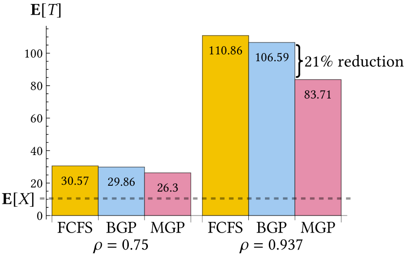
Figure 6.1. Impact of Known Stage Order

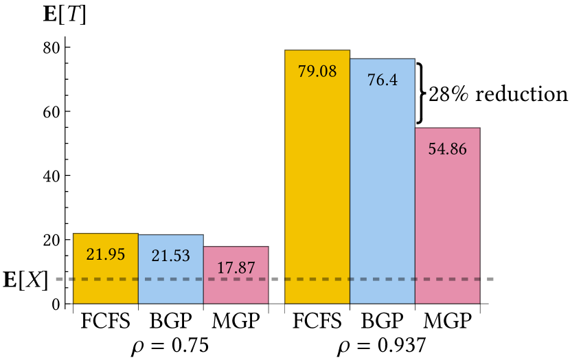
Figure 6.2. Impact of Early Size Information

The first system demonstrates the benefit of knowing the order of a job’s stages. We assume jobs are a mixture of types A , B , and C from Figure 1.2, each with equal probability. Each job has two stages of deterministic size $d=2$ and one stage of stochastic size $S$, which is chosen uniformly from $\{1,12\}$. The different job types correspond to different orderings of these three stages.

• BGP sees every job as having size distribution $S+2d$.

• MGP differentiates jobs based on stage order, which guides its scheduling decisions as shown in Section 6.1.

Figure 6.2 shows MGP reduces mean response time compared to BGP by 12% at moderate load and 21% at high load.

The second system demonstrates the benefit of learning information about a job’s size early. The jobs have type  R from Figure 1.1: they have a diagnosis stage of size $D=1$ followed by either an easy repair stage of size $R_{\text{easy}}=4$ or hard repair stage of size $R_{\text{hard}}=12$. Repair is easy with probability $p=2/3$.

• BGP does not directly learn whether a job is easy or hard to repair, though it can infer it is hard once a job reaches age $5$, at which point it gives the job lower priority than jobs which have not been run yet.

• MGP learns whether a job has easy or hard repair immediately after diagnosis, allowing it to give jobs with hard repairs lower priority sooner.

Figure 6.2 shows MGP reduces mean response time compared to BGP by 17% at moderate load and 28% at high load.

7. Conclusion

In this paper, we introduce multistage jobs, a tool for modeling scheduling problems in which the scheduler has partial but incomplete information about each job’s remaining size. The multistage job model is more general than the standard M/G/1 model with unknown job sizes. The optimal scheduling algorithm for the standard M/G/1, namely the Gittins policy, is complex but tractable. Using a new formulation of the Gittins index called single-job profit (SJP), we are able to reduce the task of optimally scheduling multistage jobs to the task of solving SJP for the job’s individual stages. Finally, we leverage SJP to provide a closed-form analysis of the Gittins policy for multistage jobs, which we use to demonstrate the importance of exploiting multistage structure.

Appendix A Formal Definitions of Job Type Operations

We write $\sqcup$ for disjoint union and let $\mathcal{I}_{\texttt{\scalebox{1.04}{J}}}^{\prime}=\mathcal{I}_{\texttt{\scalebox{1.04}{J}}}\setminus\{z\}$.

Definition A.1.

The state-conditioned job type for job type  J and state $\langle i,x\rangle$, denoted $\texttt{\scalebox{1.04}{J}}\langle i,x\rangle$, is the job type obtained by starting a type  J job in state $\langle i,x\rangle$. Formally, letting $i^{\prime}$ be a new stage label, we define

$$\mathcal{I}_{\texttt{\scalebox{1.04}{J}}\langle i,x\rangle} =(\mathcal{I}_{\texttt{\scalebox{1.04}{J}}}\setminus\{i\})\sqcup\{i^{\prime}\}$$

$$a_{\texttt{\scalebox{1.04}{J}}\langle i,x\rangle} =i^{\prime}$$

$$z_{\texttt{\scalebox{1.04}{J}}\langle i,x\rangle} =z_{\texttt{\scalebox{1.04}{J}}}$$

$$p^{\texttt{\scalebox{1.04}{J}}\langle i,x\rangle}_{jk} =\begin{dcases}p^{\texttt{\scalebox{1.04}{J}}}_{ik}&\text{if }j=i^{\prime}\\ p^{\texttt{\scalebox{1.04}{J}}}_{jk}&\text{otherwise}\\ \end{dcases}$$

$$\mkern 2.4mu\overline{\mkern-2.4muF\mkern-0.8mu}\mkern 0.8mu_{i^{\prime}}(t) =\frac{\mkern 2.4mu\overline{\mkern-2.4muF\mkern-0.8mu}\mkern 0.8mu_{i}(x+t)}{\mkern 2.4mu\overline{\mkern-2.4muF\mkern-0.8mu}\mkern 0.8mu_{i}(x)}.$$

Definition A.2.

The sequential composition of job types J and  K , denoted $\texttt{\scalebox{1.04}{J}}\circ\texttt{\scalebox{1.04}{K}}$, is the job type obtained by “stitching together” J and K . Formally, we define

$$\mathcal{I}_{\texttt{\scalebox{1.04}{J}}\rhd\texttt{\scalebox{1.04}{K}}} =\mathcal{I}_{\texttt{\scalebox{1.04}{J}}}^{\prime}\sqcup\mathcal{I}_{\texttt{\scalebox{1.04}{K}}}$$

$$a_{\texttt{\scalebox{1.04}{J}}\rhd\texttt{\scalebox{1.04}{K}}} =a_{\texttt{\scalebox{1.04}{J}}}$$

$$z_{\texttt{\scalebox{1.04}{J}}\rhd\texttt{\scalebox{1.04}{K}}} =z_{\texttt{\scalebox{1.04}{K}}}$$

$$p^{\texttt{\scalebox{1.04}{J}}\rhd\texttt{\scalebox{1.04}{K}}}_{ij} =\begin{dcases}p^{\texttt{\scalebox{1.04}{J}}}_{ij}&\text{if }i,j\in\mathcal{I}_{\texttt{\scalebox{1.04}{J}}}^{\prime}\\ p^{\texttt{\scalebox{1.04}{J}}}_{iz_{\texttt{\scalebox{1.04}{J}}}}&\text{if }i\in\mathcal{I}_{\texttt{\scalebox{1.04}{J}}}^{\prime}\text{ and }j=a_{\texttt{\scalebox{1.04}{K}}}\\ p^{\texttt{\scalebox{1.04}{K}}}_{ij}&\text{if }i,j\in\mathcal{I}_{\texttt{\scalebox{1.04}{K}}}\\ 0&\text{otherwise.}\end{dcases}$$

Definition A.3.

The single-stage job type with stage $i$, denoted $[i]$, is the job type with just one stage $i$ of size $X_{i}$. Formally, we define $\mathcal{I}_{[i]}=\{a_{[i]}\}=\{i\}$ and $p^{[i]}_{iz}=1$.

Definition A.4.

Let $\mathcal{L}$ be a finite set. The mixture composition of job types $\{\texttt{\scalebox{1.04}{J}}_{\ell}\}_{\ell\in\mathcal{L}}$ with probabilities $\{q_{\ell}\}_{\ell\in\mathcal{L}}$ is the job type representing a job with a randomly chosen type, choosing $\texttt{\scalebox{1.04}{J}}_{\ell}$ with probability $q_{\ell}$. We denote the mixture composition by $\{\texttt{\scalebox{1.04}{J}}_{\ell}\text{ w.p. }q_{\ell}\}_{\ell\in\mathcal{L}}$, abbreviating to $\texttt{\scalebox{1.04}{J}}_{\mathcal{L}}$ when the probabilities are unambiguous. Formally, letting $a^{\prime}$ and $z$ be new stage labels, we define

$$\mathcal{I}_{\texttt{\scalebox{1.04}{J}}_{\mathcal{L}}} =\{a^{\prime},z^{\prime}\}\sqcup\bigsqcup_{\mathclap{\ell\in\mathcal{L}}}\mathcal{I}_{\texttt{\scalebox{1.04}{J}}_{\ell}}^{\prime}$$

$$a_{\texttt{\scalebox{1.04}{J}}_{\mathcal{L}}} =a^{\prime}$$

$$z_{\texttt{\scalebox{1.04}{J}}_{\mathcal{L}}} =z^{\prime}$$

$$p^{\texttt{\scalebox{1.04}{J}}_{\mathcal{L}}}_{ij} =\begin{dcases}q_{\ell}&\text{if }i=a^{\prime}\text{ and }j=a_{\texttt{\scalebox{1.04}{J}}_{\ell}}\\ p^{\texttt{\scalebox{1.04}{J}}_{\ell}}_{iz_{\texttt{\scalebox{1.04}{J}}_{\ell}}}&\text{if }i\in\mathcal{I}_{\texttt{\scalebox{1.04}{J}}_{\ell}}^{\prime}\text{ for some }\ell\in\mathcal{L}\text{ and }j=z^{\prime}\\ p^{\texttt{\scalebox{1.04}{J}}_{\ell}}_{ij}&\text{if }i,j\in\mathcal{I}_{\texttt{\scalebox{1.04}{J}}_{\ell}}^{\prime}\text{ for some }\ell\in\mathcal{L}\\ 0&\text{otherwise}\end{dcases}$$

$$X_{a^{\prime}} =0.$$

Appendix B Algorithm Details for Discrete Stage Size Distributions

To finish the algorithm given in Section 4.2, it remains to

• compute $V_{[i]}$ in $O(|X_{i}|)$ time and

• compose $V_{\texttt{\scalebox{1.04}{K}}}\circ V_{[i]}\circ V_{\texttt{\scalebox{1.04}{L}}}$ in $O(|\texttt{\scalebox{1.04}{K}}|+|X_{i}|+|\texttt{\scalebox{1.04}{L}}|)$ time.

Both of these are made possible by representing the SJP functions by linked lists. This is possible because a job with finite state space has finitely many stopping policies $\pi$, so by Definition 3.1, the SJP function of a job with finite state space is the maximum of finitely many linear functions. Specifically, given

$$0=s_{0}\leq s_{1} \leq\dots\mkern 0.0mu\leq s_{n}$$

$$0=\sigma_{0}\leq\sigma_{1} \leq\dots\mkern 0.0mu\leq\sigma_{n}=1,$$

the list $((s_{1},\sigma_{1}),\dots\mkern 0.0mu,(s_{n},\sigma_{n}))$ represents the following function, which has $V(0)=0$ and slope $\sigma_{k}$ over the interval $(s_{k},s_{k+1})$:

$$V(r)=\begin{dcases}0&r<s_{1}\\ \dots\mkern 0.0mu\\ \sigma_{k}(r-s_{k})+\sum_{\ell=1}^{\mathclap{k-1}}\sigma_{\ell}(s_{\ell+1}-s_{\ell})&s_{k}\leq r<s_{k+1}\\ \dots\mkern 0.0mu\\ r-s_{n}+\sum_{\ell=1}^{\mathclap{n-1}}\sigma_{\ell}(s_{\ell+1}-s_{\ell})&r>s_{n}.\end{dcases}$$

With this representation, we can compute the composition of two functions by traversing the two lists. Each node of one of the input lists transforms to become a node of the output list, with the ordering given by interleaving the input lists. Both the transformation and interleaving can be determined in a manner similar to the “merge” step of merge sort: we examine the first items of both lists, choose one of them to transform, add the transformed item to the output list, remove the original item from its input list, and repeat. This interleaving takes linear time, as desired.

It remains only to compute a single-stage profit function in linear time. Consider the single-stage job $[i]$ with size distribution

$$X_{i}=\begin{dcases}x_{1}&\text{with probability }p_{1}\\ \dots\mkern 0.0mu\\ x_{n}&\text{with probability }p_{n}.\end{dcases}$$

It is convenient to set $x_{0}=0$ and $p_{0}=0$, and we assume for ease of exposition that $x_{1}>0$. We begin by precomputing

$$P_{k} =\mathbf{P}\{X_{i}>x_{k}\}=1-\sum_{\ell=0}^{\mathclap{k-1}}p_{\ell}$$

$$E_{k} =\mathbf{E}[\min\{X_{i},x_{k}\}]=\sum_{\ell=0}^{\mathclap{k-1}}P_{\ell}(x_{\ell+1}-x_{\ell})$$

for $0\leq k\leq n$, which takes $O(n)$ time. To clarify, $P_{0}=0$ and $E_{0}=0$. For brevity, we write $M_{k}=M_{[i]\langle i,x_{\ell}\rangle}$. In this finite-support case, Definition 3.4 and Proposition 3.6 imply

$$M_{k}=\min_{\mathclap{m>k}}\frac{E_{m}-E_{k}}{P_{m}-P_{k}}.$$

We denote the minimizing $m$ by $m(k)$. For any $k<\ell$, it is straightforward to show that the following conditions are equivalent:

• $M_{k}\leq M_{\ell}$,

• $m(k)\leq\ell$, and

• $(E_{\ell}-E_{k})/(P_{\ell}-P_{k})\leq M_{\ell}$.

The third inequality means that if we know $M_{\ell}$, we can obtain the results of the first two comparisons in $O(1)$ time.

Imagine that $1,\dots\mkern 0.0mu,n$ are people standing in a line looking to the right, and suppose that person $k$ has height $M_{k}$. We say that person $k$ sees person $\ell>k$ if $M_{m}\leq M_{k}\leq M_{\ell}$ for all $k<m<\ell$. That is, $k$ sees $\ell$ if $\ell$ is taller than $k$ and there is nobody even taller in the way.

Starting with the base case $M_{n-1}=x_{n}-x_{n-1}$, we now compute $M_{k}$ for $k=n-1,\dots\mkern 0.0mu,0$. We maintain a stack such that after we have computed $M_{k+1}$, the stack contains each person $\ell$ that $k+1$ can see in ascending order. To compute $M_{k}$, we pop people off the stack until $k$ can see the first person $\ell$ on the stack, at which point we push $k$ onto the stack. We have defined seeing such that $m(k)=\ell$, from which we obtain $M_{k}$. It is simple to see that we maintain the invariant. Each person can only be pushed onto and popped off of the stack once, so this entire process takes $O(n)$ time. Given $M_{0},\dots\mkern 0.0mu,M_{n-1}$, we can obtain $V_{0}($) in $O(n)$ time using the approach described at the end of Section 4.1.

Appendix C Deferred Proofs

Proof of Lemma 5.7.

Taking as given that

$$\Phi_{\text{B}}[r](\vec{\imath x})=\Phi_{\text{C}}[s[r]](\vec{\imath x})=\frac{\Phi_{\text{A}}[r](\vec{\imath x})}{1-\rho[r]},$$

we show

• $\Phi_{\text{B}}[r]$ satisfies the optimality equation (5.5/B*) and

• $\Phi_{\text{C}}[s[r]]$ satisfies the optimality equation (5.6/C*), using $s[r]$ as the expected bypass time.

We start by verifying (5.5/B*). Using Lemma 5.3, we compute

(C.1) $$\Lambda\Phi_{\text{B}}[r](\dots\mkern 0.0mu) =\frac{\Lambda\Phi_{\text{A}}[r](\dots\mkern 0.0mu)}{1-\rho[r]}$$

(C.2) $$=\frac{\lambda(\Phi_{\text{A}}[r](\dots\mkern 0.0mu,\langle a,0\rangle)-\Phi_{\text{A}}[r](\dots\mkern 0.0mu))}{1-\rho[r]}$$

(C.3) $$=\frac{\rho[r]}{1-\rho[r]}.$$

Because $\Phi_{\text{A}}[r]$ satisfies (5.4/A*), by pulling out the common $\Lambda\Phi_{\text{B}}[r](\vec{\imath x})$ terms below, we obtain

$$\min_{k}\min\biggl{\{}\begin{matrix}(\Delta_{k}+\Lambda)\Phi_{\text{B}}[r](\vec{\imath x})\\ (\Gamma_{k}[r]+\Lambda)\Phi_{\text{B}}[r](\vec{\imath x})\end{matrix}\biggr{\}} =\min_{k}\min\biggl{\{}\begin{matrix}\Delta_{k}\Phi_{\text{B}}[r](\vec{\imath x})\\ \Gamma_{k}[r]\Phi_{\text{B}}[r](\vec{\imath x})\end{matrix}\biggr{\}}+\frac{\rho[r]}{1-\rho[r]}$$

$$=\frac{1}{1-\rho[r]}\min_{k}\min\biggl{\{}\begin{matrix}\Delta_{k}\Phi_{\text{A}}[r](\vec{\imath x})\\ \Gamma_{k}[r]\Phi_{\text{A}}[r](\vec{\imath x})\end{matrix}\biggr{\}}+\frac{\rho[r]}{1-\rho[r]}$$

$$=-1,$$

which, as desired, is (5.5/B*).

We now turn to verifying (5.6/C*). Because $\Phi_{\text{B}}[r](\vec{\imath x})$ satisfies (5.5/B*), we know $\Phi_{\text{C}}[s[r]](\vec{\imath x})$ satisfies the “top branch” of (5.6/C*). It thus suffices to show the “bottom branch”

$$\Gamma_{k}[s[r]]\Phi_{\text{B}}[s[r]](\vec{\imath x})\geq-1,$$

with equality if $(\Gamma_{k}[r]+\Lambda)\Phi_{\text{B}}[s[r]](\vec{\imath x})=-1$. Recalling (C.1), we compute

$$\Gamma_{k}[s[r]]\Phi_{\text{B}}[r](\vec{\imath x}) =\Gamma_{k}\biggl{[}\frac{r}{1-\rho[r]}\biggr{]}\Phi_{\text{B}}[r](\vec{\imath x})$$

$$=\frac{1-\rho[r]}{r}(\Phi_{\text{B}}[r](\dots\mkern 0.0mu,\langle z,0\rangle,\dots\mkern 0.0mu)-\Phi_{\text{B}}[r](\dots\mkern 0.0mu,\langle i_{k},x_{k}\rangle,\dots\mkern 0.0mu))$$

$$=(1-\rho[r])\Gamma_{k}[r]\Phi_{\text{B}}[r](\vec{\imath x})$$

$$=(1-\rho[r])(\Gamma_{k}[r]+\Lambda)\Phi_{\text{B}}[r](\vec{\imath x})-\rho[r].$$

$$\geq-1,$$

with equality if $(\Gamma_{k}[r]+\Lambda)\Phi_{\text{B}}[r](\vec{\imath x})=-1$, as desired. ∎

Proof of Lemma 5.10.

We follow much the same argument as for Lemma 3.2. It is clear that $\Phi_{\text{C}}[0](\langle i,x\rangle)=0$, so it suffices to show that $\Phi_{\text{C}}[s](\langle i,x\rangle)$ is

1. concave and nondecreasing in $s$, which implies decreasing derivative bounded below by $0$; and

2. bounded above by $s$, which implies derivative bounded above by $1$.

Given a fixed policy for BPOP C, the expected cost is

$$s\mathbf{E}[\text{number of bypassed jobs}]+\mathbf{E}[\text{time spent on all jobs}],$$

which is concave and nonincreasing in $s$. The cost $\Phi_{\text{C}}[s](\langle i,x\rangle)$ is the infimum of all such functions, implying claim i. A possible policy is to bypass the job immediately, which has expected cost $s$, implying claim ii. ∎

Proof of Lemma 5.11.

By Lemma 5.7, if $r\leq M_{\langle i,x\rangle}$,

$$\Phi_{\text{C}}[s[r]](\langle i,x\rangle) =\frac{\Phi_{\text{A}}[r](\langle i,x\rangle)}{1-\rho[r]}$$

$$=\frac{r}{1-\rho[r]}$$

$$=s[r].$$

This means that for all $s<s[M_{\langle i,x\rangle}]$,

$$\mathbf{P}\{S_{\langle i,x\rangle}>s\}=\frac{d}{ds}\Phi_{\text{C}}[s](\langle i,x\rangle)=1,$$

so $\mathbf{P}\{S_{\langle i,x\rangle}\geq s[M_{\langle i,x\rangle}]\}=1$. ∎

Proof of Lemma 5.12.

By the same reasoning as (5.9),

$$\varphi_{k\ell}(\vec{\imath x})=\mathbf{E}[\Phi_{\text{C}}[S_{\langle i_{\ell},x_{\ell}\rangle}](\langle i_{k},x_{k}\rangle)].$$

Because $\Phi_{\text{C}}[s](\vec{\imath x})$ satisfies (5.6/C*),

(C.4) $$(\Delta_{k}+\Lambda)\varphi_{k\ell}(\vec{\imath x})=\mathbf{E}[(\Delta_{k}+\Lambda)\Phi_{\text{C}}[S_{\langle i_{\ell},x_{\ell}\rangle}](\langle i_{k},x_{k}\rangle)]\geq-1,$$

where we continue to slightly abuse the $\Delta_{k}$ notation. The same argument holds with $k$ and $\ell$ swapped. It remains only to show that (C.4) is actually an equality, which requires the $M_{\langle i_{k},x_{k}\rangle}\leq M_{\langle i_{\ell},x_{\ell}\rangle}$ hypothesis. By Lemma 5.11, we have $\mathbf{P}\{s[M_{\langle i_{k},x_{k}\rangle}]\leq S_{\langle i_{\ell},x_{\ell}\rangle}\}=1$. Thus, to prove (C.4) is an equality, it suffices to show that for any $r\geq M_{\langle i_{k},x_{k}\rangle}$,

$$(\Delta_{k}+\Lambda)\Phi_{\text{C}}[s[r]](\langle i_{k},x_{k}\rangle)=-1,$$

because $s[r]$ for $r\geq M_{\langle i_{k},x_{k}\rangle}$ covers all possible values of $S_{\langle i_{\ell},x_{\ell}\rangle}$. Using (C.1) and Lemma 5.7, we compute

$$(\Delta_{k}+\Lambda)\Phi_{\text{C}}[s[r]](\langle i_{k},x_{k}\rangle) =(\Delta_{k}+\Lambda)\Phi_{\text{B}}[r](\langle i_{k},x_{k}\rangle)$$

$$=\Delta_{k}\Phi_{\text{B}}[r](\langle i_{k},x_{k}\rangle)+\frac{\rho[r]}{1-\rho[r]}$$

$$=\frac{1}{1-\rho[r]}\Delta_{k}\Phi_{\text{A}}[r](\langle i_{k},x_{k}\rangle)+\frac{\rho[r]}{1-\rho[r]}.$$

Because $r\geq M_{\langle i_{k},x_{k}\rangle}$, it is optimal to serve job $k$ in BPOP A with expected bypass time $r$. This means $\Delta_{k}\Phi_{\text{A}}[r](\langle i_{k},x_{k}\rangle)=-1$, which completes the computation as desired. ∎

Proof of Lemma 5.13.

For all stages $j\neq i$, the probability $q_{ij}$ satisfies $q_{ij}=\sum_{k\in\mathcal{I}}p_{ik}q_{kj}$, which means

(C.5) $$\sum_{j\neq i}p_{ij}\varphi(\langle j,0\rangle)-\varphi(\langle i,x\rangle)=-\mkern-3.5mu\int\displaylimits_{x}^{\infty}\mkern-3.5mu\frac{\mkern 2.4mu\overline{\mkern-2.4muF\mkern-0.8mu}\mkern 0.8mu_{i}(y)}{\mkern 2.4mu\overline{\mkern-2.4muF\mkern-0.8mu}\mkern 0.8mu_{i}(x)}\alpha(\langle i,y\rangle)\,dy.$$

The second term of $\varphi(\langle i,x\rangle)$ is constant in $x$, so using the Leibniz integral rule, we compute

$$\frac{d}{dx}\varphi(\langle i,x\rangle) =\frac{d}{dx}\mkern-3.5mu\int\displaylimits_{x}^{\infty}\mkern-3.5mu\frac{\mkern 2.4mu\overline{\mkern-2.4muF\mkern-0.8mu}\mkern 0.8mu_{i}(y)}{\mkern 2.4mu\overline{\mkern-2.4muF\mkern-0.8mu}\mkern 0.8mu_{i}(x)}\alpha(\langle i,y\rangle)\,dy$$

$$=\frac{f_{i}(x)}{(\mkern 2.4mu\overline{\mkern-2.4muF\mkern-0.8mu}\mkern 0.8mu_{i}(x))^{2}}\mkern-3.5mu\int\displaylimits_{x}^{\infty}\mkern-3.5mu\mkern 2.4mu\overline{\mkern-2.4muF\mkern-0.8mu}\mkern 0.8mu_{i}(y)\alpha(\langle i,y\rangle)\,dy+\frac{1}{\mkern 2.4mu\overline{\mkern-2.4muF\mkern-0.8mu}\mkern 0.8mu_{i}(x)}\mkern-2.5mu\cdot\mkern-2.5mu\frac{d}{dx}\mkern-3.5mu\int\displaylimits_{x}^{\infty}\mkern-3.5mu\mkern 2.4mu\overline{\mkern-2.4muF\mkern-0.8mu}\mkern 0.8mu_{i}(y)\alpha(\langle i,y\rangle)\,dy$$

$$=h_{i}(x)\mkern-3.5mu\int\displaylimits_{x}^{\infty}\mkern-3.5mu\frac{\mkern 2.4mu\overline{\mkern-2.4muF\mkern-0.8mu}\mkern 0.8mu_{i}(y)}{\mkern 2.4mu\overline{\mkern-2.4muF\mkern-0.8mu}\mkern 0.8mu_{i}(x)}\alpha(\langle i,y\rangle)\,dy-\alpha(\langle i,x\rangle),$$

which with (C.5) yields $\Delta_{1}\varphi(\langle i,x\rangle)=-\alpha(\langle i,x\rangle)$, as desired. ∎

Proof of Proposition 6.1.

Clearly $V_{[i]}(r)=\max\{0,r-d\}$ and $M_{[i]}=d$, so by Definition 3.3 and Theorem 4.2,

$$M_{\texttt{\scalebox{1.04}{J}}\rhd[i]} =V^{-1}_{\texttt{\scalebox{1.04}{J}}}(d)$$

$$M_{[i]\rhd\texttt{\scalebox{1.04}{J}}} =M_{\texttt{\scalebox{1.04}{J}}}+d.$$

Lemma 3.2 implies

$$V_{\texttt{\scalebox{1.04}{J}}}(M_{[i]\rhd\texttt{\scalebox{1.04}{J}}})\leq d=V_{\texttt{\scalebox{1.04}{J}}}(M_{\texttt{\scalebox{1.04}{J}}\rhd[i]}).$$

Again by Lemma 3.2, $V_{\texttt{\scalebox{1.04}{J}}}(r)$ is strictly increasing for $r\geq M_{\texttt{\scalebox{1.04}{J}}}$, which means $M_{[i]\rhd\texttt{\scalebox{1.04}{J}}}\leq M_{\texttt{\scalebox{1.04}{J}}\rhd[i]}$. ∎

Appendix D Spurious Solutions to Optimality Equations

Before addressing the specific optimality equations in Section 5.2, we give a simple example which illustrates the main source of spurious solutions and our method for ruling them out.

D.1. Warmup: Computing Expectation with Dynamic Programming

Consider a single-stage job with continuous size distribution $X$, which has density, tail, and hazard rate functions $f$, $\mkern 2.4mu\overline{\mkern-2.4muF\mkern-0.8mu}\mkern 0.8mu$, and $h$, respectively. As usual, we assume $\mathbf{E}[X]$ is finite. For ease of exposition, we assume $X$ has unbounded support, but the arguments can be easily modified to handle the bounded case.

Let $\varphi(x)=\mathbf{E}[X-x\nonscript\>|\nonscript\>\mathopen{}X>x]$ be the job’s expected remaining size at age $x$. We can think of $\varphi$ as the cost function of the dynamic program with a single action, namely serving the job, that incurs cost at continuous rate $1$ until the job completes. The optimality equation for this dynamic program is, by analogy with Definition 5.2,

(D.1) $$\frac{d}{dx}\varphi(x)+h(x)(\varphi({})-\varphi(x))=-1,$$

where $\varphi({})=0$. Solving this equation yields a family of solutions parametrized by $c\in\mathds{R}$:

$$\varphi_{c}(x)=\frac{c}{\mkern 2.4mu\overline{\mkern-2.4muF\mkern-0.8mu}\mkern 0.8mu(x)}+\mkern-3.5mu\int\displaylimits_{x}^{\infty}\mkern-3.5mu\frac{\mkern 2.4mu\overline{\mkern-2.4muF\mkern-0.8mu}\mkern 0.8mu(y)}{\mkern 2.4mu\overline{\mkern-2.4muF\mkern-0.8mu}\mkern 0.8mu(x)}\,dy.$$

The true cost function is $\varphi_{0}$, so we need a criterion that rules out solutions with $c\neq 0$. In this case, a sufficient condition is

(D.2) $$\lim_{\mathclap{x\to\infty}}\mkern 2.4mu\overline{\mkern-2.4muF\mkern-0.8mu}\mkern 0.8mu(x)|\varphi(x)|=0.$$

To see why (D.2) suffices, observe that because $\mathbf{E}[X]$ is finite,

$$\lim_{\mathclap{x\to\infty}}\mkern 2.4mu\overline{\mkern-2.4muF\mkern-0.8mu}\mkern 0.8mu(x)|\varphi_{0}(x)|=\lim_{\mathclap{x\to\infty}}\ \ \mkern-3.5mu\int\displaylimits_{x}^{\infty}\mkern-3.5mu\mkern 2.4mu\overline{\mkern-2.4muF\mkern-0.8mu}\mkern 0.8mu(y)\,dy=0,$$

so $\lim_{x\to\infty}\mkern 2.4mu\overline{\mkern-2.4muF\mkern-0.8mu}\mkern 0.8mu(x)|\varphi_{c}(x)|=|c|$. Therefore, to show that $\varphi_{0}$ is the true cost function, it suffices to show that the true cost function must satisfy (D.2), which we write more succinctly as $\varphi(x)=o(1/\mkern 2.4mu\overline{\mkern-2.4muF\mkern-0.8mu}\mkern 0.8mu(x))$.

For the trivial dynamic program in this example, the simplest way to show $\varphi(x)=o(1/\mkern 2.4mu\overline{\mkern-2.4muF\mkern-0.8mu}\mkern 0.8mu(x))$ is to compute the expected remaining size directly, which removes the need to solve the optimality equation at all. However, as we will soon see, we can give asymptotic bounds similar to $o(1/\mkern 2.4mu\overline{\mkern-2.4muF\mkern-0.8mu}\mkern 0.8mu(x))$ for BPOP Q, even though directly computing its cost function $\Phi_{\text{Q}}$ is intractable.

D.2. Ruling Out Spurious Solutions for BPOP Q

There are two steps to ruling out spurious solutions to (5.3/Q*). We first show that $\Phi_{\text{Q}}$ has a “quadratic” form, meaning

(D.3) $$\Phi_{\text{Q}}(\vec{\imath x})=\sum_{k}\varphi_{1}(\langle i_{k},x_{k}\rangle)+\sum_{\mathclap{k<\ell}}\varphi_{2}(\langle i_{k},x_{k}\rangle,\langle i_{\ell},x_{\ell}\rangle)$$

for some functions $\varphi_{1}$ and $\varphi_{2}$. We compute $\varphi_{1}$ in terms of $\varphi_{2}$ and asymptotically bound $\varphi_{2}$ similarly to (D.2), which rules out all spurious solutions to (5.3/Q*).

We begin by establishing that $\Phi_{\text{Q}}$ has the quadratic form given by (D.3). We recursively define the busy period started by job $k\kern-0.5pt$, denoted $\mathcal{B}_{k}$, to be the smallest set of jobs containing

• job $k$ itself and

• all jobs that arrive while serving any job in the busy period started by job $k$.

Given any system state, let $\varphi_{2}(\langle i_{k},x_{k}\rangle,\langle i_{\ell},x_{\ell}\rangle)$ be the total expected queueing time in the remainder of the busy period due to jobs in $\mathcal{B}_{k}$ waiting while jobs in $\mathcal{B}_{\ell}$ are in service, plus vice versa. We call this the “interference” between $\mathcal{B}_{k}$ and $\mathcal{B}_{\ell}$. To clarify, when there are $n$ jobs from $\mathcal{B}_{k}$ in the system, then each instant serving a job in $\mathcal{B}_{\ell}$ counts for $n$ instants of queueing time.

The key observation is that interference is well defined, even though it does not account for all jobs in the system. This is because for the purposes of determining the interference between $\mathcal{B}_{k}$ and $\mathcal{B}_{\ell}$ we can imagine a separate “$\mathcal{B}_{k}$ vs. $\mathcal{B}_{\ell}$” process which is paused whenever a job not in $\mathcal{B}_{k}$ or $\mathcal{B}_{\ell}$ is in service. Because the arrival process is Poisson and the Gittins policy is an index policy, the $\mathcal{B}_{k}$ vs. $\mathcal{B}_{\ell}$ process is unaffected by other jobs in the system.

The second term on the right-hand side of (D.3) accounts for all the remaining expected queueing time from state $\vec{\imath x}$ except for that incurred “within” each $\mathcal{B}_{k}$. We therefore define $\varphi_{1}(\langle i_{k},x_{k}\rangle)$ to be the total expected queueing time due to jobs in $\mathcal{B}_{k}$ waiting while other jobs in $\mathcal{B}_{k}$ are in service, which we can show is well defined by an argument similar to that for $\varphi_{2}$ above. This establishes that $\Phi_{\text{Q}}$ has the quadratic from of (D.3).

We now compute $\varphi_{1}$ in terms of $\varphi_{2}$. If a new job $k^{\prime}$ arrives when job $k$ is in state $\langle j,y\rangle$, then the interference between $\mathcal{B}_{k}$ and $\mathcal{B}_{k^{\prime}}$ from that point onward is $\varphi_{2}(\langle j,y\rangle,\langle a,0\rangle)$. From this observation we directly compute

$$\varphi_{1}(\langle i,x\rangle) =\mkern-3.5mu\int\displaylimits_{x}^{\infty}\mkern-3.5mu\lambda\frac{\mkern 2.4mu\overline{\mkern-2.4muF\mkern-0.8mu}\mkern 0.8mu_{i}(y)}{\mkern 2.4mu\overline{\mkern-2.4muF\mkern-0.8mu}\mkern 0.8mu_{i}(x)}\varphi_{2}(\langle i,y\rangle,\langle a,0\rangle)\,dy$$

$$\qquad+\sum_{\mathclap{j\neq i}}\mkern 3.0mu\mkern-3.5mu\int\displaylimits_{0}^{\infty}\mkern-3.5mu\lambda q_{ij}\mkern 2.4mu\overline{\mkern-2.4muF\mkern-0.8mu}\mkern 0.8mu_{j}(y)\varphi_{2}(\langle j,y\rangle,\langle a,0\rangle)\,dy,$$

where $q_{ij}$ is the probability that a job starting in stage $i$ at some point reaches stage $j$.

It remains only to characterize $\varphi_{2}$. It is immediate from applying (D.3) to a system state with one job that $\varphi_{1}(\langle i,x\rangle)=\Phi_{\text{Q}}(\langle i,x\rangle)$. By applying (5.3/Q*) to a system state with two jobs, we obtain

(D.4) $$\min_{k}(\Delta_{k}+\Lambda)\varphi_{2}(\langle i_{1},x_{1}\rangle,\langle i_{2},x_{2}\rangle)=-1$$

Our next step is to turn this into a single-variable differential equation similar to (D.1). To do so, we consider the evolution of the system assuming that no arrivals or state transitions occur. We define $x_{1}(t)$, $x_{2}(t)$ and $k(t)$ such that

$$x_{1}(t)-x_{1} =t-(x_{2}(t)-x_{2})=\mkern-3.5mu\int\displaylimits_{0}^{t}\mkern-3.5mu(2-k(t))\,dt$$

$$k(t) =\operatorname*{arg\,min}_{k}\Delta_{k}\varphi_{2}(\langle i_{1},x_{1}\rangle,\langle i_{2},x_{2}\rangle).$$

That is, starting from system state $(\langle i_{1},x_{1}\rangle,\langle i_{2},x_{2}\rangle)$ and assuming no arrivals or stage transitions, $x_{1}(t)$ and $x_{2}(t)$ are the ages of the stages at time $t$ and $k(t)$ is the job being served at time $t$.

Suppose temporarily that stages $i_{1}$ and $i_{2}$ are penultimate stages, meaning they transition only to the final stage $z$. By (D.4),

(D.5) $$\frac{d}{dt}\varphi_{2}(t)-h_{k(t)}(x_{k(t)})\varphi_{2}(t)=-(1+\Lambda\varphi_{2}(t)),$$

where we abbreviate $\varphi_{2}(t)=\varphi_{2}(\langle i_{1},x_{1}(t)\rangle,\langle i_{2},x_{2}(t)\rangle)$. We can interpret $h_{Y}(t)=h_{k(t)}(x_{k(t)})$ as the hazard rate of a random variable $Y$, which is the time of the first stage transition. It is straightforward to show that finiteness of $\mathbf{E}[X_{1}]$ and $\mathbf{E}[X_{2}]$ implies finiteness of $\mathbf{E}[Y]$. We can use $Y$ to express the possible solutions for $\varphi_{2}(t)$:

(D.6) $$\varphi_{2}(t)=\frac{c}{\mkern 2.4mu\overline{\mkern-2.4muF\mkern-0.8mu}\mkern 0.8mu_{Y}(t)}+\mkern-3.5mu\int\displaylimits_{t}^{\infty}\mkern-3.5mu\lambda\frac{\mkern 2.4mu\overline{\mkern-2.4muF\mkern-0.8mu}\mkern 0.8mu_{Y}(u)}{\mkern 2.4mu\overline{\mkern-2.4muF\mkern-0.8mu}\mkern 0.8mu_{Y}(t)}(1+\Lambda\varphi_{2}(t))\,du.$$

Confirming (5.15) entails showing $c=0$. By considering the policy that prioritizes new arrivals above jobs $1$ and $2$, performing the preemptive last-come, first-served (PLCFS) policy [13] on the new arrivals, we obtain the bound

$$\varphi_{2}(t)\leq\frac{\rho\mathbf{E}[Y-t\nonscript\>|\nonscript\>\mathopen{}Y\geq t]}{(1-\rho)^{2}}=o\biggl{(}\frac{1}{\mkern 2.4mu\overline{\mkern-2.4muF\mkern-0.8mu}\mkern 0.8mu_{Y}(t)}\biggr{)},$$

so $c=0$ in (D.6), as desired.

We assumed temporarily that stages $i_{1}$ and $i_{2}$ were penultimate stages. Because there are no cyclic stage transitions, we can iterate the argument to cover every stage. The only change is an extra term on the right-hand side of (D.5), which does not substantially change the argument.

References

- [1]
- Aalto et al. [2009] Samuli Aalto, Urtzi Ayesta, and Rhonda Righter. 2009. On the Gittins index in the M/G/1 queue. Queueing Systems 63, 1 (2009), 437–458.
- Aalto et al. [2011] Samuli Aalto, Urtzi Ayesta, and Rhonda Righter. 2011. Properties of the Gittins index with application to optimal scheduling. Probability in the Engineering and Informational Sciences 25, 03 (2011), 269–288.
- Bertsimas [1995] Dimitris Bertsimas. 1995. The achievable region method in the optimal control of queueing systems; formulations, bounds and policies. Queueing systems 21, 3 (1995), 337–389.
- Bertsimas et al. [1995] Dimitris Bertsimas, Ioannis Ch Paschalidis, and John N Tsitsiklis. 1995. Branching bandits and Klimov’s problem: Achievable region and side constraints. IEEE Trans. Automat. Control 40, 12 (1995), 2063–2075.
- Chakravorty and Mahajan [2014] Jhelum Chakravorty and Aditya Mahajan. 2014. Multi-armed bandits, Gittins index, and its calculation. Methods and applications of statistics in clinical trials: Planning, analysis, and inferential methods 2 (2014), 416–435.
- Davis [1984] Mark H. A. Davis. 1984. Piecewise-deterministic Markov processes: A general class of non-diffusion stochastic models. Journal of the Royal Statistical Society. Series B (Methodological) (1984), 353–388.
- Dumitriu et al. [2003] Ioana Dumitriu, Prasad Tetali, and Peter Winkler. 2003. On playing golf with two balls. SIAM Journal on Discrete Mathematics 16, 4 (2003), 604–615.
- Frostig and Weiss [1999] Esther Frostig and Gideon Weiss. 1999. Four proofs of Gittins’ multiarmed bandit theorem. Annals of Operations Research (1999), 1–39.
- Gittins [1979] John C. Gittins. 1979. Bandit Processes and Dynamic Allocation Indices. Journal of the Royal Statistical Society. Series B (Methodological) 41, 2 (1979), 148–177.
- Gittins et al. [2011] John C. Gittins, Kevin D. Glazebrook, and Richard Weber. 2011. Multi-armed Bandit Allocation Indices. John Wiley & Sons.
- Gittins and Jones [1974] John C. Gittins and David M. Jones. 1974. A Dynamic Allocation Index for the Sequential Design of Experiments. In Progress in Statistics, J. Gani (Ed.). North-Holland, Amsterdam, NL, 241–266.
- Harchol-Balter [2013] Mor Harchol-Balter. 2013. Performance Modeling and Design of Computer Systems: Queueing Theory in Action (1st ed.). Cambridge University Press, New York, NY, USA.
- Hyytiä et al. [2012] Esa Hyytiä, Samuli Aalto, and Aleksi Penttinen. 2012. Minimizing slowdown in heterogeneous size-aware dispatching systems. In ACM SIGMETRICS Performance Evaluation Review, Vol. 40. ACM, 29–40.
- Kleinrock [1976] Leonard Kleinrock. 1976. Queueing Systems, Volume 2: Computer Applications. Vol. 66. Wiley New York.
- Klimov [1975] G. P. Klimov. 1975. Time-Sharing Service Systems. I. Theory of Probability And Its Applications 19, 3 (1975), 532–551.
- Osipova et al. [2009] Natalia Osipova, Urtzi Ayesta, and Konstantin Avrachenkov. 2009. Optimal policy for multi-class scheduling in a single server queue. In Teletraffic Congress, 2009. ITC 21 2009. 21st International. IEEE, 1–8.
- Schrage [1967] Linus E Schrage. 1967. The queue M/G/1 with feedback to lower priority queues. Management Science 13, 7 (1967), 466–474.
- Schrage and Miller [1966] Linus E Schrage and Louis W Miller. 1966. The queue M/G/1 with the shortest remaining processing time discipline. Operations Research 14, 4 (1966), 670–684.
- Scully et al. [2018] Ziv Scully, Mor Harchol-Balter, and Alan Scheller-Wolf. 2018. SOAP: One Clean Analysis of All Age-Based Scheduling Policies. Proc. ACM Meas. Anal. Comput. Syst. 2, 1, Article 16 (April 2018), 30 pages. https://doi.org/10.1145/3179419
- Vermes [1985] D. Vermes. 1985. Optimal control of piecewise deterministic Markov process. Stochastics 14, 3 (1985), 165–207.
- Weber [1992] Richard Weber. 1992. On the Gittins index for multiarmed bandits. The Annals of Applied Probability 2, 4 (1992), 1024–1033.
- Weiss [1995] Gideon Weiss. 1995. On almost optimal priority rules for preemptive scheduling of stochastic jobs on parallel machines. Advances in Applied Probability 27, 3 (1995), 821–839.
- Whittle [1980] Peter Whittle. 1980. Multi-armed bandits and the Gittins index. Journal of the Royal Statistical Society. Series B (Methodological) (1980), 143–149.
- Whittle [2005] Peter Whittle. 2005. Tax problems in the undiscounted case. Journal of applied probability 42, 03 (2005), 754–765.