Learning non-smooth models: instrumental variable quantile regressions and related problems

Abstract

This paper proposes computationally efficient methods that can be used for instrumental variable quantile regressions (IVQR) and related methods with statistical guarantees. This is much needed when we investigate heterogenous treatment effects since interactions between the endogenous treatment and control variables lead to an increased number of endogenous covariates. We prove that the GMM formulation of IVQR is NP-hard and finding an approximate solution is also NP-hard. Hence, solving the problem from a purely computational perspective seems unlikely. Instead, we aim to obtain an estimate that has good statistical properties and is not necessarily the global solution of any optimization problem.

The proposal consists of employing $k$-step correction on an initial estimate. The initial estimate exploits the latest advances in mixed integer linear programming and can be computed within seconds. One theoretical contribution is that such initial estimators and Jacobian of the moment condition used in the $k$-step correction need not be even consistent and merely $k=4\log n$ fast iterations are needed to obtain an efficient estimator. The overall proposal scales well to handle extremely large sample sizes because lack of consistency requirement allows one to use a very small subsample to obtain the initial estimate and the $k$-step iterations on the full sample can be implemented efficiently. Another contribution that is of independent interest is to propose a tuning-free estimation for the Jacobian matrix, whose definition nvolves conditional densities. This Jacobian estimator generalizes bootstrap quantile standard errors and can be efficiently computed via closed-end solutions. We evaluate the performance of the proposal in simulations and an empirical example on the heterogeneous treatment effect of Job Training Partnership Act.

1 Introduction

The linear instrumental variables quantile model (IVQR) formulated by Chernozhukov and Hansen, (2005, 2006, 2008) has found wide applications in economics. The basic moment condition can be written as follows

$$Y_{i}=X_{i}^{\prime}\beta_{*}+\varepsilon_{i}\qquad{\rm and}\qquad P(\varepsilon_{i}\leq 0\mid Z_{i})=\tau,$$ (1)

where $\tau\in(0,1)$ is the quantile of interest, $Y_{i}\in\mathbb{R}$, $X_{i}\in\mathbb{R}^{p}$ and $Z_{i}\in\mathbb{R}^{L}$ are i.i.d observed variables and $\beta_{*}\in\mathbb{R}^{p}$ is the unknown model parameter. Assume that $p$ and $L$ are fixed with $L\geq p$. The typical setup is that only one (or few) component of $X_{i}$ is endogenous and other components of $X_{i}$ are contained in $Z_{i}$. In the policy evaluation setting, the variable denoting the status of treatment is usually considered endogenous. If this variable only enters the regression equation as one endogenous regressor, then we can apply the existing methods (e.g., the popular method by Chernozhukov and Hansen, (2006)) for estimating the treatment effect. When multiple endogenous regressors enter the regression equation, it imposes enormous (or even prohibitive) computational challenges to common estimation strategies, which typically involve solving nonconvex and non-smooth optimization problems.

In empirical studies that investigate the causal effects of an endogenous treatment, multiple endogenous regressors arise naturally. For example, the interactions between the treatment variable and other variables are often included in the regression to study the heterogeneity of the treatment effects. In the IVQR setting, this leads to multiple endogenous variables in the regression equation. Consider the randomized training experiment conducted under the Job Training Partnership Act (JTPA). JTPA training services are randomly offered to people, who can then choose whether to participate in the program. One key policy question is whether this program has an effect on earnings. Of course, the baseline question is whether the program has a positive effect overall. In addition, one might ask questions such as whether the effect of the program differs by participants’ race, age, etc. These questions can be answered in the regression setting by learning the coefficients for interactions between the treatment status and other variables denoting race, age, etc.

We show that the efficient computations for estimating IVQR from a purely algorithmic perspective might not exist. In particular, we prove that optimization of the usual GMM or similar formulation of the IVQR problem is NP (non-deterministic polynomial-time) hard. To the best of our knowledge, this is the first formal statement on the NP-hardness of the IVQR problem. Due to this result, it is unlikely to find a computationally efficient algorithm that minimizes the GMM criterion function. Notice that this is different from some existing methods that cast the GMM problem as NP-hard problems, e.g., mixed integer program or quadratic program with complementarity constraints (Burer and Saxena,, 2012; Chen and Lee,, 2018). These papers only imply that these NP-hard problems are more difficult than IVQR GMM-estimation; in other words, algorithms that solve certain NP-hard problems can be used for IVQR estimation. However, the question of whether there exist simple algorithms for IVQR GMM-estimation is still open. In this paper, we provide a negative answer by showing that IVQR estimation is at least as difficult as the set partition problem, which is known to be NP-hard since Karp, (1972). Moreover, we show that it is also very difficult to find an approximate solution in that obtaining a solution within a constant factor from the global solution is also NP-hard. Therefore, there is inherent complexity that is unlikely to be fully handled by convex relaxation, smoothing or other pure computational remedies for handling non-convex and non-smooth optimization problems.

The NP-hardness suggests that serious efforts are needed to address the computational challenge, but it does not necessarily mean that the model has to be shunned by practitioners. In fact, some of the most popular methods, such as decision trees and $k$-means clustering (Laurent and Rivest,, 1976; Mahajan et al.,, 2012), are NP-hard. One key observation is that NP-hardness is a statement on the difficulty of the worst-case situation, but the data that arise in practice might not be these “bad” situations. Although optimization algorithms derived from a pure computational point of view are not guaranteed to exploit “probabilistic” properties of the data, there are many inspiring precedents in machine learning that exploit statistical properties to overcome computational difficulties. For example, finding a hyperplane to classify binary targets is a common approach. Whereas using the misclassification rate as the loss function leads to an NP-hard optimization problem, one can use a convex loss function (e.g., hinge loss or logistic loss) and still obtain nice statistical properties, see (Bishop,, 2006; Shalev-Shwartz and Ben-David,, 2014).

Here, we propose to apply the same principle to general non-smooth models. Instead of focusing only on clever computational tricks for the usual GMM formulation, we exploit the statistical aspect of the model and provide an alternative estimation and inference strategy that admits fast computation algorithms. Although estimates from any feasible optimization programs might be of questionable quality, our plan is to use a computationally cheap method and turn a dubious estimate into one with nice statistical properties. Of course, this final estimate might not be the global solution of any optimization problem but good statistical properties would often suffice for estimation and inference purposes.

Our proposal is a $k$-step framework that exploits the identification strength of a general (possibly nonsmooth) GMM model. This framework starts with an initial estimate and updates it iteratively, where each iteration involves only matrix multiplications and no optimization at all. We show that when the identification is strong, only few iterations are needed to obtain an estimator that is asymptotically equivalent to the GMM estimator.

One key finding is that the initial estimator does not need to be consistent. This is a new result as far as we know. We show that there is a neighborhood of the true parameter value whose area is determined by the identification strength and any point in this neighborhood can be used as an initial estimate; when the identification is strong in the usual sense for GMM models (i.e., Jacobian of the population moment has well-behaved singular values), this neighborhood is fixed and its area does not shrink to zero with sample size $n\rightarrow\infty$. Allowing for inconsistent initial estimates provides valuable convenience in practice. When the initial estimates are computed via complicated optimization problems, computationally feasible solutions might not be consistent since they are often not global solutions even under strong identification. Moreover, even if initial estimates are easily obtained via efficient algorithms, these algorithms might not be feasible when the sample size becomes extremely large. For large datasets that arise in modern research, even common convex problems often encounter scalability issues, see e.g., (Yang et al.,, 2013; Lin et al.,, 2017). Since the initial estimate does not need to be even consistent, one can simply compute it using a very small fraction of the entire sample. Efficient algorithms are available for $k$-step iterations as they only require matrix multiplications. This leads to a fast procedure for handling massive datasets.

We also provide methods and theory for two important aspects of implementing the $k$-step framework. First, we provide a tuning-free estimate for the Jacobian matrix of the moment condition. This estimate is needed for the $k$-step correction and can be tricky to obtain in practice. The formula defining the Jacobian typically contains the (conditional) density of a variable and one typical estimation method is to use kernel with a bandwidth choice. However, the bandwidth might be quite difficult to choose in practice. We propose to generalize a fast bootstrap scheme for density estimation. The basic idea is as follows. Consider the estimation of the density of a variable at a point. Since the asymptotic variance of the bootstrapped sample quantile of this variable is directly related to the density, bootstrapping sample quantile can be used to obtain a consistent density estimate. We generalize this approach to estimation of Jacobian of general nonsmooth GMM models. Notice that the Jacobian matrix can be estimated entry by entry. In the case of IVQR, this has a closed-end solution with computation burden similar to bootstrapping sample quantiles; in our experiments, with a sample size $n=5000$, computing 2000 bootstrap samples takes 0.5 second. Since the entire procedure can be used for general GMM settings and does not require choices such as bandwidth, we believe it is of independent interest. For example, one can use it as a tuning-free density estimator, which can be used to compute the optimal bandwidth for a second-stage estimation. We establish the consistency for this estimate.

Second, we present a formulation that yields initial estimators for IV quantile models and related problems via mixed integer linear programs (MILP). Although MILP is also an NP-hard problem, it is one of the most well-studied and well-understood hard problems and so much progress has been made in recent years that many believe large-scale problems are now feasible, see e.g., (Bertsimas and Weismantel,, 2005; Bixby and Rothberg,, 2007; Jünger et al.,, 2009; Linderoth and Lodi,, 2010). As pointed out by Bertsimas et al., (2016), the speed of finding global solutions for mixed integer optimization improved approximately 450 billion times between 1994 and 2015. In our experiments, we deliver good estimates for coefficients of 20 endogenous variables within 5 seconds. The high-dimensional version can handle regression equations with 500 endogenous variables within minutes. Since we do not need the initial estimate to be consistent, one can terminate MILP optimization before a global solution is found. We also provide an early-termination rule and establish its theoretical validity. The MILP constructions are not unique to low-dimensional IV quantile regressions. We outline how MILP can be used for related problems, including high-dimensional IV quantile regressions, censored regressions and censored IV quantile regressions.

1.1 Related work

This paper is related to the literature of analyzing computational complexity of statistical learning methods. One strand of this literature is based on the NP-completeness theory dating back to at least (Cook,, 1971; Karp,, 1972; Levin,, 1973). The classical textbook by Johnson and Garey, (1979) documented hundreds of NP-complete problems. The efficient solution of any of these problems still remains elusive today and is now widely considered impossible. Since NP-hard problems are at least as hard as these difficult problems, finding out whether a statistical procedure is computationally NP-hard has been an important task for analyzing the implementability, see e.g., Laurent and Rivest, (1976); Berthet and Rigollet, (2013); Chen et al., (2014, 2017). Another recent active area of research is to find efficient approximation algorithms for NP-hard problems and characterize theoretical possibilities of such approximations, see (Arora and Barak,, 2009; Williamson and Shmoys,, 2011) for excellent textbook treatments and surveys.

An early version of this paper was inspired by the fascinating literature of applying mixed integer programming to statistical learning. Recent progress has drastically improved the speed of mixed integer optimizations, which are now considered a feasible tool for some high-dimensional problems. Most of the advancement concerns high-dimensional linear models; see Bertsimas and Mazumder, (2014); Liu et al., (2016); Bertsimas et al., (2016); Mazumder and Radchenko, (2017). The main argument for considering these nonconvex algorithms is that they, compared to convex regularized methods, enjoy more desirable statistical properties. Zubizarreta, (2012) proposed using mixed integer programming for matching estimators in causal inference.

Our work contributes to the fast growing literature of IV quantile regression. The IV quantile regression extends the advantage of quantile regression (Koenker and Bassett, (1978)) to the settings with endogenous regressors. The conceptual framework and identification of the IV quantile models has been studied by Abadie et al., (2002), Chernozhukov and Hansen, (2005) and Imbens and Newey, (2009); see Wüthrich, 2019b ; Wüthrich, 2019a , Melly and Wüthrich, (2017) and Chernozhukov et al., (2017) for more discussions. Semiparametric and nonparametric specifications have been studied in (Horowitz and Lee,, 2007; Chernozhukov et al.,, 2007; Chen and Pouzo,, 2009, 2012; Gagliardini and Scaillet,, 2012). The GMM estimation approach applies the classical GMM method for the moment condition in (1). The computational burden of minimizing a nonconvex and non-smooth objective function is known to be challenging for larger dimensional models. The quasi-Bayesian approach of Chernozhukov and Hong, (2003) has been suggested, but could be difficult to tune it to sufficiently explore the entire parameter space. In an interesting paper, Chen and Lee, (2018) proposed formulating the original GMM problem as a mixed integer quadratic program (MIQP). Smoothing the GMM objective function has also been considered by Kaplan and Sun, (2017) and de Castro et al., (2019). The so-called inverse quantile regression by Chernozhukov and Hansen, (2006, 2008) takes a different route and reduces the dimension of the space over which the optimization is needed. Lee, (2007) considers a control function approach but deviates from the model (1). Kaido and Wüthrich, (2018) propose a decomposition of the IVQR problem into a set of convex sub-problems. Pouliot, (2019) develops mixed integer programs that avoid nonparametric density estimation and allow for weak identification.

Our work is also related to the $k$-step estimator in the econometrics and statistics literature. The classical references include Robinson, (1988) and Andrews, (2002). The main difference in assumption is that our results do not assume that the sample version of the moment condition is differentiable. We provide a general theory in this setting, which might be of independent interest. Moreover, we show that a consistent starting point is not necessary.

We will use $E_{n}$ to denote the sample average $n^{-1}\sum_{i=1}^{n}$. The $\ell_{q}$-norm of a vector will be denoted by $\|\cdot\|_{q}$ for $q\geq 1$; $\|\cdot\|_{\infty}$ denotes the maximum absolute value of a vector, i.e., the $\ell_{\infty}$-norm. Hence, $\|\cdot\|_{2}$ denotes the Euclidean norm. We use $\|\cdot\|$ to denote the spectral norm of a matrix. The indicator function is denoted by $\mathbf{1}\{\}$. For any positive integer $r$, we use $\mathbf{1}_{r}$ to denote the $r$-dimensional vector of ones and $I_{r}$ to denote the $r\times r$ identity matrix. We use $\lambda_{\max}(\cdot)$ and $\lambda_{\min}(\cdot)$ to denote the maximal and the minimal eigenvalues of symmetric matrices. We use $\log$ to denote the natural logarithm. The rest of the paper is organized as follows. Section 2 provides a general theory of $k$-step correction for non-smooth problems and outlines the details of implementation for IVQR. Section 4 presents the MILP formulation of IVQR and related problems; we also derive theroetical results for early termination of the algorithm without needing to find a global solution. Section 3 presnets a new tuning-free methodology for Jacobian estimation, which is of independent interest. Monte Carlo simulations are presented in Section 5. Section 6 considers the JTPA example. The proofs of theoretical results are in the appendix.

2 $k$-step correction for non-smooth problems

2.1 NP-hardness of IVQR via GMM

We start by considering the computational complexity of the GMM formulation of IVQR. The moment condition for (1) is

$$EZ_{i}\left(\mathbf{1}\{Y_{i}-X_{i}^{\prime}\beta\}-\tau\right)=0.$$

Of course, we can replace $Z_{i}$ with transformations of $Z_{i}$; here, we assume that $Z_{i}$ is already the desired transformation of the instruments. Then the GMM estimator is

$$\hat{\beta}_{GMM}=\underset{\beta\in\mathbb{R}^{p}}{\arg\min}\left\|\hat{\Omega}^{1/2}\sum_{i=1}^{n}Z_{i}\left(\mathbf{1}\{Y_{i}-X_{i}^{\prime}\beta\}-\tau\right)\right\|_{2},$$

where $\hat{\Omega}$ is a weighting matrix, either estimated from the data or pre-determined. For simplicity, we use the identity $\hat{\Omega}=I_{r}$. Then the computation can be summarized as follows.

Problem 1.

Given a number $\tau\in(0,1)$ and data $\{(x_{i},z_{i},y_{i})\}_{i=1}^{n}$ with $x_{i}\in\mathbb{R}^{p}$, $z_{i}\in\mathbb{R}^{L}$ and $y_{i}\in\mathbb{R}$, we would like to solve

$$\min_{\beta\in\mathbb{R}^{p}}\ \left\|\sum_{i=1}^{n}z_{i}\left(\mathbf{1}\{y_{i}-x_{i}^{\prime}\beta\leq 0\}-\tau\right)\right\|_{2}.$$

This seemingly routine GMM estimation turns out to be NP-hard. The characterization of NP-hardness is an important assessment on the computational complexity of a problem. Loosely speaking, the class of NP is the set of problems for which a potential answer can be verified efficiently (in polynomial time). Consider the set partition problem: given $\{a_{i}\}_{i=1}^{m}$ integers, decide whether there exists a subset $B\subset\{1,....m\}$ such that $\sum_{i\in B}a_{i}=\sum_{i\notin B}a_{i}$. For any given set $B$, we can easily verify whether $\sum_{i\in B}a_{i}=\sum_{i\notin B}a_{i}$ holds; as a result, the set partition problem is in NP. However, the question of whether such a set $B$ exists is a notoriously difficult problem. In fact, the set partition problem belongs to the set of the hardest NP problems, the so-called NP-completeness class. All the problems in the NP-completeness class are equivalent to each other and solving any NP-complete problem would also solve every NP problem. The NP-completeness class contains many problems that are considered difficult, such as Boolean satisfiability problem, traveling salesman problem, set partition problem, vertex cover problem, etc. No algorithms that can solve an NP-complete problem in polynomial time have been found and whether such an algorithm exists remains an open question, one of the most fundamental questions in computer science and modern mathematics. A detailed treatment on NP-hardness can be found in the classical textbook Johnson and Garey, (1979) or chapter 7 of Sipser, (2012).

Theorem 1.

Problem 1 is NP-hard. Moreover, the result also holds even if we change $\|\cdot\|_{2}$-norm to $\|\cdot\|_{r}$-norm for any $1\leq r\leq\infty$.

The proof of Theorem 1 establishes that any algorithm solving Problem 1 can also be used to solve the set partition problem, which is an NP-complete problem. From the proof, one can see that the difficulty arises from the dimension $p$ since the problem is already NP-hard when both $n$ and $L$ are equal to $p$. Since there are still no fast algorithms for any NP-complete problem, we do not expect to magically find a fast algorithm for Problem 1 and thereby solve all the NP-complete problems.

Since finding the exact solution for NP-hard problems is difficult (if not impossible), one important question is whether it is possible to find a good approximation. To be specific, we introduce the following definition adapted from chapter 3 of Ausiello et al., (2012).

Definition.

Given a minimization problem and a constant $\rho>1$, an algorithm is said to be a $\rho$-approximation if for all instances, this algorithm yields a solution whose objective function value is bounded above by $\rho$ times the global minimum.

In terms of the above criteria, there has been tremendous success in finding efficient approximation algorithms for many problems, but satisfactory enough approximation might not be possible. For example, the $k$-center problem admits a simple $2$-approximation and the traveling sales problem has a fast $3/2$-approximation; however, it is NP-hard to find a $\rho$-approximation of the former for any $\rho<2$ and of the latter for any $\rho<220/219$, see Williamson and Shmoys, (2011). Unfortunately, there are also problems, such as the set covering problem, for which an approximation solution is as hard as the exact solution since a $\rho$-approximation is NP-hard for any $\rho>1$, see Lund and Yannakakis, (1994). We now show that the GMM formulation of IVQR belongs to this class of very difficult optimization problems.

Theorem 2.

For any $\rho>1$, it is NP-hard to find a $\rho$-approximation for Problem 1. Moreover, the result also holds even if we change $\|\cdot\|_{2}$-norm to $\|\cdot\|_{r}$-norm for any $1\leq r\leq\infty$.

The proof of Theorem 2 is built on the idea that any algorithm solving the GMM formulation in Problem 1 can be used to solve the so-called minimum unsatisfiability problem of linear systems. The latter problem is known to have no polynomial-time $\rho$-approximation for any $\rho>1$. In the machine learning literature, it is sometimes referred to as the half-space learning problem or linear perceptron learning problem, which finds the best hyperplane to classify binary outcomes. A direct consequence of the non-approximability of this problem is that minimizing the misclassification rate is not a computationally efficient way of training classifiers, see e.g., Ben-David and Simon, (2001); for this reason, convex functions, such as the hinge loss or logistic loss, often serve as the objective function in these learning problems.

In light of Theorems 1 and 2, it appears unrealistic to guarantee adequate econometric properties by relying exclusively on algorithms that attempt to accurately solve the GMM formulation. Instead, we focus on designing a procedure that is based on the statistical properties and is as computationally cheap as possible.

2.2 $k$-step framework for learning general GMM models

We now present our proposal and its theoretical justification. Let $\{W_{i}\}_{i=1}^{n}$ be i.i.d observations. Let $G(\beta)=Eg(W_{i};\beta)$ be an GMM model, where $g$ is an $\mathbb{R}^{L}$-valued function that is possibly non-smooth in $\beta\in\mathcal{B}$. The true parameter value $\beta_{*}$ is assumed to be uniquely defined by $G(\beta_{*})=0$. Let $\Gamma_{*}=(\partial G(\beta)/\partial\beta)(\beta_{*})\in\mathbb{R}^{L\times p}$, $G_{n}(\beta)=n^{-1}\sum_{i=1}^{n}g(W_{i};\beta)$ and $H_{n}(\beta)=\sqrt{n}(G_{n}(\beta)-G(\beta))$.

Example (IVQR).

In the example of IVQR, we define $g(W_{i};\beta)=Z_{i}(\mathbf{1}\{Y_{i}\leq X_{i}^{\prime}\beta)-\tau)$, where $W_{i}=(X_{i},Z_{i},Y_{i})$ and $\tau\in(0,1)$ is given.

We view our proposal as performing two tasks: $\sqrt{n}$-estimation and inference by asymptotic normality.

2.2.1 From an inconsistent estimator to $\sqrt{n}$-estimation

Suppose that we have an initial estimator $\bar{\beta}$ for $\beta_{*}$ and an estimator $\hat{\Gamma}$ for $\Gamma_{*}$. Computing the initial inputs $\bar{\beta}$ and $\hat{\Gamma}$ will be addressed in Sections 4 and 3, respectively. Neither $\bar{\beta}$ nor $\hat{\Gamma}$ is assumed to be consistent. Now consider the following one-step correction estimator. We define the one-step correction operator by

$$\mathcal{A}(v,Q)=v-(Q^{\prime}Q)^{-1}Q^{\prime}G_{n}(v)\qquad{\rm for}\qquad v\in\mathbb{R}^{p}\qquad\text{and}\qquad Q\in\mathbb{R}^{L\times p}.$$ (2)

We also define the sequence $\{\mathcal{A}_{k}(v,Q)\}_{k=1}^{\infty}$ recursively by

$$\mathcal{A}_{k+1}(v,Q)=\mathcal{A}(\mathcal{A}_{k}(v,Q),Q),$$

where $\mathcal{A}_{1}(v,Q)=\mathcal{A}(v,Q)$. The following result allows us to compare the estimation errors of $\bar{\beta}$ and its one-step correction.

Lemma 1.

Let $\mathcal{B}_{0}\subseteq\mathcal{B}$. Suppose that $\sup_{v\in\mathcal{B}_{0}}\|G(v)-\Gamma_{*}(v-\beta_{*})\|_{2}/\|v-\beta_{*}\|_{2}^{2}\leq c$. Then for any $\beta\in\mathcal{B}_{0}$,

$$\|\mathcal{A}(\beta,\hat{\Gamma})-\beta_{*}\|_{2}\leq\|(\hat{\Gamma}^{\prime}\hat{\Gamma})^{-1}\hat{\Gamma}\|\cdot\|\hat{\Gamma}-\Gamma_{*}\|\cdot\|\beta-\beta_{*}\|_{2}\\ +\|(\hat{\Gamma}^{\prime}\hat{\Gamma})^{-1}\hat{\Gamma}^{\prime}\|\cdot\left(n^{-1/2}\sup_{v\in\mathcal{B}_{0}}\|H_{n}(v)\|_{2}+c\|\beta-\beta_{*}\|_{2}^{2}\right).$$

Lemma 1 depicts the basic intuition that underlies the $k$-step estimator. Suppose that

$$\rho:=c\|(\hat{\Gamma}^{\prime}\hat{\Gamma})^{-1}\hat{\Gamma}^{\prime}\|\sup_{\beta\in\mathcal{B}_{0}}\|\beta-\beta_{*}\|_{2}+\|(\hat{\Gamma}^{\prime}\hat{\Gamma})^{-1}\hat{\Gamma}\|\cdot\|\hat{\Gamma}-\Gamma_{*}\|<1.$$

Then Lemma 1 implies that

$$\|\mathcal{A}(\beta,\hat{\Gamma})-\beta_{*}\|_{2}\leq\rho\|\beta-\beta_{*}\|_{2}+n^{-1/2}\|(\hat{\Gamma}^{\prime}\hat{\Gamma})^{-1}\hat{\Gamma}^{\prime}\|\sup_{v\in\mathcal{B}_{0}}\|H_{n}(v)\|_{2}.$$

Define $T_{*}=n^{-1/2}\|(\hat{\Gamma}^{\prime}\hat{\Gamma})^{-1}\hat{\Gamma}^{\prime}\|\sup_{v\in\mathcal{B}_{0}}\|H_{n}(v)\|_{2}/[2(1-\rho)]$. If $\|\beta-\beta_{*}\|_{2}\geq T_{*}$, then we have $\|\mathcal{A}(\beta,\hat{\Gamma})-\beta_{*}\|_{2}\leq\bar{\rho}\|\beta-\beta_{*}\|_{2}$, where $\bar{\rho}=(\rho+1)/2<1$. If $\|\mathcal{A}(\beta,\hat{\Gamma})-\beta_{*}\|_{2}\geq T_{*}$, then $\|\mathcal{A}_{2}(\beta,\hat{\Gamma})-\beta_{*}\|_{2}\leq\bar{\rho}^{2}\|\beta-\beta_{*}\|_{2}$. As we iterate, the estimation error shrinks exponentially (due to $\bar{\rho}<1$) until it becomes smaller than $\text{threshold}_{*}$. Typically, we can establish $T_{*}=O_{P}(n^{-1/2})$. This means that $k$-step iteration would yield an $\sqrt{n}$-consistent estimator very quickly.

By induction, we can invoke Lemma 1 and obtain the following result on the rates of convergence for $\mathcal{A}_{K}(\beta,\hat{\Gamma})$. For now, we do not consider the randomness yet so the following result serves as a formalization of the intuition and a finite-sample result for establishing the final statistical properties.

Theorem 3.

Suppose that $\|\bar{\beta}-\beta_{*}\|_{2}\leq c_{1}$, $\|\hat{\Gamma}-\Gamma_{*}\|\leq c_{2}$, $\lambda_{\min}(\hat{\Gamma}^{\prime}\hat{\Gamma})\geq c_{3}$, $\sup_{\|v-\beta_{*}\|_{2}\leq c_{1}}\|G(v)-\Gamma_{*}(v-\beta_{*})\|_{2}/\|v-\beta_{*}\|_{2}^{2}\leq c_{4}$ and $\sup_{\|v-\beta_{*}\|_{2}\leq c_{1}}\|H_{n}(v)\|_{2}\leq c_{5}$ such that $c_{5}\leq c_{1}c_{3}^{1/2}(1-\rho_{*})\sqrt{n}$, where $\rho_{*}=c_{3}^{-1/2}(c_{2}+c_{1}c_{4})$. Then $\rho_{*}<1$ and for any $K\geq 1$,

$$\|\mathcal{A}_{K}(\bar{\beta},\hat{\Gamma})-\beta_{*}\|_{2}\leq\rho_{*}^{K}c_{1}+n^{-1/2}\frac{c_{3}^{-1/2}c_{5}}{1-\rho_{*}}.$$

Theorem 3 has two important implications. First, the starting point $(\bar{\beta},\hat{\Gamma})$ does not need to be a consistent estimator for $(\beta_{*},\Gamma_{*})$. By Theorem 3 , whenever we start from a small enough neighborhood (i.e., small enough $c_{1},c_{2}$), $\|\mathcal{A}_{K}(\bar{\beta},\hat{\Gamma})-\beta_{*}\|_{2}$ decays exponentially with $K$ until it reaches the parametric rate $n^{-1/2}$. The only requirement is that $c_{5}\leq c_{1}c_{3}^{1/2}(1-\rho_{*})\sqrt{n}$. A sufficient condition is $c_{1}=c_{3}^{1/2}/(2c_{4})$, $c_{2}=c_{3}^{1/2}/2$ and $n\geq 16c_{3}^{-2}c_{4}^{2}c_{5}^{2}$. Notice that this requirement on $c_{1}$ and $c_{2}$ depends on $c_{3}$, which measures the identification strength. Since $c_{3},c_{4},c_{5}$ are bounded away from zero and infinity under strong identification, we allow $c_{1}$ and $c_{2}$ to be bounded away from zero and only require $n$ to be large enough (instead of tending to infinity).

Second, the parametric rate $n^{-1/2}$ is guaranteed after $O(\log n)$ iterations. Notice that $\rho_{*}<1$. This means that $K\geq(\log n)/(2\log\rho_{*}^{-1})$, we have that

$$\|\mathcal{A}_{K}(\bar{\beta},\hat{\Gamma})-\beta_{*}\|_{2}\leq n^{-1/2}\left(c_{1}+\frac{c_{3}^{-1/2}c_{5}}{1-\rho_{*}}\right).$$

This is computationally quite attractive. Even if the starting point is not consistent or its rate of convergence can be arbitrarily slow, we only need a few iterations to obtain a $\sqrt{n}$-consistent estimator. Since there is no optimization in each iteration, this can be done extremely fast. In fact, this is the key property we shall exploit when dealing with massive samples. Now we state the result under commonly imposed regularity conditions.

Assumption 1.

Suppose that the following conditions hold:
(1) There exist constants $\kappa_{1},\kappa_{2}>0$ such that $\|G(v)-\Gamma_{*}(v-\beta_{*})\|_{2}\leq\kappa_{1}\|v-\beta_{*}\|_{2}^{2}$ for any $v\in\mathbb{R}^{p}$ satisfying $\|v-\beta_{*}\|_{2}\leq\kappa_{2}$.
(2) There exists a constant $\kappa_{3}>0$ such that $\lambda_{\min}(\Gamma_{*}^{\prime}\Gamma_{*})\geq\kappa_{3}$.
(3) $\sup_{\|v-\beta_{*}\|_{2}\leq\kappa_{2}}\|H_{n}(v)\|_{2}=O_{P}(1)$.

We have the following result.

Corollary 1.

Let Assumption 1 hold. Then

$$P\left(\sup_{K\geq 2\log n}\|\mathcal{A}_{K}(\bar{\beta},\hat{\Gamma})-\beta_{*}\|_{2}\leq n^{-1/2}\kappa_{2}+4n^{-1/2}\kappa_{3}^{-1/2}\sup_{\|v-\beta_{*}\|_{2}\leq\kappa_{2}}\|H_{n}(v)\|_{2}\right)\\ \geq 1-P\left(\|\hat{\Gamma}-\Gamma_{*}\|>\frac{\sqrt{\kappa_{3}}}{8}\right)-P\left(\|\bar{\beta}-\beta_{*}\|_{2}>\min\left\{\frac{\sqrt{\kappa_{3}}}{8\kappa_{1}},\ \kappa_{2}\right\}\right)-o(1).$$

By Corollary 1, if we have strong identification, bounded Hessian for $G(\cdot)$ and the empirical process $H_{n}(\cdot)$ is a Donsker class, then after $2\log n$ iterations, we will obtain a $\sqrt{n}$-consistent estimator as long as $\hat{\Gamma}$ and $\bar{\beta}$ lie in a small enough but fixed neighborhood of the true parameters with high probability. Once we obtain a $\sqrt{n}$-consistent estimator for $\beta_{*}$, we can use it to construct a consistent estimator for $\Gamma_{*}$; it turns out that the consistency of $\Gamma_{*}$ is needed to obtain asymptotic normality.

2.2.2 Further iteration for asymptotic normality

We now derive the asymptotic normality for the $k$-step estimator. We also address an important robustness issue. Obviously, the output of the $k$-step iteration depends on the number of iterations $K$ and the initial estimators $\bar{\beta}$ and $\hat{\Gamma}$. We now explicitly express such dependence and address the issue of sensitivity with respect to $(K,\bar{\beta},\hat{\Gamma})$.

Theorem 4.

Let Assumption 1 hold. Suppose that $\sup_{\|v\|_{2}\leq C}\|H_{n}(\beta_{*}+n^{-1/2}v)-H_{n}(\beta_{*})\|_{2}=o_{P}(1)$ for any $C>0$. Let $\varepsilon_{n}$ be an arbitrary sequence tending to zero. Then

$$\sup_{K\geq 1+2\log n,\ \|\beta-\beta_{*}\|_{2}\leq A,\ \|\Gamma-\Gamma_{*}\|\leq\varepsilon_{n}}\|\mathcal{A}_{K}(\beta,\Gamma)-\beta_{*}+n^{-1/2}(\Gamma_{*}^{\prime}\Gamma_{*})^{-1}\Gamma_{*}^{\prime}H_{n}(\beta_{*})\|_{2}\\ \leq O_{P}(\varepsilon_{n}n^{-1/2}+n^{-1})+o_{P}(n^{-1/2}),$$ (3)

where $A=\min\left\{\sqrt{\kappa_{3}}/(8\kappa_{1}),\ \kappa_{2}\right\}$.

Theorem 4 provides the main tool for inference. It says that as long as $\hat{\beta}$ and $\hat{\Gamma}$ are consistent (easily achieved by first iterating $2\log n$ times from the initial estimator as shown in Section 2.2.1), we have $\|\mathcal{A}_{K}(\hat{\beta},\hat{\Gamma})-\beta_{*}+n^{-1/2}(\Gamma_{*}^{\prime}\Gamma_{*})^{-1}\Gamma_{*}^{\prime}H_{n}(\beta_{*})\|_{2}=o_{P}(n^{-1/2})$ for any $K\geq 1+2\log n$. Commonly imposed regularity conditions would require that $H_{n}(\beta_{*})\rightarrow^{d}N(0,\Omega_{*})$ for some matrix $\Omega_{*}\in\mathbb{R}^{L\times L}$. Hence, we obtain

$$\sqrt{n}(\mathcal{A}_{K}(\hat{\beta},\hat{\Gamma})-\beta_{*})\rightarrow^{d}N(0,(\Gamma_{*}^{\prime}\Gamma_{*})^{-1}\Gamma_{*}^{\prime}\Omega_{*}\Gamma_{*}(\Gamma_{*}^{\prime}\Gamma_{*})^{-1}).$$

Moreover, Theorem 4 also provides a robustness guarantee on the asymptotic approximation. Since we are taking a supreme in (3), the approximation of $\mathcal{A}_{K}(\beta,\Gamma)-\beta_{*}$ by $-n^{-1/2}(\Gamma_{*}^{\prime}\Gamma_{*})^{-1}\Gamma_{*}^{\prime}H_{n}(\beta_{*})$ holds uniformly in $(K,\beta,\Gamma)$. This means this approximation is robust to choices of $(K,\beta,\Gamma)$. For example, one can run the $k$-step, update the initial estimates, use the output to run the $k$-step iterations again, update the initial estimates, and repeat these steps arbitrarily many times. Theorem 4 says that by doing so, one should not expect to change the inference results. We now summarize the entire procedure for estimation and inference in Algorithm 1.

Algorithm 1 Estimation and inference for non-smooth GMM

Implement the following steps:

1. Compute $\bar{\beta}$ for $\beta_{*}$ and $\hat{\Gamma}$ for $\Gamma_{*}$.

2. Compute $\hat{\beta}=\mathcal{A}_{K}(\bar{\beta},\hat{\Gamma})$ with $K=1+\left\lceil 2\log n\right\rceil$.

3. Use $\hat{\beta}$ to obtain a new estimate $\tilde{\Gamma}$.

4. Compute $\tilde{\beta}=\mathcal{A}_{K}(\hat{\beta},\tilde{\Gamma})$.

5. Compute the asymptotic variance $\hat{V}=(\tilde{\Gamma}^{\prime}\tilde{\Gamma})^{-1}\tilde{\Gamma}^{\prime}\hat{\Omega}\tilde{\Gamma}(\tilde{\Gamma}^{\prime}\tilde{\Gamma})^{-1}$, where $\hat{\Omega}=n^{-1}\sum_{i=1}^{n}g(W_{i};\tilde{\beta})g(W_{i};\tilde{\beta})^{\prime}$.

6. Conduct inference for $\beta_{*}$ based on $\sqrt{n}\hat{V}^{-1/2}(\tilde{\beta}-\beta_{*})\rightarrow^{d}N(0,I_{p})$.

In many empirical applications, the sample size $n$ can be enormous. Notice that in Algorithm 1, all the steps require only matrix multiplication, except Step 1 and potentially Step 3. In obtaining the initial estimation in Step 1, the MILP formulation presented in Section 4 would be computationally very costly when the sample size $n$ exceeds 1000. However, since we do not require the consistency of $\bar{\beta}$ in Step 1, one can simply run the MILP on a randomly selected subsample of size $m$, where $m\ll n$. In simulations, we find that for $n=5\times 10^{6}$, using $m=500$ yields decent performance. In this case, we only use $m/n=0.01\%$ of the data for initial estimation and Algorithm 1 takes less than 15 seconds! This is a massive reduction in computing time because even linear programs can be slow in such massive scale. Hence, Algorithm 1 can be used for large-scale quantile regressions.

3 Tuning-free Jacobian estimation

The $k$-step correction in Section 2 requires an estimate for the Jacobian of the population moment condition. We now provide a tuning-free option. To fix ideas, we recall $G(\beta)=Eg(W_{i};\beta)$. Now we are interested in estimating the Jacobian

$$\Gamma_{0}:=\Gamma(b_{0}),$$

where $\Gamma(\beta)=\frac{\partial G(\beta)}{\partial\beta^{\prime}}\in\mathbb{R}^{L\times p}$ and $b_{0}$ is an observed quantity, either random (e.g., GMM estimator or any initial estimate) or a deterministic quantity.

Example 1 (IVQR Jacobian).

For IVQR, recall the moment function $g(W_{i};\beta)=Z_{i}\left(\mathbf{1}\{Y_{i}\leq X_{i}^{\prime}\beta\}-\tau\right)$. Then

$$\Gamma(\beta)=Ef(X_{i}^{\prime}\beta|X_{i},Z_{i})Z_{i}X_{i}^{\prime},$$

where $f(a|b,c)$ is the conditional density of $Y_{i}$ at $a$ given $(X_{i},Z_{i})=(b,c)$.

Example 2 (Density estimation).

For density estimation (indexed by quantile), we consider

$$g(W_{i};\beta)=\mathbf{1}\{Y_{i}\leq\beta\}.$$

Then $\Gamma(\beta)$ is just the density of $Y_{i}$ at $\beta$.

In these examples, estimation of $\Gamma(\beta)$ is typically done by a kernel method that requires a choice of bandwidth. Unfortunately in many applications, the choice of bandwidth can be quite difficult to determine and such a choice can often significantly affect the final estimation and inference. Here, we propose a tuning-free estimation scheme. Since the need of Jacobian estimation also arises in other situations (e.g., estimating asymptotic variance), we think this proposal is of independent interest. Moreover, for both examples, our proposal can be easily impolemented by essentially closed-end formulas.

3.1 Methodology and theory

At a high level, the mechanism that delivers the tuning-free property is closely related to the bootstrapped standard errors for quantile regressions. There are two popular methods for computing the standard errors for quantile regressions. One is to use the explicit formula and replace unknown density in this formula with a kernel estimate, which requires a bandwidth choice. The other is to bootstrap the quantile estimate. Notice that the latter avoids explicitly choosing a tuning parameter because the bootstrapped estimates naturally generate perturbations in a local neighborhood that allow us to learn the slope; see Section 3.2.2 for more discussions. Here, we develop a computationally simple scheme implementing a similar mechanism for estimating the Jacobian for general GMM models. Our proposed estimator for $\Gamma(\beta)$ is based on the following two observations:

1. $\Gamma(\beta)$ is a matrix of dimensional $L\times p$ and can be estimated entry by entry. Hence, we only need to solve the one-dimensional problem with $p=L=1$. In this section, we only consider this case.

2. The slope of $G(\beta)$ at $\beta$ can be explored by small deviations around $\beta$. Instead of explicitly (e.g., in terms of bandwidth) choosing the magnitude of these deviations, let us generate these small deviations naturally via bootstrap-like resampling.

Let $\{\xi_{i}\}_{i=1}^{n}$ be random variables simulated independent of the data with $E(\xi_{i})=1$, say i.i.d $N(1,1)$ or binary variables in $\{0,2\}$ with equal probability. Recall $G_{n}(\beta)=n^{-1}\sum_{i=1}^{n}g(W_{i};\beta)$ and $H_{n}(\beta)=\sqrt{n}(G_{n}(\beta)-G(\beta))$. We define $G_{n}^{*}(\beta)=n^{-1}\sum_{i=1}^{n}\xi_{i}g(W_{i};\beta)$ and $H_{n}^{*}(\beta)=n^{-1/2}\sum_{i=1}^{n}(\xi_{i}-1)g(W_{i};\beta)$. We have some flexibility in generating the multipliers; for example, one can also simulate $(\xi_{1},...,\xi_{n})$ from a multinomial distribution with parameter $n$ and probabilities $(n^{-1},...,n^{-1})$, leading to the empirical bootstrap.

To estimate $\Gamma(b_{0})$, we solve the one-dimensional problem

$$\text{find}\ b_{*}\in[b_{0}-\bar{C},b_{0}+\bar{C}]\ s.t.\ G_{n}^{*}(b_{*})=G_{n}(b_{0}),$$ (4)

where $\bar{C}>0$ is a large enough constant. If there are multiple solutions, we choose $b_{*}$ to be the solution closest to $b_{0}$. The following result provides the basic intuition.

Lemma 2.

Assume that $G(\cdot)$ is twice-continuously differentiable.

$$-n^{-1/2}H_{n}^{*}(b_{*})=\Gamma_{0}(b_{*}-b_{0})+\varepsilon,$$ (5)

where $\varepsilon=a_{n}^{*}(b_{*}-b_{0})^{2}+n^{-1/2}\left(H_{n}(b_{*})-H_{n}(b_{0})\right)$ and $a_{n}^{*}$ is a random variable satisfying $P(|a_{n}^{*}|\leq\sup_{\beta}|d^{2}G(\beta)/d\beta^{2}|)=1$.

Consider the case in which $G(\cdot)$ has a bounded second-order derivative, $H_{n}(\cdot)$ is Donsker and $b_{*}-b_{0}=o_{P}(1)$. Lemma 2 essentially says

$$-n^{-1/2}H_{n}^{*}(b_{*})\approx\Gamma_{0}\times(b_{*}-b_{0}).$$

Since both $-n^{-1/2}H_{n}^{*}(b_{*})$ and $b_{*}-b_{0}$ are directly observed, we can simulate enough of them and regress $-n^{-1/2}H_{n}^{*}(b_{*})$ on $b_{*}-b_{0}$ via OLS without intercept. Formally, we use simulation to approximate

$$\hat{\Gamma}_{0}=\frac{E\left(-n^{-1/2}H_{n}^{*}(b_{*})(b_{*}-b_{0})\mid\mathcal{F}\right)}{E((b_{*}-b_{0})^{2}\mid\mathcal{F})},$$ (6)

where $\mathcal{F}$ is the $\sigma$-algebra generated by the data. We now give the formal result.

Theorem 5.

Assume that the following hold:

1. There exist constants $\rho_{1},\rho_{2},\rho_{3},\rho_{4}>0$ such that $\sup_{\beta}|d^{2}G(\beta)/d\beta^{2}|\leq\rho_{1}$, $P(\rho_{2}<|\Gamma_{0}|<\rho_{3})\rightarrow 1$ and $P\left(E\left((H_{n}^{*}(b_{0}))^{2}\mid\mathcal{F}\right)\geq\rho_{4}\right)\rightarrow 1$.

2. $\sup_{|x-y|\leq n^{-1/2}t}|H_{n}(x)-H_{n}(y)|=o_{P}(1)$ and $E\left(\sup_{|x-y|\leq n^{-1/2}t}|H_{n}^{*}(x)-H_{n}^{*}(y)|^{4}\mid\mathcal{F}\right)=o_{P}(1)$ for any constant $t>0$.

3. $E\left(\sup_{\beta}|H_{n}^{*}(\beta)|^{4}\mid\mathcal{F}\right)=O_{P}(1)$ and $\sup_{\beta}|H_{n}(\beta)|=O_{P}(1)$.

Then $|\hat{\Gamma}_{0}-\Gamma_{0}|=o_{P}(1)$.

In Theorem 5, we allow $b_{0}$ to be random, which means $\Gamma_{0}=\Gamma(b_{0})$ can be random; when $b_{0}$ is non-random, $P(\rho_{2}<|\Gamma_{0}|<\rho_{3})$ is either one or zero. The assumptions on $H_{n}(\cdot)$ are satisfied when $H_{n}(\cdot)$ is Donsker. The conditions on $H_{n}^{*}(\cdot)$ can be easily verified when $\{\xi_{i}\}_{i=1}^{n}$ are sub-Gaussian multipliers. In this case, $H_{n}^{*}(\cdot)$ conditional on $\mathcal{F}$ is a sub-Gaussian process and one can invoke the usual maximal inequalities and tail bounds in van der Vaart and Wellner, (1996). Under these weak regularity conditions, Theorem 5 establishes the consistency of $\hat{\Gamma}_{0}$. We now present simple computational methods for implementing this estimation strategy.

3.2 Computational aspects

3.2.1 Computation for Example 1

In Example 1, the problem in (4) becomes

$$\text{find}\ b_{*}\qquad s.t.\qquad\sum_{i=1}^{n}\mathbf{1}\{Y_{i}\leq X_{i}b_{*}\}Z_{i}\xi_{i}=d,$$

where $d$ is a known number $d=\sum_{i=1}^{n}Z_{i}\left(\mathbf{1}\{Y_{i}\leq X_{i}b_{0}\}+(\xi_{i}-1)\tau\right)$. Since $X_{i}$ and $Z_{i}$ are scalars, we can easily obtain a closed-end solution. We summarize the idea below.

Lemma 3.

Let $\{(y_{i},x_{i},w_{i})\}_{i=1}^{n}$ and $a$ be given real numbers. Assume that $x_{i}\neq 0$ and $w_{i}\neq 0$ $\forall 1\leq i\leq n$. Let $b_{*}\in\mathbb{R}$ be such that $y_{i}\neq x_{i}b_{*}$ $\forall 1\leq i\leq n$. Then $b_{*}$ satisfies $\sum_{i=1}^{n}\mathbf{1}\{y_{i}\leq x_{i}b_{*}\}w_{i}=a$ if and only if $\sum_{i=1}^{n}\mathbf{1}\{\tilde{y}_{i}\leq b_{*}\}\tilde{w}_{i}=c$, where $\tilde{y}_{i}=y_{i}/x_{i}$, $\tilde{w}_{i}=w_{i}\mathbf{1}\{i\in A_{+}\}-w_{i}\mathbf{1}\{i\in A_{-}\}$, $c=a+\sum_{i\in A_{-}}\tilde{w}_{i}$, $A_{+}=\{i:\ x_{i}>0\}$ and $A_{-}=\{i:\ x_{i}<0\}$.

By Lemma 3, we just need to use the cumulative sum of $\tilde{w}_{i}$. We summarize the details in Algorithm 2. To solve (4), we can simply apply Algorithm 2 with $a=\sum_{i=1}^{n}Z_{i}\left(\mathbf{1}\{Y_{i}\leq X_{i}\beta_{0}\}+(\xi_{i}-1)\tau\right)$ and obtain a solution that satisfies (4) with error $O_{P}(n^{-1}\max_{1\leq i\leq n}|Z_{i}\xi_{i}|)$.

Algorithm 2 Tuning-free Jacobian estimation for IVQR

To find $b_{*}$ such that $\sum_{i=1}^{n}\mathbf{1}\{y_{i}\leq x_{i}b_{*}\}w_{i}=a$, implement the following steps:

1. Compute quantities $\tilde{y}_{i}$, $\tilde{w}_{i}$ and $c$ as in Lemma 3.

2. Sort the data by $\tilde{y}_{i}$, i.e., $\tilde{y}_{i}\leq\tilde{y}_{i+1}$.

3. Compute the cumulative sum $S_{j}=\sum_{i=1}^{j}\tilde{w}_{i}$.

4. Find $j_{*}=\arg\min_{1\leq j\leq n}|S_{j}-c|$

5. Choose $b_{*}$ from $\{\tilde{y}_{j_{*}}-\eta,\tilde{y}_{j_{*}}+\eta\}$, where $\eta$ is a small number to break the tie favorably, e.g., $\eta=\min_{1\leq i\leq n-1}(\tilde{y}_{i+1}-\tilde{y}_{i})/2$.

One can also view Algorithm 2 as a smart grid since we are essentially saying that the solution has to be one of $\{\tilde{y}_{i}\}_{i=1}^{n}$. Therefore, the number of grid points and the location of the grid points are completely determined by the data. Since the algorithm essentially only consists of sorting variables, it can be implemented efficiently. In our experiment, for a sample size $n=5102$, bootstrapping 2000 samples takes only 0.5 second.

3.2.2 Computation for Example 2 and connection to bootstrap quantiles

We can use the method discussed above (with $X_{i}=Z_{i}=1$) for the computation of Example 2. As mentioned before, $\{\xi_{i}\}_{i=1}^{n}$ can be generated from a multinomial distribution and in this case the computation procedure of $b_{*}$ described in Algorithm 2 becomes computing the empirical quantile in bootstrap samples. Therefore, our proposed estimate $\hat{\Gamma}_{0}$ has a natural connection with bootstrap standard errors for quantile regression.

We would like to point out that bootstrapping quantile regressions in this case can be viewed as an alternative application of Lemma 2. In Example 2, we have$\Gamma_{0}=f_{Y}(b_{0})$, where $f_{Y}(\cdot)$ is the probability density function of the scalar variable $Y_{i}$ and $b_{0}$ is the $\tau$-quantile of the sample. Another way of writing (5) is $H_{n}^{*}(b_{*})\approx-\Gamma_{0}\sqrt{n}(b_{*}-b_{0})$. The proposed $\hat{\Gamma}_{0}$ regresses $H_{n}^{*}(b_{*})$ onto $\sqrt{n}(b_{*}-b_{0})$ without intercept. Alternatively, since $\Gamma_{0}$ is known to be positive, we can simply estimate $\Gamma_{0}$ using $\sqrt{E[(H_{n}^{*}(b_{*}))^{2}\mid\mathcal{F}]/E[n(b_{*}-b_{0})^{2}\mid\mathcal{F}]}.$ Since $H_{n}^{*}(\cdot)$ is approximating a Brownian bridge, we know that $E[(H_{n}^{*}(b_{*}))^{2}\mid\mathcal{F}]\approx\tau(1-\tau)$ and simplify this formula as

$$\sqrt{\frac{\tau(1-\tau)}{E[n(b_{*}-b_{0})^{2}\mid\mathcal{F}]}}.$$

Notice that this is exactly the density estimate that we implicitly use when we use the bootstrap standard error. The asymptotic variance formula for the sample quantile is $\tau(1-\tau)/\hat{f}_{Y}^{2}(b_{0})$ for some density estimate $\hat{f}_{Y}(b_{0})$. If we equate this with the bootstrap variance $E[n(b_{*}-b_{0})^{2}\mid\mathcal{F}]$, we obtain that the implicitly used $\hat{f}_{Y}(b_{0})$ is given by the above formula. Therefore, bootstrapping sample quantiles can serve as a tuning-free density estimator. Our estimator $\hat{\Gamma}_{0}$, which is an OLS estimator, extends this strategy to Jacobian estimation for general GMM models.

4 Initial estimator via mixed integer linear programming

The methodology we have presented so far does not assume a particular choice of the initial estimate. Therefore, one can choose from methods in the existing literature. In this section, we provide an MILP approach, which can be used for IVQR and related problems. We argue that this is an attractive alternative since it capitalizes on recent advances in mixed integer programming, which has been intensively studied over the past decades and is starting to be applied in large-scale problems. Here, we do not need to wait for MILP to find a global solution; theoretical results on the statistical property of early termination are provided.

4.1 IVQR

In this section, we consider the IV quantile model in (1). Our proposal is a method of moment approach:

$$\hat{\beta}=\arg\min_{\beta\in\mathcal{B}}\ \|E_{n}Z_{i}(\mathbf{1}\{Y_{i}-X_{i}^{\prime}\beta\leq 0\}-\tau)\|_{\infty},$$ (7)

where $\mathcal{B}\subseteq\mathbb{R}^{p}$ is a convex set. In practice, we can choose $\mathcal{B}=\mathbb{R}^{p}$ or a bounded rectangular subset of $\mathbb{R}^{p}$. The above estimator is based on the fact that $EZ_{i}(\mathbf{1}\{y_{i}-X_{i}^{\prime}\beta\leq 0\}-\tau)=0$ for $\beta=\beta_{*}$. Of course we can replace $Z_{i}$ with transformations of $Z_{i}$. The idea of the estimator is to find a value $\beta$ to minimize the “magnitude” of the empirical version $E_{n}Z_{i}(\mathbf{1}\{y_{i}-X_{i}^{\prime}\beta\leq 0\}-\tau)$.

The estimator (7) differs from GMM in that we use the $\ell_{\infty}$-norm, instead of the $\ell_{2}$-norm. The choice of $\ell_{\infty}$-norm over $\ell_{2}$-norm is due to computational reasons. As we shall see, the formulation with $\ell_{\infty}$-norm in (7) can be cast as an MILP. If we use $\ell_{2}$-norm instead, then the optimization problem would become a mixed integer quadratic program (MIQP), which is the formulation in Chen and Lee, (2018). However, as pointed out in Hemmecke et al., (2010); Burer and Saxena, (2012); Mazumder and Radchenko, (2017), it is quite well known in the integer programming community that current algorithms for MILP problems are a much more mature technology than MIQP. For this reason, we use the formulations in (7).

4.1.1 Formulation as a mixed integer linear program

We now show that the estimator (7) can be cast as an MILP. The key is to introduce $n$ binary variables and use constraints to force them to represent $\mathbf{1}\{Y_{i}-X_{i}^{\prime}\beta\leq 0\}$.

Let $\xi_{i}\in\{0,1\}$. Suppose that $M>0$ is an arbitrary number such that $\max_{1\leq i\leq n}|Y_{i}-X_{i}^{\prime}\hat{\beta}|\leq M$. Notice that this is not a statistical tuning parameter since we can choose any large enough $M>0$. The key insight is to realize that imposing the constraint $-M\xi_{i}\leq Y_{i}-X_{i}^{\prime}\beta\leq M(1-\xi_{i})$ will force $\xi_{i}$ to behave like $\mathbf{1}\{Y_{i}-X_{i}^{\prime}\beta\leq 0\}$. To see this, consider the following two cases (ignoring the case of $Y_{i}-X_{i}^{\prime}\beta=0$): (1) $Y_{i}-X_{i}^{\prime}\beta<0$ and (2) $Y_{i}-X_{i}^{\prime}\beta>0$. In Case (1), $\xi_{i}=1$ is the only possibility to make $-M\xi_{i}\leq Y_{i}-X_{i}^{\prime}\beta\leq M(1-\xi_{i})$ hold. Similarly, in Case (2), $\xi_{i}=0$ is the only choice of $\xi_{i}$ in $\{0,1\}$ to satisfy the constraint. Hence, we need to consider variables $\xi_{i}\in\{0,1\}$ and $\beta\in\mathbb{R}^{p}$ such that $-M\xi_{i}\leq Y_{i}-X_{i}^{\prime}\beta\leq M(1-\xi_{i})$.

In order to minimize $\|E_{n}Z_{i}(\xi_{i}-\tau)\|_{\infty}$, we introduce an auxiliary variable $t\geq 0$ with the constraint $-t\leq E_{n}Z_{i,j}(\xi_{i}-\tau)\leq t$ for $j\in\{1,...,L\}$, where $Z_{i,j}$ is the $j$th component of $Z_{i}$. By minimizing $t$, we equivalently achieve minimizing $\|E_{n}Z_{i}(\xi_{i}-\tau)\|_{\infty}$. To summarize, the final MILP formulation reads

$$(\hat{\beta},\hat{\xi},\hat{t}) = \underset{(\beta,\xi,t)}{\arg\min}\ t$$

$$s.t. -M\xi_{i}\leq Y_{i}-X_{i}^{\prime}\beta\leq M(1-\xi_{i})$$

$$-\mathbf{1}_{L}t\leq E_{n}Z_{i}(\xi_{i}-\tau)\leq\mathbf{1}_{L}t$$

$$\xi_{i}\in\{0,1\},\ \beta\in\mathcal{B},\ t\geq 0.$$

In the case of $Y_{i}-X_{i}^{\prime}\beta=0$, we have an indeterminancy since both $\xi_{i}=0$ and $\xi_{i}=1$ would satisfy $-M\xi_{i}\leq Y_{i}-X_{i}^{\prime}\beta\leq M(1-\xi_{i})$. However, for most of the design matrices, $\{i:\ Y_{i}-X_{i}^{\prime}\beta=0\}$ is empty. If we encounter a lot of zeros for $Y_{i}-X_{i}^{\prime}\beta$ in the solution, we can simply incorporate a small wedge to solve the indeterminacy: $-M\xi_{i}+D\leq Y_{i}-X_{i}^{\prime}\beta\leq M(1-\xi_{i})$, where $D>0$ is a very small number, such as machine precision tolerance. In our experience, this is not necessary and does not make a difference in the solution.

4.1.2 Bounding the estimation error under early termination

We now derive the rate of convergence of $\hat{\beta}$. We also discuss how the rate is affected if we terminate MILP before a global solution is reached. A practical guide for early termination is provided and its theoretical validity is also established.

We start with the following simple high-level condition for identification. Let us introduce the following notations. Recall the notations $G(\beta)=EZ_{i}(\mathbf{1}\{Y_{i}-X_{i}^{\prime}\beta\leq 0\}-\tau)$, $G_{n}(\beta)=n^{-1}\sum_{i=1}^{n}Z_{i}(\mathbf{1}\{Y_{i}-X_{i}^{\prime}\beta\leq 0\}-\tau)$ and $H_{n}(\beta)=\sqrt{n}(G_{n}(\beta)-G(\beta))$.

Assumption 2.

Suppose that $\beta_{*}\in\mathcal{B}$. For any $\eta>0$, there exists a constant $C_{\eta}>0$ such that $\min_{\|\beta-\beta_{*}\|_{2}\geq\eta}\|G(\beta)\|_{2}\geq C_{\eta}$. Moreover, there exist constants $c_{1},c_{2}>0$ such that

$$\inf_{\|\beta-\beta_{*}\|_{2}\leq c_{1}}\frac{\|G(\beta)\|_{2}}{\|\beta-\beta_{*}\|_{2}}\geq c_{2}.$$

Assumption 2 guarantees the identification of $\beta_{*}$ and can be verified using primitive conditions similar to Assumption 2 in Chernozhukov and Hansen, (2006). In this paper, we do not consider the case with weak identification. We also assume that the empirical process for $Z_{i}(\mathbf{1}\{Y_{i}-X_{i}^{\prime}\beta\leq 0\}-\tau)$ is globally Glivenko-Cantelli and locally Donsker.

Assumption 3.

Suppose that $\sup_{\beta\in\mathcal{B}}\|n^{-1/2}H_{n}(\beta)\|_{2}=o_{P}(1)$. Moreover, there exists a constant $c>0$ such that $\sup_{\|\beta-\beta_{*}\|_{2}\leq c}\|H_{n}(\beta)\|_{2}=O_{P}(1)$.

Assumption 3 is not difficult to verify. For example, straight-forward arguments using Lemmas 2.6.15 and 2.6.18 in van der Vaart and Wellner, (1996) imply that under enough moments of $\|Z_{i}\|_{2}$, the entropy condition in Theorem 2.14.1 therein holds, which means that $E\sup_{\|\beta-\beta_{*}\|_{2}\leq c}\|H_{n}(\beta)\|_{2}=O(1)$. Since we typically terminate the MILP algorithm before a global solution is found, we would like to consider the properties of estimations from early termination.

Theorem 6.

Let Assumptions 2 and 3 hold. Let $\hat{\beta}\in\mathbb{R}^{p}$ be an estimator. If $\|\hat{G}_{n}(\hat{\beta})\|_{\infty}=o_{P}(1)$, then $\|\hat{\beta}-\beta_{*}\|_{2}\leq O_{P}(\|G_{n}(\hat{\beta})\|_{\infty}+n^{-1/2})$.

Theorem 6 says that when $\|G_{n}(\hat{\beta})\|_{\infty}$ is small, the rate for $\|\hat{\beta}-\beta_{*}\|_{2}$ is $\|G_{n}(\hat{\beta})\|_{\infty}+n^{-1/2}$. Notice that we observe $\|G_{n}(\hat{\beta})\|_{\infty}$ in the MILP algorithm. Hence, we can terminate it once it reaches certain threshold. A natural threshold is $\|G_{n}(\beta_{*})\|_{\infty}$. Although we cannot really compute $\|G_{n}(\beta_{*})\|_{\infty}$ in practice, we can provide a finite-sample bound for it using the moderate deviation result for self-normalized sums. Let $Z_{1,j}$ denote the $j$-th component of $Z_{i}\in\mathbb{R}^{L}$.

Lemma 4.

Suppose that there exist constants $\xi_{1},\xi_{2}>0$ such that $\max_{1\leq j\leq L}E|Z_{1,j}|^{3}\left|\mathbf{1}\{\varepsilon_{i}\leq 0\}-\tau\right|^{3}\leq\xi_{1}$ and $\min_{1\leq j\leq L}EZ_{1,j}^{2}\left(\mathbf{1}\{\varepsilon_{i}\leq 0\}-\tau\right)^{2}\geq\xi_{2}$. Then there exists a constant $C>0$ depending only on $\xi_{1},\xi_{2}$ such that for any $n\geq C$ and any $\alpha\geq 1/n$,

$$P\left(\|G_{n}(\beta_{*})\|_{\infty}>\Phi^{-1}(1-\alpha/n)n^{-1}\sqrt{\max_{1\leq j\leq L}\sum_{i=1}^{n}Z_{i,j}^{2}}\right)\leq 4L\alpha n^{-1}.$$

In practice, we can simply take $\alpha=1/n$ and thus Lemma 4 tells us that for $n$ not too small, we have

$$P\left(\|G_{n}(\beta_{*})\|_{\infty}>Q_{*}\right)\leq 4Ln^{-2},$$

where $Q_{*}=\Phi^{-1}(1-n^{-2})n^{-1}\sqrt{\max_{1\leq j\leq L}\sum_{i=1}^{n}Z_{i,j}^{2}}$. Notice that $Q_{*}$ can be explicitly computed from the data. Moreover, we know that $Q_{*}=O_{P}(\sqrt{n^{-1}\log n})$. Therefore, if we stop the MILP algorithm once $\|G_{n}(\hat{\beta})\|_{\infty}\leq Q_{*}$, Lemma 4 and Theorem 6 imply that $\|\hat{\beta}-\beta_{*}\|_{2}=O_{P}(\sqrt{n^{-1}\log n})$. As we have seen in Section 2, this is more than enough for the $k$-step correction to yield an estimator that is asymptotically equivalent to GMM.

Now we provide simulation results to illustrate this point. We find that the MILP algorithm reaches $Q_{*}$ within seconds. Let $p=20$. We generate $Y_{i}=X_{i}^{\prime}\theta+(X_{i}^{\prime}\gamma)U_{i}$, where $X_{i}$ and $U_{i}$ are generated from the uniform distribution on $(0,1)$. Entries of $\theta$ and $\gamma$ are randomly generated from the uniform distribution on $(0,1)$. We set $\tau=0.7$. The starting point of the MILP algorithm is generated from $N(0,I_{p})$. In Table 1, we report the frequency of $\|G_{n}(\hat{\beta})\|_{\infty}\leq Q_{*}$ based on 1000 simulations.

Table 1: Frequency of $\|G_{n}(\hat{\beta})\|_{\infty}\leq Q_{*}$ with early termination of MILP

$P\left(\|G_{n}(\hat{\beta})\|_{\infty}\leq Q_{*}\right)$	$Z=X$	$Z=\log X$	$Z=[X,\log X]$
$n=200$, $t=5$	1.0000	0.9990	1.0000
$n=500$, $t=5$	0.9990	0.9970	0.9970
$n=500$, $t=10$	1.0000	1.0000	0.9980

The following table shows $P\left(\|G_{n}(\hat{\beta})\|_{\infty}\leq Q_{*}\right)$, where $\hat{\beta}$ is obtained by terminating MILP after $t$ seconds and $Q_{*}=\Phi^{-1}(1-n^{-2})n^{-1}\sqrt{\max_{1\leq j\leq L}\sum_{i=1}^{n}Z_{i,j}^{2}}$.

As we can see from Table 1, we only need to run the algorithm for 10 seconds to ensure that $\|G_{n}(\hat{\beta})\|_{\infty}\leq Q_{*}$, which implies $\|\hat{\beta}-\beta_{*}\|_{2}=O_{P}(\sqrt{n^{-1}\log n})$.

4.2 High-dimensional IV quantile regression

When $p\gg n$ and $\beta$ is a sparse vector, the model (1) becomes a high-dimensional IV quantile model. Although our $k$-step correction framework does not cover the case of $p$ growing with $n$, we still present the formulation of estimating high-dimensional IV quantile regression to demonstrate the generality of MILP. In high dimensions, successful estimation relies on proper regularization on $\beta$. Similar to the regularization in Dantzig selector for linear models (Candès and Tao, (2007)), we propose

$$\hat{\beta} = \arg\min_{\beta}\ \|\beta\|_{1}$$

$$s.t. \left\|E_{n}Z_{i}\left(\mathbf{1}\{Y_{i}-X_{i}^{\prime}\beta\leq 0\}-\tau\right)\right\|_{\infty}\leq\lambda,$$

where $\lambda\asymp\sqrt{n^{-1}\log p}$ is tuning parameter.

Similar to the formulation in Section 4, we can cast the above problem as an MILP. To account for the $\ell_{1}$-norm in the objective function, we decompose each entry of $\beta$ into the positive and negative part: we write $\beta_{j}=\beta_{j}^{+}-\beta_{j}^{-}$ with $\beta_{j}^{+},\beta_{j}^{-}\geq 0$. Then the above problem can be rewritten as

$$\hat{\beta} = \underset{\beta^{+},\beta^{-}\in\mathbb{R}^{p},\ \xi=(\xi_{1},...,\xi_{n})\in\mathbb{R}^{n}}{\arg\min}\quad\sum_{j=1}^{p}\beta_{j}^{+}+\sum_{j=1}^{p}\beta_{j}^{-1}$$

$$s.t. -\lambda\mathbf{1}_{L}\leq E_{n}Z_{i}\left(\xi_{i}-\tau\right)\leq\lambda\mathbf{1}_{L}$$

$$-M\xi_{i}\leq y_{i}-X_{i}^{\prime}(\beta^{+}-\beta^{-})\leq M(1-\xi_{i})$$

$$\xi_{i}\in\{0,1\}$$

$$\beta_{j}^{+},\beta_{j}^{-}\geq 0.$$

4.3 Censored regressions

The censored regression proposed by Powell, (1986) reads

$$\hat{\theta}=\underset{\theta\in\mathbb{R}^{p}}{\arg\min}\ E_{n}\rho_{\tau}\left(Y_{i}-\max\{X_{i}^{\prime}\theta,0\}\right),$$ (10)

where $\rho_{\tau}(x)=x(\tau-\mathbf{1}\{x\leq 0\})$ is the “check” function for a given $\tau\in(0,1)$ and $\{(Y_{i},X_{i})\}_{i=1}^{n}$ is the observed data. Notice that this is a nonconvex and non-smooth optimization problem. Computationally it might not be very attractive, especially when the dimensionality is large. The literature has seen alternative estimators that explicitly model the probability of being censored; see e.g., Buchinsky and Hahn, (1998); Chernozhukov and Hong, (2002). Recently, there is work in high-dimensional statistics (e.g., Müller and Van de Geer, (2016)) studying the statistical properties of

$$\hat{\theta}=\underset{\theta\in\mathbb{R}^{p}}{\arg\min}\ E_{n}\rho_{\tau}\left(Y_{i}-\max\{X_{i}^{\prime}\theta,0\}\right)+\lambda\|\theta\|_{1},$$ (11)

where $\lambda\asymp\sqrt{n^{-1}\log p}$ is a tuning parameter. However, discussions regarding the computational burden for the above estimator are not common. Here, we case the problem (11) as a MILP. Since problem (10) is a special case of problem (11) with $\lambda=0$, our framework can be used for the computation of both (10) and (11).

We introduce variables $\zeta_{i}^{+},\zeta_{i}^{-}\geq 0$ to denote the positive and negative parts of $Y_{i}-\max\{X_{i}^{\prime}\theta,0\}$: $Y_{i}-\max\{X_{i}^{\prime}\theta,0\}=\zeta_{i}^{+}-\zeta_{i}^{-}$. Similarly, we introduce $r_{i}^{+},r_{i}^{-}\geq 0$ such that $X_{i}^{\prime}\theta=r_{i}^{+}-r_{i}^{-}$; also, let $\theta_{j}^{+},\theta_{j}^{-}\geq 0$ satisfy $\theta_{j}=\theta_{j}^{+}-\theta_{j}^{-}$. As in Section 4, we use $\xi_{i}\in\{0,1\}$ to represent $\mathbf{1}\{X_{i}^{\prime}\theta<0\}$ by imposing $-\xi_{i}M\leq X_{i}^{\prime}\theta\leq(1-\xi_{i})M$, where $M>0$ is any number satisfying $\|X\hat{\theta}\|_{\infty}\leq M$.

Notice that $\max\{X_{i}^{\prime}\theta,0\}=r_{i}^{+}$ if we can force one of $r_{i}^{+}$ and $r_{i}^{-}$ to be exactly zero. The key idea to achieve this is to impose $0\leq r_{i}^{+}\leq M(1-\xi_{i})$ and $0\leq r_{i}^{-}\leq M\xi_{i}$. If $X_{i}^{\prime}\theta>0$, then $\xi_{i}=0$, which forces $r_{i}^{-}=0$; if $X_{i}^{\prime}\theta<0$, then $\xi_{i}=1$, which forces $r_{i}^{+}=0$. Now we write down the MILP formulation for (11):

$$\underset{r_{i}^{+},r_{i}^{-},\zeta_{i}^{+},\zeta_{i}^{-},\theta_{j}^{+},\theta_{j}^{-},\xi_{i}}{\arg\min} \frac{\tau}{n}\sum_{i=1}^{n}\zeta_{i}^{+}+\frac{1-\tau}{n}\sum_{i=1}^{n}\zeta_{i}^{-}+\lambda\sum_{j=1}^{p}\theta_{j}^{+}+\lambda\sum_{j=1}^{p}\theta_{j}^{-}$$

$$s.t. Y_{i}-r_{i}^{+}=\zeta_{i}^{+}-\zeta_{i}^{-}$$

$$-\xi_{i}M\leq X_{i}^{\prime}(\theta^{+}-\theta^{-})\leq(1-\xi_{i})M$$

$$X_{i}^{\prime}(\theta^{+}-\theta^{-})=r_{i}^{+}-r_{i}^{-}$$

$$0\leq r_{i}^{+}\leq M(1-\xi_{i})$$

$$0\leq r_{i}^{-}\leq M\xi_{i}$$

$$r_{i}^{+},r_{i}^{-},\zeta_{i}^{+},\zeta_{i}^{-},\theta_{j}^{+},\theta_{j}^{-}\geq 0$$

$$\xi_{i}\in\{0,1\}.$$

4.4 Censored IV quantile regressions

Consider the following moment condition:

$$P\left(Y_{i}\leq\max\{X_{i}^{\prime}\beta,C_{i}\}\mid Z_{i}\right)=\tau,$$

where we observe i.i.d $\{(Y_{i},X_{i},Z_{i},C_{i})\}_{i=1}^{n}$. Chernozhukov et al., (2015) proposed an estimator strategy that uses a control variable. Here, we consider a direct approach based on the above moment condition:

$$\hat{\beta}=\underset{\beta}{\arg\min}\|E_{n}Z_{i}\left(\mathbf{1}\{Y_{i}\leq\max\{X_{i}^{\prime}\beta,C_{i}\}\}-\tau\right)\|_{\infty}$$ (12)

Now we rewrite (12) as an MILP. Similar to Section 4.3, we shall introduce binary variables for the max function. Then we use additional binary variables for the indicator function.

We start by introducing $r_{i}^{+},r_{i}^{-}\geq 0$ and $\xi_{i}\in\{0,1\}$ such that $X_{i}^{\prime}\beta-C_{i}=r_{i}^{+}-r_{i}^{-}$, $-\xi_{i}M\leq X_{i}^{\prime}\beta-C_{i}\leq(1-\xi_{i})M$, $0\leq r_{i}^{+}\leq M(1-\xi_{i})$ and $0\leq r_{i}^{-}\leq M\xi_{i}$, where $M>0$ is a large enough number. As explained in Section 4.3, these constraints will force $\xi_{i}$ to behave like $\mathbf{1}\{X_{i}^{\prime}\beta<C_{i}\}$ and ensure that one of $r_{i}^{+}$ and $r_{i}^{-}$ is exactly zero, thus $r_{i}^{+}=\max\{X_{i}^{\prime}\beta-C_{i},0\}$. Hence, $Y_{i}-\max\{X_{i}^{\prime}\beta,C_{i}\}\leq 0$ becomes $Y_{i}-C_{i}-r_{i}^{+}\leq 0$.

Now we introduce $q_{i}\in\{0,1\}$ such that $-Mq_{i}\leq Y_{i}-C_{i}-r_{i}^{+}\leq M(1-q_{i})$. Again, this constraint would would make $q_{i}$ behave like $\mathbf{1}\{Y_{i}-C_{i}-r_{i}^{+}\leq 0\}$. Therefore, we only need to introduce an extra variable $t\geq 0$ to serve as $\|E_{n}Z_{i}(\xi_{i}-\tau)\|_{\infty}$. The final formulation reads

$$\underset{r_{i}^{+},r_{i}^{-},\xi_{i},q=(q_{1},...,q_{n})^{\prime},t}{\arg\min} t$$

$$s.t. X_{i}^{\prime}\beta-C_{i}=r_{i}^{+}-r_{i}^{-}$$

$$-\xi_{i}M\leq X_{i}^{\prime}\beta-C_{i}\leq(1-\xi_{i})M$$

$$0\leq r_{i}^{+}\leq M(1-\xi_{i})$$

$$0\leq r_{i}^{-}\leq M\xi_{i}$$

$$-Mq_{i}\leq Y_{i}-C_{i}-r_{i}^{+}\leq M(1-q_{i})$$

$$-\mathbf{1}_{L}nt\leq Z^{\prime}(q-\mathbf{1}_{n}\tau)\leq\mathbf{1}_{L}nt$$

$$r_{i}^{+},r_{i}^{-},t\geq 0$$

$$\xi_{i},q_{i}\in\{0,1\}$$

5 Monte Carlo simulations

5.1 Simulations for IVQR

We now conduct simulations for Algorithm 1 and set $m=500$, . As discussed above, when we run the MILP on the subsample of size $m$, we can expect the rate of convergence to be $\sqrt{m^{-1}\log m}$. We report the coverage probabilities of 95% confidence intervals for $\beta_{j}(\tau)$ for $1\leq j\leq p$.

The results provide quite favorable evidence for the proposed estimator. The empirical coverage probability is close to the nominal level of confidence intervals. This is quite impressive for large $n$. When $n=5\times 10^{6}$ and $m=500$, we only use $0.01\%$ of the data for MILP. This still yields good performance in terms of coverage probability of confidence intervals.

We generate

$$Y_{i}=\alpha_{0}+\alpha D_{i}+\sum_{j=1}^{q}W_{i,j}\gamma_{j}+\sum_{j=1}^{q}D_{i}W_{i,j}\theta_{j}+\left(2\sqrt{3}q+\sum_{j=1}^{q}W_{i,j}\lambda_{j}+\sum_{j=1}^{q}D_{i}W_{i,j}\pi_{j}\right)V_{i},$$

where $W_{i,j}\sim\text{uniform}(-\sqrt{3},\sqrt{3})$, $V_{i}\sim N(0,1)$ and $(D_{i},S_{i})$ are mutually independent. We generate $(S_{i},D_{i})\in\{(1,1),(1,0),(0,0)\}$ with probability 0.42, 0.25 and 0.33; these frequencies are estimated from the JTPA data. We set $\alpha_{0}=\alpha=\gamma_{j}=\theta_{j}=\lambda_{j}=\pi_{j}=1$ and $q=10$. We set $X_{i}=(1,D_{i},W_{i,1},...,W_{i,q},D_{i}W_{i,1},...,D_{i}W_{i,q})\in\mathbb{R}^{p}$ and $Z_{i}=(1,S_{i},W_{i,1},...,W_{i,q},S_{i}W_{i,1},...,S_{i}W_{i,q})^{\prime}\in\mathbb{R}^{p}$ with $p=2q+2=22$. One can easily verify that for any $\tau\in(0,1)$,

$$P\left(Y_{i}\leq X_{i}^{\prime}\beta(\tau)\mid Z_{i}\right)=\tau,$$

with $\beta(\tau)=(1+2\sqrt{3}+c_{\tau},1+c_{\tau},1+c_{\tau},...,1+c_{\tau})^{\prime}\in\mathbb{R}^{p}$ and $c_{\tau}$ is the $\tau$-th quantile of $N(0,1)$.

We use Gurobi 8.1 for mixed integer programming and implement it in Matlab R2019a. For the starting values, we first randomly generate $\beta_{{\rm start}}$ from $N(0,I_{p})$ and compute the starting points for $\xi_{i}$ and $t$ using $\mathbf{1}\{Y_{i}-X_{i}^{\prime}\beta_{{\rm start}}\leq 0\}$ and $\|E_{n}Z_{i}(\mathbf{1}\{Y_{i}-X_{i}^{\prime}\beta_{{\rm start}}\leq 0\}-\tau)\|_{\infty}$, respectively. We run the MILP program on a randomly selected subsample of size $m=500$ and terminate the optimization algorithm after 5 seconds although a strict guarantee for global solutions would typically take a few hours. The output of the MILP program is used as the initial estimate for the $k$-step iteration. We report the performance of the $k$-step corrected estimator in Table 2, which is based on 800 random samples. In the experiments, we choose $n\in\{5\times 10^{3},5\times 10^{4},10^{6}\}$, which means $m/n\in\{10\%,1\%,0.05\%\}$. Five quantiles $\tau\in\{0.15,0.25,0.5,0.75,0.85\}$ are considered. Since the usual $\chi^{2}$-test involves inverting the $p\times p$ asymptotic variance matrix, the finite-sample performance of the test might not be ideal as $p$ increases. One main reason is that the asymptotic variance matrix is estimated and could be badly conditioned even if $p$ is only 20. For this reason, we consider the following non-pivotal test statistic that avoids inverting a large matrix.

Remark 1.

Suppose that we have derived $\sqrt{n}(\hat{\beta}-\beta)\rightarrow^{d}N(0,V)$ and computed $\hat{V}$ as an estimator for $\hat{V}$. Testing $H_{0}:\ \beta=\beta_{0}$ can be done using the Wald-test statistic $n(\hat{\beta}-\beta_{0})^{\prime}\hat{V}^{-1}(\hat{\beta}-\beta_{0})$ with the pivotal limiting distribution of $\chi^{2}(p)$. Another option is to use $\sqrt{n}\|\hat{\beta}-\beta\|_{\infty}$ as the test statistic and compute $\Phi_{\alpha}(\hat{V}^{1/2})$ as the critical value, where $\Phi_{\alpha}(A)\in\mathbb{R}$ denotes the number satisfying $P(\|A\xi\|_{\infty}>\Phi_{\alpha}(A))=\alpha$ with $\xi\sim N(0,I_{p})$ for any matrix $A$. The computation of $\Phi_{\alpha}(\hat{V}^{1/2})$ is very fast via simulation. In the rest of the paper, confidence sets based on inverting the Wald test and the above non-pivotal test will be referred to as the ellipsoid and rectangle confidence set, respectively.

In Table 2, we consider inference of $\beta(\tau)=(\beta_{1}(\tau),...,\beta_{p}(\tau))^{\prime}$. Notice that $\beta_{2}(\tau)$ corresponds to the coefficient for $D_{i}$, $(\beta_{3}(\tau),...,\beta_{2+q}(\tau))$ for $(W_{i,1},...,W_{i,q})$ and $(\beta_{3+q}(\tau),...,\beta_{p}(\tau))$ for $(D_{i}W_{i,1},...,D_{i}W_{i,q})$. We consider the coverage probability of confidence intervals (sets) for various components (and subvectors) of $\beta(\tau)$. We see that when the sample size is 5000, ellipsoid confidence sets, which requires inverting a $22\times 22$ estimated asymptotic variance, have some undercoverage while rectangular confidence sets still have accurate coverage probabilities. For larger sample size, all the confidence intervals (sets) have quite accurate performance. We include the results for $n=10^{6}$ to emphasize the point that for extremely large samples, our method is still quite fast as it takes less than 15 seconds to compute one sample. In this case, the main factor that limits the speed is the memory.

Table 2: Inference of IVQR with $p=22$

	$n=5000$ (for $k$-step) and $m=500$ (for MILP)
	95% confidence intervals (sets)						90% confidence intervals (sets)
$\text{Parameter }\backslash\qquad\tau$	$0.15$	$0.25$	0.5	0.75	0.85		$0.15$	$0.25$	0.5	0.75	0.85
$\beta_{2}(\tau)$	0.941	0.950	0.954	0.940	0.954		0.884	0.888	0.914	0.903	0.891
$\beta_{3}(\tau)$	0.958	0.953	0.949	0.949	0.950		0.913	0.893	0.896	0.909	0.904
$\beta_{3+q}(\tau)$	0.943	0.946	0.948	0.945	0.945		0.898	0.900	0.893	0.896	0.888
$\beta(\tau)$ (Ellipsoid)	0.860	0.909	0.933	0.894	0.866		0.783	0.851	0.883	0.818	0.773
$\beta_{3:(2+q)}(\tau)$ (Ellipsoid)	0.954	0.949	0.975	0.949	0.955		0.906	0.919	0.938	0.888	0.901
$\beta_{(3+q):p}(\tau)$ (Ellipsoid)	0.920	0.938	0.943	0.940	0.943		0.874	0.881	0.881	0.876	0.874
$\beta(\tau)$ (Rectangle)	0.951	0.965	0.955	0.950	0.969		0.909	0.919	0.900	0.903	0.904
$\beta_{3:(2+q)}(\tau)$ (Rectangle)	0.960	0.955	0.966	0.953	0.959		0.909	0.910	0.921	0.906	0.921
$\beta_{(3+q):p}(\tau)$ (Rectangle)	0.954	0.968	0.953	0.950	0.968		0.903	0.918	0.898	0.911	0.896
	$n=50,000$ (for $k$-step) and $m=500$ (for MILP)
	95% confidence intervals (sets)						90% confidence intervals (sets)
$\text{Parameter }\backslash\qquad\tau$	$0.15$	$0.25$	0.5	0.75	0.85		$0.15$	$0.25$	0.5	0.75	0.85
$\beta_{2}(\tau)$	0.948	0.950	0.949	0.948	0.958		0.889	0.895	0.895	0.889	0.885
$\beta_{3}(\tau)$	0.954	0.948	0.939	0.949	0.933		0.915	0.903	0.890	0.903	0.885
$\beta_{3+q}(\tau)$	0.941	0.960	0.935	0.935	0.958		0.884	0.913	0.871	0.888	0.909
$\beta(\tau)$ (Ellipsoid)	0.926	0.938	0.944	0.931	0.938		0.866	0.898	0.903	0.893	0.870
$\beta_{3:(2+q)}(\tau)$ (Ellipsoid)	0.954	0.946	0.946	0.955	0.943		0.901	0.884	0.894	0.908	0.886
$\beta_{(3+q):p}(\tau)$ (Ellipsoid)	0.940	0.949	0.943	0.948	0.949		0.880	0.896	0.893	0.890	0.894
$\beta(\tau)$ (Rectangle)	0.941	0.944	0.950	0.949	0.958		0.904	0.896	0.909	0.894	0.895
$\beta_{3:(2+q)}(\tau)$ (Rectangle)	0.945	0.950	0.956	0.959	0.940		0.909	0.885	0.913	0.911	0.896
$\beta_{(3+q):p}(\tau)$ (Rectangle)	0.941	0.945	0.953	0.950	0.958		0.898	0.898	0.911	0.890	0.896
	$n=1\ \text{million}$ (for $k$-step) and $m=500$ (for MILP)
	95% confidence intervals (sets)						90% confidence intervals (sets)
$\text{Parameter }\backslash\qquad\tau$	$0.15$	$0.25$	0.5	0.75	0.85		$0.15$	$0.25$	0.5	0.75	0.85
$\beta_{2}(\tau)$	0.956	0.945	0.960	0.954	0.949		0.916	0.895	0.884	0.896	0.903
$\beta_{3}(\tau)$	0.938	0.945	0.961	0.936	0.946		0.903	0.914	0.919	0.883	0.889
$\beta_{3+q}(\tau)$	0.956	0.956	0.948	0.939	0.951		0.916	0.908	0.906	0.874	0.895
$\beta(\tau)$ (Ellipsoid)	0.940	0.941	0.961	0.941	0.956		0.885	0.894	0.905	0.894	0.898
$\beta_{3:(2+q)}(\tau)$ (Ellipsoid)	0.940	0.948	0.955	0.945	0.941		0.880	0.889	0.903	0.890	0.885
$\beta_{(3+q):p}(\tau)$ (Ellipsoid)	0.943	0.944	0.955	0.948	0.946		0.901	0.888	0.914	0.904	0.909
$\beta(\tau)$ (Rectangle)	0.938	0.943	0.948	0.951	0.965		0.883	0.878	0.893	0.896	0.908
$\beta_{3:(2+q)}(\tau)$ (Rectangle)	0.943	0.938	0.949	0.950	0.944		0.888	0.893	0.900	0.898	0.890
$\beta_{(3+q):p}(\tau)$ (Rectangle)	0.931	0.944	0.948	0.951	0.963		0.886	0.884	0.894	0.893	0.901

5.2 Simulations for tuning-free derivative estimation

Consider $Y_{i}=X_{i}+Z_{i}\varepsilon_{i}$ and $X_{i}=Z_{i}V_{i}$, where $\varepsilon_{i}\sim\text{Exp}(\lambda)$, $V_{i}\sim{\rm uniform}(0,1)$ and $Z_{i}\sim{\rm uniform}(0,2)$ are mutually independent. Let $g(W_{i};\beta)=Z_{i}\mathbf{1}\{Y_{i}\leq X_{i}\beta\}$. We can explicitly compute the population derivative: for $\beta>1$,

$$\Gamma(\beta)=\frac{dEg(W_{i};\beta)}{d\beta}=\frac{1-[\lambda(\beta-1)+1]\exp\left(\lambda(1-\beta)\right)}{\lambda(\beta-1)^{2}}.$$

In Table 3, we evaluate the performance of two estimators in terms of root-mean-squared error (RMSE). The first estimator $\hat{\Gamma}_{\text{tuning-free}}$ is the one proposed in Section 3 computed using $\sqrt{n}$ bootstrap samples. The second estimator $\hat{\Gamma}_{\text{kernel}}$ is the kernel estimator with Gaussian kernel and bandwidth given by Silverman’s rule of thumb. We see that the tuning-free estimator is a good alternative to well-tuned kernel estimators. Since theoretically $\hat{\Gamma}_{\text{kernel}}$ has a faster rate of convergence, we see that the constants in the bandwidth choice can be quite important for performance in practice. The tuning-free estimator is attractive in that one does not have to make these tricky choices.

Table 3: RMSE of estimating $\Gamma(\beta)$ (measured in $10^{-2}$)

	$\lambda=10$, $\beta=1.5$							$\lambda=10$, $\beta=3$
$n$	400	700	1000	1300	1600			400	700	1000	1300	1600
$\hat{\Gamma}_{\text{tuning-free}}$	9.286	7.595	6.802	6.264	5.888			1.139	0.887	0.748	0.674	0.622
$\hat{\Gamma}_{\text{kernel}}$	5.650	4.537	4.050	3.690	3.384			1.669	1.446	1.328	1.237	1.177
	$\lambda=1/3$, $\beta=1.5$							$\lambda=1/3$, $\beta=3$
$n$	400	700	1000	1300	1600			400	700	1000	1300	1600
$\hat{\Gamma}_{\text{tuning-free}}$	2.105	1.739	1.611	1.513	1.439			1.589	1.391	1.259	1.187	1.119
$\hat{\Gamma}_{\text{kernel}}$	7.015	6.646	6.392	6.211	6.048			2.018	1.727	1.540	1.427	1.341

6 Empirical Illustration: heterogeneous returns to training

In Section 1, we mentioned the problem of investigating the effect of JTPA. We now provide more details. The participation status will be denoted by $D_{i}\in\{0,1\}$, where $D_{i}=1$ means that individual $i$ participates in the program. The random offers, denoted by $S_{i}\in\{0,1\}$, will be used as instruments, where $S_{i}=1$ means that individual $i$ has an offer to participate. Following Chernozhukov and Hansen, (2008), we also consider other 13 exogenous variables denoted by $\{W_{i,j}\}_{j=1}^{13}$. The outcome variable $Y_{i}$ is earnings. We consider the following model:

$$P\left(Y_{i}\leq\alpha_{0}(\tau)+D_{i}\alpha(\tau)+\sum_{j=1}^{13}D_{i}W_{i,j}\theta_{j}(\tau)+\sum_{j=1}^{13}W_{i,j}\gamma_{j}(\tau)\mid S_{i},\{W_{i,j}\}_{j=1}^{13}\right)=\tau,$$ (13)

where $\tau\in(0,1)$. Under our notation (1), we have

$$\begin{cases}X_{i}=(1,D_{i},D_{i}W_{i,1},...,D_{i}W_{i,13},W_{i,1},...,W_{i,13})^{\prime}\in\mathbb{R}^{p}\\ Z_{i}=(1,S_{i},S_{i}W_{i,1},...,S_{i}W_{i,13},W_{i,1},...,W_{i,13})^{\prime}\in\mathbb{R}^{L},\end{cases}$$

where $p=L=28$. We rescale $Z_{i}$ such that $n^{-1}\sum_{i=1}^{n}Z_{i,2:28}Z_{i,2:28}^{\prime}=I_{27}$ for $j\in\{1,...,L\}$, where $Z_{i,2:28}$ denotes the vector $Z_{i}$ with the first component removed. We are interested in $\alpha(\tau)$, which denotes the overall effect of JTPA, as well as $\theta_{j}(\tau)$, which measures the heterogeneity of the effect. Following Chernozhukov and Hansen, (2008), we consider $\tau\in\{0.15,0.25,0.5,0.75,0.85\}$. We use the proposed methods to test the model parameters. In Table 4, we report the test statistics for three hypotheses at these 5 quantiles.

We find strong evidence for heterogeneity in treatment effects. The coefficient $\alpha(\tau)$ for the treatment status is not significant; moreover, the controls by themselves are insignificant or barely significant at 5% or 10% level. However, we reject the insignificance of $\theta_{j}(\tau)$ coefficients, which means that the covariates are very informative on the magnitude of treatmente effects.

Table 4: Test statistics for JTPA

Test statistic	$\tau=0.15$		$\tau=0.25$		$\tau=0.50$		$\tau=0.75$		$\tau=0.85$
$H_{0}:\ \alpha(\tau)=0$	-0.	002	-0.	088	-0.	649	-0.	491	-0.	393
$H_{0}:\ \gamma_{1}(\tau)=\cdots=\gamma_{13}(\tau)=0$	0.	141	5.	195	5.	111	23.	725	10.	557
$H_{0}:\ \theta_{1}(\tau)=\cdots=\theta_{13}(\tau)=0$	0.	566	166.	096	124.	992	120.	062	91.	505

In the above table, t-statistic is reported for testing $H_{0}:\ \alpha(\tau)=0$. For the other two hypotheses, we report the Wald statistic: $n\hat{\theta}^{\prime}\hat{V}^{-1}\hat{\theta}$, where $\hat{\theta}$ is the estimated parameters under testing and $\hat{V}$ denotes the estimated asymptotic variance. The 95% quantile and 90% quantile of $\chi^{2}(13)$ are 22.3620 and 19.8119, respectively.

We also present two prominent patterns in the heterogeneity. In Figure 1, we see that the treatment effects of JTPA depend on the marriage status and prior employment records. On the very left tail, the the treatment effect does not depend on the marriage status, whereas among higher-income individuals, married ones benefit more from JTPA than the unmarried. Moreover, although prior employment status is not related to the effect of JTPA for lower-income individuals, we find that on the upper level of the income spectrum, those with insufficient prior employment records tend to benefit less than those with at least 13 weeks of employment in the past year.

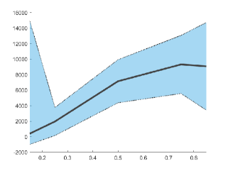
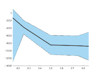
Figure 1: Heterogeneous treatment effect of JTPA

The two figures plot the 95% confidence bands for $\gamma_{4}(\tau)$ coefficient for $D_{i}\cdot W_{i,4}$ (left plot) and $\gamma_{5}(\tau)$ coefficient for $D_{i}\cdot W_{i,5}$ (right plot), where $W_{i,4}$ represents the marriage indicator (1 means being married) and $W_{i,5}$ represents the indicator of whether the person has worked for less than 13 weeks in the past year.

7 Conclusion

In this paper, we provide an alternative estimation and inference method for IVQR and related problems. This alternative approach is needed as we show that the GMM formulation of IVQR (or even a reasonable approximation) is computationally NP-hard. Our proposal focuses on obtaining good statistical properties instead of trying to improve optimization algorithms for GMM. The proposed estimator can transform, in a computationally efficient manner, an inconsistent initial estimator into one that is asymptotically equivalent to GMM. The initial estimator is obtained via MILP. We also propose a tuning-free method for estimating the Jacobian of the moment condition in a non-smooth GMM model. We illustrate our proposal in simulated and empirical data.

Appendix

Appendix A Proof of results in Section 2

Proof of Theorem 1.

We consider the following slightly easier problem.

Problem 2.

Given two numbers $\tau(0,1)$, $\eta\in(0,1/3)$ and data $\{(x_{i},z_{i},y_{i})\}_{i=1}^{n}$ with $x_{i}\in\mathbb{R}^{p}$, $z_{i}\in\mathbb{R}^{L}$ and $y_{i}$, decide whether or not the following holds:

$$\min_{\beta\in\mathbb{R}^{p}}\ \left\|\sum_{i=1}^{n}z_{i}\left(\mathbf{1}\{y_{i}-x_{i}^{\prime}\beta\leq 0\}-\tau\right)\right\|_{2}\leq\eta.$$

Problem 2 is easier than Problem 1 because any algorithm that solves Problem 1 can immediately tell us whether or not the optimal value of the objective function is smaller than $\eta$. We show that Problem 2 is NP-hard.

The rest of the proof follows the standard reduction principle. In particular, we show that the partition problem, which is one of the 21 NP-complete problems presented in Karp, (1972), can be cast as Problem 2 (or reduced to Problem 2); see (Johnson and Garey,, 1979; Sipser,, 2012) for textbook treatment on NP-completeness. Once we establish this reduction, the proof is complete because such a reduction means that any efficient algorithm solving Problem 2 is also an efficient algorithm for solving the partition problem. Since the partition problem is NP-hard, Problem 2 is also NP-hard.

Problem 3 (Partition).

Given $m$ integers $\{a_{i}\}_{i=1}^{m}$, decide whether or not the following holds: there exists a subset $B\subseteq\{1,...,m\}$ such that $\sum_{i\in B}a_{i}=\sum_{i\in\{1,...,m\}\backslash B}a_{i}$.

Now we reduce Problem 3 to Problem 2. Given $m$ integers $\{a_{i}\}_{i=1}^{m}$, we define $\tau=1/2$, $\eta=1/4$, $p=L=n=m$, $y_{i}=1/2$. Using the notation $x_{i}=(x_{i,1},...,x_{i,p})^{\prime}$ and $z_{i}=(z_{i,1},...,z_{i,p})^{\prime}$, we set

$$x_{i,j}=\begin{cases}\mathbf{1}\{i=j\}&i\leq m\\ 0&i>m\end{cases}\qquad\text{and}\qquad z_{i,j}=\begin{cases}a_{i}&i\leq m\\ 0&i>m\end{cases}\qquad\forall 1\leq i\leq m.$$

It now remains to prove the following claim.

Claim.

The answer to Problem 3 is YES if and only if the answer to Problem 2 is YES

Step 1: show the “only if” part.

Suppose that the answer to Problem 3 is YES. Then there exists $B\subset\{1,...,m\}$ such that $\sum_{i\in B}a_{i}=\sum_{i\in\{1,...,m\}\backslash B}a_{i}$. Then simply choose $\beta=(\beta_{1},\beta_{2},...,\beta_{m})^{\prime}$ with $\beta_{j}=\mathbf{1}\{j\in B\}$. Then

$$y_{i}-x_{i}^{\prime}\beta=\begin{cases}-1/2&\text{if }i\in B\\ 1/2&\text{if }i\in\{1,...,m\}\backslash B.\end{cases}$$

Then we notice that

$$\sum_{i=1}^{m}z_{i}\left(\mathbf{1}\{y_{i}-x_{i}^{\prime}\beta\leq 0\}-1/2\right)$$

$$=\sum_{i\in B}z_{i}\left(\mathbf{1}\{y_{i}-x_{i}^{\prime}\beta\leq 0\}-1/2\right)+\sum_{i\in\{1,...,m\}\backslash B}z_{i}\left(\mathbf{1}\{y_{i}-x_{i}^{\prime}\beta\leq 0\}-1/2\right)$$

$$=\sum_{i\in B}z_{i}\times(1/2)+\sum_{i\in\{1,...,m\}\backslash B}z_{i}\times(-1/2)$$

$$=\mathbf{1}_{L}\times\left(\sum_{i\in B}a_{i}-\sum_{i\in\{1,...,m\}\backslash B}a_{i}\right)\times(1/2)=0.$$

Hence, $\|\sum_{i=1}^{m}z_{i}\left(\mathbf{1}\{y_{i}-x_{i}^{\prime}\beta\leq 0\}-1/2\right)\|_{2}=0\leq\eta$, which means that the answer to Problem 2 is YES.

Step 2: show the “if” part.

Suppose that the answer to Problem 2 is YES. Then there exists $\beta\in\mathbb{R}^{m}$ such that $\left\|\sum_{i=1}^{m}z_{i}\left(\mathbf{1}\{y_{i}-x_{i}^{\prime}\beta\leq 0\}-1/2\right)\right\|_{2}\leq\eta$. Let $B=\{i:\ 1\leq i\leq m\ \text{and }x_{i}^{\prime}\beta\geq 1/2\}$.

Using the definition of $(y_{i},x_{i},z_{i})$, we know that

$$2\times\sum_{i=1}^{m}z_{i}\left(\mathbf{1}\{y_{i}-x_{i}^{\prime}\beta\leq 0\}-1/2\right)$$

$$=2\times\sum_{i\in B}z_{i}\left(\mathbf{1}\{x_{i}^{\prime}\beta\geq 1/2\}-1/2\right)+2\times\sum_{i\in\{1,...,m\}\backslash B}z_{i}\left(\mathbf{1}\{x_{i}^{\prime}\beta\geq 1/2\}-1/2\right)$$

$$=2\times\sum_{i\in B}z_{i}\times(1/2)+2\times\sum_{i\in\{1,...,m\}\backslash B}z_{i}\times(-1/2)=\sum_{i\in B}z_{i}-\sum_{i\in\{1,...,m\}\backslash B}z_{i}.$$

Since $\left\|\sum_{i=1}^{m}z_{i}\left(\mathbf{1}\{y_{i}-x_{i}^{\prime}\beta\leq 0\}-1/2\right)\right\|_{2}\leq\eta$, it follows that

$$\left\|\sum_{i\in B}z_{i}-\sum_{i\in\{1,...,m\}\backslash B}z_{i}\right\|_{2}=2\times\left\|\sum_{i=1}^{m}z_{i}\left(\mathbf{1}\{y_{i}-x_{i}^{\prime}\beta\leq 0\}-1/2\right)\right\|_{2}\leq 2\eta,$$

which means that

$$\left|\sum_{i\in B}z_{i,1}-\sum_{i\in\{1,...,m\}\backslash B}z_{i,1}\right|\leq 2\eta.$$

Since $\{z_{i,1}\}_{i=1}^{m}$ are integers $\{a_{i}\}_{i=1}^{m}$, $\sum_{i\in B}z_{i,1}-\sum_{i\in\{1,...,m\}\backslash B}z_{i,1}$ is also an integer. By $2\eta<1$, it follows that

$$\left|\sum_{i\in B}z_{i,1}-\sum_{i\in\{1,...,m\}\backslash B}z_{i,1}\right|=0,$$

which means $\sum_{i\in B}z_{i,1}=\sum_{i\in\{1,...,m\}\backslash B}z_{i,1}$. Since $z_{i,1}=a_{i}$ for $1\leq i\leq m$, the answer to Problem 3 is YES.

Notice that this same argument goes through if we replace $\|\cdot\|_{2}$-norm with $\|\cdot\|_{r}$-norm. ∎

Proof of Theorem 2.

We first introduce the following minimum unsatisfied linear relations (Min ULR).

Problem 4 (Min ULR).

Given $A\in\mathbb{Q}^{n\times p}$ and $b\in\mathbb{Q}^{n}$, find $x\in\mathbb{R}^{p}$ to minimize the number of violations in the relation $Ax>b$, i.e., number of violations in the $n$ entrywise comparisons.

The following result due to Amaldi and Kann, (1998) says that Min ULR cannot be approximated.

Theorem 7 (Theorem 2 of Amaldi and Kann, (1998)).

For any $\rho>1$, it is NP-hard to find a $\rho$-approximation for Problem 4.

We argue that Theorem 7 still holds even if we assume that $(A,b)\in(\mathbb{Q}^{n\times p}\times\mathbb{Q}^{n})\backslash\mathcal{K}$ in Problem 4, where $\mathcal{K}=\{(A,b)\in\mathbb{Q}^{n\times p}\times\mathbb{Q}^{n}:\ Ax>b\ \text{for some }x\in\mathbb{R}^{n}\}$. To see this, suppose this is not true; in other words, for some $\rho>1$, one can find a polynomial-time algorithm $\mathcal{A}$ to find a $\rho$-approximation for all instances $(A,b)\in(\mathbb{Q}^{n\times p}\times\mathbb{Q}^{n})\backslash\mathcal{K}$. Then one can use the following polynomial-time algorithm to find $\rho$-approximations for any instance $(A,b)\in\mathbb{Q}^{n\times p}\times\mathbb{Q}^{n}$. Start by running the following linear program

$$\underset{t\in\mathbb{R},\ x\in\mathbb{R}^{n}}{\text{maximize}} t\qquad\text{s.t.}\qquad A_{i}^{\prime}x\geq t+b_{i} \forall 1\leq i\leq n,$$

where $A_{i}^{\prime}$ is the $i$th row of $A$ and $b_{i}$ the $i$th component of $b$. If the solution is strictly positive, then stop; otherwise, continue by running algorithm $\mathcal{A}$. This is a contradiction to Theorem 7 unless P=NP. Therefore, Theorem 7 still holds even if we restrict Problem 4 to $(A,b)\in(\mathbb{Q}^{n\times p}\times\mathbb{Q}^{n})\backslash\mathcal{K}$. Hence, without loss of generality, we only consider instances in $(\mathbb{Q}^{n\times p}\times\mathbb{Q}^{n})\backslash\mathcal{K}$.

Now we cast Problem 4 as Problem 1. Let $(A,b)\in(\mathbb{Q}^{n\times p}\times\mathbb{Q}^{n})\backslash\mathcal{K}$ be given. We define $X=-A$ and $Y=-b$, $z_{i}=(1,...,1)^{\prime}\in\mathbb{R}^{L}$ and $\tau=1/(2n)$. Let $x_{i}^{\prime}$ denote the $i$th row of $X$ and $y_{i}$ the $i$th component of $Y$. Notice that

$$\left\|\sum_{i=1}^{n}z_{i}\left(\mathbf{1}\{y_{i}-x_{i}^{\prime}\beta\leq 0\}-\tau\right)\right\|_{2} =\sqrt{L}\left|\sum_{i=1}^{n}\left(\mathbf{1}\{y_{i}-x_{i}^{\prime}\beta\leq 0\}-\tau\right)\right|$$

$$=\sqrt{L}\left|\sum_{i=1}^{n}\mathbf{1}\{y_{i}-x_{i}^{\prime}\beta\leq 0\}-\frac{1}{2}\right|$$

$$\overset{\text{(i)}}{\geq}\frac{\sqrt{L}}{2}\sum_{i=1}^{n}\mathbf{1}\{y_{i}-x_{i}^{\prime}\beta\leq 0\},$$

where (i) follows by the fact that $(A,b)\in(\mathbb{Q}^{n\times p}\times\mathbb{Q}^{n})\backslash\mathcal{K}$ (so $\sum_{i=1}^{n}\mathbf{1}\{y_{i}-x_{i}^{\prime}\beta\leq 0\}\geq 1$). On the other hand, we clearly have

$$\left\|\sum_{i=1}^{n}Z_{i}\left(\mathbf{1}\{y_{i}-x_{i}^{\prime}\beta\leq 0\}-\tau\right)\right\|_{2} =\sqrt{L}\left|\sum_{i=1}^{n}\mathbf{1}\{y_{i}-x_{i}^{\prime}\beta\leq 0\}-\frac{1}{2}\right|$$

$$\leq\sqrt{L}\sum_{i=1}^{n}\mathbf{1}\{y_{i}-x_{i}^{\prime}\beta\leq 0\}.$$

Hence,

$$\sqrt{L}/2\leq\frac{\left\|\sum_{i=1}^{n}Z_{i}\left(\mathbf{1}\{y_{i}-x_{i}^{\prime}\beta\leq 0\}-\tau\right)\right\|_{2}}{\sum_{i=1}^{n}\mathbf{1}\{y_{i}-x_{i}^{\prime}\beta\leq 0\}}\leq\sqrt{L}.$$

Notice that $\sum_{i=1}^{n}\mathbf{1}\{y_{i}-x_{i}^{\prime}\beta\leq 0\}$ is equal to the number of violations in $Ax>b$ with $x=\beta$. The above display implies that any $\rho$-approximation for Problem 1 can be used to construct a $2\rho$-approximation for Problem 4. By Theorem 7, the desired result follows. Clearly, the above argument still holds when we replace $\|\cdot\|_{2}$ with $\|\cdot\|_{r}$. ∎

Proof of Lemma 1.

We observe that

$$\mathcal{A}(\beta,\hat{\Gamma})-\beta_{*}$$

$$=(\beta-\beta_{*})-(\hat{\Gamma}^{\prime}\hat{\Gamma})^{-1}\hat{\Gamma}^{\prime}\left[G(\beta)+n^{-1/2}H_{n}(\beta)\right]$$

$$=(\beta-\beta_{*})-(\hat{\Gamma}^{\prime}\hat{\Gamma})^{-1}\hat{\Gamma}^{\prime}\left[\Gamma_{*}(\beta-\beta_{*})+n^{-1/2}H_{n}(\beta)+\left(G(\beta)-\Gamma_{*}(\beta-\beta_{*})\right)\right]$$

$$=(I-(\hat{\Gamma}^{\prime}\hat{\Gamma})^{-1}\hat{\Gamma}^{\prime}\Gamma_{*})(\beta-\beta_{*})-(\hat{\Gamma}^{\prime}\hat{\Gamma})^{-1}\hat{\Gamma}^{\prime}\left[n^{-1/2}H_{n}(\beta)+\left(G(\beta)-\Gamma_{*}(\beta-\beta_{*})\right)\right].$$ (14)

Notice that

$$\|(I-(\hat{\Gamma}^{\prime}\hat{\Gamma})^{-1}\hat{\Gamma}^{\prime}\Gamma_{*})(\beta-\beta_{*})\|_{2}=\|(\hat{\Gamma}^{\prime}\hat{\Gamma})^{-1}\hat{\Gamma}^{\prime}(\hat{\Gamma}-\Gamma_{*})(\beta-\beta_{*})\|_{2}\leq\|(\hat{\Gamma}^{\prime}\hat{\Gamma})^{-1}\hat{\Gamma}\|\times\|\hat{\Gamma}-\Gamma_{*}\|\times\|\beta-\beta_{*}\|_{2}.$$

Since $\|G(\beta)-\Gamma_{*}(\beta-\beta_{*})\|_{2}\leq c\|\beta-\beta_{*}\|_{2}^{2}$ and $\|H_{n}(\beta)\|_{2}\leq\sup_{v\in\mathcal{B}_{0}}\|H_{n}(v)\|_{2}$, the desired result follows. ∎

Proof of Theorem 3.

First notice that the assumption of $c_{3}^{-1/2}c_{5}n^{-1/2}\leq(1-\rho_{*})c_{1}$ means that $\rho_{*}\leq 1-n^{-1/2}c_{1}^{-1}c_{3}^{-1/2}c_{5}<1$.

Notice that $\|(\hat{\Gamma}^{\prime}\hat{\Gamma})^{-1}\hat{\Gamma}^{\prime}\|_{2}=1/\sqrt{\lambda_{\min}(\hat{\Gamma}^{\prime}\hat{\Gamma})}\leq c_{3}^{-1/2}$. Then by Lemma 1, we have that

$$\|\hat{\beta}_{(1)}-\beta_{*}\|_{2} \leq c_{3}^{-1/2}c_{2}\|\bar{\beta}-\beta_{*}\|_{2}+c_{3}^{-1/2}\left(n^{-1/2}c_{5}+c_{4}\|\bar{\beta}-\beta_{*}\|_{2}^{2}\right)$$

$$\leq c_{3}^{-1/2}c_{2}\|\bar{\beta}-\beta_{*}\|_{2}+c_{3}^{-1/2}\left(n^{-1/2}c_{5}+c_{1}c_{4}\|\bar{\beta}-\beta_{*}\|_{2}\right)$$

$$=\rho_{*}\|\bar{\beta}-\beta_{*}\|_{2}+c_{3}^{-1/2}c_{5}n^{-1/2}.$$

By the assumption of $c_{5}\leq\sqrt{n}c_{1}c_{3}^{1/2}(1-\rho_{*})$, we have that $c_{3}^{-1/2}c_{5}n^{-1/2}\leq(1-\rho_{*})c_{1}$. Hence, $\|\hat{\beta}_{(1)}-\beta_{*}\|_{2}\leq c_{1}$. By induction, we have that $\|\hat{\beta}_{(k)}-\beta_{*}\|_{2}\leq c_{1}$ for any $k\geq 1$.

We now notice that the same computation as above yields that for any $k\geq 1$,

$$\|\hat{\beta}_{(k)}-\beta_{*}\|_{2}\leq\rho_{*}\|\hat{\beta}_{(k-1)}-\beta_{*}\|_{2}+c_{3}^{-1/2}c_{5}n^{-1/2}.$$

Thus, the desired result follows by a simple induction argument. ∎

Proof of Corollary 1.

We shall use the notations from the statement of Theorem 3. We also write $\hat{\beta}_{(k)}=\mathcal{A}_{k}(\bar{\beta},\hat{\Gamma})$. Since Theorem 3 is a finite-sample result that holds with probability one, we can define $c_{1},...,c_{5}$ to be random or non-random quantities. Set $c_{1}=\min\{\sqrt{\kappa_{3}}/(8\kappa_{1}),\ \kappa_{2}\}$, $c_{2}=\sqrt{\kappa_{3}}/8$, $c_{3}=\kappa_{3}/4$, $c_{4}=\kappa_{1}$ and $c_{5}=\sup_{\|v-\beta_{*}\|_{2}\leq\kappa_{2}}\|H_{n}(v)\|_{2}$. Let $\rho_{*}=c_{3}^{-1/2}(c_{2}+c_{1}c_{4})\leq 1/2$. Define the event

$$\mathcal{M}=\left\{\|\bar{\beta}-\beta_{*}\|_{2}\leq c_{1}\right\}\bigcap\left\{\|\hat{\Gamma}-\Gamma_{*}\|\leq c_{2}\right\}\bigcap\left\{\sup_{\|v-\beta_{*}\|_{2}\leq\kappa_{2}}\|H_{n}(v)\|_{2}\leq\sqrt{n}\kappa_{3}/(32\kappa_{1})\right\}.$$

Now we verify the conditions of Theorem 3 on the event $\mathcal{M}$.

Let $\sigma_{\min}(\cdot)$ and $\sigma_{\max}(\cdot)$ denote the minimum and the maximum singular values, respectively. Then $\sigma_{\min}(\Gamma_{*})\geq\sqrt{\kappa_{3}}$. Recall the elementary inequality of $\sigma_{\min}(A)+\sigma_{\max}(B)\geq\sigma_{\min}(A+B)$ for any matrices $A,B$. Hence, on the event $\mathcal{M}$,

$$\sqrt{\lambda_{\min}(\hat{\Gamma}^{\prime}\hat{\Gamma})}=\sigma_{\min}(\hat{\Gamma})\geq\sigma_{\min}(\Gamma_{*})-\sigma_{\max}(\Gamma_{*}-\hat{\Gamma})=\sqrt{\kappa_{3}}-\|\hat{\Gamma}-\Gamma\|\geq\sqrt{\kappa_{3}}-c_{2}=7\sqrt{\kappa_{3}}/8.$$

Therefore, on the event $\mathcal{M}$, $\lambda_{\min}(\hat{\Gamma}^{\prime}\hat{\Gamma})\geq\kappa_{3}(7/8)^{2}>c_{3}$. Notice that on the event $\mathcal{M}$, $c_{5}\leq c_{1}c_{3}^{1/2}\sqrt{n}(1-\rho_{*})$ by definition since $\rho_{*}\leq 1/2$ and $c_{1}\leq\sqrt{\kappa_{3}}/(8\kappa_{1})$. Therefore, all the conditions of Theorem 3 are satisfied on the event $\mathcal{M}$. It follows by Theorem 3 that on the event $\mathcal{M}$, for any $K\geq 1$,

$$\|\hat{\beta}_{(K)}-\beta_{*}\|_{2}\leq 2^{-K}c_{1}+2n^{-1/2}c_{3}^{-1/2}c_{5}\leq 2^{-K}\kappa_{2}+2n^{-1/2}c_{3}^{-1/2}c_{5}.$$

Notice that $1/(2\log 2)<2$. Thus, for any $K\geq 2\log n$, we have that $2^{-K}\leq 2^{-2\log n}\leq 2^{-(\log n)/(2\log 2)}=n^{-1/2}$. Hence, on the event $\mathcal{M}$, for any $K\geq 2\log n$, we have

$$\|\hat{\beta}_{(K)}-\beta_{*}\|_{2}\leq n^{-1/2}\kappa_{2}+4n^{-1/2}\kappa_{3}^{-1/2}c_{5}.$$

Thus, $P(\sup_{K\geq 2\log n}\|\hat{\beta}_{(K)}-\beta_{*}\|_{2}\leq n^{-1/2}\kappa_{2}+4n^{-1/2}\kappa_{3}^{-1/2}c_{5})\geq P(\mathcal{M})$. Since $\sup_{\|v-\beta_{*}\|_{2}\leq\kappa_{2}}\|H_{n}(v)\|_{2}=O_{P}(1)$, the proof is complete. ∎

Proof of Theorem 4.

We inherit all the notations and definitions from the proof of Corollary 1. Since $\varepsilon=\varepsilon_{n}=o(1)$, we can assume $\varepsilon\in(0,\sqrt{\kappa_{3}}/8)$. We now fix $K$, $\beta$ and $\Gamma$ such that $K\geq 1+2\log n$, $\|\beta-\beta_{*}\|_{2}\leq A$ and $\|\Gamma-\Gamma_{*}\|\leq\varepsilon$.

Let $K_{0}=K-1$. In the proof of Corollary 1, we have showed that on the event $\mathcal{M}$,

$$\|\mathcal{A}_{K_{0}}(\beta,\Gamma)-\beta_{*}\|_{2}\leq n^{-1/2}\kappa_{2}+4n^{-1/2}\kappa_{3}^{-1/2}\sup_{\|v-\beta_{*}\|_{2}\leq\kappa_{2}}\|H_{n}(v)\|_{2},$$

where the event $\mathcal{M}$ is defined by

$$\mathcal{M}=\left\{\sup_{\|v-\beta_{*}\|_{2}\leq\kappa_{2}}\|H_{n}(v)\|_{2}\leq\sqrt{n}\kappa_{3}/(32\kappa_{1})\right\}.$$

Define $\eta_{0}=1-P(\mathcal{M})$. Fix an arbitrary $\eta\in(0,1)$, we find a constant $M_{\eta}>0$ such that $P(\sup_{\|v-\beta_{*}\|_{2}\leq\kappa_{2}}\|H_{n}(v)\|_{2}>M_{\eta})\leq\eta$. This is possible since we assume $\sup_{\|v-\beta_{*}\|_{2}\leq\kappa_{2}}\|H_{n}(v)\|_{2}=O_{P}(1)$. Now we define the event $\bar{\mathcal{M}}=\left\{\sup_{\|v-\beta_{*}\|_{2}\leq\kappa_{2}}\|H_{n}(v)\|_{2}\leq\min\{M_{\eta},\ \sqrt{n}\kappa_{3}/(32\kappa_{1})\}\right\}$. Notice that $P(\bar{\mathcal{M}})\geq 1-\max\{\eta_{0},\ \eta\}$ and $\bar{\mathcal{M}}\subseteq\mathcal{M}$. Therefore, on the event $\bar{\mathcal{M}}$, we have

$$\|\mathcal{A}_{K_{0}}(\beta,\Gamma)-\beta_{*}\|_{2}\leq n^{-1/2}C_{\eta},$$

where $C_{\eta}=\kappa_{2}+4\kappa_{3}^{-1/2}\min\{M_{\eta},\ \sqrt{n}\kappa_{3}/(32\kappa_{1})\}$.

Now we recall the basic decomposition (14) from the proof of Lemma 1:

$$\mathcal{A}_{K}(\beta,\Gamma)-\beta_{*}$$

$$=\mathcal{A}(\mathcal{A}_{K_{0}}(\beta,\Gamma),\Gamma)-\beta_{*}$$

$$=(I-(\Gamma^{\prime}\Gamma)^{-1}\Gamma^{\prime}\Gamma_{*})(\mathcal{A}_{K_{0}}(\beta,\Gamma)-\beta_{*})$$

$$\qquad-(\Gamma^{\prime}\Gamma)^{-1}\Gamma^{\prime}\left[n^{-1/2}H_{n}(\mathcal{A}_{K_{0}}(\beta,\Gamma))+\left(G(\mathcal{A}_{K_{0}}(\beta,\Gamma))-\Gamma_{*}(\mathcal{A}_{K_{0}}(\beta,\Gamma)-\beta_{*})\right)\right].$$ (15)

By the proof of Theorem 3, we have that $\|\mathcal{A}_{K_{0}}(\beta,\Gamma)-\beta_{*}\|_{2}\leq c_{1}$, where $c_{1}=\min\{\sqrt{\kappa_{3}}/(8\kappa_{1}),\ \kappa_{2}\}$ (defined in the proof of Corollary 1). Also in the proof of Corollary 1, we have that on the event $\mathcal{M}$, $\lambda_{\min}(\Gamma^{\prime}\Gamma)\geq\kappa_{3}(7/8)^{2}$.

Since $I-(\Gamma^{\prime}\Gamma)^{-1}\Gamma^{\prime}\Gamma_{*}=(\Gamma^{\prime}\Gamma)^{-1}\Gamma^{\prime}(\Gamma-\Gamma_{*})$ and $\|(\Gamma^{\prime}\Gamma)^{-1}\Gamma^{\prime}\|=1/\sqrt{\lambda_{\min}(\Gamma^{\prime}\Gamma)}$, we have that on the event $\bar{\mathcal{M}}$,

$$\|\mathcal{A}_{K}(\beta,\Gamma)-\beta_{*}+n^{-1/2}(\Gamma^{\prime}\Gamma)^{-1}\Gamma^{\prime}H_{n}(\beta_{*})\|_{2}$$

$$\leq\varepsilon\|(\Gamma^{\prime}\Gamma)^{-1}\Gamma^{\prime}\|\cdot\|\mathcal{A}_{K_{0}}(\beta,\Gamma)-\beta_{*}\|_{2}+\|(\Gamma^{\prime}\Gamma)^{-1}\Gamma^{\prime}\|\cdot n^{-1/2}\|H_{n}(\mathcal{A}_{K_{0}}(\beta,\Gamma))-H_{n}(\beta_{*})\|_{2}$$

$$\qquad+\kappa_{1}\|(\Gamma^{\prime}\Gamma)^{-1}\Gamma^{\prime}\|\cdot\|\mathcal{A}_{K_{0}}(\beta,\Gamma)-\beta_{*}\|_{2}^{2}$$

$$\leq\frac{8}{7}\kappa_{3}^{-1/2}\varepsilon\cdot\|\mathcal{A}_{K_{0}}(\beta,\Gamma)-\beta_{*}\|_{2}+\frac{8}{7}\kappa_{3}^{-1/2}\cdot n^{-1/2}\|H_{n}(\mathcal{A}_{K_{0}}(\beta,\Gamma))-H_{n}(\beta_{*})\|_{2}$$

$$\qquad+\frac{8}{7}\kappa_{3}^{-1/2}\kappa_{1}\cdot\|\mathcal{A}_{K_{0}}(\beta,\Gamma)-\beta_{*}\|_{2}^{2}$$

$$\leq\frac{8}{7}\kappa_{3}^{-1/2}\varepsilon n^{-1/2}C_{\eta}+\frac{8}{7}\kappa_{3}^{-1/2}\cdot n^{-1/2}\sup_{\|v\|_{2}\leq C_{\eta}}\|H_{n}(\beta_{*}+n^{-1/2}v)-H_{n}(\beta_{*})\|_{2}+\frac{8}{7}\kappa_{3}^{-1/2}\kappa_{1}n^{-1}C_{\eta}^{2}.$$

By the continuity of $\Gamma\mapsto(\Gamma^{\prime}\Gamma)^{-1}\Gamma^{\prime}$, it is not hard to see that there exists a constant $D>0$ depending only on $\kappa_{3}$ such that $\|(\Gamma^{\prime}\Gamma)^{-1}\Gamma^{\prime}-(\Gamma_{*}^{\prime}\Gamma_{*})^{-1}\Gamma_{*}^{\prime}\|\leq D\|\Gamma-\Gamma_{*}\|$ for small enough $\varepsilon$. Therefore,

$$\left\|\left[(\Gamma^{\prime}\Gamma)^{-1}\Gamma^{\prime}-(\Gamma_{*}^{\prime}\Gamma_{*})^{-1}\Gamma_{*}^{\prime}\right]H_{n}(\beta_{*})\right\|_{2}\leq D\varepsilon\|H_{n}(\beta_{*})\|_{2}.$$

The above two displays imply that on the even $\bar{\mathcal{M}}$,

$$\|\mathcal{A}_{K}(\beta,\Gamma)-\beta_{*}+n^{-1/2}(\Gamma_{*}^{\prime}\Gamma_{*})^{-1}\Gamma_{*}^{\prime}H_{n}(\beta_{*})\|_{2}\\ \leq Dn^{-1/2}\varepsilon\|H_{n}(\beta_{*})\|_{2}+\frac{8}{7}\kappa_{3}^{-1/2}\varepsilon n^{-1/2}C_{\eta}+\frac{8}{7}\kappa_{3}^{-1/2}\cdot n^{-1/2}\sup_{\|v\|_{2}\leq C_{\eta}}\|H_{n}(\beta_{*}+n^{-1/2}v)-H_{n}(\beta_{*})\|_{2}\\ +\frac{8}{7}\kappa_{3}^{-1/2}\kappa_{1}n^{-1}C_{\eta}^{2}.$$

Since the above argument holds for any sample path on $\bar{\mathcal{M}}$ and for any $(\beta,\Gamma)$, we have on the even $\bar{\mathcal{M}}$,

$$\sup_{\|\beta-\beta_{*}\|_{2}\leq A,\ \|\Gamma-\Gamma_{*}\|\leq\varepsilon}\|\mathcal{A}_{K}(\beta,\Gamma)-\beta_{*}+n^{-1/2}(\Gamma_{*}^{\prime}\Gamma_{*})^{-1}\Gamma_{*}^{\prime}H_{n}(\beta_{*})\|_{2}\\ \leq Dn^{-1/2}\varepsilon\|H_{n}(\beta_{*})\|_{2}+D_{1}\varepsilon n^{-1/2}+\frac{8}{7}\kappa_{3}^{-1/2}\cdot n^{-1/2}\sup_{\|v\|_{2}\leq C_{\eta}}\|H_{n}(\beta_{*}+n^{-1/2}v)-H_{n}(\beta_{*})\|_{2}\\ +n^{-1}D_{2},$$

where $D_{1}=\frac{8}{7}\kappa_{3}^{-1/2}C_{\eta}$ and $D_{2}=\frac{8}{7}\kappa_{3}^{-1/2}\kappa_{1}C_{\eta}^{2}$.

Since $\eta_{0}=o(1)$, it follows that

$$P\Biggl{(}\sup_{\|\beta-\beta_{*}\|_{2}\leq A,\ \|\Gamma-\Gamma_{*}\|\leq\varepsilon}\|\mathcal{A}_{K}(\beta,\Gamma)-\beta_{*}+n^{-1/2}(\Gamma_{*}^{\prime}\Gamma_{*})^{-1}\Gamma_{*}^{\prime}H_{n}(\beta_{*})\|_{2}$$

$$\qquad>Dn^{-1/2}\varepsilon\|H_{n}(\beta_{*})\|_{2}+D_{1}\varepsilon n^{-1/2}+\frac{8}{7}\kappa_{3}^{-1/2}\cdot n^{-1/2}\sup_{\|v\|_{2}\leq C_{\eta}}\|H_{n}(\beta_{*}+n^{-1/2}v)-H_{n}(\beta_{*})\|_{2}+n^{-1}D_{2}\Biggr{)}$$

$$\leq P(\bar{\mathcal{M}}^{c})\leq\max\{\eta_{0},\ \eta\}\leq o(1)+\eta.$$

Since $\eta>0$ is arbitrary and $\sup_{\|v\|_{2}\leq C}\|H_{n}(\beta_{*}+n^{-1/2}v)-H_{n}(\beta_{*})\|_{2}=o_{P}(1)$ for any $C>0$, the desired result follows. ∎

Appendix B Proof of results in Section 3

Proof of Lemma 2.

Notice that by Taylor’s theorem, we have

$$G_{n}^{*}(b_{*}) =n^{-1/2}H_{n}^{*}(b_{*})+G_{n}(b_{*})$$

$$=n^{-1/2}H_{n}^{*}(b_{*})+n^{-1/2}H_{n}(b_{*})+G(b_{*})$$

$$=n^{-1/2}H_{n}^{*}(b_{*})+n^{-1/2}H_{n}(b_{*})+G(b_{0})+\Gamma_{0}(b_{*}-b_{0})+a_{n}^{*}(b_{*}-b_{0})^{2},$$

for some random variable $a_{n}^{*}$ with $|a_{n}^{*}|\leq\sup_{\beta}|d^{2}G(\beta)/d\beta^{2}|$. On the other hand,

$$G_{n}(b_{0})=n^{-1/2}H_{n}(b_{0})+G(b_{0}).$$

Since $G_{n}^{*}(b_{*})=G_{n}(b_{0})$, we have that

$$n^{-1/2}H_{n}^{*}(b_{*})+n^{-1/2}H_{n}(b_{*})+G(b_{0})+\Gamma_{0}(b_{*}-b_{0})+a_{n}^{*}(b_{*}-b_{0})^{2}=n^{-1/2}H_{n}(b_{0})+G(b_{0}).$$

The desired result follows. ∎

Proof of Theorem 5.

Let $\delta=b_{*}-b_{0}$. By Lemma 2, we have

$$\hat{\Gamma}_{0}-\Gamma_{0}=\frac{E\left(-n^{-1/2}H_{n}^{*}(b_{*})\delta\mid\mathcal{F}\right)}{E(\delta^{2}\mid\mathcal{F})}-\Gamma_{0}=\frac{E\left((\Gamma_{0}\delta+\varepsilon)\delta\mid\mathcal{F}\right)}{E(\delta^{2}\mid\mathcal{F})}-\Gamma_{0}=\frac{E\left(\delta\varepsilon\mid\mathcal{F}\right)}{E(\delta^{2}\mid\mathcal{F})},$$ (16)

where $\varepsilon=a_{n}^{*}\delta^{2}+n^{-1/2}B_{n}$ with $B_{n}=H_{n}(b_{*})-H_{n}(b_{0})$. Fix an arbitrary number $\eta\in(0,1)$.

By the assumption, there exists a constant $C>0$ such that with probability at least $1-\eta$, (1) $E\left(\sup_{\beta}|H_{n}^{*}(\beta)|\mid\mathcal{F}\right)$ and $\sup_{\beta}|H_{n}(\beta)|$ are bounded by $C$ and (2) $\sup_{|x-y|\leq n^{-1/2}t}|H_{n}(x)-H_{n}(y)|\leq\eta$. We define the following event

$$\mathcal{M}=\left\{\sup_{|x-y|\leq n^{-1/2}\eta^{-1}}|H_{n}(x)-H_{n}(y)|\leq\eta\right\}\bigcap\left\{E\left(\sup_{\beta}|H_{n}^{*}(\beta)|^{4}\mid\mathcal{F}\right)\leq C\right\}\\ \bigcap\left\{\sup_{\beta}|H_{n}(\beta)|\leq C\right\}\bigcap\left\{E\left(\sup_{|x-y|\leq n^{-1/2}\eta^{-1}}|H_{n}^{*}(x)-H_{n}^{*}(y)|^{4}\mid\mathcal{F}\right)\leq C\right\}\\ \bigcap\left\{\rho_{2}<|\Gamma_{0}|<\rho_{3}\right\}\bigcap\left\{E\left((H_{n}^{*}(b_{0}))^{2}\mid\mathcal{F}\right)\geq\rho_{4}\right\}.$$

By assumption, $P(\mathcal{M})=1-\eta-o(1)$. Now we proceed in three steps, in which we first characterize $\delta$ and then provide bounds for $E(\delta\varepsilon\mid\mathcal{F})$ and $E(\delta^{2}\mid\mathcal{F})$.

Step 1: provide preliminary bounds for $\delta$.

We first characterize the size of $\delta$. By Lemma 2, $-n^{-1/2}H_{n}^{*}(b_{*})=\Gamma_{0}\delta+a_{n}^{*}\delta^{2}+n^{-1/2}B_{n}$. We rearrange the terms and obtain

$$\frac{a_{n}^{*}}{\Gamma_{0}}\delta^{2}+\delta+\frac{n^{-1/2}(H_{n}^{*}(b_{*})+B_{n})}{\Gamma_{0}}=0.$$

By the quadratic formula, we have $2a_{n}^{*}\Gamma_{0}^{-1}\delta\in\{W_{1},W_{2}\}$, where $W_{1}=\sqrt{1-4Q_{n}}-1$, $W_{2}=-\sqrt{1-4Q_{n}}-1$ and $Q_{n}=n^{-1/2}a_{n}^{*}(H_{n}^{*}(b_{*})+B_{n})\Gamma_{0}^{-2}$. Notice that $1\leq|W_{2}|\leq 2$ and

$$|W_{1}|=\frac{\left|\sqrt{1-4Q_{n}}-1\right|}{1}=\frac{\left|-4Q_{n}\right|}{\sqrt{1-4Q_{n}}+1}\leq 4|Q_{n}|.$$ (17)

On the event $\mathcal{M}$, we have

$$E\left(|Q_{n}|^{3}\mid\mathcal{F}\right) \leq\left(n^{-1/2}\rho_{1}\rho_{2}^{-2}\right)^{3}E\left([|H_{n}^{*}(b_{*})|+2C]^{3}\mid\mathcal{F}\right)$$

$$\overset{\text{(i)}}{\leq}4\left(n^{-1/2}\rho_{1}\rho_{2}^{-2}\right)^{3}E\left(|H_{n}^{*}(b_{*})|^{3}+8C^{3}\mid\mathcal{F}\right)$$

$$\leq 4\left(n^{-1/2}\rho_{1}\rho_{2}^{-2}\right)^{3}\left(C^{3}+8C^{3}\right)=n^{-3/2}\kappa$$

with $\kappa=36\rho_{1}^{3}\rho_{2}^{-6}$, where (i) follows by the elementary inequality $(a+b)^{3}\leq 4(a^{3}+b^{3})$. Since $b_{*}$ is chosen to be the closest solution to $b_{0}$, it follows that $2a_{n}^{*}\Gamma_{0}^{-1}\delta=W_{2}$ only if $|W_{2}|\leq|W_{1}|$. Due to $|W_{2}|\geq 1$ and (17), $|W_{2}|\leq|W_{1}|$ implies $|Q_{n}|\geq 1/4$. Therefore,

$$P\left(2a_{n}^{*}\Gamma_{0}^{-1}\delta\neq W_{1}\mid\mathcal{F}\right)\leq P\left(|Q_{n}|\geq 1/4\mid\mathcal{F}\right)=P\left(|Q_{n}|^{3}\geq 1/64\mid\mathcal{F}\right)\\ \leq 64E\left(|Q_{n}|^{3}\mid\mathcal{F}\right)\leq 64\kappa n^{-3/2}.$$ (18)

By (17) and the definition of $Q_{n}$, we have that

$$|\delta|\mathbf{1}\{2a_{n}^{*}\Gamma_{0}^{-1}\delta=W_{1}\} =\left|\frac{W_{1}}{2a_{n}^{*}\Gamma_{0}^{-1}}\right|\mathbf{1}\{2a_{n}^{*}\Gamma_{0}^{-1}\delta=W_{1}\}$$

$$\leq\left|\frac{2Q_{n}}{a_{n}^{*}\Gamma_{0}^{-1}}\right|\mathbf{1}\{2a_{n}^{*}\Gamma_{0}^{-1}\delta=W_{1}\}$$

$$\leq 2n^{-1/2}\rho_{3}\left|H_{n}^{*}(b_{*})+B_{n}\right|\mathbf{1}\{2a_{n}^{*}\Gamma_{0}^{-1}\delta=W_{1}\}.$$ (19)

By construction, $|\delta|\leq\bar{C}$. Thus, for any $r\in[1,4]$, we observe that

$$E(|\delta|^{r}\mid\mathcal{F})$$

$$=E(|\delta|^{r}\mathbf{1}\{2a_{n}^{*}\Gamma_{0}^{-1}\delta=W_{1}\}\mid\mathcal{F})+E(|\delta|^{r}\mathbf{1}\{2a_{n}^{*}\Gamma_{0}^{-1}\delta\neq W_{1}\}\mid\mathcal{F})$$

$$\leq 2^{r}n^{-r/2}\rho_{3}^{r}E\left(\left(|H_{n}^{*}(b_{*})|+2C\right)^{r}\times\mathbf{1}\{2a_{n}^{*}\Gamma_{0}^{-1}\delta=W_{1}\}\mid\mathcal{F}\right)+\bar{C}^{r}P\left(2a_{n}^{*}\Gamma_{0}^{-1}\delta\neq W_{1}\mid\mathcal{F}\right)$$

$$\overset{\text{(i)}}{\leq}2^{2r-1}n^{-r/2}\rho_{3}^{r}E\left(\left(|H_{n}^{*}(b_{*})|^{r}+2^{r}C^{r}\right)\times\mathbf{1}\{2a_{n}^{*}\Gamma_{0}^{-1}\delta=W_{1}\}\mid\mathcal{F}\right)+\bar{C}^{r}P\left(2a_{n}^{*}\Gamma_{0}^{-1}\delta\neq W_{1}\mid\mathcal{F}\right)$$

$$\overset{\text{(ii)}}{\leq}2^{2r-1}n^{-r/2}\rho_{3}^{r}C^{r}(1+2^{r})+\bar{C}^{r}\times 64\kappa n^{-3/2},$$

where (i) follows by the elementary inequality $(a+b)^{r}\leq 2^{r-1}(a^{r}+b^{r})$ for $a,b\geq 0$ and (ii) follows by the definition of $\mathcal{M}$ and (18). Therefore, there exists a constant $C_{0}>0$ such that

$$E(|\delta|^{r}\mid\mathcal{F})\leq C_{0}\left(n^{-r/2}+n^{-3/2}\right)\qquad\forall r\in[1,4].$$ (20)

Step 2: derive a lower bound for $E(\delta^{2}\mid\mathcal{F})$.

By (20), we have

$$P\left(|\delta|>n^{-1/2}\eta^{-1}\mid\mathcal{F}\right)\leq n^{1/2}\eta E(|\delta|\mid\mathcal{F})\leq C_{0}\left(1+n^{-1}\right)\eta\leq 2C_{0}\eta.$$ (21)

Clearly, $|B_{n}|\leq 2C$ on the event $\mathcal{M}$. Thus,

$$E\left(B_{n}^{2}\mid\mathcal{F}\right) =E\left(B_{n}^{2}\mathbf{1}\{|\delta|>n^{-1/2}\eta^{-1}\}\mid\mathcal{F}\right)+E\left(B_{n}^{2}\mathbf{1}\{|\delta|\leq n^{-1/2}\eta^{-1}\}\mid\mathcal{F}\right)$$

$$\leq 4C^{2}P\left(|\delta|>n^{-1/2}\eta^{-1}\mid\mathcal{F}\right)+E\left(B_{n}^{2}\mathbf{1}\{|\delta|\leq n^{-1/2}\eta^{-1}\}\mid\mathcal{F}\right)$$

$$\overset{\text{(i)}}{\leq}4C^{2}P\left(|\delta|>n^{-1/2}\eta^{-1}\mid\mathcal{F}\right)+\eta^{2}E\left(\mathbf{1}\{|\delta|\leq n^{-1/2}\eta^{-1}\}\mid\mathcal{F}\right)$$

$$\leq 8C^{2}C_{0}\eta+\eta^{2},$$ (22)

where (i) follows by the fact that on the event $\mathcal{M}\bigcap\{|\delta|\leq n^{-1/2}\eta^{-1}\}$, $|B_{n}|\leq\sup_{|x-y|\leq n^{-1/2}\eta^{-1}}|H_{n}(x)-H_{n}(y)|\leq\eta$. Similarly, we have

$$E\left((H_{n}^{*}(b_{*})-H_{n}^{*}(b_{0}))^{2}\mid\mathcal{F}\right)$$

$$=E\left((H_{n}^{*}(b_{*})-H_{n}^{*}(b_{0}))^{2}\mathbf{1}\{|\delta|>n^{-1/2}\eta^{-1}\}\mid\mathcal{F}\right)$$

$$\qquad\qquad+E\left((H_{n}^{*}(b_{*})-H_{n}^{*}(b_{0}))^{2}\mathbf{1}\{|\delta|\leq n^{-1/2}\eta^{-1}\}\mid\mathcal{F}\right)$$

$$\overset{\text{(i)}}{\leq}\sqrt{E\left((H_{n}^{*}(b_{*})-H_{n}^{*}(b_{0}))^{4}\mid\mathcal{F}\right)\times P\left(|\delta|>n^{-1/2}\eta^{-1}\mid\mathcal{F}\right)}$$

$$\qquad\qquad+E\left((H_{n}^{*}(b_{*})-H_{n}^{*}(b_{0}))^{2}\mathbf{1}\{|\delta|\leq n^{-1/2}\eta^{-1}\}\mid\mathcal{F}\right)$$

$$\overset{\text{(ii)}}{\leq}\sqrt{8E\left(\left[|H_{n}^{*}(b_{*})|^{4}+|H_{n}^{*}(b_{0})|^{4}\right]\mid\mathcal{F}\right)\times P\left(|\delta|>n^{-1/2}\eta^{-1}\mid\mathcal{F}\right)}$$

$$\qquad\qquad+E\left((H_{n}^{*}(b_{*})-H_{n}^{*}(b_{0}))^{2}\mathbf{1}\{|\delta|\leq n^{-1/2}\eta^{-1}\}\mid\mathcal{F}\right)$$

$$\overset{\text{(iii)}}{\leq}\sqrt{16C\times 2C_{0}\eta}+E\left((H_{n}^{*}(b_{*})-H_{n}^{*}(b_{0}))^{2}\mathbf{1}\{|\delta|\leq n^{-1/2}\eta^{-1}\}\mid\mathcal{F}\right)$$

$$\overset{\text{(iv)}}{\leq}\sqrt{32CC_{0}\eta}+E\left(\eta^{2}\mathbf{1}\{|\delta|\leq n^{-1/2}\eta^{-1}\}\mid\mathcal{F}\right)$$

$$\leq\sqrt{32CC_{0}\eta}+\eta^{2},$$ (23)

where (i) follows by Cauchy-Schwarz inequality, (ii) follows by the elementary inequality $(a-b)^{4}\leq(|a|+|b|)^{4}\leq 8(|a|^{4}+|b|^{4})$ for $a,b\in\mathbb{R}$, (iii) follows by (21) and the definition of $\mathcal{M}$ and finally (iv) follows by the fact that on the event $\mathcal{M}\bigcap\{|\delta|\leq n^{-1/2}\eta^{-1}\}$,

$$\left|H_{n}^{*}(b_{*})-H_{n}^{*}(b_{0})\right|\leq\sup_{|x-y|\leq n^{-1/2}\eta^{-1}}\left|H_{n}^{*}(x)-H_{n}^{*}(y)\right|\leq\eta.$$

By (22) and (23), there exists a constant $C_{1}>0$ independent of $\eta$ such that

$$\max\left\{E\left((H_{n}^{*}(b_{*})-H_{n}^{*}(b_{0}))^{2}\mid\mathcal{F}\right),\ E\left(B_{n}^{2}\mid\mathcal{F}\right)\right\}\leq C_{1}^{2}\sqrt{\eta}.$$ (24)

We notice that

$$E(\delta^{2}\mid\mathcal{F}) \geq E(\delta^{2}\mathbf{1}\{2a_{n}^{*}\Gamma_{0}^{-1}\delta=W_{1}\}\mid\mathcal{F})$$

$$=E\left(\frac{W_{1}^{2}}{4(a_{n}^{*})^{2}\Gamma_{0}^{-2}}\times\mathbf{1}\{2a_{n}^{*}\Gamma_{0}^{-1}\delta=W_{1}\}\mid\mathcal{F}\right)$$

$$\geq E\left(\frac{4Q_{n}^{2}}{4(a_{n}^{*})^{2}\Gamma_{0}^{-2}}\times\mathbf{1}\{2a_{n}^{*}\Gamma_{0}^{-1}\delta=W_{1}\}\mid\mathcal{F}\right)$$

$$=\Gamma_{0}^{2}n^{-1}E\left((H_{n}^{*}(b_{*})+B_{n})^{2}\times\mathbf{1}\{2a_{n}^{*}\Gamma_{0}^{-1}\delta=W_{1}\}\mid\mathcal{F}\right)$$

$$\geq\rho_{2}^{2}n^{-1}E\left((H_{n}^{*}(b_{*})+B_{n})^{2}\times\mathbf{1}\{2a_{n}^{*}\Gamma_{0}^{-1}\delta=W_{1}\}\mid\mathcal{F}\right).$$ (25)

For a random variable $R$, we can verify that $\|R\|:=\sqrt{E(R^{2}\times\mathbf{1}\{2a_{n}^{*}\Gamma_{0}^{-1}\delta=W_{1}\}\mid\mathcal{F})}$ is a semi-norm and we hence can apply the triangular inequality $\|R^{(1)}+R^{(2)}+R^{(3)}\|\geq\|R^{(1)}\|-\|R^{(2)}\|-\|R^{(3)}\|$ for any norm. Therefore, we notice that

$$\sqrt{E\left((H_{n}^{*}(b_{*})+B_{n})^{2}\times\mathbf{1}\{2a_{n}^{*}\Gamma_{0}^{-1}\delta=W_{1}\}\mid\mathcal{F}\right)}$$

$$=\sqrt{E\left(\left[H_{n}^{*}(b_{0})+(H_{n}^{*}(b_{*})-H_{n}^{*}(b_{0}))+B_{n}\right]^{2}\times\mathbf{1}\{2a_{n}^{*}\Gamma_{0}^{-1}\delta=W_{1}\}\mid\mathcal{F}\right)}$$

$$\geq\sqrt{E\left((H_{n}^{*}(b_{0}))^{2}\times\mathbf{1}\{2a_{n}^{*}\Gamma_{0}^{-1}\delta=W_{1}\}\mid\mathcal{F}\right)}$$

$$\qquad-\sqrt{E\left((H_{n}^{*}(b_{*})-H_{n}^{*}(b_{0}))^{2}\times\mathbf{1}\{2a_{n}^{*}\Gamma_{0}^{-1}\delta=W_{1}\}\mid\mathcal{F}\right)}$$

$$\qquad-\sqrt{E\left(B_{n}^{2}\times\mathbf{1}\{2a_{n}^{*}\Gamma_{0}^{-1}\delta=W_{1}\}\mid\mathcal{F}\right)}$$

$$\geq\sqrt{E\left((H_{n}^{*}(b_{0}))^{2}\times\mathbf{1}\{2a_{n}^{*}\Gamma_{0}^{-1}\delta=W_{1}\}\mid\mathcal{F}\right)}-\sqrt{E\left((H_{n}^{*}(b_{*})-H_{n}^{*}(b_{0}))^{2}\mid\mathcal{F}\right)}-\sqrt{E\left(B_{n}^{2}\mid\mathcal{F}\right)}$$

$$\overset{\text{(i)}}{\geq}\sqrt{E\left((H_{n}^{*}(b_{0}))^{2}\times\mathbf{1}\{2a_{n}^{*}\Gamma_{0}^{-1}\delta=W_{1}\}\mid\mathcal{F}\right)}-2C_{1}\eta^{1/4},$$

where (i) follows by (24). We now observe that

$$E\left((H_{n}^{*}(b_{0}))^{2}\times\mathbf{1}\{2a_{n}^{*}\Gamma_{0}^{-1}\delta=W_{1}\}\mid\mathcal{F}\right)$$

$$=E\left((H_{n}^{*}(b_{0}))^{2}\mid\mathcal{F}\right)-E\left((H_{n}^{*}(b_{0}))^{2}\times\mathbf{1}\{2a_{n}^{*}\Gamma_{0}^{-1}\delta\neq W_{1}\}\mid\mathcal{F}\right)$$

$$\overset{\text{(i)}}{\geq}\rho_{4}-\sqrt{E\left((H_{n}^{*}(b_{0}))^{4}\mid\mathcal{F}\right)\times P\left(2a_{n}^{*}\Gamma_{0}^{-1}\delta\neq W_{1}\mid\mathcal{F}\right)}$$

$$\overset{\text{(ii)}}{\geq}\rho_{4}-\sqrt{C\times 64\kappa n^{-3/2}},$$

where (i) follows by Cauchy-Schwarz inequality and the definition of $\mathcal{M}$ and (ii) follows by (18). Hence, for $n\geq C_{2}$ with $C_{2}=(256C\kappa\rho_{4}^{-2})^{2/3}$, the above two displays imply

$$\sqrt{E\left((H_{n}^{*}(b_{*})+B_{n})^{2}\times\mathbf{1}\{2a_{n}^{*}\Gamma_{0}^{-1}\delta=W_{1}\}\mid\mathcal{F}\right)}\geq\sqrt{\rho_{4}/2}-2C_{1}\eta^{1/4}.$$

By (25), this means that for $n\geq C_{2}$,

$$E(\delta^{2}\mid\mathcal{F})\geq\rho_{2}^{2}n^{-1}\left(\max\left\{\sqrt{\rho_{4}/2}-2C_{1}\eta^{1/4},0\right\}\right)^{2}.$$ (26)

Step 3: derive an upper bound for $E(\varepsilon\delta\mid\mathcal{F})$.

Notice that

$$\left|E(\varepsilon\delta\mid\mathcal{F})\right|$$

$$=\left|E\left(a_{n}^{*}\delta^{3}+n^{-1/2}B_{n}\delta\mid\mathcal{F}\right)\right|$$

$$\leq\rho_{1}E(|\delta|^{3}\mid\mathcal{F})+n^{-1/2}E(|B_{n}\delta|\mid\mathcal{F})$$

$$\leq\rho_{1}E(|\delta|^{3}\mid\mathcal{F})+n^{-1/2}\sqrt{E(B_{n}^{2}\mid\mathcal{F})\times E(\delta^{2}\mid\mathcal{F})}$$

$$\overset{\text{(i)}}{\leq}\rho_{1}E(|\delta|^{3}\mid\mathcal{F})+n^{-1/2}\sqrt{C_{1}^{2}\sqrt{\eta}\times E(\delta^{2}\mid\mathcal{F})}$$

$$\overset{\text{(i)}}{\leq}2\rho_{1}C_{0}n^{-3/2}+n^{-1/2}\sqrt{C_{1}^{2}\eta\times C_{0}\left(n^{-1}+n^{-3/2}\right)},$$ (27)

where (i) follows by (24) and (ii) follows by (20). Finally, we combine (26) and (27), obtaining that on the event $\mathcal{M}$, for $n\geq C_{2}$,

$$\left|\frac{E(\varepsilon\delta\mid\mathcal{F})}{E(\delta^{2}\mid\mathcal{F})}\right|\leq\frac{2\rho_{1}C_{0}n^{-1/2}+\sqrt{C_{1}^{2}\eta\times C_{0}\left(1+n^{-1/2}\right)}}{\rho_{2}^{2}\left(\max\left\{\sqrt{\rho_{4}/2}-2C_{1}\eta^{1/4},0\right\}\right)^{2}}.$$

Therefore, in light of (16), for $n\geq C_{2}$,

$$P\left(|\hat{\Gamma}_{0}-\Gamma_{0}|>\frac{2\rho_{1}C_{0}n^{-1/2}+\sqrt{C_{1}^{2}\eta\times C_{0}\left(1+n^{-1/2}\right)}}{\rho_{2}^{2}\left(\max\left\{\sqrt{\rho_{4}/2}-2C_{1}\eta^{1/4},0\right\}\right)^{2}}\right)\leq P(\mathcal{M}^{c})=\eta+o(1).$$

Since $\eta\in(0,1)$ is arbitrary, the desired result follows. ∎

Appendix C Proof of results in Section 4

Proof of Theorem 6.

Fix an arbitrary $\eta>0$. Since $G_{n}(\beta)=G(\beta)+n^{-1/2}H_{n}(\beta)$, we have that $\|G(\hat{\beta})+n^{-1/2}H_{n}(\hat{\beta})\|_{\infty}=o_{P}(1)$. Thus,

$$\|G(\hat{\beta})\|_{\infty}\leq o_{P}(1)+n^{-1/2}\|H_{n}(\hat{\beta})\|_{\infty}\leq o_{P}(1)+\sup_{\beta\in\mathcal{B}}\|n^{-1/2}H_{n}(\beta)\|_{\infty}=o_{P}(1).$$

By Assumption 2, we have that $\|\hat{\beta}-\beta\|_{2}\leq\eta$ with probability approaching one; otherwise, we would have that $\|G(\hat{\beta})\|_{\infty}>C_{\eta}$ with non-vanishing probability, contradicting $\|G(\hat{\beta})\|_{\infty}=o_{P}(1)$. Since $\eta>0$ is arbitrary, we have $\hat{\beta}=\beta_{*}+o_{P}(1)$.

Define the event $\mathcal{M}=\{\|\hat{\beta}-\beta_{*}\|_{2}\leq\min\{c_{1},c\}\}$. By Assumption 3 and $\hat{\beta}=\beta_{*}+o_{P}(1)$, we have $P(\mathcal{M})\rightarrow 1$. Now we have that on the event $\mathcal{M}$,

$$\|G(\hat{\beta})\|_{\infty}\leq\|G_{n}(\hat{\beta})\|_{\infty}+n^{-1/2}\|H_{n}(\hat{\beta})\|_{\infty}\leq\|G_{n}(\hat{\beta})\|_{\infty}+n^{-1/2}\sup_{\|\beta-\beta_{*}\|_{2}\leq c}\|H_{n}(\beta)\|_{\infty}$$

and

$$\|G(\hat{\beta})\|_{\infty}\geq\frac{\|G(\hat{\beta})\|_{2}}{\sqrt{L}}\geq\frac{c_{2}\|\hat{\beta}-\beta_{*}\|_{2}}{\sqrt{L}}.$$

Therefore, on the event $\mathcal{M}$, we have that

$$\|\hat{\beta}-\beta_{*}\|_{2}\leq c_{2}^{-1}\sqrt{L}\left(\|G_{n}(\hat{\beta})\|_{\infty}+n^{-1/2}\sup_{\|\beta-\beta_{*}\|_{2}\leq c}\|H_{n}(\beta)\|_{\infty}\right).$$

The desired result follows by $P(\mathcal{M})\rightarrow 1$. ∎

Proof of Lemma 4.

Recall $\varepsilon_{i}=Y_{i}-X_{i}^{\prime}\beta_{*}$ and $EZ_{i}(\mathbf{1}\{\varepsilon_{i}\leq 0\}-\tau)=0$. We fix $j\in\{1,...,L\}$. Let $L_{n}=C_{1}n$ and $B_{n}^{2}=C_{2}n$, where $C_{1}=E|Z_{1,j}|^{3}\left|\mathbf{1}\{\varepsilon_{i}\leq 0\}-\tau\right|^{3}$ and $C_{2}=EZ_{1,j}^{2}\left(\mathbf{1}\{\varepsilon_{i}\leq 0\}-\tau\right)^{2}$. We apply Theorem 7.4 of Peña et al., (2008) with $\delta=1$. Hence, for any $0\leq x\leq C_{2}C_{1}^{-1/3}n^{1/6}$,

$$P\left(\frac{\left|\sum_{i=1}^{n}Z_{i,j}\left(\mathbf{1}\{\varepsilon_{i}\leq 0\}-\tau\right)\right|}{\sqrt{\sum_{i=1}^{n}Z_{i,j}^{2}\left(\mathbf{1}\{\varepsilon_{i}\leq 0\}-\tau\right)^{2}}}>x\right)\leq 2\left(1+A\left(\frac{1+x}{C_{2}C_{1}^{-1/3}n^{1/6}}\right)^{3}\right)\left(1-\Phi(x)\right),$$

where $A$ is an absolute constant. By the union bound, it follows that for any $0\leq x\leq C_{2}C_{1}^{-1/3}n^{1/6}$,

$$P\left(\max_{1\leq j\leq L}\frac{\left|\sum_{i=1}^{n}Z_{i,j}\left(\mathbf{1}\{\varepsilon_{i}\leq 0\}-\tau\right)\right|}{\sqrt{\sum_{i=1}^{n}Z_{i,j}^{2}\left(\mathbf{1}\{\varepsilon_{i}\leq 0\}-\tau\right)^{2}}}>x\right)\leq 2L\left(1+A\left(\frac{1+x}{C_{2}C_{1}^{-1/3}n^{1/6}}\right)^{3}\right)\left(1-\Phi(x)\right).$$

Now we take $x=\Phi^{-1}(1-\alpha/n)$ for $\alpha\geq 1/n$. Then clearly, $x\leq\Phi^{-1}(1-n^{-2})\asymp\sqrt{\log n}\ll n^{1/6}$. Therefore, for large $n$ (satisfying $\Phi^{-1}(1-n^{-2})\leq C_{2}C_{1}^{-1/3}n^{1/6})$,

$$P\left(\max_{1\leq j\leq L}\frac{\left|\sum_{i=1}^{n}Z_{i,j}\left(\mathbf{1}\{\varepsilon_{i}\leq 0\}-\tau\right)\right|}{\sqrt{\sum_{i=1}^{n}Z_{i,j}^{2}\left(\mathbf{1}\{\varepsilon_{i}\leq 0\}-\tau\right)^{2}}}>\Phi^{-1}(1-\alpha/n)\right)\leq 2L\alpha n^{-1}\left(1+a_{n}\right),$$

where $a_{n}=o(1)$ only depends on $C_{1}$ and $C_{2}$. Since $\mathbf{1}\{\varepsilon_{i}\leq 0\}-\tau\in\{-\tau,1-\tau\}$, it follows that $(\mathbf{1}\{\varepsilon_{i}\leq 0\}-\tau)^{2}\leq\max\{\tau^{2},(1-\tau)^{2}\}\leq 1$ and thus

$$\max_{1\leq j\leq L}\sum_{i=1}^{n}Z_{i,j}^{2}\left(\mathbf{1}\{\varepsilon_{i}\leq 0\}-\tau\right)^{2}\leq\max_{1\leq j\leq L}\sum_{i=1}^{n}Z_{i,j}^{2}.$$

Therefore, we have that

$$P\left(\|G_{n}(\beta_{*})\|_{\infty}>\Phi^{-1}(1-\alpha/n)n^{-1}\sqrt{\max_{1\leq j\leq L}\sum_{i=1}^{n}Z_{i,j}^{2}}\right)\leq 2L\alpha n^{-1}\left(1+a_{n}\right).$$

The proof is complete. ∎

References

- Abadie et al., (2002) Abadie, A., Angrist, J., and Imbens, G. (2002). Instrumental variables estimates of the effect of subsidized training on the quantiles of trainee earnings. Econometrica, 70(1):91–117.
- Amaldi and Kann, (1998) Amaldi, E. and Kann, V. (1998). On the approximability of minimizing nonzero variables or unsatisfied relations in linear systems. Theoretical Computer Science, 209(1-2):237–260.
- Andrews, (2002) Andrews, D. W. (2002). Equivalence of the higher order asymptotic efficiency of k-step and extremum statistics. Econometric Theory, 18(5):1040–1085.
- Arora and Barak, (2009) Arora, S. and Barak, B. (2009). Computational complexity: a modern approach. Cambridge University Press.
- Ausiello et al., (2012) Ausiello, G., Crescenzi, P., Gambosi, G., Kann, V., Marchetti-Spaccamela, A., and Protasi, M. (2012). Complexity and approximation: Combinatorial optimization problems and their approximability properties. Springer Science & Business Media.
- Ben-David and Simon, (2001) Ben-David, S. and Simon, H.-U. (2001). Efficient learning of linear perceptrons. In Advances in Neural Information Processing Systems, pages 189–195.
- Berthet and Rigollet, (2013) Berthet, Q. and Rigollet, P. (2013). Optimal detection of sparse principal components in high dimension. The Annals of Statistics, 41(4):1780–1815.
- Bertsimas et al., (2016) Bertsimas, D., King, A., and Mazumder, R. (2016). Best subset selection via a modern optimization lens. The Annals of Statistics, 44(2):813–852.
- Bertsimas and Mazumder, (2014) Bertsimas, D. and Mazumder, R. (2014). Least quantile regression via modern optimization. The Annals of Statistics, pages 2494–2525.
- Bertsimas and Weismantel, (2005) Bertsimas, D. and Weismantel, R. (2005). Optimization over integers, volume 13. Dynamic Ideas Belmont.
- Bishop, (2006) Bishop, C. M. (2006). Pattern Recognition and Machine Learning. Springer.
- Bixby and Rothberg, (2007) Bixby, R. and Rothberg, E. (2007). Progress in computational mixed integer programming – a look back from the other side of the tipping point. Annals of Operations Research, 149(1):37–41.
- Buchinsky and Hahn, (1998) Buchinsky, M. and Hahn, J. (1998). An alternative estimator for the censored quantile regression model. Econometrica, pages 653–671.
- Burer and Saxena, (2012) Burer, S. and Saxena, A. (2012). The milp road to miqcp. In Mixed Integer Nonlinear Programming, pages 373–405. Springer.
- Cai and Guo, (2017) Cai, T. T. and Guo, Z. (2017). Confidence intervals for high-dimensional linear regression: Minimax rates and adaptivity. The Annals of statistics, 45(2):615–646.
- Candès and Tao, (2007) Candès, E. and Tao, T. (2007). The dantzig selector: statistical estimation when p is much larger than n. The Annals of Statistics, 35(6):2313–2351.
- Chen and Lee, (2018) Chen, L.-Y. and Lee, S. (2018). Exact computation of gmm estimators for instrumental variable quantile regression models. Journal of Applied Econometrics, 33(4):553–567.
- Chen et al., (2014) Chen, X., Ge, D., Wang, Z., and Ye, Y. (2014). Complexity of unconstrained minimization. Mathematical Programming, 143(1-2):371–383.
- Chen and Pouzo, (2009) Chen, X. and Pouzo, D. (2009). Efficient estimation of semiparametric conditional moment models with possibly nonsmooth residuals. Journal of Econometrics, 152(1):46–60.
- Chen and Pouzo, (2012) Chen, X. and Pouzo, D. (2012). Estimation of nonparametric conditional moment models with possibly nonsmooth generalized residuals. Econometrica, 80(1):277–321.
- Chen et al., (2017) Chen, Y., Ge, D., Wang, M., Wang, Z., Ye, Y., and Yin, H. (2017). Strong np-hardness for sparse optimization with concave penalty functions. In Proceedings of the 34th International Conference on Machine Learning-Volume 70, pages 740–747. JMLR. org.
- Chernozhukov et al., (2013) Chernozhukov, V., Chetverikov, D., and Kato, K. (2013). Gaussian approximations and multiplier bootstrap for maxima of sums of high-dimensional random vectors. The Annals of Statistics, 41(6):2786–2819.
- Chernozhukov et al., (2015) Chernozhukov, V., Fernández-Val, I., and Kowalski, A. E. (2015). Quantile regression with censoring and endogeneity. Journal of Econometrics, 186(1):201–221.
- Chernozhukov and Hansen, (2005) Chernozhukov, V. and Hansen, C. (2005). An iv model of quantile treatment effects. Econometrica, 73(1):245–261.
- Chernozhukov and Hansen, (2006) Chernozhukov, V. and Hansen, C. (2006). Instrumental quantile regression inference for structural and treatment effect models. Journal of Econometrics, 132(2):491–525.
- Chernozhukov and Hansen, (2008) Chernozhukov, V. and Hansen, C. (2008). Instrumental variable quantile regression: A robust inference approach. Journal of Econometrics, 142(1):379–398.
- Chernozhukov et al., (2017) Chernozhukov, V., Hansen, C., and Wüthrich, K. (2017). Instrumental variable quantile regression. In Handbook of Quantile Regression, pages 139–164. Chapman and Hall/CRC.
- Chernozhukov and Hong, (2002) Chernozhukov, V. and Hong, H. (2002). Three-step censored quantile regression and extramarital affairs. Journal of the American Statistical Association, 97(459):872–882.
- Chernozhukov and Hong, (2003) Chernozhukov, V. and Hong, H. (2003). An mcmc approach to classical estimation. Journal of Econometrics, 115(2):293–346.
- Chernozhukov et al., (2007) Chernozhukov, V., Imbens, G. W., and Newey, W. K. (2007). Instrumental variable estimation of nonseparable models. Journal of Econometrics, 139(1):4–14.
- Cook, (1971) Cook, S. A. (1971). The complexity of theorem-proving procedures. In Proceedings of the third annual ACM symposium on Theory of computing, pages 151–158. ACM.
- de Castro et al., (2019) de Castro, L., Galvao, A. F., Kaplan, D. M., and Liu, X. (2019). Smoothed GMM for quantile models. Journal of Econometrics.
- Gagliardini and Scaillet, (2012) Gagliardini, P. and Scaillet, O. (2012). Nonparametric instrumental variable estimation of structural quantile effects. Econometrica, 80(4):1533–1562.
- Guggenberger et al., (2012) Guggenberger, P., Kleibergen, F., Mavroeidis, S., and Chen, L. (2012). On the asymptotic sizes of subset anderson–rubin and lagrange multiplier tests in linear instrumental variables regression. Econometrica, 80(6):2649–2666.
- Hemmecke et al., (2010) Hemmecke, R., Köppe, M., Lee, J., and Weismantel, R. (2010). Nonlinear integer programming. In 50 Years of Integer Programming 1958-2008, pages 561–618. Springer.
- Horowitz and Lee, (2007) Horowitz, J. L. and Lee, S. (2007). Nonparametric instrumental variables estimation of a quantile regression model. Econometrica, 75(4):1191–1208.
- Imbens and Newey, (2009) Imbens, G. W. and Newey, W. K. (2009). Identification and estimation of triangular simultaneous equations models without additivity. Econometrica, 77(5):1481–1512.
- Johnson and Garey, (1979) Johnson, D. S. and Garey, M. R. (1979). Computers and intractability: A guide to the theory of NP-completeness. WH Freeman.
- Jünger et al., (2009) Jünger, M., Liebling, T. M., Naddef, D., Nemhauser, G. L., Pulleyblank, W. R., Reinelt, G., Rinaldi, G., and Wolsey, L. A. (2009). 50 Years of Integer Programming 1958-2008: From the Early Years to the State-of-the-art. Springer Science & Business Media.
- Kaido and Wüthrich, (2018) Kaido, H. and Wüthrich, K. (2018). Decentralization estimators for instrumental variable quantile regression models. arXiv:1812.10925.
- Kaplan and Sun, (2017) Kaplan, D. M. and Sun, Y. (2017). Smoothed estimating equations for instrumental variables quantile regression. Econometric Theory, 33(1):105–157.
- Karp, (1972) Karp, R. M. (1972). Reducibility among combinatorial problems. In Complexity of computer computations, pages 85–103. Springer.
- Koenker and Bassett, (1978) Koenker, R. and Bassett, G. (1978). Regression quantiles. Econometrica, 46:33–50.
- Laurent and Rivest, (1976) Laurent, H. and Rivest, R. L. (1976). Constructing optimal binary decision trees is np-complete. Information processing letters, 5(1):15–17.
- Lee, (2007) Lee, S. (2007). Endogeneity in quantile regression models: A control function approach. Journal of Econometrics, 141(2):1131–1158.
- Levin, (1973) Levin, L. A. (1973). Universal sequential search problems. Problemy peredachi informatsii, 9(3):115–116.
- Lin et al., (2017) Lin, S.-B., Guo, X., and Zhou, D.-X. (2017). Distributed learning with regularized least squares. The Journal of Machine Learning Research, 18(1):3202–3232.
- Linderoth and Lodi, (2010) Linderoth, J. T. and Lodi, A. (2010). Milp software. Wiley encyclopedia of operations research and management science.
- Liu et al., (2016) Liu, H., Yao, T., and Li, R. (2016). Global solutions to folded concave penalized nonconvex learning. The Annals of Statistics, 44(2):629–659.
- Lund and Yannakakis, (1994) Lund, C. and Yannakakis, M. (1994). On the hardness of approximating minimization problems. Journal of the ACM (JACM), 41(5):960–981.
- Mahajan et al., (2012) Mahajan, M., Nimbhorkar, P., and Varadarajan, K. (2012). The planar k-means problem is np-hard. Theoretical Computer Science, 442:13 – 21. Special Issue on the Workshop on Algorithms and Computation (WALCOM 2009).
- Mazumder and Radchenko, (2017) Mazumder, R. and Radchenko, P. (2017). The discrete dantzig selector: Estimating sparse linear models via mixed integer linear optimization. IEEE Transactions on Information Theory, 63(5):3053–3075.
- Melly and Wüthrich, (2017) Melly, B. and Wüthrich, K. (2017). Local quantile treatment effects. In Handbook of Quantile Regression. Chapman and Hall/CRC.
- Müller and Van de Geer, (2016) Müller, P. and Van de Geer, S. (2016). Censored linear model in high dimensions. Test, 25(1):75–92.
- Peña et al., (2008) Peña, V. H., Lai, T. L., and Shao, Q.-M. (2008). Self-normalized processes: Limit theory and Statistical Applications. Springer Science & Business Media.
- Pouliot, (2019) Pouliot, G. A. (2019). Instrumental variables quantile regression with multivariate endogenous variable. Unpublished manuscript.
- Pouzo, (2015) Pouzo, D. (2015). Bootstrap consistency for quadratic forms of sample averages with increasing dimension. Electron. J. Statist., 9(2):3046–3097.
- Powell, (1986) Powell, J. L. (1986). Censored regression quantiles. Journal of econometrics, 32(1):143–155.
- Raskutti et al., (2011) Raskutti, G., Wainwright, M. J., and Yu, B. (2011). Minimax rates of estimation for high-dimensional linear regression over -balls. IEEE transactions on Information Theory, 57(10):6976–6994.
- Robinson, (1988) Robinson, P. M. (1988). The stochastic difference between econometric statistics. Econometrica: Journal of the Econometric Society, pages 531–548.
- Shalev-Shwartz and Ben-David, (2014) Shalev-Shwartz, S. and Ben-David, S. (2014). Understanding machine learning: From theory to algorithms. Cambridge University Press.
- Sipser, (2012) Sipser, M. (2012). Introduction to the Theory of Computation. Cengage learning.
- van der Vaart and Wellner, (1996) van der Vaart, A. and Wellner, J. (1996). Weak Convergence and Empirical Processes: With Applications to Statistics. Springer Science & Business Media.
- Williamson and Shmoys, (2011) Williamson, D. P. and Shmoys, D. B. (2011). The design of approximation algorithms. Cambridge University Press.
- (65) Wüthrich, K. (2019a). A closed-form estimator for quantile treatment effects with endogeneity. Journal of econometrics, 210(2):219–235.
- (66) Wüthrich, K. (2019b). A comparison of two quantile models with endogeneity. Journal of Business & Economic Statistics, pages 1–28.
- Yang et al., (2013) Yang, J., Meng, X., and Mahoney, M. (2013). Quantile regression for large-scale applications. In International Conference on Machine Learning, pages 881–887.
- Zubizarreta, (2012) Zubizarreta, J. R. (2012). Using mixed integer programming for matching in an observational study of kidney failure after surgery. Journal of the American Statistical Association, 107(500):1360–1371.