A fast algorithm with minimax optimal guarantees for topic models with an unknown number of topics.

Abstract

Topic models have become popular for the analysis of data that consists in a collection of n independent multinomial observations, with parameters $N_{i}\in\mathbb{N}$ and $\Pi_{i}\in[0,1]^{p}$ for $i=1,\ldots,n$. The model links all cell probabilities, collected in a $p\times n$ matrix $\Pi$, via the assumption that $\Pi$ can be factorized as the product of two nonnegative matrices $A\in[0,1]^{p\times K}$ and $W\in[0,1]^{K\times n}$. Topic models have been originally developed in text mining, when one browses through $n$ documents, based on a dictionary of $p$ words, and covering $K$ topics. In this terminology, the matrix $A$ is called the word-topic matrix, and is the main target of estimation. It can be viewed as a matrix of conditional probabilities, and it is uniquely defined, under appropriate separability assumptions, discussed in detail in this work. Notably, the unique $A$ is required to satisfy what is commonly known as the anchor word assumption, under which $A$ has an unknown number of rows respectively proportional to the canonical basis vectors in $\mathbb{R}^{K}$. The indices of such rows are referred to as anchor words. Recent computationally feasible algorithms, with theoretical guarantees, utilize constructively this assumption by linking the estimation of the set of anchor words with that of estimating the $K$ vertices of a simplex. This crucial step in the estimation of $A$ requires $K$ to be known, and cannot be easily extended to the more realistic set-up when $K$ is unknown.

This work takes a different view on anchor word estimation, and on the estimation of $A$. We propose a new method of estimation in topic models, that is not a variation on the existing simplex finding algorithms, and that estimates $K$ from the observed data. We derive new finite sample minimax lower bounds for the estimation of $A$, as well as new upper bounds for our proposed estimator. We describe the scenarios where our estimator is minimax adaptive. Our finite sample analysis is valid for any $n,N_{i},p$ and $K$, and both $p$ and $K$ are allowed to increase with $n$, a situation not handled well by previous analyses.

We complement our theoretical results with a detailed simulation study. We illustrate that the new algorithm is faster and more accurate than the current ones, although we start out with a computational and theoretical disadvantage of not knowing the correct number of topics $K$, while we provide the competing methods with the correct value in our simulations.

Keywords: Topic model, latent model, overlapping clustering, identification, high dimensional estimation, minimax estimation, anchor words, separability, nonnegative matrix factorization, adaptive estimation

1 Introduction

1.1 Background

Topic models have been developed during the last two decades in natural language processing and machine learning for discovering the themes, or “topics”, that occur in a collection of documents. They have also been successfully used to explore structures in data from genetics, neuroscience and computational social science, to name just a few areas of application. Earlier works on versions of these models, called latent semantic indexing models, appeared mostly in the computer science and information science literature, for instance Deerwester et al. (1990); Papadimitriou et al. (1998); Hofmann (1999); Papadimitriou et al. (2000). Bayesian solutions, involving latent Dirichlet allocation models, have been introduced in Blei et al. (2003) and MCMC-type solvers have been considered by Griffiths and Steyvers (2004), to give a very limited number of earlier references. We refer to Blei (2012) for a in-depth overview of this field. One weakness of the earlier work on topic models was of computational nature, which motivated further, more recent, research on the development of algorithms with polynomial running time, see, for instance, Anandkumar et al. (2012); Arora et al. (2013); Bansal et al. (2014); Ke and Wang (2017). Despite these recent advances, fast algorithms leading to estimators with sharp statistical properties are still lacking, and motivates this work.

We begin by describing the topic model, using the terminology employed for its original usage, that of text mining. It is assumed that we observe a collection of $n$ independent documents, and that each document is written using the same dictionary of $p$ words. For each document $i\in[n]:=\{1,\ldots,n\}$, we sample $N_{i}$ words and record their frequencies in the vector $X_{i}\in\mathbb{R}^{p}$. It is further assumed that the probability $\Pi_{ji}$ with which a word $j$ appears in a document $i$ depends on the topics covered in the document, justifying the following informal application of the Bayes’ theorem,

$$\Pi_{ji}:=\mathbb{P}_{i} (\text{Word}\ j)=\sum_{k=1}^{K}\mathbb{P}_{i}(\text{Word}\ j|\text{Topic}\ k)\mathbb{P}_{i}(\text{Topic}\ k).$$

The topic model assumption is that the conditional probability of the occurrence of a word, given the topic, is the same for all documents. This leads to the topic model specification:

$$\Pi_{ji}=\sum_{k=1}^{K}\mathbb{P}(\text{Word}\ j|\text{Topic}\ k)\mathbb{P}_{i}(\text{Topic}\ k),\qquad\text{for each }j\in[p],\ i\in[n].$$ (1)

We collect the above conditional probabilities in the $p\times K$ word-topic matrix $A$ and we let $W_{i}\in\mathbb{R}^{K}$ denote the vector containing the probabilities of each of the $K$ topics occurring in document $i\in[n]$. With this notation, data generated from topic models are observed count frequencies $X_{i}$ corresponding to independent

$$Y_{i}:=N_{i}X_{i}\sim\text{Multinomial}_{p}\left(N_{i},AW_{i}\right),\quad\text{ for each }i\in[n].$$ (2)

Let $X$ be the $p\times n$ observed data matrix, $W$ be the $K\times n$ matrix with columns $W_{i}$, and $\Pi$ be the $p\times n$ matrix with entries $\Pi_{ji}$ satisfying (1). The topic model therefore postulates that the expectation of the word-document frequency matrix $X$ has the non-negative factorization

$$\Pi:=\mathbb{E}[X]=AW,$$ (3)

and the goal is to borrow strength across the $n$ samples to estimate the common matrix of conditional probabilities, $A$. Since the columns in $\Pi,A$ and $W$ are probabilities specified by (1), they have non-negative entries and satisfy

$$\sum_{j=1}^{p}\Pi_{ji}=1,\quad\sum_{j=1}^{p}A_{jk}=1,\quad\sum_{k=1}^{K}W_{ki}=1,\quad\text{for any $k\in[K]$ and $i\in[n]$.}$$ (4)

In Section 2 we discuss in detail separability conditions on $A$ and $W$ that ensure the uniqueness of the factorization in (3).

In this context, the main goal of this work is to estimate $A$ optimally, both computationally and from a minimax-rate perspective, in identifiable topic models, with an unknown number $K$ of topics, that is allowed to depend on $n,N_{i},p$.

1.2 Outline and contributions

In this section we describe the outline of this paper and give a precise summary of our results which are developed via the following overall strategy: (i) We first show that $A$ can be derived, uniquely, at the population level, from quantities that can be estimated independently of $A$. (ii) We use the constructive procedure in (i) for estimation, and replace population level quantities by appropriate estimates, tailored to our final goal of minimax optimal estimation of $A$ in (3), via fast computation.

Recovery of $A$ at the population level.

We prove in Propositions 2 and 3 of Section 3 that the target word-topic matrix $A$ can be uniquely derived from $\Pi$, and give the resulting procedure in Algorithm 1. The proofs require the separability Assumptions 1 and 2, common in the topic model literature, when $K$ is known. All model assumptions are stated and discussed in Section 2, and informally described here. Assumption 1 is placed on the word-topic matrix $A$, and is known as the anchor-word assumption as it requires the existence of words that are solely associated with one topic. In Assumption 2 we require that $W$ have full rank.

To the best of our knowledge, parameter identifiability in topic models received a limited amount of attention. If model (3) and Assumptions 1 and 2 hold, and provided that the index set $I$ corresponding to anchor words, as well as the number of topics $K$, are known, Lemma 3.1 of Arora et al. (2012) shows that $A$ can be constructed uniquely via $\Pi$. If $I$ is unknown, but $K$ is known, Theorem 3.1 of Bittorf et al. (2012) further shows that the matrices $A$ and $W$ can be constructed uniquely via $\Pi$, by connecting the problem of finding $I$ with that of finding the $K$ vertices of an appropriately defined simplex. Methods that utilize simplex structures are common in the topic models literature, such as the simplex structure in the word-word co-occurrence matrix (Arora et al., 2012, 2013), in the original matrix $\Pi$ (Ding et al., 2013), and in the singular vectors of $\Pi$ (Ke and Wang, 2017).

In this work we provide a solution to the open problem of constructing $I$, and then $A$, in topic models, in the more realistic situation when $K$ is unknown. For this, we develop a method that is not a variation of the existing simplex-based constructions. Under the additional Assumption 3 of Section 2, but without a priori knowledge of $K$, we recover the index set $I$ of all anchor words, as well as its partition $\mathcal{I}$. This constitutes Proposition 2. Our proof only requires the existence of one anchor word for each topic, but we allow for the existence of more, as this is typically the case in practice, see for instance, Blei (2012). Our method is optimization-free. It involves comparisons between row and column maxima of a scaled version of the matrix $\Pi\Pi^{T}$, specifically of the matrix $R$ given by (11). Example 1 of Section 3 illustrates our procedure, whereas a contrast with simplex-based approaches is given in Remark 1 of Section 3.

Estimation of $A$.

In Section 5.2, we follow the steps of Algorithm 1 of Section 3, to develop Algorithms 2 and 3 for estimating $A$ from the data.

We show first how to construct estimators of $I$, $\mathcal{I}$ and $K$, and summarize this construction in Algorithm 2 of Section 4, with theoretical guarantees provided in Theorem 4. Since we follow Algorithm 1, this step of our estimation procedure does not involve any of the previously used simplex recovery algorithms, such as those mentioned above.

The estimators of $I$, $\mathcal{I}$ and $K$ are employed in the second step of our procedure, summarized in Algorithm 3 of Section 5.2. This step yields the estimator $\widehat{A}$ of $A$, and only requires solving a system of equations under linear restrictions, which, in turn, requires the estimation of the inverse of a matrix. For the latter, we develop a fast and stable algorithm, tailored to this model, which reduces to solving $K$ linear programs, each optimizing over a $K$-dimensional space. This is less involved, computationally, than the next best competing estimator of $A$, albeit developed for $K$ known, in Arora et al. (2013). After estimating $I$, their estimate of $A$ requires solving $p$ restricted convex optimization problems, each optimizing over a $K$-dimensional parameter space.

We assess the theoretical performance of our estimator $\widehat{A}$ with respect to the $L_{1,\infty}$ and $L_{1}$ losses defined below, by providing finite sample lower and upper bounds on these quantities, that hold for all $p$, $K$, $N_{i}$ and $n$. In particular, we allow $K$ and $p$ to grow with $n$, as we expect that when the number of available documents $n$ increases, so will the number $K$ of topics that they cover, and possibly the number $p$ of words used in these documents. Specifically, we let $\mathcal{H}_{K}$ denote the set of all $K\times K$ permutation matrices and define:

$$\|\widehat{A}-A\|_{{1,\infty}} :=\max_{1\leq k\leq K}\sum_{j=1}^{p}|\widehat{A}_{jk}-A_{jk}|,\quad \|\widehat{A}-A\|_{1} :=\sum_{j=1}^{p}\sum_{k=1}^{K}|\widehat{A}_{jk}-A_{jk}|,$$

$$L_{1,\infty}(\widehat{A},A) :=\min_{P\in\mathcal{H}_{K}}\|\widehat{A}-AP\|_{1,\infty},\quad L_{1}(\widehat{A},A) :=\min_{P\in\mathcal{H}_{K}}\|\widehat{A}-AP\|_{1}.$$

We provide upper bounds for $L_{1}(\widehat{A},A)$ and $L_{1,\infty}(\widehat{A},A)$ in Theorem 7 of Section 5.3. To benchmark these upper bounds, Theorem 6 in Section 5.1 shows that the corresponding lower bounds are:

$$\inf_{\widehat{A}}\sup_{A}\mathbb{P}_{A}\left\{L_{1,\infty}(\widehat{A},A)\geq c_{0}\sqrt{K(|I_{\max}|+|J|)\over nN}\right\}\geq c_{1},$$ (5)

$$\inf_{\widehat{A}}\sup_{A}\mathbb{P}_{A}\left\{L_{1}(\widehat{A},A)\geq c_{0}K\sqrt{|I|+K|J|\over nN}\right\}\geq c_{1},$$

for absolute constants $c_{0}>0$ and $c_{1}\in(0,1]$ and assuming $N:=N_{1}=\cdots N_{n}$ for ease of presentation. The infimum is taken over all estimators $\widehat{A}$, while the supremum is taken over all matrices $A$ in a prescribed class $\mathcal{A}$, defined in (34). The lower bounds depend on the largest number of anchor words within each topic ($|I_{\max}|$), the total number of anchor words ($|I|$), and the number of non-anchor words ($|J|$) with $J:=[p]\setminus I$. In Section 5.3 we discuss conditions under which our estimator $\widehat{A}$ is minimax optimal, up to a logarithmic factor, under both losses. To the best of our knowledge, these lower and upper bounds on the $L_{1,\infty}$ loss of our estimators are new, and valid for growing $K$ and $p$. They imply the more commonly studied bounds on the $L_{1}$ loss.

Our estimation procedure and the analysis of the resulting estimator $\widehat{A}$ are tailored to count data, and utilize the restrictions (4) on the parameters of model (3). Consequently, both the estimation method and the properties of the estimator differ from those developed for general identifiable latent variable models, for instance those in Bing et al. (2017), and we refer to the latter for further references and a recent overview of estimation in such models.

To the best of our knowledge, computationally efficient estimators of the word-topic matrix $A$ in (3), that are also accompanied by a theoretical analysis, have only been developed for the situation in which $K$ is known in advance. Even in that case, the existing results are limited.

Arora et al. (2012, 2013) are the first to analyze theoretically, from a rate perspective, estimators of $A$ in the topic model. They establish upper bounds on the global $L_{1}$ loss of their estimators, and their analysis allows $K$ and $p$ to grow with $n$. Unfortunately, these bounds differ by at least a factor of order $p^{3/2}$ from the minimax optimal rate given by our Theorem 7, even when $K$ is fixed and does not grow with $n$.

The recent work of Ke and Wang (2017) is tailored to topic models with a small, known, number of topics $K$, which is independent of the number of documents $n$. Their procedure makes clever use of the geometric simplex structure in the singular vectors of $\Pi$. To the best of our knowledge, Ke and Wang (2017) is the first work that proves a minimax lower bound for the estimation of $A$ in topic models, with respect to the $L_{1}$ loss, over a different parameter space than the one we consider. We discuss in detail the corresponding rate over this space, and compare it with ours, in Remark 5 in Section 5.1. The procedure developed by Ke and Wang (2017) is rate optimal for fixed $K$, under suitable conditions tailored to their set-up (see pages 13 – 14 in Ke and Wang (2017)).

We defer a detailed rate comparison with existing results to Remark 5 of Section 5.1 and to Section 5.3.1.

In Section 6 we present a simulation study, in which we compare numerically the quality of our estimator with that of the best performing estimator to date, developed in Arora et al. (2013), which also comes with theoretical guarantees, albeit not minimax optimal. We found that the competing estimator is generally fast and accurate when $K$ is known, but it is very sensitive to the misspecification of $K$, as we illustrate in Appendix G of the supplement. Further, extensive comparisons are presented in Section 6, in terms of the estimation of $I$, $A$ and the computational running time of the algorithms. We found that our procedure dominates on all these counts.

Finally, the proofs of Propositions 1 and 2 of Section 3 and the results of Sections 4 and 5 are deferred to the appendices.

Summary of new contributions.

We propose a new method that estimates

1. the number of topics $K$;

2. the anchor words and their partition;

3. the word-topic matrix $A$;

and provide an analysis under a finite sample setting, that allows $K$, in addition to $N_{i}$ and $p$ to grow with the sample size (number of documents) $n$. In this regime,

1. we establish a minimax lower bound for estimating the word-topic matrix $A$;

2. we show that the number of topics can be estimated correctly, with high probability;

3. we show that $A$ can be estimated at the minimax-optimal rate.

Furthermore,

1. the estimation of $K$ is optimization free;

2. the estimation of the anchor words and that of $A$ is scalable in $n,N_{i}$, $p$ and $K$.

To the best of our knowledge, estimators of $A$ that are scalable not only with $p$, but also with $K$, and for which (a), (b) and (d) - (f) hold are new in the literature.

1.3 Notation

The following notation will be used throughout the entire paper.

The integer set $\{1,\ldots,n\}$ is denoted by $[n]$. For a generic set $S$, we denote $|S|$ as its cardinality. For a generic vector $v\in\mathbb{R}^{d}$, we let $\|v\|_{q}$ denote the vector $\ell_{q}$ norm, for $q=0,1,2,\ldots,\infty$ and $\textrm{supp}(v)$ denote its support. We denote by $\textrm{diag}(v)$ a $d\times d$ diagonal matrix with diagonal elements equal to $v$. For a generic matrix $Q\in\mathbb{R}^{d\times m}$, we write $\|Q\|_{\infty}=\max_{1\leq i\leq d,1\leq j\leq m}|Q_{ij}|$, $\|Q\|_{{1}}=\sum_{1\leq i\leq d,1\leq j\leq m}|Q_{ij}|$ and $\|Q\|_{{\infty,1}}=\max_{1\leq i\leq d}\sum_{1\leq j\leq m}|Q_{ij}|$. For the submatrix of $A$, we let $Q_{i\cdot}$ and $Q_{\cdot j}$ be the $i$th row and $j$th column of $Q$. For a set $S$, we let $Q_{S}$ denote its $|S|\times m$ submatrix. We write the $d\times d$ diagonal matrix

$$D_{Q}=\textrm{diag}(\|Q_{1\cdot}\|_{1},\ldots,\|Q_{d\cdot}\|_{1})$$

and let $(D_{Q})_{ii}$ denote the $i$th diagonal element.

We use $a_{n}\lesssim b_{n}$ to denote there exists an absolute constant $c>0$ such that $a_{n}\leq cb_{n}$, and write $a_{n}\asymp b_{n}$ if there exists two absolute constants $c,c^{\prime}>0$ such that $cb_{n}\leq a_{n}\leq c^{\prime}b_{n}$.

We let $n$ stand for the number of documents and $N_{i}$ for the number of randomly drawn words at document $i\in[n]$. Furthermore, $p$ is the total number of words (dictionary size) and $K$ is the number of topics. We define $M:=\max_{i}N_{i}\vee n\vee p$. Finally, $I$ is the (index) set of anchor words, and its complement $J:=[p]\setminus I$ forms the (index) set of non-anchor words.

2 Preliminaries

In this section we introduce and discuss the assumptions under which $A$ in model (3) can be uniquely determined via $\Pi$, although $W$ is not observed.

2.1 An information bound perspective on model assumptions

If we had access to $W$ in model (3), then the problem of estimating $A$ would become the more standard problem of estimation in multivariate response regression under the constraints (4), and dependent errors. In that case, $A$ is uniquely defined if $W$ has full rank, which is our Assumption 2 below. Since $W$ is not observable, we mentioned earlier that the identifiability of $A$ requires extra assumptions. We provide insight into their nature, via a classical information bound calculation. We view $W$ as a nuisance parameter and ask when the estimation of $A$ can be done with the same precision whether $W$ is known or not. In classical information bound jargon (Cox and Reid, 1987), we study when the parameters $A$ and $W$ are orthogonal. The latter is equivalent with verifying

$$\mathbb{E}\left[-{\partial^{2}\ell(X_{1},\ldots,X_{n})\over\partial A_{jk}\partial W_{k^{\prime}i}}\right]=0\quad\text{ for all $j\in[p]$, $i\in[n]$ and $k,k^{\prime}\in[K]$,}$$ (6)

where $\ell(X_{1},\ldots,X_{n})$ is the log-likelihood of $n$ independent multinomial vectors. Proposition 1 below gives necessary and sufficient conditions for parameter orthogonality.

Proposition 1.

If $X_{1},\ldots X_{n}$ are an independent sample from (2), and (3) holds, then $A$ and $W$ are orthogonal parameters, in the sense (6) above, if and only if the following holds:

$$\Big{|}\textrm{supp}(A_{j\cdot})\cap\textrm{supp}(W_{\cdot i})\Big{|}\leq 1,\quad\text{ for all }j\in[p],i\in[n].$$ (7)

We observe that condition (7) is implied by either of the two following extreme conditions:

1. All rows in $A$ are proportional to canonical vectors in $\mathbb{R}^{K}$, which is equivalent to assuming that all words are anchor words.

2. $C:=n^{-1}WW^{T}$ is diagonal.

In the first scenario, each topic is described via words exclusively used for that topic, which is unrealistic. In the second case, the topics are totally unrelated to one another, an assumption that is not generally met, but is perhaps more plausible than (1). Proposition 1 above shows that one cannot expect the estimation of $A$ in (3), when $W$ is not observed, to be as easy as that when $W$ is observed, unless the very stringent conditions of this proposition hold. However, it points towards quantities that play a crucial role in the estimation of $A$: the anchor words and the rank of $W$. This motivates the study of this model, with both $A$ and $W$ unknown, under the more realistic assumptions introduced in the next section and used throughout this paper.

2.2 Main assumptions

We make the following three main assumptions:

Assumption 1.

For each topic $k=1,\ldots,K$, there exists at least one word $j$ such that $A_{jk}>0$ and $A_{j\ell}=0$ for any $\ell\neq k$.

Assumption 2.

The matrix $W$ has rank $K\leq n$.

Assumption 3.

The inequality

$$\cos\left(\angle(W_{i\cdot},W_{j\cdot})\right)<\frac{\zeta_{i}}{\zeta_{j}}\wedge\frac{\zeta_{j}}{\zeta_{i}}\qquad\text{for all $1\leq i\neq j\leq K$},$$

holds, with $\zeta_{i}:=\|W_{i\cdot}\|_{2}/\|W_{i\cdot}\|_{1}$.

Conditions on $A$ and $W$ under which $A$ can be uniquely determined from $\Pi$ are generically known as separability conditions, and were first introduced by Donoho and Stodden (2004), for the identifiability of the factors in general nonnegative matrix factorization (NMF) problems. Versions of such conditions have been subsequently adopted in most of the literature on topic models, which are particular instances of NMF, see, for instance, Bittorf et al. (2012); Arora et al. (2012, 2013).

In the context and interpretation of the topic model, the commonly accepted Assumption 1 postulates that for each topic $k$ there exists at least one word solely associated with that topic. Such words are called anchor words, as the appearance of an anchor word is a clear indicator of the occurrence of its corresponding topic, and typically more than one anchor word is present. For future reference, for a given word-topic matrix $A$, we let $I:=I(A)$ be the set of anchor words, and $\mathcal{I}$ be its partition relative to topics:

$$I_{k}:=\{j\in[p]:A_{jk}>0,\ A_{j\ell}=0\ \text{ for all }\ell\neq k\},\quad I:=\bigcup_{k=1}^{K}I_{k},\quad\mathcal{I}:=\left\{I_{1},\ldots,I_{K}\right\}.$$ (8)

Earlier work Anandkumar et al. (2012) proposes a tensor-based approach that does not require the anchor word assumption, but assumes that the topics are uncorrelated. Li and McCallum (2006); Blei and Lafferty (2007) showed that, in practice, there is strong evidence against the lack of correlation between topics. We therefore relax the orthogonality conditions on the matrix $W$ in our Assumption 2, similar to Arora et al. (2012, 2013). We note that in Assumption 2 we have $K\leq n$, which translates as: the total number $K$ of topics covered by $n$ documents is smaller than the number of documents.

Assumption 2 guarantees that the rows of $W$, viewed as vectors in $\mathbb{R}^{n}$, are not parallel, and Assumption 3 strengthens this, by placing a mild condition on the angle between any two rows of $W$. If, for instance, $WW^{T}$ is a diagonal matrix, or if $\zeta_{i}$ is the same for all $i\in[K]$, then Assumption 2 implies Assumption 3. However, the two assumptions are not equivalent, and neither implies the other, in general. We illustrate this in the examples of Section E.1 in the supplement. It is worth mentioning that, when the columns of $W$ are i.i.d. samples from the Dirichlet distribution as commonly assumed in the topic model literature (Blei et al., 2003; Blei and Lafferty, 2007; Blei, 2012), Assumption 3 holds with high probability under mild conditions on the hyper-parameter of the Dirichlet distribution. We defer their precise expressions to Lemma 25 in Appendix E.3 of the supplement.

We discuss these assumptions further in Remark 1 of Section 3 and Remark 3 of Section 4 below.

3 Exact recovery of $I$, $\mathcal{I}$ and $A$ at the population level

In this section we construct $A$ via $\Pi$. Under Assumptions 1 and 3, we show first that the set of anchor words $I$ and its partition $\mathcal{I}$ can be determined, from the matrix $R$ given in (11) below. We begin by re-normalizing the three matrices involved in model (3) such that their rows sum up to 1:

$$\widetilde{W}:=D_{W}^{-1}W,\quad\widetilde{\Pi}:=D_{\Pi}^{-1}\Pi,\quad\widetilde{A}:=D_{\Pi}^{-1}AD_{W}.$$ (9)

Then

$$\widetilde{\Pi}=\widetilde{A}\widetilde{W},$$ (10)

and

$$R:=n\widetilde{\Pi}\widetilde{\Pi}^{T}=\widetilde{A}\widetilde{C}\widetilde{A}^{T},$$ (11)

with $\widetilde{C}=n\widetilde{W}\widetilde{W}^{T}$. This normalization is standard in the topic model literature (Arora et al., 2012, 2013), and it preserves the anchor word structure: matrices $A$ and $\widetilde{A}$ have the same support, and Assumption 1 is equivalent with the existence, for each $k\in[K]$, of at least one word $j$ such that $\widetilde{A}_{jk}=1$ and $\widetilde{A}_{j\ell}=0$ for any $\ell\neq k$. Therefore $A$ and $\widetilde{A}$ have the same $I$ and $\mathcal{I}$. We differ from the existing literature in the way we make use of this normalization and explain this in Remark 1 below. Let

$$T_{i}:=\max_{1\leq j\leq p}R_{ij},\qquad S_{i}:=\left\{j\in[p]:R_{ij}=T_{i}\right\},\qquad\text{for any $i\in[p].$}$$ (12)

In words, $T_{i}$ is the maximum entry of row $i$, and $S_{i}$ is the set of column indices of those entries in row $i$ that equal to the row maximum value. The following proposition shows the exact recovery of $I$ and $\mathcal{I}$ from $R$.

Proposition 2.

Assume that model (3) and Assumptions 1 and 3 hold. Then:

1. $i\in I\iff T_{i}=T_{j},\quad\text{for all }j\in S_{i}.$

2. The anchor word set $I$ can be determined uniquely from $R$. Moreover, its partition $\mathcal{I}$ is unique and can be determined from $R$ up to label permutations.

The proof of this proposition is given in Appendix 2, and its success relies on the equivalent formulation of Assumption 3,

$$\min_{1\leq i<j\leq K}\left(\widetilde{C}_{ii}\wedge\widetilde{C}_{jj}-\widetilde{C}_{ij}\right)>0.$$

The short proof of Proposition 3 below gives an explicit construction of $A$ from

$$\Theta:={1\over n}\Pi\Pi^{T},$$ (13)

using the unique partition $\mathcal{I}$ of $I$ given by Proposition 2 above.

Proposition 3.

Under model (3) and Assumptions 1, 2 and 3, $A$ can be uniquely recovered from $\Theta$ with given $\mathcal{I}$, up to column permutations.

Proof.

Given the partition of anchor words $\mathcal{I}=\{I_{1},\ldots,I_{K}\}$, we construct a set $L=\{i_{1},\ldots,i_{K}\}$ by selecting one anchor word $i_{k}\in I_{k}$ for each topic $k\in[K]$. We let $A_{L}$ be the diagonal matrix

$$A_{L}=\textrm{diag}(A_{i_{1}1},\ldots,A_{i_{K}K}).$$ (14)

We show first that $B:=AA_{L}^{-1}$ can be constructed from $\Theta$. Assuming, for now, that $B$ has been constructed, then $A=BA_{L}$. The diagonal elements of $A_{L}$ can be readily determined from this relationship, since, via model (3) satisfying (4), the columns of $A$ sum up to 1:

$$1=\|A_{\cdot k}\|_{1}=A_{i_{k}k}\|B_{\cdot k}\|_{1},$$ (15)

for each $k$. Therefore, although $B$ is only unique up to the choice of $L$ and of the scaling matrix $A_{L}$, the matrix $A$ with unit column sums thus constructed is unique.

It remains to construct $B$ from $\Theta$. Let $J=\{1,\ldots,p\}\setminus I$. We let $B_{J}$ denote the $|J|\times K$ sub-matrix of $B$ with row indices in $J$ and $B_{I}$ denote the $|I|\times K$ sub-matrix of $B$ with row indices in $I$. Recall that $C:=n^{-1}WW^{T}$. Model (3) implies the following decomposition of the submatrix of $\Theta$ with row and column indices in $L\cup J$:

$$\begin{bmatrix}\Theta_{LL}&\Theta_{LJ}\\ \Theta_{JL}&\Theta_{JJ}\end{bmatrix}=\begin{bmatrix}A_{L}CA_{L}&A_{L}CA_{J}^{T}\\ A_{J}CA_{L}&A_{J}CA_{J}^{T}\end{bmatrix}.$$

In particular, we have

$$\Theta_{LJ}=A_{L}CA_{J}^{T}=A_{L}C(A_{L}A_{L}^{-1})A_{J}^{T}=\Theta_{LL}(A_{L}^{-1}A_{J}^{T})=\Theta_{LL}B^{T}_{J}.$$ (16)

Note that $A_{i_{k}k}>0$, for each $k\in[K]$, from Assumption 1 which, together with Assumption 2, implies that $\Theta_{LL}$ is invertible. We then have

$$B_{J}=\Theta_{JL}\Theta_{LL}^{-1}.$$ (17)

On the other hand, for any $i\in I_{k}$, for each $k\in[K]$, we have $B_{{ik}}={A_{ik}}/{A_{i_{k}k}}$, by the definition of $B$. Also, model (3) and Assumption 1 imply that for any $i\in I_{k}$,

$${1\over n}\sum_{t=1}^{n}\Pi_{it}=A_{ik}\left({1\over n}\sum_{t=1}^{n}W_{kt}\right).$$ (18)

Therefore, the matrix $B_{I}$ has entries

$$B_{ik}={\|\Pi_{i\cdot}\|_{1}\over\|\Pi_{i_{k}\cdot}\|_{1}},\quad\text{for any $i\in I_{k}$ and $k\in[K]$.}$$ (19)

This, together with $B_{J}$ given above completes the construction of $B$, and uniquely determines $A$. ∎

Our approach for recovering both $I$ and $A$ is constructive and can be easily adapted to estimation. For this reason, we summarize our approach in Algorithm 1 and illustrate the algorithm with a simple example.

Algorithm 1 Recover the word-topic matrix $A$ from $\Pi$

1:true word-document frequency matrix $\Pi\in\mathbb{R}^{p\times n}$

2:procedure Top($\Pi$)

3:     compute $\Theta=n^{-1}\Pi\Pi^{T}$ and $R$ from (11)

4:     recover $\mathcal{I}$ via FindAnchorWords$(R)$

5:     construct $L=\{i_{1},\ldots,i_{K}\}$ by choosing any $i_{k}\in I_{k}$, for $k\in[K]$

6:     compute $B_{I}$ from (17) and $B_{J}$ from (19)

7:     recover $A$ by normalizing $B$ to unit column sums

8:     return $\mathcal{I}$ and $A$

9:

10:procedure FindAnchorWords($R$)

11:     initialize $\mathcal{I}=\varnothing$ and $\mathcal{P}=[p]$

12:     while $\mathcal{P}\neq\varnothing$ do

13:         take any $i\in\mathcal{P}$, compute $S_{i}$ and $T_{i}$ from (12)

14:         if $\exists j\in S_{i}$ s.t. $T_{i}\neq T_{j}$ then

15:              $\mathcal{P}=\mathcal{P}\setminus\{i\}$

16:         else

17:              $\mathcal{P}=\mathcal{P}\setminus S_{i}$ and $S_{i}\in\mathcal{I}$               

18:     return $\mathcal{I}$

Example 1.

Let $K=3,p=6,n=3$ and consider the following $A$ and $W$:

$$A=\begin{bmatrix}0.3&0&0\\ 0.2&0&0\\ 0&0.5&0\\ 0&0&0.4\\ 0.2&0.5&0.3\\ 0.3&0&0.3\end{bmatrix},\quad W=\begin{bmatrix}0.6&0.2&0.2\\ 0.3&0.7&0.0\\ 0.1&0.1&0.8\\ \end{bmatrix},\quad\Pi=AW=\begin{bmatrix}0.18&0.06&0.06\\ 0.12&0.04&0.04\\ 0.15&0.35&0.00\\ 0.04&0.04&0.32\\ 0.30&0.42&0.28\\ 0.21&0.09&0.30\\ \end{bmatrix}$$

Applying FindAnchorWords in Algorithm 1 to $R$ gives $\mathcal{I}=\bigl{\{}\{{\color[rgb]{1,0,0}1,2}\},\{{\color[rgb]{0,0,1}3}\},\{{\color[rgb]{0,1,0}4}\}\bigr{\}}$ from

$$R=\begin{bmatrix}{\color[rgb]{1,0,0}\bm{1.32}}&{\color[rgb]{1,0,0}\bm{1.32}}&0.96&0.72&0.96&1.02\\ {\color[rgb]{1,0,0}\bm{1.32}}&{\color[rgb]{1,0,0}\bm{1.32}}&0.96&0.72&0.96&1.02\\ 0.96&0.96&{\color[rgb]{0,0,1}\bm{1.74}}&0.30&1.15&0.63\\ 0.72&0.72&0.30&{\color[rgb]{0,1,0}\bm{1.98}}&0.89&1.35\\ 0.96&0.96&1.15&0.89&1.03&0.92\\ 1.02&1.02&0.63&1.35&0.92&1.19\\ \end{bmatrix}\Longrightarrow\begin{array}[]{lll}T_{1}=1.32,&S_{1}=\{{\color[rgb]{1,0,0}1,2}\},&{\color[rgb]{1,0,0}1}-\checkmark\\ T_{2}=1.32,&S_{2}=\{{\color[rgb]{1,0,0}1,2}\},&{\color[rgb]{1,0,0}2}-\checkmark\\ T_{3}=1.74,&S_{3}=\{{\color[rgb]{0,0,1}3}\},&{\color[rgb]{0,0,1}3}-\checkmark\\ T_{4}=1.98,&S_{4}=\{{\color[rgb]{0,1,0}4}\},&{\color[rgb]{0,1,0}4}-\checkmark\\ T_{5}=1.15,&S_{5}=\{{\color[rgb]{0,0,1}3}\},&5-\text{x}\\ T_{6}=1.35,&S_{6}=\{{\color[rgb]{0,1,0}4}\},&6-\text{x}\end{array}$$

Based on the recovered $\mathcal{I}$, the matrix $A$ can be recovered from Proposition 3, which is executed via steps 4 - 6 in Algorithm 1 . Specifically, by taking $L=\{{\color[rgb]{1,0,0}1},{\color[rgb]{0,0,1}3},{\color[rgb]{0,1,0}4}\}$ as the representative set of anchor words, it follows from (17) and (19) that

$$B_{I}=\begin{bmatrix}{\color[rgb]{1,0,0}1}&0&0\\ {\color[rgb]{1,0,0}2/3}&0&0\\ 0&{\color[rgb]{0,0,1}1}&0\\ 0&0&{\color[rgb]{0,1,0}1}\\ \end{bmatrix},\quad B_{J}=\begin{bmatrix}0.03&0.06&0.04\\ 0.02&0.02&0.04\\ \end{bmatrix}\begin{bmatrix}0.01&0.02&0.01\\ 0.02&0.05&0.01\\ 0.01&0.01&0.04\\ \end{bmatrix}^{-1}\!\!\!=\begin{bmatrix}2/3&1&3/4\\ 1&0&3/4\end{bmatrix}.$$

Finally, $A$ is recovered by normalizing $B=[B_{I}^{T},B_{J}^{T}]^{T}$ to have unit column sums,

$$A=\begin{bmatrix}{\color[rgb]{1,0,0}1}&0&0\\ {\color[rgb]{1,0,0}2/3}&0&0\\ 0&{\color[rgb]{0,0,1}1}&0\\ 0&0&{\color[rgb]{0,1,0}1}\\ 2/3&1&3/4\\ 1&0&3/4\end{bmatrix}\begin{bmatrix}0.3&0&0\\ 0&0.5&0\\ 0&0&0.4\end{bmatrix}=\begin{bmatrix}0.3&0&0\\ 0.2&0&0\\ 0&0.5&0\\ 0&0&0.4\\ 0.2&0.5&0.3\\ 0.3&0&0.3\end{bmatrix}.$$

Remark 1.

Contrast with existing results. It is easy to see that the rows in $R$ (or, alternatively, $\widetilde{\Pi}$) corresponding to non-anchor words $j\in J$ are convex combinations of the rows in $R$ (or $\widetilde{\Pi}$) corresponding to anchor words $i\in I$. Therefore, finding $K$ representative anchor words, amounts to finding the $K$ vertices of a simplex. The latter can be accomplished by finding the unique solution of an appropriate linear program, that uses $K$ as input, as shown by Bittorf et al. (2012). This result only utilizes Assumption 1 and a relaxation of Assumption 2, in which it is assumed that no rows of $\widetilde{W}$ are convex combinations of the rest. To the best of our knowledge, Theorem 3.1 in Bittorf et al. (2012) is the only result to guarantee that, after representative anchor words are found, a partition of $I$ in $K$ groups can also be found, for the specified $K$.

When $K$ is not known, this strategy can no longer be employed, since finding the representative anchor words requires knowledge of $K$. However, we showed that this problem can still be solved under our mild additional Assumption 3. This assumption allows us to provide the if and only if characterization of $I$ proved in part (i) of Proposition 2. Moreover, part (ii) of this proposition shows that $K$ is in one-to-one correspondence with the number of groups in $\mathcal{I}$, and we exploit this observation for the estimation of $K$.

4 Estimation of the anchor word set and of the number of topics

Algorithm 1 above recovers the index set $I$, its partition $\mathcal{I}$ and the number of topics $K$ from the matrix

$$R=n\widetilde{\Pi}\widetilde{\Pi}^{T}=\left(nD_{\Pi}^{-1}\right)\Theta\left(nD_{\Pi}^{-1}\right)$$

with $\Theta=n^{-1}\Pi\Pi^{T}$. Algorithm 2 below is a sample version of Algorithm 1. It has $O(p^{2})$ computational complexity and is optimization free.

Algorithm 2 Estimate the partition of the anchor words $\mathcal{I}$ by $\widehat{\mathcal{I}}$

1:matrix $\widehat{R}\in\mathbb{R}^{p\times p}$, $C_{1}$ and $Q\in\mathbb{R}^{p\times p}$ such that $Q[j,\ell]:=C_{1}\delta_{j\ell}$

2:procedure FindAnchorWords($\widehat{R}$, $Q$)

3:     initialize $\widehat{\mathcal{I}}=\varnothing$

4:     for $i\in[p]$ do

5:         $\widehat{a}_{i}=\mathop{\mathrm{argmax}}_{1\leq j\leq p}\widehat{R}_{ij}$

6:         set $\widehat{I}^{(i)}=\{\ell\in[p]:\widehat{R}_{i\widehat{a}_{i}}-\widehat{R}_{il}\leq Q[i,\widehat{a}_{i}]+Q[i,\ell]\}$ and $\textsc{Anchor}(i)=\textsc{True}$

7:         for $j\in\widehat{I}^{(i)}$ do

8:              $\widehat{a}_{j}=\mathop{\mathrm{argmax}}_{1\leq k\leq p}\widehat{R}_{jk}$

9:              if $\Bigl{|}\widehat{R}_{ij}-\widehat{R}_{j\widehat{a}_{j}}\Bigr{|}>Q[i,j]+Q[j,\widehat{a}_{j}]$ then

10:                  $\textsc{Anchor}(i)=\textsc{False}$

11:                  break                        

12:         if $\textsc{Anchor}(i)$ then

13:              $\widehat{\mathcal{I}}=\textsc{Merge}(\widehat{I}^{(i)}$, $\widehat{\mathcal{I}}$)               

14:     return $\widehat{\mathcal{I}}=\{\widehat{I}_{1},\widehat{I}_{2},\ldots,\widehat{I}_{\widehat{K}}\}$

15:

16:procedure Merge($\widehat{I}^{(i)}$, $\widehat{\mathcal{I}}$)

17:     for $G\in\widehat{\mathcal{I}}$ do

18:         if $G\cap\widehat{I}^{(i)}\neq\varnothing$ then

19:              replace $G$ in $\widehat{\mathcal{I}}$ by $G\cap\widehat{I}^{(i)}$

20:              return $\widehat{\mathcal{I}}$               

21:     $\widehat{I}^{(i)}\in\widehat{\mathcal{I}}$

22:     return $\widehat{\mathcal{I}}$

The matrix $\Pi$ is replaced by the observed frequency data matrix $X\in\mathbb{R}^{p\times n}$ with independent columns $X_{1},\ldots X_{n}$. Since they that are assumed to follow the multinomial model (2), an unbiased estimator of $\Theta$ is given by

$$\widehat{\Theta}:={1\over n}\sum_{i=1}^{n}\left[{N_{i}\over N_{i}-1}X_{i}X_{i}^{T}-{1\over N_{i}-1}\textrm{diag}(X_{i})\right],$$ (20)

with $N_{i}$ representing the total number of words in document $i$. We then estimate $R$ by

$$\widehat{R}:=\left(nD_{X}^{-1}\right)\widehat{\Theta}\left(nD_{X}^{-1}\right).$$ (21)

The quality of our estimator depends on how well we can control the noise level $\widehat{R}-R$. In the computer science related literature, albeit for different algorithms, (Arora et al., 2012; Bittorf et al., 2012), only global $\|\widehat{R}-R\|_{\infty,1}$ control is considered, which ultimately impacts negatively the rate of convergence of $A$. In general latent models with pure variables, the latter being the analogues of anchor words, Bing et al. (2017) developed a similar algorithm to ours, under a less stringent $\|\widehat{R}-R\|_{\infty}$ control, which is still not precise enough for sharp estimation in topic models. To see why, we note that Algorithm 2 involves comparisons between two different entries in a row of $\widehat{R}$. In these comparisons, we must allow for small entry-wise error margins. These margin levels are precise bounds $C_{1}\delta_{j\ell}$ such that $|\widehat{R}_{j\ell}-R_{j\ell}|\leq C_{1}\delta_{j\ell}$ for all $j,\ell\in[p]$, with high probability, for some universal constant $C_{1}>1$. The explicit deterministic bounds are stated in Proposition 16 of Appendix C.2, while practical data-driven choices are based on Corollary 17 of Appendix C.2 and given in Section 6.

Since the estimation of $\mathcal{I}$ is based on $\widehat{R}$ which is a perturbation of $R$, one cannot distinguish an anchor word from a non-anchor word that is very close to it, without further signal strength conditions on $\widetilde{A}$. Nevertheless, Theorem 4 shows that even without such conditions we can still estimate $K$ consistently. Moreover, we guarantee the recovery of $I$ and $\mathcal{I}$ with minimal mistakes. Specifically, we denote the set of quasi-anchor words by

$$J_{1} := \left\{j\in J:\text{there exists }k\in[K]\text{ such that }\widetilde{A}_{jk}\geq 1-4\delta/\nu\right\}$$ (22)

where

$$\nu:=\min_{1\leq i<j\leq K}\left(\widetilde{C}_{ii}\wedge\widetilde{C}_{jj}-\widetilde{C}_{ij}\right)$$ (23)

and

$$\delta:=\max_{1\leq j,\ell\leq p}\delta_{j\ell}.$$ (24)

In the proof of Proposition 2, we argued that the set of anchor words, defined in Assumption 1, coincide with those of the scaled matrix $\widetilde{A}$ given in (9). The words corresponding to indices in $J_{1}$ are almost anchor words, since in a row of $\widetilde{A}$ corresponding to such index the largest entry is close to $1$, while the other entries are close to $0$, if $\delta/\nu$ is small.

For the remaining of the paper we make the blanket assumption that all documents have equal length, that is, $N_{1}=\cdots=N_{n}=N$. We make this assumption for ease of presentation only, as all our results continue to hold when the documents have unequal lengths.

Theorem 4.

Under model (3) and Assumption 1, assume

$$\nu>2\max\left\{2\delta,~{}\sqrt{2\|\widetilde{C}\|_{\infty}\delta}\right\}$$ (25)

with $\nu$ defined in (23), and

$$\min_{1\leq j\leq p}{1\over n}\sum_{i=1}^{n}\Pi_{ji}\geq{2\log M\over 3N},\qquad\min_{1\leq j\leq p}\max_{1\leq i\leq n}\Pi_{ji}\geq{(3\log M)^{2}\over N}.$$ (26)

Then, with probability greater than $1-8M^{-1}$, we have

$$\widehat{K}=K,\quad I\subseteq\widehat{I}\subseteq I\cup J_{1},\quad I_{\pi(k)}\subseteq\widehat{I}_{k}\subseteq I_{\pi(k)}\cup J_{1}^{\pi(k)},\quad\text{ for all }1\leq k\leq K,$$

where $J_{1}^{k}:=\{j\in J_{1}:\widetilde{A}_{jk}\geq 1-4\delta/\nu\}$ and $\pi:[K]\rightarrow[K]$ is some label permutation.

If we further impose the signal strength assumption $J_{1}=\varnothing$, the following corollary guarantees exact recovery of all anchor words.

Corollary 5.

Under model (3) and Assumption 1, assume $\nu>4\delta$, (26) and $J_{1}=\varnothing$. With probability greater than $1-8M^{-1}$, we have $\widehat{K}=K$, $\widehat{I}=I$ and $\widehat{I}_{k}=I_{\pi(k)}$, for all $1\leq k\leq K$ and some permutation $\pi$.

Remark 2.

1. Condition (26) is assumed for the analysis only and the implementation of our procedure only requires $N\geq 2$. Furthermore, we emphasize that (26) is assumed to simplify our presentation. In particular, we used it to obtain the precise expressions of $\widehat{\delta}_{j\ell}$ and $\widehat{\eta}_{j\ell}$ given in (50) – (51) of Section 6. In fact, (26) can be relaxed to

   $$\min_{1\leq j\leq p}{1\over n}\sum_{i=1}^{n}\Pi_{ji}\geq{c\log M\over nN}$$ (27)

   for some sufficiently large constant $c>0$, under which more complicated expressions of $\delta_{j\ell}^{\prime}$ and $\eta_{j\ell}^{\prime}$ can be derived, see Corollary 18 of Appendix C.2. Theorem 4 continues to hold, provided that (25) holds for $\delta^{\prime}=\max_{j,\ell}\delta_{j\ell}^{\prime}$ in lieu of $\delta$, that is,

   $$\nu>2\max\left\{2\delta^{\prime},\sqrt{2\|\widetilde{C}\|_{\infty}\delta^{\prime}}\right\}.$$ (28)

   Note that condition (27) implies the restriction

   $$nN\geq c\cdot p\log M,$$ (29)

   by using

   $$\min_{1\leq j\leq p}{1\over n}\sum_{i=1}^{n}\Pi_{ji}\leq{1\over p}\sum_{j=1}^{p}{1\over n}\sum_{i=1}^{n}\Pi_{ji}={1\over p}.$$ (30)

   Intuitively, both (26) and (27) preclude the average frequency of each word, over all documents, from being very small. Otherwise, if a word rarely occurs, one cannot reasonably expect to detect/sample it: $\|X_{j\cdot}\|_{1}$ will be close to $0$, and the estimation of $R$ in (21) becomes problematic. For this reason, removing rare words or grouping several rare words together to form a new word are commonly used strategies in data pre-processing (Arora et al., 2013, 2012; Bansal et al., 2014; Blei et al., 2003), which we also employ in the data analyses presented in Section 6.

2. To interpret the requirement $J_{1}=\varnothing$, by recalling that $\widetilde{A}=D_{\Pi}^{-1}AD_{W}$,

   $$\widetilde{A}_{jk}={n^{-1}\|W_{k\cdot}\|_{1}A_{jk}\over n^{-1}\|\Pi_{j\cdot}\|_{1}}$$

   can be viewed as

   $$\mathbb{P}(\text{Topic }k\ |\ \text{Word }j)={\mathbb{P}(\text{Topic }k)\times\mathbb{P}(\text{Word }j\ |\ \text{Topic }k)\over\mathbb{P}(\text{Word }j)}.$$

   If $J_{1}\neq\varnothing$, then $\mathbb{P}(\text{Topic }k\ |\ \text{Word }j)\approx 1$, for a quasi-anchor word $j$. Then, quasi-anchor words also determine a topic, and it is hopeless to try to distinguish them exactly from the anchor words of the same topic. However, Theorem 4 shows that in this case our algorithm places quasi-anchor words and anchor words for the same topic in the same estimated group, as soon as (25) of Theorem 4 holds. When we have only anchor words, and no quasi-anchor words, $J_{1}=\varnothing$, there is no possibility for confusion. Then, we can have less separation between the rows of $W$, $\nu>4\delta$, and exact anchor word recovery, as shown in Corollary 5.

Remark 3 (Assumption 3 and condition $\nu>4\delta$).

1. The exact recovery of anchor words in the noiseless case (Proposition 2) relies on Assumption 3, which requires the angle between two different rows of $W$ not be too small in the following sense:

   $$\cos\left(\angle(W_{i\cdot},W_{j\cdot})\right)<\frac{\zeta_{i}}{\zeta_{j}}\wedge\frac{\zeta_{j}}{\zeta_{i}},\quad\text{for all $1\leq i\neq j\leq K$},$$ (31)

   with $\zeta_{i}:=\|W_{i\cdot}\|_{2}/\|W_{i\cdot}\|_{1}$. Therefore, the more balanced the rows of $W$ are, the less restrictive this assumption becomes. The most ideal case is $\min_{i}\zeta_{i}/\max_{i}\zeta_{i}\to 1$ under which (31) holds whenever two rows of $W$ are not parallel, whereas the least favorable case is $\min_{i}\zeta_{i}/\max_{i}\zeta_{i}\to 0$, for which we need the rows of $W$ close to orthogonal (the topics are uncorrelated).

   Although in this work the matrix $W$ has non-random entries, it is interesting to study when (31) holds, with high probability, under appropriate distributional assumptions on $W$. A popular and widely used distribution of the columns of $W$ is the Dirichlet distribution (Blei et al., 2003). Lemma 25 in the supplement shows that, when the columns of $W$ are i.i.d. samples from the Dirichlet distribution, (31) holds with high probability, under mild conditions on the hyper-parameter of the Dirichlet distribution.

2. We prove in Lemma 23 that Assumption 3 is equivalent with $\nu>0$, where we recall that $\nu$ has been defined in (23). For finding the anchor words from the noisy data, we need that $\nu>4\delta$, a strengthened version of Assumption 3. Furthermore, Lemmas 23 and 24 in the supplement guarantee that there exists a sequence $\varepsilon_{n}$ such that $\nu>4\delta$ is implied by

   $$\cos\left(\angle(W_{i\cdot},W_{j\cdot})\right)<\left(\frac{\zeta_{i}}{\zeta_{j}}\wedge\frac{\zeta_{j}}{\zeta_{i}}\right)\left(1-\varepsilon_{n}\right),\quad\text{for all $1\leq i\neq j\leq K$}.$$ (32)

   Thus, we need $\varepsilon_{n}$ more separation between any two different rows of $W$ than what we require in (31). Under the following balance condition of words across documents

   $$\max_{1\leq i\leq n}\Pi_{ji}\bigg{/}\left({1\over n}\sum_{i=1}^{n}\Pi_{ji}\right)=o(\sqrt{n}),\qquad\text{for }1\leq j\leq p,$$ (33)

   Lemma 24 guarantees that $\varepsilon_{n}\to 0$ as $n\to\infty$. The same interplay between the angle of rows of $W$ and their balance condition as described in part (1) above holds. We view (33) as a reasonable, mild, balance condition, as it effectively asks the maximum frequency of each particular word, across documents not be larger than the average frequency of that word over the $n$ documents, multiplied by $\sqrt{n}$.

   If the columns of $W$ follow the Dirichlet distribution, under mild conditions on the hyper-parameter, we directly prove, in Lemma 25 in the supplement, that $\nu>4\delta$ holds with probability greater than $1-O(M^{-1})$ with $M:=n\vee p\vee N$.

5 Estimation of the word-topic membership matrix.

We derive minimax lower bounds for the estimation of $A$ in topic models, with respect to the $L_{1}$ and $L_{1,\infty}$ losses in Section 5.1. We follow with a description of our estimator $\widehat{A}$ of $A$, in Section 5.2. In Section 5.3, we establish upper bounds on $L_{1}(A,\widehat{A})$ and $L_{1,\infty}(A,\widehat{A})$, for the estimator $\widehat{A}$ constructed in Section 5.2, and provide conditions under which the bounds are minimax optimal.

5.1 Minimax lower bounds

In this section, we establish the lower bound of model (3) based on $L_{1}(\widehat{A},A)$ and $L_{1,\infty}(\widehat{A},A)$ for any estimator $\widehat{A}$ of $A$ over the parameter space

$$\mathcal{A}(K,|I|,|J|):=\left\{A\in\mathbb{R}_{+}^{p\times K}:\ A^{T}\bm{1}_{p}=\bm{1}_{K},\quad\text{$A$ has $|I|$ anchor words}\right\}$$ (34)

where $\bm{1}_{d}$ denotes the $d$-dimensional vector with all entries equal to 1. Let

$$W=W^{0}+{1\over nN}\bm{1}_{K}\bm{1}_{K}^{T}-{K\over nN}\bm{I}_{K},\quad W^{0}=\{\underbrace{e_{1},\ldots,e_{1}}_{n_{1}},\underbrace{e_{2},\ldots,e_{2}}_{n_{2}},\ldots,\underbrace{e_{K},\ldots,e_{K}}_{n_{K}}\}$$ (35)

with $\sum_{k=1}^{K}n_{k}=n$ and $|n_{i}-n_{j}|\leq 1$ for $1\leq i,j\leq K$. We use $e_{k}$ and $\bm{I}_{d}$ to denote, respectively, the canonical basis vectors in $\mathbb{R}^{K}$ and the identity matrix in $\mathbb{R}^{d\times d}$. It is easy to verify that $W$ defined above satisfies Assumptions 2 and 3. Denote by $\mathbb{P}_{A}$ the joint distribution of $(X_{1},\ldots,X_{n})$, under model (3) for this choice of $W$. Let $|I_{\max}|=\max_{k}|I_{k}|$.

Theorem 6.

Under model (3), assume (2) and let $|I|+K|J|\leq c(nN),$ for some universal constant $c>1$. Then, there exist $c_{0}>0$ and $c_{1}\in(0,1]$ such that

$$\inf_{\widehat{A}}\sup_{A}\mathbb{P}_{A}\left\{L_{1}(\widehat{A},A)\geq c_{0}K\sqrt{|I|+K|J|\over nN}\right\}\geq c_{1}.$$ (36)

Moreover, if $K(|I_{\max}|+|J|)\leq c(nN)$ holds, we further have

$$\inf_{\widehat{A}}\sup_{A}\mathbb{P}_{A}\left\{L_{1,\infty}(\widehat{A},A)\geq c_{0}\sqrt{K(|I_{\max}|+|J|)\over nN}\right\}\geq c_{1}.$$

The $\inf_{\widehat{A}}$ is taken over all estimators $\widehat{A}$ of $A$; the supremum is taken over all $A\in\mathcal{A}(K,|I|,|J|)$.

Remark 4.

The product $nN$ is the total number of sampled words, while $|I|+K|J|$ is the number of unknown parameters in $A\in\mathcal{A}(K,|I|,|J|)$. Since we do not make any further structural assumptions on the parameter space, we studied minimax-optimality of estimation in topic models with anchor words in the regime

$$nN>c(|I|+K|J|),$$

in which one can expect to be able to develop procedures for the consistent estimation of the matrix $A$.

In order to facilitate the interpretation of the lower bound of the $L_{1}$-loss, we can rewrite the second statement in (36) as

$$\inf_{\widehat{A}}\sup_{A\in\mathcal{A}(K,|I|,|J|)}\mathbb{P}_{A}\left\{{L_{1}(\widehat{A},A)\over\|A\|_{1}}\geq c_{0}\sqrt{|I|+K|J|\over nN}\right\}\geq c_{1},$$

using the fact $\|A\|_{1}=K$. Thus, the right-hand-side becomes the square root of the ratio between number of parameters to estimate and overall sample size.

Remark 5.

When $K$ is known and independent of $n$ or $p$, Ke and Wang (2017) derived the minimax rate (37) of $L_{1}(A,\widehat{A})$ in their Theorem 2.2:

$$\inf_{\widehat{A}}\sup_{A\in\mathcal{A}(p,K)}\mathbb{P}\left\{L_{1}(A,\widehat{A})\geq c_{1}\sqrt{p\over nN}\right\}\geq c_{2}$$ (37)

for some constants $c_{1},c_{2}>0$. The parameter space considered in (Ke and Wang (2017)) for the derivation of the lower bound in (37) is

$$\mathcal{A}(p,K)=\{A\in\mathbb{R}_{+}^{p\times K}:A^{T}\bm{1}_{p}=\bm{1}_{K},\|A_{j\cdot}\|_{1}\geq c_{3}/p,\forall j\in[p]\}$$

for some constant $c_{3}>0$, and the lower bound is independent of $K$. In contrast, the lower bound in Theorem 6 holds over $\mathcal{A}(K,|I|,|J|)\subseteq\mathcal{A}(p,K)$, and the dependency on $K$ in (36) is explicit. The upper bounds derived for $L_{1}(A,\widehat{A})$ in both this work and Ke and Wang (2017) correspond to $A\in\mathcal{A}(K,|I|,|J|)$, making the latter the appropriate space for discussing attainability of lower bounds.

Nevertheless, we notice that, when $K$ is treated as a fixed constant, and recalling that $|I|+|J|=p$, the lower bounds over both spaces have the same order of magnitude, $\sqrt{p/nN}$. From this perspective, when $K$ is fixed, the result in Ke and Wang (2017) can be viewed as a minimax result over the smaller parameter space.

A non-trivial modification of the proof in Ke and Wang (2017) allowed us to recover the dependency on $K$ that was absent in their original lower bound (37): the corresponding rate is $\sqrt{pK/nN}$, and it is relative to estimation over the larger parameter space $\mathcal{A}(p,K)$. For comparison purposes, we note that this space corresponds to $\mathcal{A}(K,|I|,|J|)$, with $I=\varnothing$ and $|J|=p$. In this case, our lower bound (36) becomes $K\sqrt{pK/nN}$, larger by a factor of $K$ than the bound that can be derived by modifying arguments in Ke and Wang (2017). Therefore, Theorem 6 improves upon existing lower bounds for estimation in topic models without anchor words and with a growing number of topics, and offers the first minimax lower bound for estimation in topic models with anchor words and a growing $K$.

5.2 An estimation procedure for $A$

Our estimation procedure follows the constructive proof of Proposition 3. Given the set of estimated anchor words $\widehat{\mathcal{I}}=\{\widehat{I}_{1},\ldots,\widehat{I}_{\widehat{K}}\}$, we begin by selecting a set of representative indices of words per topic, by choosing $\widehat{i}_{k}\in\widehat{I}_{k}$ at random, to form $\widehat{L}:=\{\widehat{i}_{1},\ldots,\widehat{i}_{\widehat{K}}\}$. As we explained in the proof of Proposition 3, we first estimate a normalized version of $A$, the matrix $B=AA_{L}^{-1}$. We estimate separately $B_{I}$ and $B_{J}$. In light of (19), we estimate the $|I|\times K$ matrix $B_{I}$ by

$$\widehat{B}_{ik}=\left\{\begin{array}[]{ll}{\|X_{i\cdot}\|_{1}\ \big{/}\ \|X_{\widehat{i}_{k}\cdot}\|_{1}},&\text{ if }i\in\widehat{I}_{k}\text{ and }1\leq k\leq\widehat{K}\\ 0,&\text{ otherwise }.\end{array}\right.$$ (38)

Recall from (17) that $B_{J}=\Theta_{JL}\Theta_{LL}^{-1}$ and that Assumption 2 ensures that $\Theta_{LL}:=A_{L}CA_{L}$ is invertible, with $\Theta$ defined in (13). Since we have already obtained $\widehat{I}$, we can estimate $J$ by $\widehat{J}=\{1,\ldots,p\}\setminus\widehat{I}$. We then use the estimator $\widehat{\Theta}$ given in (20), to estimate $\Theta_{JL}$ by $\widehat{\Theta}_{\widehat{J}\widehat{L}}$. It remains to estimate the $K\times K$ matrix $\Omega:=\Theta_{LL}^{-1}$. For this, we solve the linear program

$$(\widehat{t},\ \widehat{\Omega}) =\arg\min\limits_{t\in\mathbb{R}^{+},\ \Omega\in\mathbb{R}^{\widehat{K}\times\widehat{K}}}t$$ (39)

subject to

$$\bigl{\|}\Omega\widehat{\Theta}_{\widehat{L}\widehat{L}}-I\bigr{\|}_{\infty,1}\leq\lambda t,\quad\|\Omega\|_{\infty,1}\leq t,$$ (40)

with $\lambda=C_{0}\max_{i\in\widehat{L}}\sum_{j\in\widehat{L}}\eta_{ij}$, where $\eta_{ij}$ is defined such that $|\widehat{\Theta}_{ij}-\Theta_{ij}|\leq C_{0}\eta_{ij}$ for all $i,j\in[p]$, with high probability, and $C_{0}$ is a universal constant. The precise expression of $\eta_{ij}$ is given in Proposition 16 of Appendix C.2, see also Remark 8 below. To accelerate the computation, we can decouple the above optimization problem, and solve instead $\widehat{K}$ linear programs separately. We estimate $\Omega$ by $\widehat{\Omega}=(\widehat{\omega}_{1},\ldots,\widehat{\omega}_{\widehat{K}})$ where, for any $k=1,\ldots,\widehat{K}$,

$$\widehat{\omega}_{k} :=\arg\min\limits_{\omega\in\mathbb{R}^{\widehat{K}}}\|\omega\|_{1}$$ (41)

subject to

$$\bigl{\|}\widehat{\Theta}_{\widehat{L}\widehat{L}}\omega-e_{k}\bigr{\|}_{1}\leq\lambda\|\omega\|_{1}$$ (42)

with $e_{1},\ldots,e_{\widehat{K}}$ denoting the canonical basis in $\mathbb{R}^{\widehat{K}}$. After constructing $\widehat{\Omega}$ as above, we estimate $B_{J}$ by

$$\widehat{B}_{\widehat{J}}=\left(\widehat{\Theta}_{\widehat{J}\widehat{L}}\widehat{\Omega}\right)_{+},$$ (43)

where the operation $(\cdot)_{+}=\max(0,\cdot)$ is applied entry-wise. Recalling that $A_{L}$ can be determined from $B$ via (15), the combination of (43) with (38) yields $\widehat{B}$ and hence the desired estimator of $A$:

$$\widehat{A}=\widehat{B}\cdot\textrm{diag}\left(\|\widehat{B}_{\cdot 1}\|_{1}^{-1},\ldots,\|\widehat{B}_{\cdot\widehat{K}}\|_{1}^{-1}\right).$$ (44)

Remark 6.

The decoupled linear programs given by (41) and (42) are computationally attractive and can be done in parallel. This improvement over (39) becomes significant when $K$ is large.

Remark 7.

Since we can select all anchor words with high probability, as shown in Theorem 4, in practice we can repeat randomly selecting different sets of representatives $\widehat{L}$ from $\widehat{I}$ several times, and we can estimate $A$ via (38) – (44) for each $\widehat{L}$. The entry-wise average of these estimates inherits, via Jensen’s inequality, the same theoretical guarantees shown in Section 5.3, while benefiting from an improved numerical performance.

Remark 8.

To preserve the flow of the presentation we refer to Proposition 16 of Appendix C.2 for the precise expressions of $\eta_{ij}$ used in constructing the tuning parameter $\lambda$. The estimates of $\eta_{ij}$, recommended for practical implementation, are shown in (51) based on Corollary 17 in Appendix C.2. We also note that in precision matrix estimation, $\lambda$ is proportional, in our notation, to the norm $\|\widehat{\Theta}_{LL}-\Theta_{LL}\|_{\infty}$, see, for instance, Bing et al. (2017) and the references therein for a similar construction, but devoted to general sub-Gaussian distributions. In this work, the data is multinomial, and we exploited this fact to propose a more refined tuning parameter, based on entry-wise control.

We summarize our procedure, called Top, in the following algorithm.

Algorithm 3 Estimate the word-topic matrix $A$

1:frequency data matrix $X\in\mathbb{R}^{p\times n}$ with document lengths $N_{1},\ldots,N_{n}$; two positive constants $C_{0},C_{1}$ and positive integer $T$

2:procedure Top($X,N_{1},\ldots,N_{n};C_{0},C_{1}$)

3:     compute $\widehat{\Theta}$ from (20) and $\widehat{R}$ from (21)

4:     compute $\widehat{\eta}_{ij}$ and $Q[i,j]:=C_{1}\widehat{\delta}_{ij}$ from (50) and (51), for $i,j\in[p]$

5:     estimate $\mathcal{I}$ via FindAnchorWords$(\widehat{R},Q)$

6:     for $i=1,\ldots,T$ do

7:         randomly select $\widehat{L}$ and solve $\widehat{\Omega}$ from (41) by using $\lambda=C_{0}\max_{i\in\widehat{L}}\sum_{j\in\widehat{L}}\widehat{\eta}_{ij}$ in (42)

8:         estimate $B$ from (38) and (43)

9:         compute $\widehat{A}^{i}$ from (44)      

10:     return $\widehat{\mathcal{I}}=\{\widehat{I}_{1},\widehat{I}_{2},\ldots,\widehat{I}_{\widehat{K}}\}$ and $\widehat{A}=T^{-1}\sum_{i=1}^{T}\widehat{A}^{i}$

5.3 Upper bounds of the estimation rate of $\widehat{A}$

In this section we derive upper bounds for estimators $\widehat{A}$ constructed in Section 5.2, under the matrix $\|\cdot\|_{1}$ and $\|\cdot\|_{{1,\infty}}$ norms. $\widehat{A}$ is obtained by choosing the tuning parameter $\lambda=C_{0}\max_{i\in\widehat{L}}\sum_{j\in\widehat{L}}\eta_{ij}$ in the optimization (41). To simplify notation and properly adjust the scales, we define

$$\alpha_{j}:=p\max_{1\leq k\leq K}A_{jk},\qquad{\gamma_{k}}:={K\over n}\sum_{i=1}^{n}W_{ki},\qquad\text{ for each }j\in[p],\ k\in[K],$$ (45)

such that $\sum_{k=1}^{K}\gamma_{k}=K$ and $p\leq\sum_{j=1}^{p}\alpha_{j}\leq pK$ from (4). We further set

$$\overline{\alpha}_{I}=\max_{i\in I}\alpha_{i},\quad\underline{\alpha}_{I}=\min_{i\in I}\alpha_{i},\quad\rho_{j}=\alpha_{j}/\overline{\alpha}_{I},\quad\overline{\gamma}=\max_{1\leq k\leq K}\gamma_{k},\quad\underline{\gamma}=\min_{1\leq k\leq K}\gamma_{k}.$$ (46)

For future reference, we note that

$$\overline{\gamma}\geq 1\geq\underline{\gamma}.$$

Theorem 7.

Under model (3), Assumptions 1 and 2, assume $\nu>4\delta$, $J_{1}=\varnothing$ and (26). Then, with probability $1-8M^{-1}$, we have

$$\min_{P\in\mathcal{H}_{K}}\left\|\widehat{A}_{\cdot k}-(AP)_{\cdot k}\right\|_{1}~{}\leq~{}\text{Rem}(I,k)+\text{Rem}(J,k),\qquad\text{for all $1\leq k\leq K$,}$$

where $\mathcal{H}_{K}$ is the space of $K\times K$ permutation matrices,

$$\text{Rem}(I,k) ~{}\lesssim~{}\sqrt{K\log M\over npN}\cdot\sum_{i\in I_{k}}{\alpha_{i}\over\sqrt{\underline{\alpha}_{I}\underline{\gamma}}},$$

$$\text{Rem}(J,k) ~{}\lesssim~{}\sqrt{K\log M\over nN}\cdot{\overline{\gamma}^{1/2}\|C^{-1}\|_{\infty,1}\over K}\cdot{\overline{\alpha}_{I}\over\underline{\alpha}_{I}}\left(\sqrt{|J|+\sum_{j\in J}\rho_{j}}+{\overline{\alpha}_{I}\over\underline{\alpha}_{I}}\sqrt{K\sum_{j\in J}\rho_{j}}\right).$$

Moreover, summing over $1\leq k\leq K$, yields

$$L_{1}(A,\widehat{A})~{} \lesssim~{}\sum_{k=1}^{K}\text{Rem}(I,k)+\sum_{k=1}^{K}\text{Rem}(J,k).$$

In Theorem 7 we explicitly state bounds on Rem($I,k$) and Rem($J,k$), respectively, which allows us to separate out the error made in the estimation of the rows of $A$ that correspond to anchor words from that corresponding to non-anchor words. This facilitates the statement and explanation of the quantities that play a key role in this rate, and of the conditions under which our estimator achieves near minimax optimal rate, up to a logarithmic factor of $M$. We summarize it in the following corollary and the remarks following it. Recall that $C=n^{-1}WW^{T}$.

Corollary 8 (Attaining the optimal rate).

In addition to the conditions in Theorem 7, suppose

1. $\overline{\alpha}_{I}\asymp\underline{\alpha}_{I}$,  $\sum_{j\in J}\rho_{j}\lesssim|J|$

2. $\overline{\gamma}\asymp\underline{\gamma}$ ,  $\sum_{k^{\prime}\neq k}\sqrt{C_{kk^{\prime}}}=o(\sqrt{C_{kk}})$ for any $1\leq k\leq K$

hold. Then with probability $1-8M^{-1}$, we have

$$L_{1,\infty}(A,\widehat{A})~{}\lesssim~{}\sqrt{K(|I_{\max}|+|J|)\log M\over nN},\quad L_{1}(A,\widehat{A})~{}\lesssim~{}K\sqrt{|I|+K|J|\log M\over nN}.$$ (47)

Remark 9.

The optimal estimation rate depends on the bounds for $\widehat{\Theta}_{j\ell}-\Theta_{j\ell}$ and $\widehat{R}_{j\ell}-R_{j\ell}$ derived via a careful analysis in Proposition 16 in Appendix C.2. We rule out quasi-anchor words ($J_{1}=\varnothing$, see Remark 2 as well) since otherwise, the presentation, analysis and proofs will become much more cumbersome.

Remark 10 (Relation between document length $N$ and dictionary size $p$).

Our procedure can be implemented for any $N\geq 2$. However, Theorem 7 and Corollary 8 indirectly impose some restrictions on $N$ and $p$. Indeed, the restriction

$$N\geq(2p\log M/3)\vee(9p\log^{2}M/K)$$ (48)

is subsumed by (26), via (30) and

$$\min_{1\leq j\leq p}\max_{1\leq i\leq n}\Pi_{ji}=\min_{1\leq j\leq p}\sum_{k=1}^{K}A_{jk}\max_{1\leq i\leq n}W_{ki}\leq{1\over p}\sum_{j=1}^{p}\sum_{k=1}^{K}A_{jk}={K\over p}.$$

Inequality (48) describes the regime for which we establish the upper bound results in this section, and are able to show minimax optimality, as the lower bound restriction $cnN\geq|I|+|J|K$ for some $c>1$ in Theorem 6 implies $N\geq p/(cn)$.

We can extend the range (48) of $N$ at the cost of a stronger condition than (25) on $\nu$. Assume (28) holds with $\delta^{\prime}=\max_{j,\ell}\delta_{j\ell}^{\prime}$ and with $\delta_{j,\ell}^{\prime}$ defined in Corollary 18 of Appendix C.2. In that case, as in Remark 2, condition (26) can be relaxed to (27). Provided

$$\min_{j\in I}{1\over n}\sum_{i=1}^{n}\Pi_{ji}\geq{c\log M\over N},\qquad\min_{j\in I}\max_{1\leq i\leq n}\Pi_{ji}\geq{c^{\prime}(\log M)^{2}\over N}$$ (49)

for some constant $c,c^{\prime}>0$, we prove in Appendix D.2.3 of the supplement that Theorem 7 and Corollary 8 still hold. As discussed in Remark 2, condition (27) implies (29),

$$N\geq c\cdot(p\log M)/n,$$

which is a much weaker restriction on $N$ and $p$ than (48). Condition (49) in turn is weaker than (26) as it only restricts the smallest (averaged over documents) frequency of anchor words. As a result, (49) does not necessarily imply the constraint (48). For instance, if $\min_{j\in I}n^{-1}\sum_{i=1}^{n}\Pi_{ji}\gtrsim 1/{|I|},$ then (49) is implied by $N\gtrsim|I|(\log M)^{2}.$ The problem of developing a procedure that can be shown to be minimax-rate optimal in the absence of condition (49) is left open for future research.

Remark 11 (Interpretation of the conditions of Corollary 8).

(1) Conditions regarding anchor words. Condition $\overline{\alpha}_{I}\asymp\underline{\alpha}_{I}$ implies that all anchor words, across topics, have the same order of frequency. The second condition $\sum_{j\in J}\rho_{j}\lesssim|J|$ is equivalent with $|J|^{-1}\sum_{j\in J}\|A_{j\cdot}\|_{\infty}\lesssim\max_{i\in I}\|A_{i\cdot}\|_{\infty}$. Thus it holds when the averaged frequency of non-anchor words is no greater, in order, than the largest frequency among all anchor words.
(2) Conditions regarding the topic matrix $W$. Condition (ii) implies that the topics are balanced, through $\overline{\gamma}\asymp\underline{\gamma}$, and prevents too strong a linear dependency between the rows in $W$, via $\sum_{k^{\prime}\neq k}\sqrt{C_{kk^{\prime}}}=o(\sqrt{C_{kk}})$. As a result, we can show $\|C^{-1}\|_{\infty,1}=O(K)$ (see Lemma 22 in the supplement) and the rate of Rem($J,k$) in Theorem 7 can be improved by a factor of $1/\sqrt{K}$. The most favorable situation under which condition (ii) holds corresponds to the extreme case when each document contains a prevalent topic $k$, in that the corresponding $W_{ki}\approx 1$, and the topics are approximately balanced across documents, so that approximately $n/K$ documents cover the same prevalent topic. The minimax lower bound is also derived based on this ideal structure of $C$. At the other extreme, all topics are equally likely to be covered in each document, so that $W_{ki}\approx 1/K$, for all $i$ and $k$. In the latter case, $\overline{\gamma}\asymp\underline{\gamma}\approx 1$, but $\|C^{-1}\|_{\infty,1}$ may be larger, in order, than $K$ and the rates in Theorem 7 are slower than the optimal rates by at least a factor of $\sqrt{K}$. When $K$ is fixed or comparatively small, this loss is ignorable. Nevertheless, our condition (ii) rules out this extreme case, as in general we do not expect any of the given documents to cover, in the same proportion, all of the $K$ topics we consider.

Remark 12 (Extensions).

Both our procedure and the outline of our analysis can be naturally extended to the more general Nonnegative Matrix Factorization (NMF) setting, and to different data generating distributions, as long as Assumptions 1, 2 and 3 hold, by adapting the control of the stochastic error terms $\varepsilon$.

5.3.1 Comparison with the rates of other existing estimators

As mentioned in the Introduction, the rate analysis of estimators in topic models received very little attention, with the two exceptions discussed below, both assuming that $K$ is known in advance.

An upper bound on $L_{1}(\widehat{A},A)$ has been established in Arora et al. (2012, 2013), for the estimators $\widehat{A}$ considered in these works, and different than ours. Since the estimator of Arora et al. (2013) inherits the rate of Arora et al. (2012), we only discuss the latter rate, given below:

$$L_{1}(A,\widehat{A})~{}\lesssim~{}{a^{2}K^{3}\over\Gamma\delta_{p}^{3}}\cdot\sqrt{\log p\over nN}.$$

Here $a$ can be viewed as $\overline{\gamma}/\underline{\gamma}$, $\Gamma$ can be treated as the $\ell_{1}$-condition number of $C=n^{-1}WW^{T}$ and $\delta_{p}$ is the smallest non-zero entry among all the anchor words, and corresponds to $\underline{\alpha}_{I}/p$, in our notation. To understand the order of magnitude of this bound, we evaluate it in the most favorable scenario, that of $W=W^{0}$ in (35). Then $\Gamma\leq\sqrt{K}\sigma_{\min}(C)\lesssim 1/\sqrt{K}$, where $\sigma_{\min}(C)$ is the smallest eigenvalue of $C$, and $\underline{\gamma}\asymp\overline{\gamma}$. Since $\sum_{j\in J}\rho_{j}\lesssim|J|$ implies $\underline{\alpha}_{I}\gtrsim p^{-1}\sum_{j=1}^{p}\alpha_{j}$ and $p\leq\sum_{j=1}^{p}\alpha_{j}\leq pK$, suppose also $\underline{\alpha}_{I}\geq K$. Then, the above rate becomes

$$L_{1}(A,\widehat{A})~{}\lesssim~{}p^{3}\cdot\sqrt{K\log p\over nN},$$

which is slower than what we obtained in (47) by at least a factor of $(p^{5}\log p)^{1/2}/K$.

The upper bound on $L_{1}(\widehat{A},A)$ in Ke and Wang (2017) is derived for $K$ fixed, under a number of non-trivial assumptions on $\Pi$, $A$ and $W$ given in their work. Their rate analysis does not assume all anchor words have the same order of frequency but requires that the number of anchor words in each topic grows as $p^{2}\log^{2}(n)/(nN)$ at the estimation level. With an abundance of anchor words, the estimation problem becomes easier, as there will be fewer parameters to estimate. If this assumption does not hold, the error upper bound established in Theorem 2.1 of Ke and Wang (2017), for fixed $K$, may become sub-optimal by factors in $p$. In contrast, although in our work we allow for the existence of more anchor words per topic, we only require a minimum of one anchor word per topic.

To further understand how the number of anchor words per topic affects the estimation rate, we consider the extreme example, used for illustration purposes only, of $I=\{1,\ldots,p\}:=[p]$, when all words are anchor words. Our Theorem 6 immediately shows that in this case the minimax lower bound for $L_{1}(\widehat{A},A)$ becomes

$$\inf_{\widehat{A}}\sup_{A\in\mathcal{A}(K,p,0)}\mathbb{P}_{A}\left\{L_{1}(\widehat{A},A)\geq c_{0}K\sqrt{p\over nN}\right\}\geq c_{1}$$

for two universal constant $c_{0},c_{1}>0$, where the infimum is taken over all estimators $\widehat{A}$. Theorem 7 shows that our estimator does indeed attain this rate when when $\underline{\gamma}\asymp 1$ and $\min_{i\in I}\|A_{i\cdot}\|_{1}\gtrsim K/p$. This rate becomes faster (by a factor $\sqrt{K}$), as expected, since there is only one non-zero entry of each row of $A$ to estimate. These considerations show that when we return to the realistic case in which an unknown subset of the words are anchor words, the bounds $L_{1}(A,\widehat{A})$, for our estimator $\widehat{A}$, only increase at most by an optimal factor of $\sqrt{K}$, and not by factors depending on $p$.

6 Experimental results

Notation:

Recall that $n$ denotes the number of documents, $N$ denotes the number of words drawn from each document, $p$ denotes the dictionary size, $K$ denotes the number of topics, and $|I_{k}|$ denotes the cardinality of anchor words for topic $k$. We write $\xi:=\min_{i\in I}K^{-1}\sum_{k=1}^{K}A_{ik}$ for the minimal average frequencies of anchor words $i$. The quantity $\xi$ plays the same role in our work as $\delta_{p}$ defined in the separability assumption of Arora et al. (2013). Larger values are more favorable for estimation.

Data generating mechanism:

For each document $i\in[n]$, we randomly generate the topic vector $W_{i}\in\mathbb{R}^{K}$ according to the following principle. We first randomly choose the cardinality $s_{i}$ of $W_{i}$ from the integer set $\{1,\ldots\lfloor K/3\rfloor\}$. Then we randomly choose its support of cardinality $s_{i}$ from $[K]$. Each entry of the chosen support is then generated from Uniform$(0,1)$. Finally, we normalize $W_{i}$ such that it sums to $1$. In this way, each document contains a (small) subset of topics instead of all possible topics.

Regarding the word-topic matrix $A$, we first generate its anchor words by putting $A_{ik}:=K\xi$ for any $i\in I_{k}$ and $k\in[K]$. Then, each entry of non-anchor words is sampled from a Uniform$(0,1)$ distribution. Finally, we normalize each sub-column $A_{Jk}\subset A_{\cdot k}$ to have sum $1-\sum_{i\in I}A_{ik}$.

Given the matrix $A$ and $W_{i}$, we generate the $p$-dimensional column $NX_{i}$ by independently drawing $N$ samples from a Multinomial${}_{p}(N,AW_{i})$ distribution.

We consider the setting $N=1500$, $n=1500$, $p=1000$, $K=30$, $|I_{k}|=p/100$ and $\xi=1/p$ as our benchmark setting.

Specification of the tuning parameters in our algorithm.

In practice, based on Corollary 17 in Appendix C.2, we recommend the choices

$$\widehat{\delta}_{j\ell}={n^{2}\over\|X_{j\cdot}\|_{1}\|X_{\ell\cdot}\|_{1}}\!\left\{\widehat{\eta}_{j\ell}+2\widehat{\Theta}_{j\ell}\sqrt{\log M\over n}\!\left[\!\frac{n}{\|X_{j\cdot}\|_{1}}\!\left(\frac{1}{n}\sum_{i=1}^{n}\frac{X_{ji}}{N_{i}}\right)^{\!\!\!{1\over 2}}\!\!\!+\!\frac{n}{\|X_{\ell\cdot}\|_{1}}\!\left(\frac{1}{n}\sum_{i=1}^{n}\frac{X_{\ell i}}{N_{i}}\right)^{\!\!\!{1\over 2}}\right]\right\}$$ (50)

and

$$\widehat{\eta}_{j\ell}= ~{}3\sqrt{6}\left(\left\|X_{j\cdot}\right\|_{\infty}^{1\over 2}+\left\|X_{\ell\cdot}\right\|_{\infty}^{1\over 2}\right)\sqrt{\log M\over n}\left(\frac{1}{n}\sum_{i=1}^{n}\frac{X_{ji}X_{\ell i}}{N_{i}}\right)^{1\over 2}+$$ (51)

$$+{2\log M\over n}\left(\|X_{j\cdot}\|_{\infty}+\|X_{\ell\cdot}\|_{\infty}\right)\frac{1}{n}\sum_{i=1}^{n}{1\over N_{i}}+31\sqrt{(\log M)^{4}\over n}\left({1\over n}\sum_{i=1}^{n}{X_{ji}+X_{\ell i}\over N_{i}^{3}}\right)^{\!\!\!\frac{1}{2}}$$

and set $C_{0}=0.01$ and $C_{1}=1.1$ in Algorithm 3. We found that these choices for $C_{0}$ and $C_{1}$ not only give good overall performance, but are robust as well. To verify this claim, we generated $50$ datasets under a benchmark setting of $N=1500$, $n=1500$, $p=1000$, $K=30$, $|I_{k}|=p/100$ and $\xi=1/p$. We first applied our Algorithm 3 with $T=1$ to each dataset by setting $C_{1}=1.1$ and varying $C_{0}$ within the grid $\{0.001,0.003,0.005,\ldots,0.097,0.099\}$. The estimation error $L_{1}(\widehat{A},A)/K$, averaged over the 50 datasets, is shown in Figure 1 and clearly demonstrates that our algorithm is robust to the choice of $C_{0}$ in terms of overall estimation error. In addition, we applied Algorithm 3 by keeping $C_{0}=0.01$ and varying $C_{1}$ from $\{0.1,0.2,\ldots,11.9,12\}$. Since $C_{1}$ mainly controls the selection of anchor words in Algorithm 2, we averaged the estimated topics number $\widehat{K}$, sensitivity $|\widehat{I}\cap I|/\ |I|$ and specificity $|\widehat{I}^{c}\cap I^{c}|/\ |I^{c}|$ of the selected anchor words over the $50$ datasets. Figure 2 shows that Algorithm 2 recovers all anchor words by choosing any $C_{1}$ from the whole range of $[1,10]$ and consistently estimates the number of topics for all $0.2\leq C_{1}\leq 10$, which strongly supports the robustness of Algorithm 2 relative to the choice of the tuning parameter $C_{1}$.

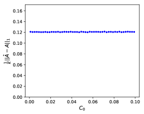
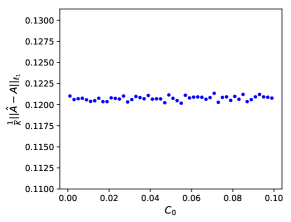
Figure 1: Plots of overall estimation error vs $C_{0}$. The right plot is zoomed in.

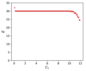
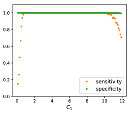
Figure 2: Plots of $\widehat{K}$, sensitivity and specificity vs $C_{1}$ when the true $K_{0}=30$.

Throughout, we consider two versions of our algorithm: Top1 and Top10 described in Algorithm 3 with $T=1$ and $T=10$, respectively. We compare Top with best performing algorithm available, that of Arora et al. (2013). We denote this algorithm by Recover-L2 and Recover-KL depending on which loss function is used for estimating non-anchor rows in their Algorithm 3. In Appendix G we conducted a small simulation study to compare these two methods, and ours, with the recent procedure of Ke and Wang (2017), using the implementation the authors kindly made available to us. Their method is tailored to topic models with a known, small, number of topics. Our study revealed that, in the “small $K$” regime, their procedure is comparable or outperformed by existing methods. Latent Dirichlet Allocation (LDA) (Blei et al., 2003) is a popular Bayesian approach to topic models, but is computationally demanding.

The procedures from Arora et al. (2013) have better performance than LDA in terms of overall loss and computational cost, as evidenced by their simulations. For this reason, we only focus on the comparison of our method with Recover-L2 and Recover-KL for the synthetic data. The comparison with LDA is considered in the semi-synthetic data.

We report the findings of our simulation studies in this section by showing that our algorithms estimate both the number of topics and anchor words consistently, and have superior performance in terms of estimation error as well as computational time in various settings over the existing algorithms.

We re-emphasize that in all the comparisons presented below, the existing methods have as input the true $K$ used to simulate the data, while we also estimate $K$. In Appendix G, we show that these algorithms are very sensitive to the choice of $K$. This demonstrates that correct estimation of $K$ is indeed highly critical for the estimation of the entire matrix $A$.

Topics and anchor words recovery

Top10 and Top1 use the same procedure (Algorithm 2) to select the anchor words, likewise for Recover-L2 and Recover-KL. We present in Table 1 the observed sensitivity ${|\widehat{I}\cap I|/|I|}$ and specificity ${|\widehat{I}^{c}\cap I^{c}|/|I^{c}|}$ of selected anchor words in the benchmark setting with $|I_{k}|$ varying. It is clear that Top recovers all anchor words and estimates the topics number $K$ consistently. All algorithms are performing perfectly for not selecting non-anchor words. We emphasize that the correct $K$ is given for procedure Recover.

Table 1: Table of anchor recovery and topic recovery for varying $|I_{k}|$.

Measures	Top					Recover
$|I_{k}|$	2	4	6	8	10	2	4	6	8	10
sensitivity	$100\%$	$100\%$	$100\%$	$100\%$	$100\%$	$50\%$	$25\%$	$16.7\%$	$12.5\%$	$10\%$
specificity	$100\%$	$100\%$	$100\%$	$100\%$	$100\%$	$100\%$	$100\%$	$100\%$	$100\%$	$100\%$
Number of topics	$100\%$					N/A

Estimation error

In the benchmark setting, we varied $N$ and $n$ over $\{500,1000,1500,2000,2500\}$, $p$ over $\{500,800,1000,1200,1500\}$, $K$ over $\{20,25,30,35,40\}$ and $|I_{k}|$ over $\{2,4,6,8,10\}$, one at a time. For each case, the averaged overall estimation error $\|\widehat{A}-AP\|_{1}/K$ and topic-wise estimation error $\|\widehat{A}-AP\|_{1,\infty}$ over $50$ generated datasets for each dimensional setting were recorded. We used a simple linear program to find the best permutation matrix $P$ which aligns $\widehat{A}$ with $A$. Since the two measures had similar patterns for all settings, we only present overall estimation error in Figure 3, which can be summarized as follows:

• The estimation error of all four algorithms decreases as $n$ or $N$ increases, while it increases as $p$ or $K$ increases. This confirms our theoretical findings and indicates that $A$ is harder to estimate when not only $p$, but $K$ as well, is allowed to grow.

• In all settings, Top10 has the smallest estimation error. Meanwhile, Top1 has better performance than Recover-L2 and Recover-KL except for $N=500$ and $|I_{k}|=2$. The difference between Top10 and Top1 decreases as the length $N$ of each sampled document increases. This is to be expected since the larger the $N$, the better each column of $X$ approximates the corresponding column of $\Pi$, which lessens the benefit of selecting different representative sets $\widehat{L}$ of anchor words.

• Recover-KL is more sensitive to the specification of $K$ and $|I_{k}|$ than the other approaches. Its performance increasingly worsens compared to the other procedures for increasing values of $K$. On the other hand, when the sizes $|I_{k}|$ are small, it performs almost as well as Top10. However, its performance does not improve as much as the performances of the other algorithms in the presence of more anchor words.

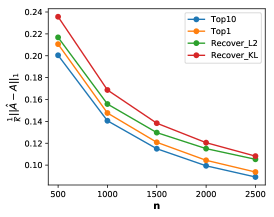
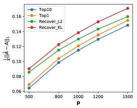
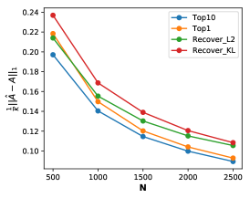
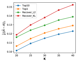
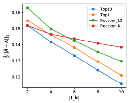
Figure 3: Plots of averaged overall estimation error for varying parameter one at a time.

Running time

The running time of all four algorithms is shown in Figure 4. As expected, Top1 dominates in terms of computational efficiency. Its computational cost only slightly increases in $p$ or $K$. Meanwhile, the running times of Top10 is better than Recover-L2 in most of the settings and becomes comparable to it when $K$ is large or $p$ is small. Recover-KL is overall much more computationally demanding than the others. We see that Top1 and Top10 are nearly independent of $n$, the number of documents, and $N$, the document length, as these parameters only appear in the computations of the matrix $\widehat{R}$ and the tuning parameters $\widehat{\delta}_{ij}$ and $\widehat{\eta}_{ij}$. More importantly, as the dictionary size $p$ increases, the two Recover algorithms become much more computationally expensive than Top. This difference stems from the fact that our procedure of estimating $A$ is almost independent of $p$ computationally. Top solves $K$ linear programs in $K$ dimensional space, while Recover must solve $p$ convex optimization problems over in $K$ dimensional spaces.

We emphasize again that our Top procedure accurately estimates $K$ in the reported times, whereas we provide the two Recover versions with the true values of $K$. In practice, one needs to resort to various cross-validation schemes to select a value of $K$ for the Recover algorithms, see Arora et al. (2013). This would dramatically increase the actual running time for these procedures.

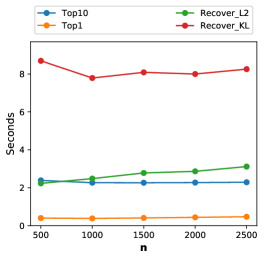
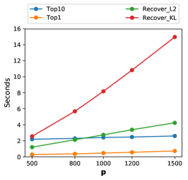
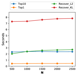
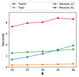
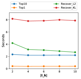
Figure 4: Plots of running time for varying parameter one at a time.

Semi-synthetic data from NIPs corpus

In this section, we compare our algorithm with existing competitors on semi-synthetic data, generated as follows.

We begin with one real-world dataset, a corpus of NIPs articles (Dheeru and Karra Taniskidou, 2017) to benchmark our algorithm and compare Top1 with LDA (Blei et al., 2003), Recover-L2 and Recover-KL. We use the code of LDA from Riddell et al. (2016) implemented via the fast collapsed Gibbs sampling with the default 1000 iterations. To preprocess the data, following Arora et al. (2013), we removed common stopping words and rare words occurring in less than 150 documents, and cut off the documents with less than $150$ words. The resultant dataset has $n=1480$ documents with dictionary size $p=1253$ and mean document length $858$.

To generate semi-synthetic data, we first apply Top to this real data set, in order to obtain the estimated word-topic matrix $A$, which we then use as the ground truth in our simulation experiments, performed as follows. For each document $i\in[n]$, we sample $W_{i}$ from a specific distribution (see below) and we sample $X_{i}$ from $\text{Multinomial}_{p}(N_{i},AW_{i})$. The estimated $A$ from Top (with $C_{1}=4.5$ chosen via cross-validation and $C_{0}=0.01$) contains 178 anchor words and $120$ topics. We consider three distributions of $W$, chosen as in (Arora et al., 2013):

1. symmetric Dirichlet distribution with parameter $0.03$;

2. logistic-normal distribution with block diagonal covariance matrix and $\rho=0.02$;

3. logistic-normal distribution with block diagonal covariance matrix and $\rho=0.2$.

Cases (b) and (c) are designed to investigate how the correlation among topics affects the estimation error. To construct the block diagonal covariance structure, we divide the 120 topics into 10 groups. For each group, the off-diagonal elements of the covariance matrix of topics is set to $\rho$ while the diagonal entries are set to $1$. The parameter $\rho=\{0.02,0.2\}$ reflects the magnitude of correlation among topics.

The number of documents $n$ is varied as $\{2000,3000,4000,5000,6000\}$ and the document length is set to $N_{i}=850$ for $1\leq i\leq n$. In each setting, we repeat generating 20 datasets and report the averaged overall estimation error $\|\widehat{A}-AP\|_{1}/K$ and topic-wise estimation error $\|\widehat{A}-AP\|_{1,\infty}$ of different algorithms in Figure 5. The running time of each algorithm is reported in Table 2.

Overall, LDA is outperformed by the other three methods, though its performance might be improved by increasing the number of iterations. Top, Recover-KL and Recover-L2 are comparable when columns of $W$ are sampled from a symmetric Dirichlet with parameter 0.03, whereas Top has better performance when the correlation among topics increases. Moreover, Top has the best control of topic-wise estimation error as expected, while the comparison between Recover-KL and Recover-L2 depends on the error metric. From the running-time perspective, Top runs significantly faster than the other three methods.

Finally, we emphasize that we provide LDA and the two Recover algorithms with the true $K$, whereas Top estimates it.

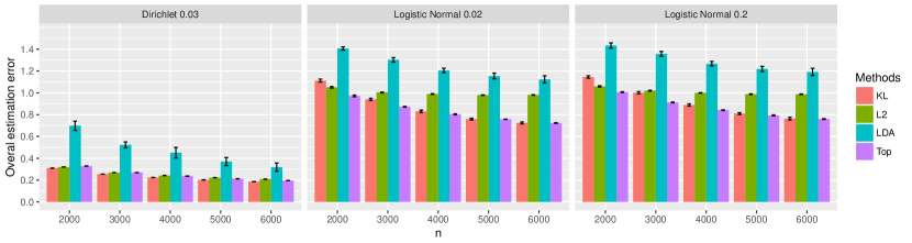
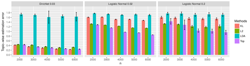
Figure 5: Plots of averaged overall estimation error and topic-wise estimation error of Top, Recover-L2 (L2), Recover-KL (KL) and LDA. TOP estimates $K$, the other methods use the true $K$ as input. The bars denote one standard deviation.

Table 2: Running time (seconds) of different algorithms

	Top	Recover-L2	Recover-KL	LDA
$n=2000$	21.4	428.2	2404.5	3052.3
$n=3000$	22.3	348.2	1561.8	4649.5
$n=4000$	25.3	353.5	1764.8	6051.1
$n=5000$	28.5	349.0	1800.4	7113.0
$n=6000$	29.5	346.6	1848.1	7318.4

Supplement

From the topic model specifications, the matrices $\Pi$, $A$ and $W$ are all scaled as

$$\sum_{j=1}^{p}\Pi_{ji}=1,\quad\sum_{j=1}^{p}A_{jk}=1,\quad\sum_{k=1}^{K}W_{ki}=1$$ (52)

for any $1\leq j\leq p$, $1\leq i\leq n$ and $1\leq k\leq K$. In order to adjust their scales properly, we denote

$$m_{j}=p\max_{1\leq i\leq n}\Pi_{ji},~{}~{}\mu_{j}={p\over n}\sum_{i=1}^{n}\Pi_{ji},~{}~{}\alpha_{j}=p\max_{1\leq k\leq K}A_{jk},~{}~{}\gamma_{k}={K\over n}\sum_{i=1}^{n}W_{ki},$$ (53)

so that

$$\sum_{k=1}^{K}\gamma_{k}=K,\qquad\sum_{j=1}^{p}\mu_{j}=p.$$ (54)

We further denote $m_{\min}=\min_{1\leq j\leq p}m_{j}$ and $\mu_{\min}=\min_{1\leq j\leq p}\mu_{j}.$

Appendix A Proofs of Section 2

Proof of Proposition 1.

Recall that $Y_{i}:=N_{i}X_{i}\sim\text{Multinomial}_{p}(N_{i};\Pi_{i})$ for any $i\in[n]$. The joint log-likelihood of $(Y_{1},\ldots,Y_{n})$ is

$$\ell(Y_{1},\ldots,Y_{n}) =\sum_{i=1}^{n}\log(N_{i}!)-\sum_{i=1}^{n}\sum_{j=1}^{p}\log(Y_{ji})+\sum_{i=1}^{n}\sum_{j=1}^{p}Y_{ji}\log\Pi_{ji}$$

$$=\sum_{i=1}^{n}\log(N_{i}!)-\sum_{i=1}^{n}\sum_{j=1}^{p}\log(Y_{ji})+\sum_{i=1}^{n}\sum_{j=1}^{p}Y_{ji}\log\left(\sum_{k=1}^{K}A_{jk}W_{ki}\right).$$

Fix any $j\in[p]$, $k\in[K]$ and $i\in[n]$. It follows that

$${\partial\ell(Y_{1},\ldots,Y_{n})\over\partial A_{jk}}=\left\{\begin{array}[]{ll}\sum_{i=1}^{n}Y_{ji}W_{ki}\Big{/}\left(\sum_{t=1}^{K}A_{jt}W_{ti}\right),&\text{if }A_{jk}\neq 0,W_{ki}\neq 0\\ 0,&\text{otherwise}\end{array}\right.$$

from which we further deduce

$${\partial^{2}\ell(Y_{1},\ldots,Y_{n})\over\partial A_{jk}\partial W_{ki}}$$

$$=\left\{\begin{array}[]{ll}\sum_{i=1}^{n}Y_{ji}\left(\sum_{t=1}^{K}A_{jt}W_{ti}-A_{jk}W_{ki}\right)\Big{/}\left(\sum_{t=1}^{K}A_{jt}W_{ti}\right)^{2},&\text{if }A_{jk}\neq 0,W_{ki}\neq 0\\ 0,&\text{otherwise}\end{array}\right..$$

Since $\mathbb{E}[Y_{ji}]=N_{i}\Pi_{ji}$, taking expectation yields

$$\mathbb{E}\left[-{\partial^{2}\ell(Y_{1},\ldots,Y_{n})\over\partial A_{jk}\partial W_{ki}}\right]$$

$$=\left\{\begin{array}[]{ll}\sum_{i=1}^{n}N_{i}\left(\sum_{t\neq k}A_{jt}W_{ti}\right)\Big{/}\left(\sum_{t=1}^{K}A_{jt}W_{ti}\right),&\text{if }A_{jk}\neq 0,W_{ki}\neq 0\\ 0,&\text{otherwise}\end{array}\right..$$ (57)

Similarly, for this $j$, $k$ and $i$ but with any $k^{\prime}\neq k$, we have

$${\partial^{2}\ell(Y_{1},\ldots,Y_{n})\over\partial A_{jk}\partial W_{k^{\prime}i}}$$

$$=\left\{\begin{array}[]{ll}-\sum_{i=1}^{n}Y_{ji}A_{jk^{\prime}}W_{ki}\Big{/}\left(\sum_{t=1}^{K}A_{jt}W_{ti}\right)^{2},&\text{if }A_{jk}\neq 0,A_{jk^{\prime}}\neq 0,W_{k^{\prime}i}\neq 0,W_{ki}\neq 0\\ 0,&\text{otherwise}\end{array}\right.$$

and

$$\mathbb{E}\left[-{\partial^{2}\ell(Y_{1},\ldots,Y_{n})\over\partial A_{jk}\partial W_{k^{\prime}i}}\right]$$

$$=\left\{\begin{array}[]{ll}\sum_{i=1}^{n}N_{i}A_{jk^{\prime}}W_{ki}\Big{/}\sum_{t=1}^{K}A_{jt}W_{ti},&\text{if }A_{jk}\neq 0,A_{jk^{\prime}}\neq 0,W_{k^{\prime}i}\neq 0,W_{ki}\neq 0\\ 0,&\text{otherwise}\end{array}\right..$$ (60)

From (A) and (A), it is easy to see that condition (7) implies

$$\mathbb{E}\left[-{\partial^{2}\ell(Y_{1},\ldots,Y_{n})\over\partial A_{jk}\partial W_{k^{\prime}i}}\right]=0$$ (61)

for any $j\in[p]$, $k,k^{\prime}\in[K]$ and $i\in[n]$. This proves the sufficiency. To show the necessity, we use contradiction. If (61) holds for any $j\in[p]$, $k,k^{\prime}\in[K]$ and $i\in[n]$, suppose there exist at least one $j\in[p]$ and $i\in[n]$ such that $\textrm{supp}(A_{j\cdot})\cap\textrm{supp}(W_{\cdot i})=\{k_{1},k_{2}\}$ and $k_{1}\neq k_{2}$. Then, (A) implies

$$\mathbb{E}\left[-{\partial^{2}\ell(Y_{1},\ldots,Y_{n})\over\partial A_{jk_{1}}\partial W_{k_{2}i}}\right]\geq{N_{i}A_{jk_{1}}W_{k_{2}i}\over A_{jk_{1}}W_{k_{1}i}+A_{jk_{2}}W_{k_{2}i}}\neq 0.$$

This contradicts (7) and concludes the proof. ∎

Proof of Proposition 2.

Since the columns of $A$ sum up to 1, and Assumption 1 holds, then the matrix $\widetilde{A}$ satisfies:

$$\widetilde{A}_{jk}\geq 0,\quad\bigl{\|}\widetilde{A}_{j\cdot}\bigr{\|}_{1}=1,\qquad\text{ for each }j=1,\ldots,p,\text{ and }K=1,\ldots,K.$$ (62)

Additionally, $\widetilde{A}$ has the same sparsity pattern as $A$, and thus $\widetilde{A}$ satisfies Assumption 1, with the same $I$ and $\mathcal{I}$. We further notice that Assumption 3 is equivalent to

$$|\langle\widetilde{W}_{i\cdot},\widetilde{W}_{j\cdot}\rangle|~{}<~{}\|\widetilde{W}_{i\cdot}\|^{2}\wedge\|\widetilde{W}_{j\cdot}\|^{2},\qquad\text{for all $1\leq i<j\leq K$,}$$

which is further equivalent with $\nu>0$, defined in (23).

To finish the proof we invoke Theorem 1 in Bing et al. (2017), slightly adapted to our situation. Specifically, we consider any matrix $R$ defined in (11) that factorizes as $R=\widetilde{A}\widetilde{C}\widetilde{A}^{T}$ where $\widetilde{A}$ satisfies Assumption 1 and $\widetilde{C}$ satisfies (23). Note that the quantities $M_{i}$ and $S_{i}$ defined in page 9 of Bing et al. (2017) are replaced by, respectively, $T_{i}$ and $S_{i}$ in (12). We proceed to prove $(a)$ and $(b)$ of Proposition 2.

Proof of $(a)$. We first show the sufficiency part. Consider any $i\in[p]$ with $T_{i}=T_{j}$ for all $j\in S_{i}$. Part (a) of Lemma 10, stated after the proof, states that there exists a $j\in I_{a}\cap S_{i}$ for some $a\in[K]$. For this $j\in I_{a}$, we have $T_{j}=\widetilde{C}_{aa}$ from part (b) of Lemma 10. Invoking our premise $T_{j}=T_{i}$ as $j\in S_{i}$, we conclude that $T_{i}=\widetilde{C}_{aa}$, that is, $\max_{k\in p}R_{ik}=\widetilde{C}_{aa}$. By Lemma 9, stated after the proof, the maximum is achieved for any $i\in I_{a}$. However, if $i\not\in I_{a}$, we have that $R_{ik}<\widetilde{C}_{aa}$ for all $k\in[p]$. Hence $i\in I_{a}$ and this concludes the proof of the sufficiency part.

It remains to prove the necessity part. Let $i\in I_{a}$ for some $a\in[K]$ and $j\in S_{i}$. Lemma 10 implies that $j\in I_{a}$ and $T_{i}=C_{aa}$. Since $j\in S_{i}$, we have $R_{ij}=T_{i}=\widetilde{C}_{aa}$, while $j\in I_{a}$ yields $R_{jk}\leq\widetilde{C}_{aa}$ for all $k\in[p]$, and $R_{j}k=\widetilde{C}_{aa}$ for $k\in I_{a}$, as a result of Lemma 9. Hence, $T_{j}=\max_{k\in[p]}R_{jk}=\widetilde{C}_{aa}=T_{i}$ for any $j\in S_{i}$, which proves our claim.

Proof of $(b)$. The proof of $(b)$ follows by the same arguments for proving part ${\bf(b)}$ of Theorem 1 in Bing et al. (2017). The proof is then complete. ∎

The following two lemmas are used in the above proof. They are adapted from Lemmas 1 and 2 of the supplement of Bing et al. (2017).

Lemma 9.

For any $a\in[K]$ and $i\in I_{a}$, we have

• $R_{ij}=\widetilde{C}_{aa}$ for all $j\in I_{a}$,

• $R_{ij}<\widetilde{C}_{aa}$ for all $j\not\in I_{a}$.

Proof.

The proof follows the same argument for proving Lemma 1 in Bing et al. (2017). ∎

Lemma 10.

Let $T_{i}$ and $S_{i}$ be defined in (12). We have

• $S_{i}\cap I\neq\varnothing$, for any $i\in[p]$,

• $S_{i}\cup\{i\}=I_{a}$ and $T_{i}=\widetilde{C}_{aa}$, for any $i\in I_{a}$ and $a\in[K]$.

Proof.

Lemma 9 implies that, for any $i\in I_{a}$, $T_{i}=\widetilde{C}_{aa}$ and $S_{i}=I_{a}$, which proves part (b). Part (a) follows from the result of part (b) and the same arguments of the proof of Lemma 2 in Bing et al. (2017) by replacing $M_{i}$ by $T_{i}$, $|\Sigma_{ij}|$ by $R_{ij}$, $A$ by $\widetilde{A}$ and $C$ by $\widetilde{C}$. ∎

Appendix B Error bounds of stochastic errors

We use this section to present tight bounds on the error terms which are critical to our later estimation rate. We recall that $\varepsilon_{ji}:=X_{ji}-\Pi_{ji}$, for $1\leq i\leq n$ and $1\leq j\leq p$ and assume $N_{1}=\ldots=N_{n}=N$ for ease of presentation since similar results for different $N$ can be derived by using the same arguments. The following results, Lemmata 13 - 15 control several terms related with $\varepsilon_{ji}$ under the multinomial assumption (2). We start by stating the well-known Bernstein inequality and Hoeffding inequality for bounded random variables which are used in the sequel.

Lemma 11 (Bernstein’s inequality for bounded random variable).

For independent random variables $Y_{1},\ldots,Y_{n}$ with bounded ranges $[-B,B]$ and zero means,

$$\mathbb{P}\left\{{1\over n}\left|\sum_{i=1}^{n}Y_{i}\right|>x\right\}\leq 2\exp\left(-{n^{2}x^{2}/2\over v+nBx/3}\right),\qquad\text{for any }x\geq 0,$$

where $v\geq var(Y_{1}+\ldots+Y_{n})$.

Lemma 12 (Hoeffding’s inequality).

Let $Y_{1},\ldots,Y_{n}$ be independent random variables with $\mathbb{E}[Y_{i}]=0$ and bounded by $[a_{i},b_{i}]$: For any $t\geq 0$, we have

$$\mathbb{P}\left\{\left|\sum_{i=1}^{n}Y_{i}\right|>t\right\}\leq 2\exp\left(-\frac{2t^{2}}{\sum_{i=1}^{n}(b_{i}-a_{i})^{2}}\right).$$

Lemma 13.

Assume $\mu_{\min}/p\geq 2\log M/(3N)$. With probability $1-2M^{-1}$,

$${1\over n}\left|\sum_{i=1}^{n}\varepsilon_{ji}\right|\leq 2\sqrt{\mu_{j}\log M\over npN}\left(1+\sqrt{6}n^{-{1\over 2}}\right),\quad\text{uniformly in $1\leq j\leq p$.}$$

Proof.

Fix $1\leq j\leq p$. From model (3), we know $NX_{ji}\sim$ Binomial$(N;\Pi_{ji})$. We express the binomial random variable as a sum of i.i.d. Bernoulli random variables:

$$\varepsilon_{ji}=X_{ji}-\Pi_{ji}={1\over N}\sum_{k=1}^{N}\left(B_{ik}^{j}-\Pi_{ji}\right):={1\over N}\sum_{\ell=1}^{N}Z^{j}_{ik}$$

with $B_{i\ell}^{j}\sim$ Bernoulli$(\Pi_{ji})$, such that $N\sum_{i=1}^{n}\varepsilon_{ji}=\sum_{i=1}^{n}\sum_{\ell=1}^{N}Z^{j}_{i\ell}.$ Note that $|Z_{ik}^{j}|\leq 1$, $\mathbb{E}[Z_{ik}^{j}]=0$ and $\mathbb{E}[(Z^{j}_{ik})^{2}]=\Pi_{ji}(1-\Pi_{ji})\leq\Pi_{ji}$, for all $i\in[n]$ and $k\in[N]$. An application of Bernstein’s inequality, see Lemma 11, to $Z_{i\ell}^{j}$ with $v=N\sum_{i=1}^{n}\Pi_{ji}=Nn\mu_{j}/p$ and $B=1$ gives

$$\mathbb{P}\left\{{1\over n}\left|\sum_{i=1}^{n}\varepsilon_{ji}\right|>t\right\}\leq 2\exp\left(-{n^{2}N^{2}t^{2}/2\over N\sum_{i=1}^{n}\Pi_{ji}+nNt/3}\right),\quad\text{for any $t>0$.}$$

This implies, for all $t>0$

$$\mathbb{P}\left\{{1\over n}\left|\sum_{i=1}^{n}\varepsilon_{ji}\right|>{\sqrt{\mu_{j}t\over npN}}+{t\over nN}\right\}\leq 2e^{-t/2}.$$

Choosing $t=4\log M$ and recalling that $M=n\vee N\vee p\geq p$, we find by the union bound

$$\sum_{j=1}^{p}\mathbb{P}\left\{{1\over n}\left|\sum_{i=1}^{n}\varepsilon_{ji}\right|>2{\sqrt{\mu_{j}\log M\over npN}}+{4\log M\over nN}\right\}\leq 2pM^{-2}\leq 2M^{-1}.$$ (63)

Using $\mu_{\min}/p\geq 2\log M/(3N)$ concludes the proof. ∎

Remark 13.

By inspection of the proof of Lemma 13, if instead of the bound $\mathbb{E}[(Z_{ik}^{j})^{2}]\leq\Pi_{ji}$, we had used the overall bound $\mathbb{E}[(Z_{ik}^{j})^{2}]\leq 1$, and application of Bernstein’s inequality would yield,

$${1\over n}\left|\sum_{i=1}^{n}\varepsilon_{ji}\right|\leq c{\sqrt{\log M\over nN}},\quad\text{uniformly in $1\leq j\leq p$.}$$

Summing over $1\leq j\leq p$ in the above display would further give

$${1\over n}\sum_{j=1}^{p}\left|\sum_{i=1}^{n}\varepsilon_{ji}\right|\leq c\cdot p{\sqrt{\log M\over nN}},$$

and the right hand side would be slower by an important $\sqrt{p}$ factor that what we would obtain by summing the bound in Lemma 13 over $1\leq j\leq p$, since

$$2\sum_{j=1}^{p}\sqrt{\mu_{j}\log M\over npN}\leq 2\sqrt{\log M\over nN}\sqrt{\sum_{j=1}^{p}\mu_{j}}=2\sqrt{p\log M\over nN}.$$

In this last display, we used the Cauchy-Schwarz inequality in the first inequality, and the constraint (54) in the last equality. The bound of Lemma 13 is an important intermediate step for deriving the final bounds of Theorem 7, and the simple calculations presented above that the constraints of unit column sums induced by model (3) permit a more refined control of the stochastic errors than those previously considered. A larger impact of this refinement on the final rate of convergence is illustrated in Remark 14, following the proof of Lemma 15, in which we control sums of quadratic, dependent terms $\varepsilon_{ji}\varepsilon_{\ell i}$.

Lemma 14.

With probability $1-2M^{-1}$,

$${1\over n}\left|\sum_{i=1}^{n}\Pi_{\ell i}\varepsilon_{ji}\right|\leq{\sqrt{6m_{\ell}\Theta_{j\ell}\log M\over npN}}+{2m_{\ell}\log M\over npN},\quad\text{uniformly in $1\leq j,\ell\leq p$.}$$

Proof.

Similar as in the proof of Lemma 13, we write

$$\Pi_{\ell i}\varepsilon_{ji}={1\over N}\sum_{k=1}^{N}\Pi_{\ell i}Z_{ik}^{j}$$

such that $|\Pi_{\ell i}Z_{ik}^{j}|\leq\Pi_{\ell i}\leq m_{\ell}/p$ by (53), $\mathbb{E}[\Pi_{\ell i}Z_{ik}^{j}]=0$ and $\mathbb{E}[\Pi_{\ell i}^{2}Z_{ik}^{2}]=\Pi_{\ell i}^{2}\Pi_{ji}(1-\Pi_{ji})\leq m_{\ell}\Pi_{\ell i}\Pi_{ji}/p$, for all $i\in[n]$ and $k\in[N]$. Fix $1\leq j,\ell\leq p$ and recall that $\Theta_{j\ell}=n^{-1}\sum_{i=1}^{n}\Pi_{ji}\Pi_{\ell i}$. Applying Bernstein’s inequality to $\Pi_{\ell i}Z_{ik}^{j}$ with $v=nNm_{\ell}\Theta_{j\ell}/p$ and $B=m_{\ell}/p$ gives

$$\mathbb{P}\left\{{1\over n}\left|\sum_{i=1}^{n}\Pi_{\ell i}\varepsilon_{ji}\right|\geq t\right\}\leq 2\exp\left(-{n^{2}N^{2}t^{2}/2\over nNm_{\ell}\Theta_{j\ell}/p+nNm_{\ell}t/(3p)}\right)$$

which further implies

$$\mathbb{P}\left\{{1\over n}\left|\sum_{i=1}^{n}\Pi_{\ell i}\varepsilon_{ji}\right|>\sqrt{m_{\ell}\Theta_{j\ell}t\over npN}+{m_{\ell}t\over 3npN}\right\}\leq 2e^{-t/2}.$$

Taking the union bound over $1\leq j,\ell\leq p$, and choosing $t=6\log M$, concludes the proof. ∎

Lemma 15.

If $\mu_{\min}/p\geq 2\log M/(3N)$, then with probability $1-4M^{-1}$,

$${1\over n}\left|\sum_{i=1}^{n}\left(\varepsilon_{ji}\varepsilon_{\ell i}-\mathbb{E}[\varepsilon_{ji}\varepsilon_{\ell i}]\right)\right|\leq 12\sqrt{6}\sqrt{\Theta_{j\ell}+{(\mu_{j}+\mu_{\ell})\log M\over pN}}\sqrt{(\log M)^{3}\over nN^{2}}+4M^{-3},$$

holds, uniformly in $1\leq j,\ell\leq p$.

Proof.

For any $1\leq j\leq p$, recall that $\varepsilon_{ji}=X_{ji}-\Pi_{ji}$ and

$$\varepsilon_{ji}={1\over N}\sum_{k=1}^{N}Z_{ik}^{j}$$

where $Z_{ik}^{j}:=B_{ik}^{j}-\Pi_{ji}$ and $B_{ik}^{j}\sim$ Bernoulli$(\Pi_{ji})$. By using the arguments of Lemma 13, application of Bernstein’s inequality to $Z_{ik}^{j}$ with $v=N\Pi_{ji}$ and $B=1$ gives

$$\mathbb{P}\left\{\left|\varepsilon_{ji}\right|>t\right\}\leq 2\exp\left(-{Nt^{2}/2\over\Pi_{ji}+t/3}\right),\quad\text{ for any $t>0$,}$$

which yields

$$\left|\varepsilon_{ji}\right|\leq{\sqrt{6\Pi_{ji}\log M\over N}}+{2\log M\over N}:=T_{ji}$$

with probability greater than $1-2M^{-3}$. We define $Y_{ji}=\varepsilon_{ji}\mathbbm{1}_{\mathcal{S}_{ji}}$ with $\mathcal{S}_{ji}:=\left\{|\varepsilon_{ji}|\leq T_{ji}\right\}$ for each $1\leq j\leq p$ and $1\leq i\leq n$, and $\mathcal{S}:=\cap_{j=1}^{p}\cap_{i=1}^{n}\mathcal{S}_{ji}.$ It follows that $\mathbb{P}(\mathcal{S}_{ji})\geq 1-2M^{-3}$ for all $1\leq i\leq n$ and $1\leq j\leq p$, so that $\mathbb{P}(\mathcal{S})\geq 1-2M^{-1}$ as $M:=n\vee p\vee N$. On the event $\mathcal{S}$, we have

$${1\over n}\left|\sum_{i=1}^{n}\left(\varepsilon_{ji}\varepsilon_{\ell i}-\mathbb{E}[\varepsilon_{ji}\varepsilon_{\ell i}]\right)\right|\leq\underbrace{{1\over n}\left|\sum_{i=1}^{n}\left(Y_{ji}Y_{\ell i}-\mathbb{E}[Y_{ji}Y_{\ell i}]\right)\right|}_{T_{1}}+\underbrace{{1\over n}\left|\sum_{i=1}^{n}\left(\mathbb{E}[\varepsilon_{ji}\varepsilon_{\ell i}]-\mathbb{E}[Y_{ji}Y_{\ell i}]\right)\right|}_{T_{2}}$$

We first study $T_{2}$. By writing

$$\mathbb{E}[\varepsilon_{ji}\varepsilon_{\ell i}] =\mathbb{E}[Y_{ji}Y_{\ell i}]+\mathbb{E}\left[Y_{ji}\varepsilon_{\ell i}\mathbbm{1}_{\mathcal{S}_{\ell i}^{c}}\right]+\mathbb{E}\left[\varepsilon_{ji}\mathbbm{1}_{\mathcal{S}_{ji}^{c}}\varepsilon_{\ell i}\right],$$

we have

$$T_{2}={1\over n}\left|\sum_{i=1}^{n}\left(\mathbb{E}[\varepsilon_{ji}\varepsilon_{\ell i}]-\mathbb{E}[Y_{ji}Y_{\ell i}]\right)\right| \leq{1\over n}\left|\sum_{i=1}^{n}\left(\mathbb{E}\left[Y_{ji}\varepsilon_{\ell i}\mathbbm{1}_{\mathcal{S}_{\ell i}^{c}}\right]+\mathbb{E}\left[\varepsilon_{ji}\mathbbm{1}_{\mathcal{S}_{ji}^{c}}\varepsilon_{\ell i}\right]\right)\right|$$

$$\leq{1\over n}\left|\sum_{i=1}^{n}\left(\mathbb{P}(\mathcal{S}_{ji}^{c})+\mathbb{P}(\mathcal{S}_{\ell i}^{c})\right)\right|$$ (64)

$$\leq 4M^{-3}$$

by using $|Y_{ji}|\leq|\varepsilon_{ji}|\leq 1$ in the second inequality.

Next we bound $T_{1}$. Since $|Y_{ji}|\leq T_{ji}$, we know $-2T_{ji}T_{\ell i}\leq Y_{ji}Y_{\ell i}-\mathbb{E}[Y_{ji}Y_{\ell i}]\leq 2T_{ji}T_{\ell i}$ for all $1\leq i\leq n$. Applying the Hoeffding inequality Lemma 12 with $a_{i}=-2T_{ji}T_{\ell i}$ and $b_{i}=2T_{ji}T_{\ell i}$ gives

$$\mathbb{P}\left\{\left|\sum_{i=1}^{n}\left(Y_{ji}Y_{\ell i}-\mathbb{E}[Y_{ji}Y_{\ell i}]\right)\right|\geq t\right\}\leq 2\exp\left(-{t^{2}\over 8\sum_{i=1}^{n}T_{ji}^{2}T_{\ell i}^{2}}\right).$$

Taking $t=\sqrt{24\sum_{i=1}^{n}T_{ji}^{2}T_{\ell i}^{2}\log M}$ yields

$$T_{1}={1\over n}\left|\sum_{i=1}^{n}\left(Y_{ji}Y_{\ell i}-\mathbb{E}[Y_{ji}Y_{\ell i}]\right)\right|\leq 2\sqrt{6}\left({1\over n}\sum_{i=1}^{n}T_{ji}^{2}T_{\ell i}^{2}\cdot{\log M\over n}\right)^{1/2}$$ (65)

with probability greater than $1-2M^{-3}$. Finally, note that

$${1\over n}\sum_{i=1}^{n}T_{ji}^{2}T_{\ell i}^{2} ={1\over n}\sum_{i=1}^{n}\left(\Pi_{ji}\Pi_{\ell i}{36(\log M)^{2}\over N^{2}}+\left(2\log M\over N\right)^{4}+(\Pi_{ji}+\Pi_{\ell i}){24(\log M)^{3}\over N^{3}}\right)$$

$$=36\Theta_{j\ell}\left(\log M\over N\right)^{2}+16\left({\log M\over N}\right)^{4}+24(\mu_{j}+\mu_{\ell}){(\log M)^{3}\over pN^{3}}$$ (66)

by using (53) and $\Theta_{j\ell}=n^{-1}\Pi\Pi^{T}$ in the second equality. Finally, combining (64) - (B) and using $\mu_{\min}/p\geq 2\log M/(3N)$ conclude the proof. ∎

Remark 14.

We illustrate the improvement of our result over a simple application of Hanson-Wright inequality. Write

$$4\varepsilon_{ji}\varepsilon_{\ell i}=\left(\varepsilon_{ji}+\varepsilon_{\ell i}\right)^{2}-\left(\varepsilon_{ji}-\varepsilon_{\ell i}\right)^{2}$$

for each $i\in[n]$. Since $\varepsilon_{ji}=N^{-1}\sum_{k=1}^{N}Z_{ik}^{j}$ and $\|\varepsilon_{ji}\pm\varepsilon_{\ell i}\|_{\phi_{2}}\leq{2/\sqrt{N}}$, a direct application of the Hanson-Wright inequality to the two terms in the right hand side will give

$${1\over n}\left|\sum_{i=1}^{n}\left(\varepsilon_{ji}\varepsilon_{\ell i}-\mathbb{E}[\varepsilon_{ji}\varepsilon_{\ell i}]\right)\right|\leq c\sqrt{\log M\over nN}$$

with high probability. Summing over $1\leq j\leq p$ and $1\leq\ell\leq p$ further yields

$$\sum_{j,\ell=1}^{p}{1\over n}\left|\sum_{i=1}^{n}\left(\varepsilon_{ji}\varepsilon_{\ell i}-\mathbb{E}[\varepsilon_{ji}\varepsilon_{\ell i}]\right)\right|\leq c\cdot p^{2}\sqrt{\log M\over nN}.$$ (67)

By contrast, summing the first term in Lemma 15 yields

$$\sum_{j,\ell=1}^{p}{1\over n}\left|\sum_{i=1}^{n}\left(\varepsilon_{ji}\varepsilon_{\ell i}-\mathbb{E}[\varepsilon_{ji}\varepsilon_{\ell i}]\right)\right| \leq c\cdot\sqrt{p^{2}(\log M)^{3}\over nN^{2}}\sqrt{\sum_{1\leq j,\ell\leq p}\Theta_{j\ell}}+c\cdot\sqrt{p^{3}(\log M)^{4}\over nN^{3}}$$

$$=c\cdot\sqrt{p^{2}(\log M)^{3}\over nN^{2}}+c\cdot\sqrt{p^{3}(\log M)^{4}\over nN^{3}}$$

by using Cauchy-Schwarz in the first inequality and (52) in the last equality which is $(p\sqrt{N})\wedge(N\sqrt{p})$ faster than the result in (67) after ignoring the logarithmic term.

Appendix C Proofs of Section 4

Throughout this section, we define the event $\mathcal{E}:=\mathcal{E}_{1}\cap\mathcal{E}_{2}\cap\mathcal{E}_{3}$ by

$$\mathcal{E}_{1} =\bigcap_{j=1}^{p}\left\{{1\over n}\left|\sum_{i=1}^{n}\varepsilon_{ji}\right|\leq 2(1+\sqrt{6/n})\sqrt{\mu_{j}\log M\over npN}\right\},$$

$$\mathcal{E}_{2} =\bigcap_{j,\ell=1}^{p}\left\{{1\over n}\left|\sum_{i=1}^{n}\Pi_{\ell i}\varepsilon_{ji}\right|\leq{\sqrt{6m_{\ell}\Theta_{j\ell}\log M\over npN}}+{2m_{\ell}\log M\over npN}\right\},$$

$$\mathcal{E}_{3} =\bigcap_{j,\ell=1}^{p}\left\{{1\over n}\left|\sum_{i=1}^{n}\left(\varepsilon_{ji}\varepsilon_{\ell i}-\mathbb{E}[\varepsilon_{ji}\varepsilon_{\ell i}]\right)\right|\leq 12\sqrt{6}\sqrt{\Theta_{j\ell}+{(\mu_{j}+\mu_{\ell})\log M\over pN}}\sqrt{(\log M)^{3}\over nN^{2}}+4M^{-3}\right\}$$

Recall (53) and (54), if

$$\min_{1\leq j\leq p}{1\over n}\sum_{i=1}^{n}\Pi_{ji}\geq{2\log M\over 3N}$$

holds, we have

$${1\over p}\geq{\mu_{\min}\over p}=\min_{1\leq j\leq p}{1\over n}\sum_{i=1}^{n}\Pi_{ji}\geq{2\log M\over 3N},$$ (68)

Therefore, invoking Lemmas 13 – 15 yields $\mathbb{P}(\mathcal{E})\geq 1-8M^{-1}$.

C.1 Preliminaries

From model specifications (52) and (53), we first give some useful expressions which are repeatedly invoked later.

• For any $j\in[p]$, by using (53),

  $$\mu_{j}={p\over n}\sum_{i=1}^{n}\Pi_{ji}={p\over n}\sum_{i=1}^{n}\sum_{k=1}^{K}A_{jk}W_{ki}={p\over K}\sum_{k=1}^{K}A_{jk}\gamma_{k}~{}~{}\Rightarrow~{}~{}{p\over K}\sum_{k=1}^{K}A_{jk}\cdot\underline{\gamma}\leq\mu_{j}\leq\alpha_{j}.$$ (69)

  In particular, for any $j\in I_{k}$ with any $k\in[K]$,

  $$\mu_{j}={p\over n}\sum_{i=1}^{n}\sum_{k=1}^{K}A_{jk}W_{ki}={p\over K}A_{jk}\gamma_{k}\overset{(\ref{def_uag})}{=}{\alpha_{j}\gamma_{k}\over K}.$$ (70)

• For any $j\in[p]$,

  $$m_{j}\overset{(\ref{def_uag})}{=}{p}\max_{1\leq i\leq n}\Pi_{ji}={p}\max_{1\leq i\leq n}\sum_{k=1}^{K}A_{jk}W_{ki}\leq p\max_{1\leq k\leq K}A_{jk}\overset{(\ref{def_uag})}{=}\alpha_{j}~{}~{}\Rightarrow~{}~{}\mu_{j}\leq m_{j}\leq\alpha_{j},$$ (71)

  by using $0\leq W_{ki}\leq 1$ and $\sum_{k}W_{ki}=1$ for any $k\in[K]$ and $i\in[n]$.

C.2 Control of $\widehat{\Theta}-\Theta$ and $\widehat{R}-R$

Proposition 16.

Under model (3), assume (26). Let $\widehat{\Theta}$ and $\widehat{R}$ be defined in (20) and (21), respectively. Then $\widehat{\Theta}$ is an unbiased estimator of $\Theta$. Moreover, with probability greater than $1-8M^{-1}$,

$$|\widehat{\Theta}_{j\ell}-\Theta_{j\ell}|\leq\eta_{j\ell},\qquad|\widehat{R}_{j\ell}-R_{j\ell}|\leq\delta_{j\ell}$$

for all $1\leq j,\ell\leq p$, where

$$\eta_{j\ell} :=3\sqrt{6}\left(\sqrt{m_{j}\over p}+\sqrt{m_{\ell}\over p}\right)\sqrt{\Theta_{j\ell}\log M\over nN}+{2(m_{j}+m_{\ell})\over p}{\log M\over nN}$$

$$\qquad+31(1+\kappa_{1})\sqrt{{\mu_{j}+\mu_{\ell}\over p}{(\log M)^{4}\over nN^{3}}}+\kappa_{2}$$ (72)

and

$$\delta_{j\ell}:=(1+\kappa_{1}\kappa_{3}){p^{2}\over\mu_{j}\mu_{\ell}}\eta_{j\ell}+\kappa_{3}{p^{2}\Theta_{j\ell}\over\mu_{j}\mu_{\ell}}\left(\sqrt{p\over\mu_{j}}+\sqrt{p\over\mu_{\ell}}\right)\sqrt{\log M\over nN},$$ (73)

with $\kappa_{1}=\sqrt{6/n}$, $\kappa_{2}=4/M^{3}$ and

$$\kappa_{3}={2(1+\kappa_{1})\over(1-\kappa_{1}-\kappa_{1}^{2})^{2}}.$$

Remark 15.

For ease of presentation, we assumed that the document lengths are equal, that is, $N_{i}=N$ for all $i\in[n]$. Inspection of the proofs of Lemmas 13 - 15 and Proposition 16, we may allow for unequal document lengths $N_{i}$ by adjusting the quantities $\eta_{j\ell}$ and $\delta_{j\ell}$ with

$$\eta_{j\ell} :=3\sqrt{6}\left(\sqrt{m_{j}}+\sqrt{m_{\ell}}\right)\sqrt{\log M\over np}\left({1\over n}\sum_{i=1}^{n}{\Pi_{ji}\Pi_{\ell i}\over N_{i}}\right)^{1/2}+{2(m_{j}+m_{\ell})\log M\over np}\left({1\over n}\sum_{i=1}^{n}{1\over N_{i}}\right)$$

$$\quad+31(1+\kappa_{1})\sqrt{(\log M)^{4}\over n}\left({1\over n}\sum_{i=1}^{n}{\Pi_{ji}+\Pi_{\ell i}\over N_{i}^{3}}\right)^{1/2}+\kappa_{2}$$ (74)

$$\delta_{j\ell} :=(1+\kappa_{1}\kappa_{3}){p^{2}\eta_{j\ell}\over\mu_{j}\mu_{\ell}}+\kappa_{3}{p^{3}\Theta_{j\ell}\over\mu_{j}\mu_{\ell}}\sqrt{\log M\over n}\left[\left({1\over n}\sum_{i=1}^{n}{\Pi_{ji}\over\mu_{j}^{2}N_{i}}\right)^{1/2}+\left({1\over n}\sum_{i=1}^{n}{\Pi_{\ell i}\over\mu_{\ell}^{2}N_{i}}\right)^{1/2}\right].$$ (75)

The quantities $m_{j}$ and $\mu_{j}$ appearing in the above rates are related with $\Pi$ and can be directly estimated from $X$. Let

$${\widehat{m}_{j}\over p}=\max_{1\leq i\leq n}X_{ji},\qquad{\widehat{\mu}_{j}\over p}={1\over n}\sum_{i=1}^{n}X_{ji}.$$ (76)

The following corollary gives the data dependent bounds of $\widehat{\Theta}-\Theta$ and $\widehat{R}-R$.

Corollary 17.

Under the same conditions as Proposition 16, with probability greater than $1-8M^{-1}$, we have

$$|\widehat{\Theta}_{j\ell}-\Theta_{j\ell}|\leq\widehat{\eta}_{j\ell},\qquad|\widehat{R}_{j\ell}-R_{j\ell}|\leq\widehat{\delta}_{j\ell},\qquad\text{for all $1\leq j,\ell\leq p$.}$$

The quantities $\widehat{\eta}_{j\ell}$ have the same form as (15) and (75) except for replacing $\Theta_{j\ell}$, $m_{j}/p$ and $\mu_{j}/p$ by $\widehat{\Theta}_{j\ell}+\kappa_{5}$, $\widehat{m}_{j}/p+\kappa_{4}$ and $\widehat{\mu}_{j}/p+\kappa_{5}$, respectively, with $\kappa_{4}=O(\sqrt{\log M/N})$ and $\kappa_{5}=O(\sqrt{\log M/(nN)})$. Similarly, $\widehat{\delta}_{j\ell}$ can be estimated in the same way by replacing $\eta_{j\ell}$, $(\mu_{j}/p)^{-1}$ and $\Theta_{j\ell}$ by $\widehat{\eta}_{j\ell}$, $(\widehat{\mu}_{j}/p-\kappa_{5})^{-1}$ and $\widehat{\Theta}_{j\ell}+\kappa_{5}$, respectively.

Proof of Proposition 16.

Throughout the proof, we work on the event $\mathcal{E}$. Write $X=(X_{1},\ldots,X_{n})\in\mathbb{R}^{p\times n}$ and similarly, for $\varepsilon=(\varepsilon_{1},\ldots,\varepsilon_{n})$ and $W=(W_{1},\ldots,W_{n})$. We first show that $\mathbb{E}[\widehat{\Theta}]=\Theta$. Recall that $X_{i}=AW_{i}+\varepsilon_{i}$ satisfying

$$\mathbb{E}X_{i}=AW_{i},\quad\text{Cov}(X_{i})={1\over N_{i}}\textrm{diag}(AW_{i})-{1\over N_{i}}AW_{i}W_{i}^{T}A^{T}.$$

This gives

$$\mathbb{E}[\widehat{\Theta}]={1\over n}\sum_{i=1}^{n}\left[{N_{i}\over N_{i}-1}\mathbb{E}[X_{i}X_{i}^{T}]-{1\over N_{i}-1}\textrm{diag}(\mathbb{E}X_{i})\right]={1\over n}\sum_{i=1}^{n}AW_{i}W_{i}^{T}A^{T}=\Theta.$$

Next we bound the entry-wise error rate of $\widehat{\Theta}-\Theta$. Observe that

$$\widehat{\Theta} ={1\over n}\sum_{i=1}^{n}\left[{N_{i}\over N_{i}-1}(AW_{i}+\varepsilon_{i})(AW_{i}+\varepsilon_{i})^{T}-{1\over N_{i}-1}\textrm{diag}(AW_{i}+\varepsilon_{i})\right]$$

$$={1\over n}\sum_{i=1}^{n}\left[{N_{i}\over N_{i}-1}(AW_{i}W_{i}^{T}A^{T}+AW_{i}\varepsilon_{i}^{T}+\varepsilon_{i}(AW_{i})^{T}+\varepsilon_{i}\varepsilon_{i}^{T})-{1\over N_{i}-1}\textrm{diag}(AW_{i}+\varepsilon_{i})\right]$$

$$={1\over n}\sum_{i=1}^{n}\Bigg{[}AW_{i}W_{i}^{T}A^{T}+{N_{i}\over N_{i}-1}(AW_{i}\varepsilon_{i}^{T}+\varepsilon_{i}(AW_{i})^{T})-{\textrm{diag}(\varepsilon_{i})\over N_{i}-1}$$

$$\qquad+{N_{i}\over N_{i}-1}\left(\varepsilon_{i}\varepsilon_{i}^{T}-\mathbb{E}[\varepsilon_{i}\varepsilon_{i}^{T}]\right)\Bigg{]}.$$

The third equality comes from the fact that

$$\mathbb{E}[\varepsilon_{i}\varepsilon_{i}^{T}]={1\over N_{i}}\textrm{diag}(AW_{i})-{1\over N_{i}}AW_{i}W_{i}^{T}A^{T}.$$

Recall that $\Theta=n^{-1}\sum_{i=1}^{n}AW_{i}W_{i}^{T}A^{T}$. We have

$$\left|\widehat{\Theta}_{j\ell}-\Theta_{j\ell}\right| \leq\underbrace{\left|{1\over n}\sum_{i=1}^{n}(AW_{i}\varepsilon_{i}^{T}+\varepsilon_{i}(AW_{i})^{T})_{j\ell}\right|}_{T_{1}}+\underbrace{\left|{1\over n}\sum_{i=1}^{n}{1\over N_{i}}\left(\textrm{diag}(\varepsilon_{i})\right)_{j\ell}\right|}_{T_{2}}$$

$$\qquad+\underbrace{\left|{1\over n}\sum_{i=1}^{n}\left(\varepsilon_{ji}\varepsilon_{\ell i}-\mathbb{E}[\varepsilon_{ji}\varepsilon_{\ell i}]\right)\right|}_{T_{3}}.$$ (77)

It remains to bound $T_{1},T_{2}$ and $T_{3}$. Fix $1\leq j,\ell\leq p$. To bound $T_{1}$, we have

$$T_{1}\ \leq\ {1\over n}\left|\sum_{i=1}^{n}\Pi_{ji}\varepsilon_{\ell i}\right|+\ {1\over n}\left|\sum_{i=1}^{n}\Pi_{\ell i}\varepsilon_{ji}\right|\ \overset{\mathcal{E}}{\leq}\ (\sqrt{m_{j}}+\sqrt{m_{\ell}})\sqrt{6\Theta_{j\ell}\log M\over npN}+{2(m_{j}+m_{\ell})\log M\over npN}.$$ (78)

For $T_{2}$, we have

$$T_{2}\ =\ {1\over nN}\left|\sum_{i=1}^{n}\varepsilon_{ji}\right|\ \overset{\mathcal{E}}{\leq}\ 2(1+\kappa_{1})\sqrt{\mu_{j}\log M\over npN^{3}},$$ (79)

if $j=\ell$. Note that $(T_{2})_{j\ell}=0$ if $j\neq\ell$. Finally, to bound $T_{3}$, we obtain

$$T_{3} \ \leq\ {1\over n}\left|\sum_{i=1}^{n}\left(\varepsilon_{ji}\varepsilon_{\ell i}-\mathbb{E}[\varepsilon_{ji}\varepsilon_{\ell i}]\right)\right|$$

$$\ \overset{\mathcal{E}}{\leq}\ 12\sqrt{6}\sqrt{\Theta_{j\ell}+{(\mu_{j}+\mu_{\ell})\log M\over pN}}\sqrt{(\log M)^{3}\over nN^{2}}+\kappa_{2}$$

$$\ \leq\ 12\sqrt{6\Theta_{j\ell}(\log M)^{3}\over nN^{2}}+12\sqrt{6(\mu_{j}+\mu_{\ell})(\log M)^{4}\over npN^{3}}+\kappa_{2}.$$ (80)

Since (26) implies

$${m_{\min}\over p}=\min_{1\leq j\leq p}\max_{1\leq i\leq n}\Pi_{ji}\geq{(3\log M)^{2}\over N}$$ (81)

by recalling (53), we have

$$12\sqrt{6\Theta_{j\ell}(\log M)^{3}\over nN^{2}}+(\sqrt{m_{j}}+\sqrt{m_{\ell}})\sqrt{6\Theta_{j\ell}\log M\over npN}\leq 3\sqrt{6}(\sqrt{m_{j}}+\sqrt{m_{\ell}})\sqrt{\Theta_{j\ell}\log M\over npN}.$$

In addition,

$$2(1+\kappa_{1})\sqrt{\mu_{j}\log M\over npN^{3}}\mathbbm{1}_{\{j=\ell\}}+12\sqrt{6(\mu_{j}+\mu_{\ell})(\log M)^{4}\over npN^{3}}\leq 31(1+\kappa_{1})\sqrt{(\mu_{j}+\mu_{\ell})(\log M)^{4}\over npN^{3}}.$$

Combining (78) - (C.2) concludes the desired rate of $\widehat{\Theta}-\Theta$.

To prove the rate of $\widehat{R}-R$, recall that $R=(nD_{\Pi}^{-1})\Theta(nD_{\Pi}^{-1})$. Fix $1\leq j,\ell\leq p$. By using the diagonal structure of $D_{X}$ and $D_{\Pi}$, it follows

$$\left[\left(nD_{X}^{-1}\right)\widehat{\Theta}\left(nD_{X}^{-1}\right)-R\right]_{j\ell}$$

$$=\underbrace{n^{2}\left(D_{X}^{-1}-D_{\Pi}^{-1}\right)_{jj}\widehat{\Theta}_{j\ell}\left(D_{X}^{-1}\right)_{\ell\ell}}_{T_{4}}+\underbrace{n^{2}\left(D_{\Pi}^{-1}\right)_{jj}\widehat{\Theta}_{j\ell}\left(D_{X}^{-1}-D_{\Pi}^{-1}\right)_{\ell\ell}}_{T_{5}}$$

$$\quad+\underbrace{n^{2}\left(D_{\Pi}^{-1}\right)_{jj}\left(\widehat{\Theta}-\Theta\right)_{j\ell}\left(D_{\Pi}^{-1}\right)_{\ell\ell}}_{T_{6}}.$$

We first quantify the term $n(D_{X}^{-1}-D_{\Pi}^{-1})$. From their definitions,

$$n\left|\left(D_{X}^{-1}-D_{\Pi}^{-1}\right)_{jj}\right| = n\left|{1\over\sum_{i=1}^{n}\Pi_{ji}+\sum_{i=1}^{n}\varepsilon_{ji}}-{1\over\sum_{i=1}^{n}\Pi_{ji}}\right|$$ (82)

$$\overset{(\ref{def_uag})}{\leq} {1\over n}\left|\sum_{i=1}^{n}\varepsilon_{ji}\right|\bigg{/}\left({\mu_{j}\over p}\left|{\mu_{j}\over p}+{1\over n}\sum_{i=1}^{n}\varepsilon_{ji}\right|\right)$$

$$\overset{\mathcal{E}}{\leq} {2(1+\kappa_{1})\over 1-\kappa_{1}(1+\kappa_{1})}\cdot{p\over\mu_{j}}\sqrt{p\log M\over\mu_{j}nN},$$

where the last inequality uses

$$\left|{\mu_{j}\over p}+{1\over n}\sum_{i=1}^{n}\varepsilon_{ji}\right| ~{}\overset{\mathcal{E}}{\geq}~{}{\mu_{j}\over p}-2(1+\kappa_{1})\sqrt{\mu_{j}\log M\over npN}$$

$$~{}=~{}{\mu_{j}\over p}\left(1-2(1+\kappa_{1})\sqrt{p\log M\over\mu_{j}nN}\right)$$

$$\overset{(\ref{cond_rate_pN})}{\geq}{\mu_{j}\over p}\left(1-2(1+\kappa_{1})\sqrt{3\over 2n}\right)={\mu_{j}\over p}(1-\kappa_{1}(1+\kappa_{1}))$$

by recalling that $\kappa_{1}=\sqrt{6/n}$. Since

$$\left(D_{\Pi}^{-1}\right)_{jj}={1\over\sum_{i=1}^{n}(AW)_{ji}}={1\over\sum_{i=1}^{n}\Pi_{ji}}={p\over n\mu_{j}},$$ (83)

combined with (82), we find

$$n\left|\left(D_{X}^{-1}\right)_{jj}\right| ~{}\leq~{}{p\over\mu_{j}}\left(1+{2(1+\kappa_{1})\over 1-\kappa_{1}(1+\kappa_{1})}\sqrt{p\log M\over\mu_{j}nN}\right)$$

$$\overset{(\ref{cond_rate_pN})}{\leq}\left(1+{\kappa_{1}(1+\kappa_{1})\over 1-\kappa_{1}(1+\kappa_{1})}\right){p\over\mu_{j}}$$

$$~{}=~{}{1\over 1-\kappa_{1}(1+\kappa_{1})}\cdot{p\over\mu_{j}}$$ (84)

Finally, since $|\widehat{\Theta}_{j\ell}|\leq\Theta_{j\ell}+\left|\widehat{\Theta}_{j\ell}-\Theta_{j\ell}\right|$, combining (83) and (C.2) gives

$$\left|T_{4}\right|+\left|T_{5}\right| \leq{2(1+\kappa_{1})\over(1-\kappa_{1}(1+\kappa_{1}))^{2}}\cdot{p^{2}\over\mu_{j}\mu_{\ell}}\left(\sqrt{p\over\mu_{j}}+\sqrt{p\over\mu_{\ell}}\right)\sqrt{\log M\over nN}\left(\Theta_{j\ell}+|\widehat{\Theta}_{j\ell}-\Theta_{j\ell}|\right),$$

$$\left|T_{6}\right| ={p^{2}\over\mu_{j}\mu_{\ell}}|\widehat{\Theta}_{j\ell}-\Theta_{j\ell}|.$$

Collecting these bounds for $T_{4}$, $T_{5}$ and $T_{6}$ and using (68) again yield

$$|(\widehat{R}-R)_{j\ell}|\leq\left(1+\kappa_{1}\kappa_{3}\right){p^{2}\over\mu_{j}\mu_{\ell}}|\widehat{\Theta}_{j\ell}-\Theta_{j\ell}|+\kappa_{3}{p^{2}\Theta_{j\ell}\over\mu_{j}\mu_{\ell}}\left(\sqrt{p\over\mu_{j}}+\sqrt{p\over\mu_{\ell}}\right)\sqrt{\log M\over nN}.$$

with

$$\kappa_{3}={2(1+\kappa_{1})\over(1-\kappa_{1}-\kappa_{1}^{2})^{2}}.$$

This completes the proof of Proposition 16. ∎

Proof of Corollary 17.

It suffices to show the following on the event $\mathcal{E}$,

$$|\widehat{\Theta}_{j\ell}-\Theta_{j\ell}|=O\left(\sqrt{\log M\over nN}\right),~{}{|\widehat{m}_{j}-m_{j}|\over p}=O\left(\sqrt{\log M\over N}\right),~{}{|\widehat{\mu}_{j}-\mu_{j}|\over p}=O\left(\sqrt{\log M\over nN}\right),$$

for all $j,\ell\in[p]$. Recall that the definitions (53). Since

$${\mu_{j}\over p}={1\over n}\sum_{i=1}^{n}\Pi_{ji}\leq\max_{1\leq i\leq n}\Pi_{ji}={m_{j}\over p}\leq 1,\qquad\Theta_{j\ell}={1\over n}\sum_{i=1}^{n}\Pi_{ji}\Pi_{\ell i}\leq 1,$$ (85)

for any $j,\ell\in[p]$, display (16) implies

$$\eta_{j\ell}\leq 3\sqrt{6\log M\over nN}+{2\log M\over nN}+31(1+\kappa_{1})\sqrt{2(\log M)^{4}\over nN^{3}}+\kappa_{2}=O(\sqrt{\log M/(nN)}).$$

In addition,

$${|\widehat{\mu}_{j}-\mu_{j}|\over p} ={1\over n}\left|\sum_{i=1}^{n}(X_{ji}-\Pi_{ji})\right|={1\over n}\left|\sum_{i=1}^{n}\varepsilon_{ji}\right|$$

$$\overset{\mathcal{E}}{\leq}2(1+\kappa_{1})\sqrt{\mu_{j}\log M\over npN}$$

$$\overset{(\ref{display1})}{\leq}2(1+\kappa_{1})\sqrt{\log M\over nN}=O\left(\sqrt{\log M\over nN}\right).$$

Finally, we show ${|\widehat{m}_{j}-m_{j}|/p}=O(\sqrt{\log M/N})$. Fix any $j\in[p]$ and define

$$i^{*}:=\mathop{\mathrm{argmax}}_{1\leq i\leq n}\Pi_{ji},\qquad i^{\prime}:=\mathop{\mathrm{argmax}}_{1\leq i\leq n}X_{ji}.$$

Thus, from the definitions (53) and (76), we have

$${|\widehat{m}_{j}-m_{j}|\over p} =|X_{ji^{\prime}}-\Pi_{ji^{*}}|$$

$$\leq|X_{ji^{\prime}}-\Pi_{ji^{\prime}}|+\Pi_{ji^{*}}-\Pi_{ji^{\prime}}$$

$$\leq 2|X_{ji^{\prime}}-\Pi_{ji^{\prime}}|+|X_{ji^{*}}-M_{ji^{*}}|+X_{ji^{*}}-X_{ji^{\prime}}$$

$$\leq 2|\varepsilon_{ji^{\prime}}|+|\varepsilon_{ji^{*}}|,$$

from the definition of $i^{\prime}$.

From the proof of Lemma 15, we conclude, on the event $\mathcal{S}_{ji}$, that holds with probability at least $1-2M^{-3}$,

$${|\widehat{m}_{j}-m_{j}|\over p}\leq 2|\varepsilon_{ji^{\prime}}|+|\varepsilon_{ji^{*}}|\overset{\mathcal{S}_{ji}}{\leq}3\sqrt{6\Pi_{ji^{*}}\log M\over N}+{6\log M\over N}\overset{(\ref{display1})}{=}O\left(\sqrt{\log M\over N}\right).$$

This completes the proof. ∎

The following corollary provides the expressions of $\delta_{j\ell}$ and $\eta_{j\ell}$ under condition (27).

Corollary 18.

Under model (3) and (27), with probability greater than $1-O(M^{-1})$,

$$|\widehat{\Theta}_{j\ell}-\Theta_{j\ell}|\leq c_{0}\eta_{j\ell},\qquad|\widehat{R}_{j\ell}-R_{j\ell}|\leq c_{1}\delta_{j\ell},\quad\text{ for all $1\leq j,\ell\leq p$}$$

for some constant $c_{0},c_{1}>0$, where

$$\eta_{j\ell} =\sqrt{\Theta_{j\ell}\log M\over nN}\sqrt{{m_{j}+m_{\ell}\over p}\vee{\log^{2}M\over N}}+{2(m_{j}+m_{\ell})\over p}{\log M\over nN}$$

$$\qquad+\sqrt{\log^{4}M\over nN^{3}}\sqrt{{\mu_{j}+\mu_{\ell}\over p}\vee{\log M\over N}}$$ (86)

and

$$\delta_{j\ell}:={p^{2}\eta_{j\ell}\over\mu_{j}\mu_{\ell}}+{p^{2}\Theta_{j\ell}\over\mu_{j}\mu_{\ell}}\left(\sqrt{p\over\mu_{j}}+\sqrt{p\over\mu_{\ell}}\right)\sqrt{\log M\over nN}.$$ (87)

Proof.

We define the event $\mathcal{E}^{\prime}:=\mathcal{E}_{1}^{\prime}\cap\mathcal{E}_{2}\cap\mathcal{E}_{3}^{\prime}$ with

$$\mathcal{E}_{1}^{\prime} =\bigcap_{j=1}^{p}\left\{{1\over n}\left|\sum_{i=1}^{n}\varepsilon_{ji}\right|\lesssim\sqrt{\mu_{j}\log M\over npN}\right\},$$

$$\mathcal{E}_{2} =\bigcap_{j,\ell=1}^{p}\left\{{1\over n}\left|\sum_{i=1}^{n}\Pi_{\ell i}\varepsilon_{ji}\right|\leq{\sqrt{6m_{\ell}\Theta_{j\ell}\log M\over npN}}+{2m_{\ell}\log M\over npN}\right\},$$

$$\mathcal{E}_{3}^{\prime} =\bigcap_{j,\ell=1}^{p}\Bigg{\{}{1\over n}\left|\sum_{i=1}^{n}\left(\varepsilon_{ji}\varepsilon_{\ell i}-\mathbb{E}[\varepsilon_{ji}\varepsilon_{\ell i}]\right)\right|\lesssim\sqrt{\Theta_{j\ell}\log^{3}M\over nN^{2}}+\sqrt{\log^{5}M\over nN^{4}}$$

$$\hskip 199.16928pt+\sqrt{(\mu_{j}+\mu_{\ell})\log^{4}M\over npN^{3}}\Bigg{\}}.$$

From display (63) in the proof of Lemma 13 and condition (27), one has $\mathbb{P}(\mathcal{E}_{1}^{\prime})\geq 1-O(M^{-1})$. Further invoking Lemma 14 and (64) – (B) in Lemma 15 yields $\mathbb{P}(\mathcal{E}^{\prime})\geq 1-O(M^{-1})$.

We proceed to work on $\mathcal{E}^{\prime}$. The bound of $|\widehat{\Theta}_{j\ell}-\Theta_{j\ell}|$ requires upper bounds of $T_{1}$, $T_{2}$ and $T_{3}$ defined in (C.2). From (78) – (C.2) and by invoking $\mathcal{E}^{\prime}$, after a bit algebra, we have

$$|\widehat{\Theta}_{j\ell}-\Theta_{j\ell}| \lesssim\sqrt{\Theta_{j\ell}\log M\over nN}\sqrt{{\log^{2}M\over N}\vee{m_{j}+m_{\ell}\over p}}+{(m_{j}+m_{\ell})\log M\over npN}$$

$$\qquad+\sqrt{\log^{4}M\over nN^{3}}\sqrt{{\log M\over N}\vee{\mu_{j}+\mu_{\ell}\over p}}.$$

Finally, the bound of $|\widehat{R}_{j\ell}-R_{j\ell}|$ follows from the same arguments in the proof of Proposition 16 by invoking condition (27) instead of (68).

∎

C.3 Proofs of Theorem 4

We start by stating and proving the following lemma which is crucial for the proof of Theorem 4. Recall

$$J_{1}^{a}:=\{j\in[p]:\widetilde{A}_{ja}\geq 1-4\delta/\nu\},\qquad\text{for all }a\in[K].$$

Let

$$\widehat{a}_{i}=\mathop{\mathrm{argmax}}_{1\leq j\leq p}\widehat{R}_{ij},\qquad\text{for any $i\in[p]$.}$$

Lemma 19.

Under the conditions in Theorem 4, for any $i\in I_{a}$ with some $a\in[K]$, the following inequalities hold on the event $\mathcal{E}$:

$$\Bigl{|}\widehat{R}_{ij}-\widehat{R}_{ik}\Bigr{|} \leq \delta_{ij}+\delta_{ik},\qquad\text{ for all }j,k\in I_{a};$$ (88)

$$\widehat{R}_{ij}-\widehat{R}_{ik} > \delta_{ij}+\delta_{ik},\qquad\text{ for all }j\in I_{a},k\notin I_{a}\cup J_{1}^{a};$$ (89)

$$\widehat{R}_{ij}-\widehat{R}_{ik} < \delta_{ij}+\delta_{ik},\qquad\text{ for all }j\in J_{1}^{a}\text{ and }k\in I_{a}.$$ (90)

For any $i\in J_{1}^{a}$, we have

$$\widehat{R}_{i\widehat{a}_{i}}-\widehat{R}_{ij}\leq\delta_{i\widehat{a}_{i}}+\delta_{ij},\qquad\text{for any }j\in I_{a}.$$ (91)

Proof.

We work on the event $\mathcal{E}$ so that, in particular, $|\widehat{R}_{j\ell}-R_{j\ell}|\leq\delta_{j\ell}$ for all $1\leq j,\ell\leq p$.
To prove (88), fix $i\in I_{a}$ and $j,k\in I_{a}$ with some $a\in[K]$. Since $R=\widetilde{A}\widetilde{C}\widetilde{A}^{T}$, we have $R_{ij}=R_{ik}=\widetilde{C}_{aa}$ and

$$|\widehat{R}_{ij}-\widehat{R}_{ik}|\leq|\widehat{R}_{ij}-R_{ij}|+|\widehat{R}_{ik}-R_{ik}|\overset{\mathcal{E}}{\leq}\delta_{ij}+\delta_{ik}.$$

To prove (89), fix $i,j\in I_{a}$ and $k\in[p]\setminus I_{a}$. On the one hand,

$$\widehat{R}_{ik}\overset{\mathcal{E}}{\leq}\sum_{b=1}^{K}\widetilde{A}_{kb}\widetilde{C}_{ab}+\delta_{ik}\overset{(\ref{def_nu2})}{\leq}\widetilde{A}_{ka}\widetilde{C}_{aa}+(1-\widetilde{A}_{ka})(\widetilde{C}_{aa}-\nu)+\delta_{ik}=\widetilde{C}_{aa}-(1-\widetilde{A}_{ka})\nu+\delta_{ik}.$$ (92)

On the other hand, $i,j\in I_{a}$ implies $R_{ij}=\widetilde{C}_{aa}$. Thus, on the event $\mathcal{E}$, (92) gives

$$\widehat{R}_{ij}-\widehat{R}_{ik}\overset{\mathcal{E}}{\geq}(1-\widetilde{A}_{ka})\nu-\delta_{ij}-\delta_{ik}.$$

If $\widetilde{A}_{ka}=0$, using (24) and $\nu>4\delta$ gives the desired result. If $\widetilde{A}_{ka}>0$, from the definition of $J_{1}^{a}$, we have $\widetilde{A}_{ka}<1-4\delta/\nu$ which finishes the proof by using (24) again.
To prove (90), observe that, for any $j\in J_{1}^{a}$ and $k\in I_{a}$,

$$\widehat{R}_{ij}\overset{(\ref{left})}{\leq}\widetilde{C}_{aa}-(1-\widetilde{A}_{ja})\nu+\delta_{ij}<\widetilde{C}_{aa}+\delta_{ij}=R_{ik}+\delta_{ij}\overset{\mathcal{E}}{\leq}\widehat{R}_{ik}+\delta_{ij}+\delta_{ik}.$$

It remains to show (91). For any $i\in J_{1}^{a}$ and $j\in I_{a}$, we have, for some $c\in[K]$,

$$\widehat{R}_{i\widehat{a}_{i}}\overset{\mathcal{E}}{\leq}\max_{k\in[p]}R_{ik}+\delta_{i\widehat{a}_{i}} \overset{(\ast)}{\leq}\sum_{b=1}^{K}\widetilde{A}_{ib}\widetilde{C}_{bc}+\delta_{i\widehat{a}_{i}}$$

$$\overset{(\ast\ast)}{\leq}\sum_{b=1}^{K}\widetilde{A}_{ib}\widetilde{C}_{ba}+\delta_{i\widehat{a}_{i}}$$

$$=R_{ij}+\delta_{i\widehat{a}_{i}}\overset{\mathcal{E}}{\leq}\widehat{R}_{ij}+\delta_{ij}+\delta_{i\widehat{a}_{i}}.$$

Inequality $(\ast)$ holds since

$$\max_{k\in[p]}R_{ik}=\max_{k\in[p]}\sum_{b=1}^{K}\widetilde{A}_{kb}\left(\sum_{a=1}^{K}\widetilde{A}_{ia}\widetilde{C}_{ab}\right)\leq\max_{k\in[p]}\max_{b\in[K]}\sum_{a=1}^{K}\widetilde{A}_{ia}\widetilde{C}_{ab}=\sum_{a=1}^{K}\widetilde{A}_{ia}\widetilde{C}_{ac}.$$

Inequality $(\ast\ast)$ holds, since, for any $c\neq a$, we have

$$\sum_{b=1}^{K}\widetilde{A}_{ib}\widetilde{C}_{bc}\leq\widetilde{A}_{ia}\widetilde{C}_{ac}+(1-\widetilde{A}_{ia})\widetilde{C}_{cc}\overset{(\ref{def_nu2})}{\leq}\widetilde{A}_{ia}(\widetilde{C}_{aa}-\nu)+(1-\widetilde{A}_{ia})\widetilde{C}_{cc},$$

and

$$\sum_{b=1}^{K}\widetilde{A}_{ib}\widetilde{C}_{ab}\overset{(\ref{def_nu2})}{\geq}\widetilde{A}_{ia}\widetilde{C}_{aa}.$$

$$\sum_{b=1}^{K}\widetilde{A}_{ib}\widetilde{C}_{ab}-\sum_{b=1}^{K}\widetilde{A}_{ib}\widetilde{C}_{bc}\geq\widetilde{A}_{ia}\nu-(1-\widetilde{A}_{ia})\widetilde{C}_{cc}>\nu-2(1-\widetilde{A}_{ia})\widetilde{C}_{cc}.$$

The term on the right is positive, since condition (25) guarantees that

$$\nu\geq\frac{8\delta}{\nu}\widetilde{C}_{cc}\geq 2(1-\widetilde{A}_{ia})\widetilde{C}_{cc},$$

where the last inequality is due to the definition of $J_{1}$. This concludes the proof. ∎

Lemma 19 remains valid under the conditions of Corollary 5 in which case $J_{1}=\varnothing$ and we only need $\nu>4\delta$ to prove (89).

Proof of Theorem 4.

We work on the event $\mathcal{E}$ throughout the proof. Without loss of generality, we assume that the label permutation $\pi$ is the identity. We start by presenting three claims which are sufficient to prove the result. Let $\widehat{I}^{(i)}$ be defined in step 5 of Algorithm 2 for any $i\in[p]$.

1. For any $i\in J\setminus J_{1}$, we have $\widehat{I}^{(i)}\notin\widehat{\mathcal{I}}$.

2. For any $i\in I_{a}$ and $a\in[K]$, we have $i\in\widehat{I}^{(i)}$, $I_{a}\subseteq\widehat{I}^{(i)}$ and $\widehat{I}^{(i)}\backslash I_{a}\subseteq J_{1}^{a}$.

3. For any $i\in J_{1}^{a}$ and $a\in[K]$, we have $I_{a}\subseteq\widehat{I}^{(i)}$.

If we can prove these claims, then (1) and the Merge step in Algorithm 2 guarantees that $\widehat{I}\cap(J\setminus J_{1})=\varnothing$ and thus enable us to focus on $i\in I\cap J_{1}$. For any $a\in[K]$, (2) implies that there exists $i\in I_{a}$ such that $I_{a}\subseteq\widehat{I}_{a}$ and $\widehat{I}_{a}\backslash I_{a}\subseteq J_{1}^{a}$ with $\widehat{I}^{(i)}:=\widehat{I}_{a}$. Finally, (3) guarantees that none of anchor words will be excluded by any $i\in J_{1}$ in the Merge step. Thus, $\widehat{K}=K$ and $\widehat{\mathcal{I}}=\{\widehat{I}_{1},\ldots,\widehat{I}_{K}\}$ is the desired partition. Therefore, we proceed to prove (1) - (3) in the following. Recall that $\widehat{a}_{i}:=\mathop{\mathrm{argmax}}_{1\leq j\leq p}\widehat{R}_{ij}$ for all $1\leq i\leq p$.

To prove (1), let $i\in J\setminus J_{1}$ be fixed. We first prove that $\widehat{I}^{(i)}\notin\widehat{\mathcal{I}}$ when $\widehat{I}^{(i)}\cap I\neq\varnothing$. From steps 8 - 10 of Algorithm 2, it suffices to show that, there exists $j\in\widehat{I}^{(i)}$ such that the following does not hold for any $k\in\widehat{a}_{j}$:

$$\left|\widehat{R}_{ij}-\widehat{R}_{jk}\right|\leq\delta_{ij}+\delta_{jk}.$$ (93)

Let $\widehat{I}^{(i)}\cap I\neq\varnothing$ such that there exists $j\in I_{b}\cap\widehat{I}^{(i)}$ for some $b\in[K]$. For this $j$, we have $R_{ij}=\sum_{a}\widetilde{A}_{ia}\widetilde{C}_{ab}$ and

$$\widehat{R}_{ij}\overset{(\ref{left})}{\leq}\widetilde{C}_{bb}-(1-\widetilde{A}_{ib})\nu+\delta_{ij}.$$ (94)

On the other hand, for any $k\in\widehat{a}_{j}$ and $k^{\prime}\in I_{b}$, using the definition of $\widehat{a}_{j}$ gives

$$\widehat{R}_{jk}\geq\widehat{R}_{jk^{\prime}}\overset{\mathcal{E}}{\geq}R_{jk^{\prime}}+\delta_{jk^{\prime}}=\widetilde{C}_{bb}-\delta_{jk^{\prime}}.$$ (95)

Combining (94) with (95) gives

$$\widehat{R}_{jk}-\widehat{R}_{ij}\geq(1-\widetilde{A}_{ib})\nu-\delta_{ij}-\delta_{jk^{\prime}}.$$

The definition of $J_{1}$ and (24) with $\nu>4\delta$ give

$$\widehat{R}_{jk}-\widehat{R}_{ij}>\delta_{jk}+\delta_{ij}.$$

This shows that for any $i\in J\setminus J_{1}$, if $\widehat{I}^{(i)}\cap I\neq\varnothing$, $\widehat{I}^{(i)}\notin\widehat{\mathcal{I}}$. Therefore, to complete the proof of (1), we show that $\widehat{I}^{(i)}\cap I=\varnothing$ is impossible if $i\in J\setminus J_{1}$. For fixed $i\in J\setminus J_{1}$ and $j\in\widehat{a}_{i}$, we have

$$R_{ij}=\sum_{b}\sum_{a}\widetilde{A}_{ia}\widetilde{A}_{jb}\widetilde{C}_{ab}\leq\max_{1\leq b\leq K}\sum_{a}\widetilde{A}_{ia}\widetilde{C}_{ab}=\sum_{a}\widetilde{A}_{ia}\widetilde{C}_{ab^{*}}=R_{ik}$$

for some $b^{*}$ and any $k\in I_{b^{*}}$. Therefore,

$$\widehat{R}_{ij}-\widehat{R}_{ik}\overset{\mathcal{E}}{\leq}R_{ij}-R_{ik}+\delta_{ij}+\delta_{ik}\leq\delta_{ij}+\delta_{ik}$$

On the other hand, assume $\widehat{I}^{(i)}\cap I=\varnothing$. Since $k\in I_{b^{*}}$, we know $k\notin\widehat{I}^{(i)}$, which implies

$$\widehat{R}_{ij}-\widehat{R}_{ik}>\delta_{ij}+\delta_{ik},$$

from step 5 of Algorithm 2. The last two displays contradict each other, and we conclude that, for any $i\in J\setminus J_{1}$, $\widehat{I}^{(i)}\cap I\neq\varnothing$. This completes the proof of (1).

From (89) in Lemma 19, given step 5 of Algorithm 2, we know that, for any $j\in\widehat{I}^{(i)}$, $j\in I_{a}\cup J_{1}^{a}$. Thus, we write $\widehat{I}^{(i)}=(\widehat{I}^{(i)}\cap I_{a})\cup(\widehat{I}^{(i)}\cap J_{1}^{a})$. For any $j\in\widehat{I}^{(i)}\cap I_{a}$, by the same reasoning, $\widehat{a}_{j}$ is either $I_{a}$ or $J_{1}^{a}$. For both cases, since $i,j\in I_{a}$ and $i\neq j$, (88) and (91) in Lemma 19 guarantee that (93) holds. On the other hand, for any $j\in\widehat{I}^{(i)}\cap J_{1}^{a}$, (90) in Lemma 19 implies that (93) still holds. Thus, we have shown that, for any $i\in I_{a}$, $i\in\widehat{I}^{(i)}$. To show $I_{a}\subseteq\widehat{I}^{(i)}$, let any $j\in I_{a}$ and observe that $\widehat{a}_{i}$ can only be in $I_{a}\cup J_{1}^{a}$. In both cases, (88) and (91) imply $j\in\widehat{I}^{(i)}$. Thus, $I_{a}\subseteq\widehat{I}^{(i)}$. Finally, $\widehat{I}^{(i)}\backslash I_{a}\subseteq J_{1}^{a}$ follows immediately from (89).

We conclude the proof by noting that (3) directly follows from (90). ∎

Appendix D Proofs of Section 5

D.1 Proofs of Lower bounds in Section 5.1

Proof of Theorem 6.

We first show the result of the matrix $\ell_{1}$ norm. Let

$$A^{(0)}=\begin{bmatrix}e_{1}\otimes\bm{1}_{g_{1}}&e_{2}\otimes\bm{1}_{g_{2}}&\cdots&e_{K}\otimes\bm{1}_{g_{K}}\\ \bm{1}_{|J|}&\bm{1}_{|J|}&\cdots&\bm{1}_{|J|}\end{bmatrix}\times\begin{bmatrix}{1\over g_{1}+|J|}&&\\ &\ddots&\\ &&{1\over g_{K}+|J|}\end{bmatrix}$$ (96)

with $g_{k}:=|I_{k}|$ for any $1\leq k\leq K$ and $|g_{k}-g_{k+1}|\leq 1$. We use $e_{k}$ to denote the canonical basis vectors in $\mathbb{R}^{K}$ and use $\bm{1}_{d}$ and $\otimes$ to denote, respectively, the $d$-dimensional vector with entries equal to $1$ and the kronecker product. We start by constructing a set of “hypotheses” of $A$. Assume $g_{k}+|J|$ is even for $1\leq k\leq K$. Let

$$M:=\{0,1\}^{(|I|+|J|K)/2}.$$

Following the Varshamov-Gilbert bound in Lemma 2.9 in Tsybakov (2009), there exists $w^{(j)}\in M$ for $j=0,1,\ldots,T$, such that

$$\left\|w^{(i)}-w^{(j)}\right\|_{1}\geq{|I|+K|J|\over 16},\quad\text{for any }0\leq i\neq j\leq T,$$ (97)

with $w^{(0)}=0$ and

$$\log(T)\geq{\log(2)\over 16}(|I|+K|J|).$$ (98)

For each $w^{(j)}\in\mathbb{R}^{(|I|+K|J|)/2}$, we divide it into $K$ chunks as $w^{(j)}=\left(w^{(j)}_{1},w^{(j)}_{2},\ldots,w^{(j)}_{K}\right)$ with $w^{(j)}_{k}\in\mathbb{R}^{(g_{k}+|J|)/2}$. For each $w^{(j)}_{k}$, we write $\widetilde{w}^{(j)}_{k}\in\mathbb{R}^{p}$ as its augumented counterpart such that $\widetilde{w}^{(j)}_{k}(S_{k})=[w^{(j)}_{k},-w^{(j)}_{k}]$ and $\widetilde{w}^{(j)}_{k}(\ell)=0$ for any $\ell\notin S_{k}$, where $S_{k}:=\textrm{supp}(A^{(0)}_{k})$. For $1\leq j\leq T$, we choose $A^{(j)}$ as

$$A^{(j)}=A^{(0)}+\gamma\begin{bmatrix}\widetilde{w}^{(j)}_{1}&\cdots&\widetilde{w}^{(j)}_{K}\end{bmatrix}$$ (99)

with

$$\gamma=\sqrt{\log(2)\over 16^{2}c^{2}(1+c_{0})}\sqrt{K^{2}\over nN(|I|+K|J|)}$$ (100)

for some constant $c_{0},c>0$. Under $|I|+K|J|\leq c(nN)$, it is easy to verify that $A^{(j)}\in\mathcal{A}(K,|I|,|J|)$ for all $0\leq j\leq T$.

In order to apply Theorem 2.5 in Tsybakov (2009), we need to check the following conditions:

• $\textrm{KL}(\mathbb{P}_{A^{(j)}},\mathbb{P}_{A^{(0)}})\leq\log(T)/16$, for each $i=1,\ldots,T$.

• $L_{1}\left(A^{(i)},A^{(j)}\right)\geq c_{1}K\sqrt{(|I|+K|J|)/(nN)}$, for $0\leq i<j\leq T$ and some positive constant $c_{1}$.

• $L_{1}(\ \cdot\ )$ satisfies the triangle inequality.

The expression of Kullback-Leibler divergence between two multinomial distributions is shown in (Ke and Wang, 2017, Lemma 6.7). For completeness, we include it here.

Lemma 20 (Lemma 6.7 Ke and Wang (2017)).

Let $D$ and $D^{\prime}$ be two $p\times n$ matrices such that each column of them is a weight vector. Under model (3), let $\mathbb{P}$ and $\mathbb{P}^{\prime}$ be the probability measures associated with $D$ and $D^{\prime}$, respectively. Suppose $D$ is a positive matrix. Let

$$\eta=\max_{1\leq j\leq p,1\leq i\leq n}{|D^{\prime}_{ji}-D_{ji}|\over D_{ji}}$$

and assume $\eta<1$. There exists a universal constant $c_{0}>0$ such that

$$\textrm{KL}(\mathbb{P}^{\prime},\mathbb{P})\leq(1+c_{0}\eta)N\sum_{i=1}^{n}\sum_{j=1}^{p}{|D^{\prime}_{ji}-D_{ji}|^{2}\over D_{ji}}.$$

Fix $1\leq j\leq T$ and choose $D^{(j)}=A^{(j)}W$ with

$$W\in\mathbb{R}_{+}^{K\times n}=W^{0}+{1\over nN}\bm{1}_{K}\bm{1}_{K}^{T}-{K\over nN}\bm{I}_{K}$$

where $W^{0}$ is defined in (35). The above choice of $W$ perturbs $W^{0}$ to avoid $D_{ji}\neq 0$ for any $j\in I$ and $i\in[n]$, in the presence of anchor words. Since there exists some large enough constant $c>0$ such that $g_{k}\leq c|I|/K$, it then follows that

$$D^{(0)}_{\ell i}=\sum_{k=1}^{K}A^{(0)}_{\ell k}W_{ki}=\left\{\begin{array}[]{ll}W_{ki}/(g_{k}+|J|)\geq cW_{ki}/(|I|/K+|J|)&\text{ if }\ell\in I_{k},k\in[K]\\ \sum_{k}W_{ki}/(g_{k}+|J|)\geq c/(|I|/K+|J|)&\text{ if }\ell\in J\end{array}\right.$$ (101)

for any $1\leq i\leq n$, where we also use $\sum_{k}W_{ki}=1$. Similarly, we have

$$\left|D^{(j)}_{\ell i}-D^{(0)}_{\ell i}\right|=\gamma\left|\sum_{k=1}^{K}\widetilde{w}^{(j)}_{k}(\ell)W_{ki}\right|\leq\left\{\begin{array}[]{ll}W_{ki}\gamma&\text{ if }\ell\in I_{k},k\in[K]\\ \gamma&\text{ if }\ell\in J\end{array}\right.$$ (102)

for all $1\leq i\leq n$, where $\widetilde{w}^{(j)}_{k}(\ell)$ denotes the $\ell$th element of $\widetilde{w}^{(j)}_{k}$. Thus, by choosing proper $c_{0}$ in (100) and using $|I|+K|J|\leq c(nN)$, we have

$$\max_{1\leq\ell\leq p,1\leq i\leq n}{|D^{(j)}_{\ell i}-D_{\ell i}|\over D_{\ell i}}\leq c\gamma(|I|/K+|J|)<1,$$

for any $1\leq j\leq T$. Invoking Lemma 20 gives

$$\textrm{KL}(\mathbb{P}_{A^{(j)}},\mathbb{P}_{A^{(0)}}) ~{}\leq~{}\left(1+c_{0}\right)N\sum_{i=1}^{n}\sum_{\ell=1}^{p}{|D^{(j)}_{\ell i}-D^{(0)}_{\ell i}|^{2}\over D^{(0)}_{\ell i}}$$

$$~{}\leq~{}c\left(1+c_{0}\right)N\left({|I|\over K}+|J|\right)\sum_{i=1}^{n}\left\{\gamma^{2}|J|+\sum_{k=1}^{K}\gamma^{2}g_{k}W_{ki}\right\}.$$

$$~{}\leq~{}c\left(1+c_{0}\right)nN\left(|I|+K|J|\right)^{2}\gamma^{2}/K^{2}$$

$$\overset{(\ref{eq_T})}{\leq}{1\over 16}\log T,$$

where the second inequality uses (101) and (102) and the third inequality uses $g_{k}\leq c|I|/K$ and $\sum_{k}W_{ki}=1$. This verifies (a).

To show (b), from (99), it gives

$$L_{1}(A^{(j)},A^{(\ell)}) =\sum_{k=1}^{K}\left\|A^{(j)}_{\cdot k}-A^{(\ell)}_{\cdot k}\right\|_{1}$$

$$=2\gamma\sum_{k=1}^{K}\left\|w^{(j)}_{k}-w^{(\ell)}_{k}\right\|_{1}$$

$$=2\gamma\left\|w^{(j)}-w^{(\ell)}\right\|_{1}$$

$$\overset{(\ref{eq_w})}{\geq}{\gamma\over 8}(|I|+K|J|).$$

Plugging into the expression of $\gamma$ verifies (b). Since (c) is already verified in (Ke and Wang, 2017, page 31), invoking (Tsybakov, 2009, Theorem 2.5) concludes the proof for even $g_{k}+|J|$. The complementary case is easy to derive with slight modifications. Specifically, denote by $\mathcal{S}_{odd}:=\{1\leq k\leq K:g_{k}+|J|\text{ is odd}\}$. Then we change $M:=\{0,1\}^{Card}$ with

$$Card=\sum_{k\in\mathcal{S}_{odd}}{g_{k}+|J|-1\over 2}+\sum_{k\in\mathcal{S}_{odd}^{c}}{g_{k}+|J|\over 2}.$$

For each $w^{(j)}$, we write it as $w^{(j)}=(w^{(j)}_{1},\ldots,w^{(j)}_{K})$ and each $w^{(j)}_{k}$ has length $(g_{k}+|J|-1)/2$ if $k\in\mathcal{S}_{odd}$ and $(g_{k}+|J|)/2$ otherwise. We then construct $A^{(j)}_{k}=A_{k}^{(0)}+\gamma\widetilde{w}^{(j)}_{k}$ where $\widetilde{w}^{(j)}_{k}\in\mathbb{R}^{p}$ is the same augumented ccounterpart of $w^{(j)}_{k}$. The result follows from the same arguments.

To conclude the proof, we show the lower bound of $\|\widehat{A}-A\|_{1,\infty}$. Let $k^{*}:=\arg\max_{k}g_{k}$. Then we can repeat the above arguments by only changing the $k^{*}$th column of $A^{(0)}$. Specifically, assume $|J|+g_{k^{*}}$ is even and we draw $w^{(j)}$ from $M=\{0,1\}^{(|J|+g_{k^{*}})/2}$ for $1\leq j\leq T$ with

$$\log(T)\geq\log(2)(|J|+g_{k^{*}})/16.$$

Let $\widetilde{w}^{(j)}$ be its augumented counterpart and choose $A^{(j)}_{k}=A^{(0)}_{k}+\gamma\widetilde{w}^{(j)}$ with

$$\gamma=\sqrt{\log(2)\over 16^{2}c^{2}(1+c_{0})}\sqrt{K\over nN(g_{k^{*}}+|J|)}$$

and $\|w^{(j)}-w^{(\ell)}\|_{1}\geq(g_{k^{*}}+|J|)/16$ for any $0\leq j\neq\ell\leq T$. Then we need to check

• $\textrm{KL}(\mathbb{P}_{A^{(j)}},\mathbb{P}_{A^{(0)}})\leq\log(T)/16$, for each $i=1,\ldots,T$.

• $L_{1,\infty}\left(A^{(i)},A^{(j)}\right)\geq c_{1}\sqrt{K(g_{k^{*}}+|J|)/(nN)}$, for $0\leq i<j\leq T$ and some positive constant $c_{1}$.

• $L_{1,\infty}(\ \cdot\ )$ satisfies the triangle inequality.

Different from (101) and (102), we have, for all $1\leq i\leq n$,

$$D^{(0)}_{\ell i}=\sum_{k=1}^{K}A^{(0)}_{\ell k}W_{ki}=\left\{\begin{array}[]{ll}W_{ki}/(g_{k}+|J|)\geq W_{ki}/(g_{k^{*}}+|J|)&\text{ if }\ell\in I_{k},k\in[K]\\ \sum_{k}W_{ki}/(g_{k}+|J|)\geq 1/(g_{k^{*}}+|J|)&\text{ if }\ell\in J\end{array}\right.$$ (103)

and

$$\left|D^{(j)}_{\ell i}-D^{(0)}_{\ell i}\right|=\left\{\begin{array}[]{ll}\gamma W_{k^{*}i}\widetilde{w}^{(j)}_{\ell}\leq\gamma W_{k^{*}i},&\text{ if }\ell\in I_{k^{*}}\cup J\\ 0,&\text{ otherwise}.\end{array}\right..$$ (104)

Using the same arguments, one can derive

$$\textrm{KL}(\mathbb{P}_{A^{(j)}},\mathbb{P}_{A^{(0)}}) ~{}\leq~{}\left(1+c_{0}\right)N\gamma^{2}(g_{k^{*}}+|J|)\sum_{i=1}^{n}\left(W_{k^{*}i}^{2}|J|+W_{k^{*}i}g_{k^{*}}\right).$$

Since there exists some constant $c>0$ such that

$$\sum_{i=1}^{n}\left(W_{k^{*}i}^{2}|J|+W_{k^{*}i}g_{k^{*}}\right)=\sum_{a=1}^{n}\sum_{i\in n_{a}}\left(W_{k^{*}i}^{2}|J|+W_{k^{*}i}g_{k^{*}}\right)\leq c(|J|+g_{k^{*}})n/K,$$

we conclude that

$$\textrm{KL}(\mathbb{P}_{A^{(j)}},\mathbb{P}_{A^{(0)}})\leq c(1+c_{0})\gamma^{2}Nn(g_{k^{*}}+|J|)^{2}/K\leq\log(T)/16.$$

To show (b’), observe that

$$L_{1,\infty}(A^{(j)},A^{(\ell)})=2\gamma\max_{1\leq k\leq K}\left\|w^{(j)}_{k}-w^{(\ell)}_{k}\right\|_{1}\geq{\gamma(g_{k^{*}}+|J|)\over 8}.$$

Finally, we verify (c’) by showing that $L_{1,\infty}(\cdot)$ satisfies the triangle inequality. Consider $(A,\widetilde{A},\widehat{A})$ and observe that

$$L_{1,\infty}(A,\widetilde{A}) = \min_{P\in\mathcal{H}_{K}}\|AP-\widetilde{A}\|_{1,\infty}~{}=~{}\min_{P,Q\in\mathcal{H}_{K}}\|AP-\widetilde{A}Q\|_{1,\infty}$$

$$\leq \min_{P,Q\in\mathcal{H}_{K}}\left(\|AP-\widehat{A}\|_{1,\infty}+\|\widehat{A}-\widetilde{A}Q\|_{1,\infty}\right)$$

$$= \min_{P\in\mathcal{H}_{K}}\|AP-\widehat{A}\|_{1,\infty}+\min_{Q\in\mathcal{H}_{K}}\|\widehat{A}-\widetilde{A}Q\|_{1,\infty}$$

$$= L_{1,\infty}(A,\widehat{A})+L_{1,\infty}(\widetilde{A},\widehat{A}).$$

The proof is complete. ∎

D.2 Proofs of upper bounds in Section 5.3

We work on the event $\mathcal{E}$. Recall that under (26), we have $P(\mathcal{E})\geq 1-M^{-3}$. From Theorem 4, we have $\widehat{K}=K$ and $\widehat{I}=I$. Without loss of generality, we assume that the label permutation matrix $\Pi$ is the identity matrix that aligns the topic words with the estimates ($\widehat{\mathcal{I}}=\mathcal{I}$). In particular, this implies that any chosen $\widehat{L}\subset I$ has the correct partition, and we have $\widehat{L}=L$. We first give a crucial lemma to the proof of Theorem 7. From (16), recall that

$$\eta_{j\ell} \asymp\left(\sqrt{m_{j}}+\sqrt{m_{\ell}}\right)\sqrt{\Theta_{j\ell}\log M\over npN}+{(m_{j}+m_{\ell})\log M\over npN}+\sqrt{(\mu_{j}+\mu_{\ell})(\log M)^{4}\over npN^{3}},$$ (105)

for all $j,\ell\in[p]$.

Lemma 21.

Under the conditions of Theorem 7, we have

$$\max_{i\in L}\sum_{j\in L}\eta_{ij} \lesssim \sqrt{\overline{\alpha}_{I}^{3}\overline{\gamma}}\sqrt{\log M\over np^{3}N},$$ (106)

$$\max_{i\in L}\sum_{j\in J}\eta_{ij} \lesssim \sqrt{\overline{\alpha}_{I}\overline{\gamma}S_{J}}\sqrt{\log M\over Knp^{2}N},$$ (107)

with $S_{J}=|J|\overline{\alpha}_{I}+\sum_{j\in J}\alpha_{j}$, for any $i\in I_{k}$ and $k\in[K]$. In addition, if $\sum_{k^{\prime}\neq k}\sqrt{C_{kk^{\prime}}}=o(\sqrt{C_{kk}})$ for any $1\leq k\leq K$, then

$$\max_{i\in L}\sum_{j\in L}\eta_{ij}\lesssim\sqrt{\overline{\alpha}_{I}^{3}\overline{\gamma}}\sqrt{\log M\over Knp^{3}N}.$$ (108)

Proof.

We first simplify the expression of $\eta$ defined in (16). To show (106), observe that, for any $i\in I_{a}$, $j\in I_{b}$ and $a,b\in[K]$, we have

$$\Theta_{ij}={1\over n}\sum_{\ell=1}^{n}\Pi_{i\ell}\Pi_{j\ell}=A_{ia}A_{jb}{1\over n}\sum_{\ell=1}^{n}W_{a\ell}W_{b\ell}\overset{(\ref{def_uag})}{=}{\alpha_{i}\alpha_{j}\over p^{2}}\cdot{1\over n}\langle W_{a\cdot},W_{b\cdot}\rangle.$$

As a result, plugging (69) - (71) and the above display into (16) yields

$$\eta_{ij} ~{}\asymp~{}\sqrt{{1\over n}\langle W_{a\cdot},W_{b\cdot}\rangle}\sqrt{\overline{\alpha}_{I}^{3}\log M\over np^{3}N}+{\overline{\alpha}_{I}\log M\over npN}+\sqrt{\overline{\alpha}_{I}\overline{\gamma}(\log M)^{4}\over KnpN^{3}}.$$ (109)

Since

$$\sum_{b=1}^{K}{1\over n}\langle W_{a\cdot},W_{b\cdot}\rangle={1\over n}\sum_{\ell=1}^{n}W_{a\ell}\sum_{b=1}^{K}W_{b\ell}\overset{(\ref{orig_sum_to_one})}{=}{1\over n}\sum_{\ell=1}^{n}W_{a\ell}\overset{(\ref{def_uag})}{=}{\gamma_{a}\over K},$$

summing (109) over $j\in L$, and using the Cauchy-Schwarz inequality to obtain the first term, gives

$$\max_{i\in L}\sum_{j\in L}\eta_{ij} \ \lesssim\ \sqrt{\overline{\alpha}_{I}\log M\over npN}\left[\sqrt{\overline{\alpha}_{I}^{2}\overline{\gamma}\over p^{2}}+\sqrt{\overline{\alpha}_{I}K^{2}\log M\over npN}+\sqrt{K\overline{\gamma}(\log M)^{3}\over N^{2}}\right].$$ (110)

Note that Assumption 2 implies $n\geq K$. Since (26) and (70) together with the fact $\overline{\gamma}\geq 1\geq\underline{\gamma}$ give

$${\overline{\alpha}_{I}\overline{\gamma}\over K}\geq{\overline{\alpha}_{I}\over K}\geq{\overline{\alpha}_{I}\underline{\gamma}\over K}\geq\min_{i\in I}\mu_{i}\geq{2p\log M\over 3N},$$ (111)

these two bounds imply the first term on the right in (110) is greater than the second term on the right of (110). Moreover, (71), (81) and (111) imply

$${\overline{\alpha}_{I}^{2}\over Kp^{2}}\geq{2\log M\over 3N}{\overline{\alpha}_{I}\over p}\geq{2\log M\over 3N}{m_{\min}\over p}\geq{6(\log M)^{3}\over N^{2}}.$$

Thus, the first term on the right of (110) is also greater than the third term on the right of (110). This finishes the proof of (106).

We proceed to show (107). For any $i\in I_{a}$ and $j\in[p]$, observe that

$$\Theta_{ij}={1\over n}\sum_{\ell=1}^{n}\Pi_{i\ell}\Pi_{j\ell}=A_{ia}{1\over n}\sum_{\ell=1}^{n}W_{a\ell}\Pi_{j\ell}\overset{(\ref{def_uag})}{=}{\alpha_{i}\over p}\cdot{1\over n}\langle W_{a\cdot},\Pi_{j\cdot}\rangle.$$

Plugging (69) – (71) and the above display into (16) yields

$$\eta_{ij}~{}\lesssim~{}\sqrt{{1\over n}\langle W_{a\cdot},\Pi_{j\cdot}\rangle}\sqrt{\alpha_{i}(\alpha_{i}+\alpha_{j})\log M\over np^{2}N}+{(\alpha_{i}+\alpha_{j})\log M\over npN}+\sqrt{(\alpha_{i}+\alpha_{j})(\log M)^{4}\over npN^{3}}.$$ (112)

Since $\sum_{k}W_{k\ell}=1$ and (53) yield

$$\sum_{j\in J}{1\over n}\langle W_{a\cdot},\Pi_{j\cdot}\rangle =\sum_{k=1}^{K}{1\over n}\sum_{\ell=1}^{n}W_{a\ell}W_{k\ell}\sum_{j\in J}A_{jk}\leq{\gamma_{a}\over K}\|A_{J}\|_{1,\infty}\leq{\gamma_{a}\over K},$$

summing (112) over $j\in J$ and using Cauchy-Schwarz yield

$$\max_{i\in L}\sum_{j\in J}\eta_{ij} \lesssim\sqrt{S_{J}\log M\over npN}\left(\sqrt{\overline{\alpha}_{I}\overline{\gamma}\over Kp}+\sqrt{S_{J}\log M\over npN}+\sqrt{|J|(\log M)^{3}\over N^{2}}\right).$$

To conclude the proof of (107), it suffices to show the first term on the right in the display above dominates the other two. This is true by noting that

$${\overline{\alpha}_{I}\overline{\gamma}N^{2}\over K|J|p(\log M)^{3}}\geq{\mu_{\min}N^{2}\over|J|p(\log M)^{3}}\gtrsim 1$$

and

$${\overline{\gamma}nN\over K|J|\log M}\gtrsim 1,\qquad{\overline{\alpha}_{I}\overline{\gamma}nN\over K\sum_{j\in J}\alpha_{j}\log M}\gtrsim 1$$

from the same arguments to prove (106) together with $|J|\leq p$ and $\sum_{j\in J}\alpha_{j}\leq Kp$.

Finally, to show (108), invoking the additional condition and using (109) yield

$$\max_{i\in L}\sum_{j\in L}\eta_{ij} \lesssim\max_{a\in[K]}\sqrt{C_{aa}}\sqrt{\overline{\alpha}_{I}^{3}\log M\over np^{3}N}+{K\overline{\alpha}_{I}\log M\over npN}+\sqrt{K\overline{\alpha}_{I}\overline{\gamma}(\log M)^{4}\over npN^{3}}$$

$$\leq\sqrt{\overline{\alpha}_{I}^{3}\overline{\gamma}\log M\over Knp^{3}N}+{K\overline{\alpha}_{I}\log M\over npN}+\sqrt{K\overline{\alpha}_{I}\overline{\gamma}(\log M)^{4}\over npN^{3}}$$

where we use $C_{aa}\leq n^{-1}\|W_{a\cdot}\|_{1}\lesssim\overline{\gamma}/K$ to derive the second inequality. Repeating the same arguments, one can show that on the right-hand-side the first term dominates the second and third terms. This finishes the proof. ∎

D.2.1 Proof of Theorem 7

On the event $\mathcal{E}$, Theorem 4 guarantees that $\widehat{I}=I$, $\widehat{J}=J$ and $\widehat{L}=L$. We work on this event for the remainder of the proof. Our proof consists of three parts for any $k\in[K]$: To obtain the error rate of (1) $\|\widehat{B}_{Ik}-B_{Ik}\|_{1}$, (2) $\|\widehat{B}_{Jk}-B_{Jk}\|_{1}$ and (3) $\|\widehat{A}_{\cdot k}-A_{\cdot k}\|_{1}$.

For step (1), recall (19) and (38). Then, for any $1\leq k\leq K$, it follows

$$\|\widehat{B}_{Ik}-B_{Ik}\|_{1}=\sum_{i\in I_{k}}\left|{\bigl{\|}X_{i\cdot}\bigr{\|}_{1}\over\bigl{\|}X_{i_{k}\cdot}\bigr{\|}_{1}}-{\bigl{\|}\Pi_{i\cdot}\bigr{\|}_{1}\over\bigl{\|}\Pi_{i_{k}\cdot}\bigr{\|}_{1}}\right|$$

and we obtain

$$\|\widehat{B}_{Ik}-B_{Ik}\|_{1}$$

$$~{}=~{}{1\over\|X_{i_{k}\cdot}\|_{1}\|\Pi_{i_{k}\cdot}\|_{1}}\sum_{i\in I_{k}}\Bigl{|}\|\Pi_{i_{k}\cdot}\|_{1}\|X_{i\cdot}\|_{1}-\|X_{i_{k}\cdot}\|_{1}\|\Pi_{i\cdot}\|_{1}\Bigr{|}$$

$$~{}\leq~{}{1\over\|X_{i_{k}\cdot}\|_{1}\|\Pi_{i_{k}\cdot}\|_{1}}\left[\|\Pi_{i_{k}\cdot}\|_{1}\sum_{i\in I_{k}}\Bigl{|}\|X_{i\cdot}\|_{1}-\|\Pi_{i\cdot}\|_{1}\Bigr{|}+\Bigl{|}\|X_{i_{k}\cdot}\|_{1}-\|\Pi_{i_{k}\cdot}\|_{1}\Bigr{|}\sum_{i\in I_{k}}\|\Pi_{i\cdot}\|_{1}\right]$$

$$~{}=~{}{1\over\|X_{i_{k}\cdot}\|_{1}}\sum_{i\in I_{k}}\frac{1}{n}\left|\sum_{j=1}^{n}\varepsilon_{ij}\right|+{\sum_{i\in I_{k}}\|\Pi_{i\cdot}\|_{1}\over\|X_{i_{k}\cdot}\|_{1}\|\Pi_{i_{k}\cdot}\|_{1}}\frac{1}{n}\left|\sum_{j=1}^{n}\varepsilon_{i_{k}j}\right|.$$

In the last step we used that $X_{i}$ and $\Pi_{i}$ have nonnegative entries only so that indeed

$$\Bigl{|}\|X_{i\cdot}\|_{1}-\|\Pi_{i\cdot}\|_{1}\Bigr{|} =\frac{1}{n}\left|\sum_{j=1}^{n}|X_{ij}|-\sum_{j=1}^{n}|\Pi_{ij}|\right|$$

$$=\frac{1}{n}\left|\sum_{j=1}^{n}X_{ij}-\sum_{j=1}^{n}\Pi_{ij}\right|$$

$$=\frac{1}{n}\left|\sum_{j=1}^{n}\varepsilon_{ij}\right|.$$

Invoking Lemma 13, $n^{-1}\left|\sum_{j=1}^{n}\varepsilon_{ij}\right|\lesssim\sqrt{\mu_{i}p\log M/(nN)}$ on the event $\mathcal{E}_{1}\supset\mathcal{E}$. Note further that, for any $i\in[p]$,

$${1\over\|X_{i\cdot}\|_{1}}=(D_{X})^{-1}_{ii}\overset{(\ref{eq_dx})}{\lesssim}{p\over n\mu_{i}}$$

and $\|\Pi_{i\cdot}\|_{1}=n\mu_{i}/p$ by the definition in (53). Now deduce that

$$\|\widehat{B}_{Ik}-B_{Ik}\|_{1} ~{}\lesssim~{}{1\over\mu_{i_{k}}}\sum_{i\in I_{k}}\sqrt{\mu_{i}p\log M\over nN}+{\sum_{i\in I_{k}}\mu_{i}\over\mu_{i_{k}}^{2}}\sqrt{\mu_{i_{k}}p\log M\over nN}.$$

Recall that $\mu_{i}=\alpha_{i}\gamma_{k}/K$ for any $i\in I_{k}$ in (70). We further have

$${1\over\mu_{i_{k}}}\sum_{i\in I_{k}}\sqrt{\mu_{i}p\log M\over nN}+{\sum_{i\in I_{k}}\mu_{i}\over\mu_{i_{k}}^{2}}\sqrt{\mu_{i_{k}}p\log M\over nN}={1\over\alpha_{i_{k}}}\sqrt{pK\log M\over\gamma_{k}nN}\left[\sum_{i\in I_{k}}\sqrt{\alpha_{i}}+{\sum_{i\in I_{k}}\alpha_{i}\over\sqrt{\alpha_{i_{k}}}}\right]$$

and we conclude that, on the event $\mathcal{E}$,

$$\|\widehat{B}_{Ik}-B_{Ik}\|_{1}~{}\lesssim~{}{\sum_{i\in I_{k}}\alpha_{i}\over\alpha_{i_{k}}\sqrt{\underline{\alpha}_{I}\gamma_{k}}}\sqrt{pK\log M\over nN}.$$ (113)

We proceed to show step (2). Recall that $\widehat{\Omega}=(\widehat{\omega}_{1},\ldots,\widehat{\omega}_{K})$ is the optimal solution from (41), $\widehat{B}_{J}=\bigl{(}\widehat{\Theta}_{JL}\widehat{\Omega}\bigr{)}_{+}$ and $B_{J}=\Theta_{JL}\Omega$. Fix any $1\leq k\leq K$ and denote the canonical basis vectors in $\mathbb{R}^{K}$ by $e_{1},\ldots,e_{K}$. Since $B$ has only non-negative entries, we have

$$\|\widehat{B}_{Jk}-B_{Jk}\|_{1}$$

$$=\|\bigl{(}\widehat{\Theta}_{JL}\widehat{\Omega}_{\cdot k}\bigr{)}_{+}-\Theta_{JL}\Omega_{\cdot k}\|_{1}$$

$$\leq\|\widehat{\Theta}_{JL}\widehat{\Omega}_{\cdot k}-\Theta_{JL}\Omega_{\cdot k}\|_{1}$$

$$\leq\|(\widehat{\Theta}_{JL}-\Theta_{JL})\widehat{\Omega}_{\cdot k}\|_{1}+\|\Theta_{JL}\widehat{\Omega}_{\cdot k}-B_{Jk}\|_{1}$$

$$\leq\|\widehat{\Omega}_{\cdot k}\|_{1}\|\widehat{\Theta}_{JL}-\Theta_{JL}\|_{1,\infty}+\|B_{J}\Theta_{LL}\widehat{\Omega}_{\cdot k}-B_{J}e_{k}\|_{1}$$

$$\leq\|\widehat{\Omega}_{\cdot k}\|_{1}\|\widehat{\Theta}_{JL}-\Theta_{JL}\|_{1,\infty}+\left[\|\widehat{\Theta}_{LL}\widehat{\Omega}_{\cdot k}-e_{k}\|_{1}+\|(\widehat{\Theta}_{LL}-\Theta_{LL})\widehat{\Omega}_{\cdot k}\|_{1}\right]\|B_{J}\|_{1,\infty}$$

$$\leq\|\widehat{\omega}_{k}\|_{1}\|\widehat{\Theta}_{JL}-\Theta_{JL}\|_{1,\infty}+\left[\|\widehat{\Theta}_{LL}\widehat{\Omega}_{\cdot k}-e_{k}\|_{1}+\|\widehat{\omega}_{k}\|_{1}\|\widehat{\Theta}_{LL}-\Theta_{LL}\|_{\infty,1}\right]\|B_{J}\|_{1,\infty}.$$

We first study the property of $\widehat{\Omega}$. Notice that $\omega_{k}:=\Omega_{\cdot k}$ is feasible of (41) since, on the event $\mathcal{E}$,

$$\|\widehat{\Theta}_{LL}\omega_{k}-e_{k}\|_{1}\leq\|\omega_{k}\|_{1}\|\widehat{\Theta}_{LL}-\Theta_{LL}\|_{\infty,1}\overset{\mathcal{E}}{\leq}C_{0}\|\omega_{k}\|_{1}\max_{i\in L}\sum_{j\in L}\eta_{ij}=\|\omega_{k}\|_{1}\lambda,$$

by Proposition 16. The optimality and feasibility of $\widehat{\omega}_{k}$ imply

$$\|\widehat{\omega}_{k}\|_{1}\leq\|\omega_{k}\|_{1},\qquad\|\widehat{\Theta}_{LL}\widehat{\omega}_{k}-e_{k}\|_{1}\leq\|\widehat{\omega}_{k}\|_{1}\lambda\leq\|\omega_{k}\|_{1}\lambda.$$

Hence, on the event $\mathcal{E}$, we have

$$\|\widehat{B}_{Jk}-B_{Jk}\|_{1}\leq C_{0}\|\omega_{k}\|_{1}\max_{i\in L}\sum_{j\in J}\eta_{ij}+2\|\omega_{k}\|_{1}\lambda\|B_{J}\|_{1,\infty}.$$

Recall that $B_{J}=A_{J}A_{L}^{-1}$ and $A_{L}=\textrm{diag}(\alpha_{i_{1}}/p,\ldots,\alpha_{i_{K}}/p)$, and deduce

$$\|B_{J}\|_{1,\infty}=\max_{1\leq k\leq K}{p\over\alpha_{i_{k}}}\sum_{j\in J}A_{jk}\leq{p\over\underline{\alpha}_{I}}\|A_{J}\|_{1,\infty}$$ (114)

Recall that $\lambda=\max_{i\in L}\sum_{j\in L}\eta_{ij}$ and notice that

$$\|\omega_{k}\|_{1}=\|\Omega_{\cdot k}\|_{1}=\|\Theta_{LL}^{-1}e_{k}\|_{1}=\|A_{L}^{-1}C^{-1}A_{L}^{-1}e_{k}\|_{1}\leq{p^{2}\over\alpha_{i_{k}}\underline{\alpha}_{I}}\|C^{-1}\|_{\infty,1}.$$ (115)

Collecting (114) – (115) gives

$$\|\widehat{B}_{Jk}-B_{Jk}\|_{1}~{}\leq~{}C_{0}{p^{2}\over\alpha_{i_{k}}\underline{\alpha}_{I}}\|C^{-1}\|_{\infty,1}\left[\max_{i\in L}\sum_{j\in J}\eta_{ij}+2p{\|A_{J}\|_{1,\infty}\over\underline{\alpha}_{I}}\max_{i\in L}\sum_{j\in L}\eta_{ij}\right].$$

Invoking (106) – (107) in Lemma 21 yields, on the event $\mathcal{E}$,

$$\|\widehat{B}_{Jk}-B_{Jk}\|_{1} \lesssim{p^{2}\|C^{-1}\|_{\infty,1}\over\alpha_{i_{k}}\underline{\alpha}_{I}}\left[\sqrt{\overline{\alpha}_{I}\overline{\gamma}S_{J}}\sqrt{\log M\over Knp^{2}N}+{\|A_{J}\|_{1,\infty}\over\underline{\alpha}_{I}}\sqrt{\overline{\alpha}_{I}^{3}\overline{\gamma}}\sqrt{\log M\over npN}\right]$$

$$\leq{p\over\alpha_{i_{k}}}\|C^{-1}\|_{\infty,1}{\overline{\alpha}_{I}\over\underline{\alpha}_{I}}\sqrt{\overline{\gamma}\log M\over KnN}\left[\sqrt{|J|+\sum_{j\in J}{\alpha_{j}\over\overline{\alpha}}}+{\overline{\alpha}_{I}\over\underline{\alpha}_{I}}\sqrt{K\sum_{j\in J}{\alpha_{j}\over\overline{\alpha}_{I}}}\right]$$ (116)

where we recall that $S_{J}=|J|\overline{\alpha}_{I}+\sum_{j\in J}\alpha_{j}$ and use $\|A_{J}\|_{1,\infty}\leq 1$, $\|A_{J}\|_{1,\infty}\leq\sum_{j\in J}\alpha_{j}/p$ in the second inequality. Combining (113) and (D.2.1) yields, on the event $\mathcal{E}$,

$$\|\widehat{B}_{\cdot k}-B_{\cdot k}\|_{1} \lesssim{p\over\alpha_{i_{k}}}{\sum_{i\in I_{k}}\alpha_{i}\over\sqrt{\underline{\alpha}_{I}\gamma_{k}}}\sqrt{K\log M\over npN}.$$

$$\quad+{p\over\alpha_{i_{k}}}\|C^{-1}\|_{\infty,1}{\overline{\alpha}_{I}\over\underline{\alpha}_{I}}\sqrt{\overline{\gamma}\log M\over KnN}\left[\sqrt{|J|+\sum_{j\in J}{\alpha_{j}\over\overline{\alpha}}}+{\overline{\alpha}_{I}\over\underline{\alpha}_{I}}\sqrt{K\sum_{j\in J}{\alpha_{j}\over\overline{\alpha}_{I}}}\right].$$ (117)

It remains to prove step (3). For any $k\in[K]$, from (44), we have

$$|\widehat{A}_{jk}-A_{jk}| =\left|{\widehat{B}_{jk}\over\|\widehat{B}_{\cdot k}\|_{1}}-{B_{jk}\over\|B_{\cdot k}\|_{1}}\right|$$

$$\leq{\widehat{B}_{jk}\over\|\widehat{B}_{\cdot k}\|_{1}\|B_{\cdot k}\|_{1}}\left|\|\widehat{B}_{\cdot k}\|_{1}-\|B_{\cdot k}\|_{1}\right|+{|\widehat{B}_{jk}-B_{jk}|\over\|B_{\cdot k}\|_{1}}$$

$$={\left|\|\widehat{B}_{\cdot k}\|_{1}-\|B_{\cdot k}\|_{1}\right|\over\|B_{\cdot k}\|_{1}}\widehat{A}_{jk}+{|\widehat{B}_{jk}-B_{jk}|\over\|B_{\cdot k}\|_{1}}$$

by using $\widehat{A}_{jk}=\widehat{B}_{jk}/\|\widehat{B}_{\cdot k}\|_{1}$ in the last equality. Since $\|\widehat{A}_{\cdot k}\|_{1}=1$, summing over $j\in[p]$ yields

$$\|\widehat{A}_{\cdot k}-A_{\cdot k}\|_{1} \leq{2\|\widehat{B}_{\cdot k}-B_{\cdot k}\|_{1}\over\|B_{\cdot k}\|_{1}}={2\alpha_{i_{k}}\over p}\|\widehat{B}_{\cdot k}-B_{\cdot k}\|_{1}.$$

The equality uses $\|B_{\cdot k}\|_{1}=p/\alpha_{i_{k}}$ from $B=AA_{L}^{-1}$. Invoking (D.2.1) concludes the proof.∎

D.2.2 Proof of Corollary 8

To prove Corollary 8, we need the following lemma which controls $\|C^{-1}\|_{\infty,1}$.

Lemma 22.

Let $\overline{\gamma}$ and $\underline{\gamma}$ be defined in (45). Assume $\overline{\gamma}\asymp\underline{\gamma}$ and $\sum_{k^{\prime}\neq k}\sqrt{C_{kk^{\prime}}}=o(\sqrt{C_{kk}})$ for any $1\leq k\leq K$. Then $\|C^{-1}\|_{\infty,1}=O(K)$.

Proof.

From the definition of $({\infty,1})$-norm and the symmetry of $C$, one has

$$\|C^{-1}\|_{\infty,1}=\sup_{v\neq 0}{\|C^{-1}v\|_{1}\over\|v\|_{1}}=\sup_{v\neq 0}{\|v\|_{1}\over\|Cv\|_{1}}=\left(\inf_{\|v\|_{1}=1}\|Cv\|_{1}\right)^{-1}.$$

It suffices to lower bound $\inf_{\|v\|_{1}=1}\|Cv\|_{1}$. We have

$$\inf_{\|v\|_{1}=1}\|Cv\|_{1} =\inf_{\|v\|_{1}=1}\sum_{a=1}^{K}\left|C_{aa}v_{a}+\sum_{b\neq a}C_{ab}v_{b}\right|$$

$$\geq\inf_{\|v\|_{1}=1}\sum_{a=1}^{K}\left(C_{aa}|v_{a}|-\sum_{b\neq a}C_{ab}|v_{b}|\right)$$

$$=\inf_{\|v\|_{1}=1}\sum_{a=1}^{K}C_{aa}|v_{a}|-\sum_{b=1}^{K}|v_{b}|\sum_{a\neq b}C_{ab}.$$

Note that $\sum_{k^{\prime}\neq k}\sqrt{C_{kk^{\prime}}}=o(\sqrt{C_{kk}})$ implies

$$\sum_{k^{\prime}\neq k}{C_{kk^{\prime}}}\leq\left(\sum_{k^{\prime}\neq k}\sqrt{C_{kk^{\prime}}}\right)^{2}=o(C_{kk}),\quad\text{for any }k\in[K]$$ (118)

and $C_{kk}\leq n^{-1}\|W_{k\cdot}\|_{1}=\gamma_{k}/K=O(1/K)$ by using $\overline{\gamma}\asymp\underline{\gamma}\asymp 1$. We further obtain

$$\inf_{\|v\|_{1}=1}\|Cv\|_{1}\gtrsim\inf_{\|v\|_{1}=1}\sum_{a=1}^{K}\left(C_{aa}|v_{a}|-|v_{b}|o(1/K)\right)\gtrsim\min_{a}C_{aa}.$$

Observe that

$${1\over K}-C_{kk}\asymp{\gamma_{k}\over K}-C_{kk}=\sum_{k^{\prime}=1}^{K}C_{kk^{\prime}}-C_{kk}=\sum_{k^{\prime}\neq k}C_{kk^{\prime}}\leq\sum_{k^{\prime}\neq k}\sqrt{C_{kk^{\prime}}}=o(C_{kk}).$$

This implies $C_{kk}\asymp 1/K$ which concludes $\inf_{\|v\|_{1}=1}\|Cv\|_{1}\gtrsim 1/K$ and completes the proof. ∎

Proof of Corollary 8.

From (108) in Lemma 21, under $\sum_{k^{\prime}\neq k}\sqrt{C_{kk^{\prime}}}=o(\sqrt{C_{kk}})$ for any $1\leq k\leq K$, one has

$$\max_{i\in L}\sum_{j\in L}\eta_{ij}\lesssim\sqrt{\overline{\alpha}_{I}^{3}\overline{\gamma}\log M\over Knp^{3}N}$$

which improves the rate in (106) by a factor of $\sqrt{1/K}$. Repeating the previous arguments for proving Theorem 7, one can show that

$$\text{Rem}(J,k) ~{}\lesssim~{}\sqrt{K\log M\over nN}\cdot{\overline{\gamma}^{1/2}\|C^{-1}\|_{\infty,1}\over K}\cdot{\overline{\alpha}_{I}\over\underline{\alpha}_{I}}\left(\sqrt{|J|+\sum_{j\in J}\rho_{j}}+{\overline{\alpha}_{I}\over\underline{\alpha}_{I}}\sqrt{\sum_{j\in J}\rho_{j}}\right).$$

Invoking conditions (i) – (ii) of Corollary 8 together with $\|C^{-1}\|_{\infty,1}=O(K)$ from Lemma 22, one can obtain

$$\sum_{k=1}^{K}Rem(I,k)\lesssim\sum_{i\in I}\sqrt{\alpha_{i}K\log M\over npN}\leq K\sqrt{|I|\log M\over nN}$$

by using Cauchy-Schwarz inequality with $\sum_{i\in I}\alpha_{i}\leq\sum_{i=1}^{p}\alpha_{i}\leq pK$, and

$$Rem(J,k)\lesssim\sqrt{|J|K\log M\over nN}.$$

This yields the optimal rate of $L_{1}(A,\widehat{A})$. For $L_{{1,\infty}}(A,\widehat{A})$, observe that $\sum_{i\in I_{k}}\alpha_{i}/p=\sum_{i\in I_{k}}A_{ik}\leq 1$. This yields

$$Rem(I,k)\lesssim\sum_{i\in I_{k}}\sqrt{\alpha_{i}K\log M\over npN}\leq\sqrt{|I_{k}|K\log M\over nN},$$

which, in conjunction with the rate of $Rem(J,k)$, concludes the result of $L_{{1,\infty}}(A,\widehat{A})$. ∎

D.2.3 Proof of the statment in Remark 9

We prove the result of Theorem 7 when condition (26) is replaced by (27) and (49). First note that, similar as (68) and (81), condition (49) implies

$$\min_{j\in I}{\mu_{j}\over p}=\min_{j\in I}{1\over n}\sum_{i=1}^{n}\Pi_{ji}\geq{c\log M\over N},\quad\min_{j\in I}{m_{j}\over p}=\min_{j\in I}\max_{1\leq i\leq n}\Pi_{ji}\geq{c^{\prime}(\log M)^{2}\over N}.$$ (119)

We will work on the event $\mathcal{E}^{\prime}$ defined in the proof of Corollary 18 which holds with probability greater than $1-O(M^{-1})$ under condition (27). To prove Theorem 7, observe that its proof in Section D.2.1 only uses the result of Lemma 13, Lemma 21 and (C.2). Since Lemma 13 and (C.2) is guaranteed by $\mathcal{E}^{\prime}$, it suffices to prove that Lemma 21 holds for $\eta_{j\ell}$ defined in (18). This is indeed true since the only different terms in the expression of $\eta_{j\ell}$ in (18) than (105) are

$${m_{j}+m_{\ell}\over p}\vee{\log^{2}M\over N},\qquad{\mu_{j}+\mu_{\ell}\over p}\vee{\log M\over N}$$

for any $j\in I_{k}$ and $\ell\in[p]$, and hence invoking (119) yields

$${m_{j}+m_{\ell}\over p}\vee{\log^{2}M\over N}\lesssim{m_{j}+m_{\ell}\over p},\quad{\mu_{j}+\mu_{\ell}\over p}\vee{\log M\over N}\lesssim{\mu_{j}+\mu_{\ell}\over p}.$$

Therefore, Lemma 21 follows and so does Theorem 7. ∎

Appendix E Discussions of Assumptions 2 and 3

E.1 Examples

The following example shows that Assumption 2 does not imply Assumption 3.

Example 2.

In the first two instances (120) and (121) below, Assumptions 2 and 3 both hold. These instances give insight into why Assumption 3 may fail, while Assumption 2 holds, which is shown in the third instance (122).

We consider the following matrix

$$W=\begin{bmatrix}0.5&0.4&0&0&\bm{0.4}\\ 0.2&0.6&0.5&0.5&\bm{0}\\ 0.3&0&0.5&0.5&\bm{0.1}\\ \bm{0}&\bm{0}&\bm{0}&\bm{0}&\bm{0.5}\\ \end{bmatrix}\quad\Longrightarrow\quad\widetilde{C}=\begin{bmatrix}0.34&0.15&0.1&0.31\\ 0.15&0.28&0.22&0\\ 0.1&0.22&0.31&0.07\\ 0.31&0&0.07&1\\ \end{bmatrix}.$$ (120)

Clearly, each diagonal entry of $\widetilde{C}$ dominates the non-diagonal ones, row-wise. From (23), Assumption 3 holds. Assumption 2 can be verified as well. We see that topic 4 is rare, in that it only occurs in document 5. However, the probability that the rare topic occurs is not small ($W_{45}=0.5$). Since each column sums to $1$, the closer $W_{45}$ is to $1$, the smaller the other entries in the $5$th column must be, and the more uncorrelated topic $4$ will be with other topics. Hence, the larger $W_{45}$, the more likely it is that Assumption 3 holds. Suppose the rare topic $4$ also has a small probability, for instance

$$W=\begin{bmatrix}0.5&0.4&0&0&\bm{0.3}\\ 0.2&0.6&0.5&0.5&\bm{0.2}\\ 0.3&0&0.5&0.5&\bm{0.4}\\ \bm{0}&\bm{0}&\bm{0}&\bm{0}&\bm{0.1}\\ \end{bmatrix}\quad\Longrightarrow\quad\widetilde{C}=\begin{bmatrix}0.35&0.17&0.13&0.25\\ 0.17&0.24&0.19&0.1\\ 0.13&0.19&0.26&0.24\\ 0.25&0.1&0.24&1\\ \end{bmatrix}.$$ (121)

While the rare topic $4$ has small non-zero entry $W_{45}=0.1$, none of $W_{i5}$ for $i=1,2,3$, is dominating and Assumption 3 is still met. However, it fails in the following scenario:

$$W=\begin{bmatrix}0.5&0.4&0&0&\bm{0.9}\\ 0.2&0.6&0.5&0.5&\bm{0}\\ 0.3&0&0.5&0.5&\bm{0}\\ \bm{0}&\bm{0}&\bm{0}&\bm{0}&\bm{0.1}\end{bmatrix}\quad\Longrightarrow\quad\widetilde{C}=\begin{bmatrix}\bm{0.38}&0.1&0.06&\bm{0.5}\\ 0.1&0.28&0.24&0\\ 0.06&0.24&0.35&0\\ \bm{0.5}&0&0&1\\ \end{bmatrix}.$$ (122)

Here, a frequent topic (topic $1$) has probability $W_{15}=0.9$, that dominates all other entries in the fifth column. Topic $4$ is hard to detect since it occurs with probability 0.1, while the frequent topic $1$ occurs with probability 0.9, in the single document that may reveal topic 4. We emphasize that $W$ in all three cases above satisfy Assumption 2.

We give an example below to show that Assumption 3 does not imply Assumption 2, that is, $W$ satisfies Assumption 3 but does not have rank $K$.

Example 3

Let $K=n=5$ and consider

$$W=\begin{bmatrix}0.3&0.05&0.3&0&0\\ 0.25&0.04&0.25&0.32&0.1\\ 0&0.5&0.15&0.1&0.3\\ 0.055&0.257&0.13&0.466&0.28\\ 0.395&0.153&0.17&0.114&0.32\\ \end{bmatrix}.$$

Note that $W_{4\cdot}=-0.9W_{1\cdot}+1.3W_{2\cdot}+0.5W_{3\cdot}$ which implies $\textrm{rank}(W)<5$. However, it follows that

$$\widetilde{C}=n\widetilde{W}\widetilde{W}^{T}=\begin{bmatrix}\bm{2.16}&1.22&0.51&0.44&1.18\\ 1.22&\bm{1.3}&0.59&1.02&0.98\\ 0.51&0.59&\bm{1.69}&1.12&0.87\\ 0.44&1.02&1.12&\bm{1.35}&0.83\\ 1.18&0.98&0.87&0.83&\bm{1.22}\\ \end{bmatrix}.$$

Therefore, Assumption 3 is satisfied as it is equivalent with $\widetilde{C}_{ii}\wedge\widetilde{C}_{jj}>\widetilde{C}_{ij}$ for any $i,j\in[K]$, whereas $W$ does not have full rank.

E.2 Statements and proofs of results invoked in Remark 3

We first show the equivalence between $\nu>4\delta$ and

$$\cos\left(\angle(W_{i\cdot},W_{j\cdot})\right)<\left(\frac{\zeta_{i}}{\zeta_{j}}\wedge\frac{\zeta_{j}}{\zeta_{i}}\right)\left(1-{4\delta\over n\zeta_{i}\zeta_{j}}\right),\quad\text{for all $1\leq i\neq j\leq K$}.$$ (123)

Lemma 23.

Let $\nu$ be defined in (23) with $\widetilde{C}=n\widetilde{W}\widetilde{W}^{T}$ and $\widetilde{W}=D_{W}^{-1}W$. Then, the inequality $\nu>4\delta$ is equivalent with (123). In particular, $\nu>0$ is equivalent with Assumption 3.

Proof.

Starting with the definition of $\nu$, we have

$$\nu>4\delta$$

$$\iff{n\|W_{i\cdot}\|_{2}^{2}\over\|W_{i\cdot}\|_{1}^{2}}\wedge{n\|W_{j\cdot}\|_{2}^{2}\over\|W_{j\cdot}\|_{1}^{2}}-{n\langle W_{i\cdot},W_{j\cdot}\rangle\over\|W_{i\cdot}\|_{1}\|W_{j\cdot}\|_{1}}>4\delta,\quad\textrm{for all }i\neq j$$

$$\iff n\zeta_{i}^{2}\wedge n\zeta_{j}^{2}-n\zeta_{i}\zeta_{j}\cos(\angle(W_{i\cdot},W_{j\cdot}))>4\delta,\qquad\textrm{for all }i\neq j$$

by using $\zeta_{i}=\|W_{i\cdot}\|_{2}/\|W_{i\cdot}\|_{1}$. The result follows after rearranging terms, and taking $\delta=0$ we obtain the second assertion as well. ∎

The following lemma provides an upper bound of $\delta$ defined in (24).

Lemma 24.

Assume condition (26) holds. Then, there exists some constant $c>0$ such that

$$\delta~{}\leq~{}c\left\{\max_{\ell\in[p]}{m_{\ell}\over\mu_{\ell}}\sqrt{1\over n}+\sqrt{\log M\over n}\right\}:=\varepsilon_{n}.$$

If, in addition, $\log M=o(n)$ and condition (33) hold, we have

$${\delta\over n\min_{i}\zeta_{i}^{2}}=o(1)$$

with $\zeta_{i}=\|W_{i\cdot}\|_{2}/\|W_{i\cdot}\|_{1}$.

Proof.

First, we notice that $\delta=\max_{1\leq j\leq p}\delta_{jj}$. For any $1\leq j\leq p$, the expressions in (16) – (73) yield

$$\delta_{jj}\asymp{p^{2}\over\mu_{j}^{2}}\left\{\sqrt{m_{j}\Theta_{jj}\log M\over npN}+{m_{j}\log M\over npN}+\sqrt{\mu_{j}(\log M)^{4}\over npN^{3}}+\Theta_{jj}\sqrt{p\log M\over\mu_{j}nN}\right\}.$$

Using

$$\Theta_{jj}={1\over n}\sum_{i=1}^{n}\Pi_{ji}^{2}\leq{1\over n}\sum_{i=1}^{n}\Pi_{ji}\max_{1\leq i\leq n}\Pi_{ji}\overset{(\ref{def_uag})}{=}{\mu_{j}m_{j}\over p^{2}},$$ (124)

together with (68), we obtain

$${}\delta_{jj} \lesssim{m_{j}\over\mu_{j}}\sqrt{p\log M\over\mu_{j}nN}+{m_{j}p\log M\over\mu_{j}^{2}nN}+\sqrt{p^{3}(\log M)^{4}\over\mu_{j}^{3}nN^{3}}$$

$$\lesssim{m_{j}\over\mu_{j}}\sqrt{1\over n}+\sqrt{\log M\over n}$$ (125)

Taking the maximum over $j\in[p]$ concludes the proof of the upper bound of $\delta$. The second part follows by observing that

$$\min_{1\leq i\leq K}n\zeta_{i}^{2}=\min_{1\leq i\leq K}{n\|W_{i\cdot}\|_{2}^{2}\over\|W_{i\cdot}\|_{1}^{2}}\geq 1,$$

by the Cauchy-Schwarz inequality. ∎

E.3 The Dirichlet distribution of $W$

Suppose the columns of $W=(W_{1},\ldots,W_{n})$ are i.i.d. samples from the Dirichlet distribution parametrized by the vector $d=(d_{1},\ldots,d_{K})\in\mathbb{R}^{K}$. Let $d_{0}:=\sum_{k}d_{k}$. It is well known that, for any $1\leq k\leq K$,

$$a_{k}:=\mathbb{E}[W_{ki}]={d_{k}\over d_{0}},\qquad\sigma_{kk}^{2}:=Var(W_{ki})={d_{k}(d_{0}-d_{k})\over d_{0}^{2}(d_{0}+1)}$$ (126)

and, for any $1\leq k\neq\ell\leq K$,

$$s_{kk}:=\mathbb{E}[W_{ki}^{2}]={d_{k}(1+d_{k})\over d_{0}(1+d_{0})},\qquad s_{k\ell}:=\mathbb{E}[W_{ki}W_{\ell i}]={d_{k}d_{\ell}\over d_{0}(1+d_{0})}.$$ (127)

Further denote

$$\widehat{a}_{k}:={1\over n}\sum_{i=1}^{n}W_{ki},\quad\widehat{s}_{k\ell}={1\over n}\sum_{i=1}^{n}W_{ki}W_{\ell i},\quad\text{for any }1\leq k,\ell\leq K$$

and the event

$$\mathcal{E}_{dir}=\left\{|\widehat{a}_{k}-a_{k}|\leq\varepsilon_{1}^{k},\quad|\widehat{s}_{k\ell}-s_{k\ell}|\leq\varepsilon_{2}^{k\ell},\quad\text{for all }1\leq k,\ell\leq K\right\}.$$ (128)

From Lemma 23, condition $\nu>4\delta$ discussed in Remark 3 is equivalent with

$${\widehat{s}_{kk}\over\widehat{a}_{k}^{2}}\wedge{\widehat{s}_{\ell\ell}\over\widehat{a}_{\ell}^{2}}-{\widehat{s}_{k\ell}\over\widehat{a}_{k}\widehat{a}_{\ell}}>4\delta,\quad\text{for any $1\leq k<\ell\leq K$}.$$ (129)

In particular, Assumption 3 corresponds to $\delta=0$ in (129). The following lemma provides sufficient conditions that guarantee Assumption 3 and $\nu>4\delta$. Recall that $M:=n\vee p\vee\max_{i\in[n]}N_{i}$.

Lemma 25.

Assume the columns of $W$ are i.i.d. from a Dirichlet distribution with parameter $d=(d_{1},\ldots,d_{K})$. Set $d_{0}:=d_{1}+\cdots+d_{K}$, $\overline{d}:=\max_{k}d_{k}$ and $\underline{d}:=\min_{k}d_{k}$. Assumption 3 holds with probability greater than $1-O(M^{-1})$, provided

$${1\vee\overline{d}\over\underline{d}}d_{0}(1+d_{0})\leq c{n\over\log M}$$ (130)

holds, for some constant $c>0$ sufficiently small. Additionally, if

$${\overline{d}(1+d_{0})\over\underline{d}}\leq c\sqrt{n\over\log M},$$ (131)

holds for some constant $c>0$ small enough, then $\mathbb{P}\{\nu>4\delta\}\geq 1-O(M^{-1})$.

Proof.

Display (E.2) together with

$${m_{j}\over p}=\max_{1\leq t\leq n}\Pi_{jt}\leq\|A_{j\cdot}\|_{1},\quad{\mu_{j}\over p}={1\over n}\sum_{t=1}^{n}\Pi_{jt}\geq\|A_{j\cdot}\|_{1}\min_{k}{1\over n}\|W_{k\cdot}\|_{1}=\|A_{j\cdot}\|_{1}\min_{k}\widehat{a}_{k}$$

from (69) and (71) yield

$$\delta\lesssim{1\over\min_{k}\widehat{a}_{k}}\sqrt{1\over n}+\sqrt{\log M\over n}.$$ (132)

We work on the event $\mathcal{E}_{dir}$ with $\varepsilon_{1}^{k}$ and $\varepsilon_{2}^{k\ell}$ chosen as

$$\varepsilon_{1}^{k}=c_{1}\sqrt{d_{k}\over d_{0}(1+d_{0})}\sqrt{\log M\over n},\quad\varepsilon_{2}^{k\ell}=c_{2}\left\{\sqrt{d_{k}d_{\ell}\over d_{0}(1+d_{0})}+\sqrt{\log M\over n}\right\}\sqrt{\log M\over n},$$ (133)

for any $1\leq k\leq\ell\leq K$ where $c_{1},c_{2}$ are some positive constants such that, from Lemma 26, $\mathbb{P}(\mathcal{E}_{dir})\geq 1-O(M^{-1})$. Note that condition (130) and $\mathcal{E}_{dir}$ imply

$$\widehat{a}_{k} \leq a_{k}+\varepsilon_{1}^{k}\leq{d_{k}\over d_{0}}+c_{1}\sqrt{d_{k}\over d_{0}(1+d_{0})}\sqrt{\log M\over n}\leq c_{1}^{\prime}a_{k};$$ (134)

$$\widehat{a}_{k} \geq a_{k}-\varepsilon_{1}^{k}\leq{d_{k}\over d_{0}}-c_{1}\sqrt{d_{k}\over d_{0}(1+d_{0})}\sqrt{\log M\over n}\geq c_{1}^{\prime\prime}a_{k}$$ (135)

for all $k\in[K]$. In the following, we prove (129) by only showing

$${\widehat{s}_{kk}\over\widehat{a}_{k}^{2}}-{\widehat{s}_{k\ell}\over\widehat{a}_{k}\widehat{a}_{\ell}}={\widehat{s}_{kk}\widehat{a}_{\ell}-\widehat{s}_{k\ell}\widehat{a}_{k}\over\widehat{a}_{k}^{2}\widehat{a}_{\ell}}>4\delta$$ (136)

since the other part can be deduced by using similar arguments. We first show that, on the event $\mathcal{E}_{dir},$ condition (130) guarantees

$${\widehat{s}_{kk}\widehat{a}_{\ell}-\widehat{s}_{k\ell}\widehat{a}_{k}\over\widehat{a}_{k}^{2}\widehat{a}_{\ell}}\geq\rho\cdot{d_{0}\over d_{k}(1+d_{0})}$$

for some constant $\rho\in[0,1)$. We bound the numerator of the term on the left from below by

$$\widehat{s}_{kk}\widehat{a}_{\ell}-\widehat{s}_{k\ell}\widehat{a}_{k} ~{}\geq~{}\left(s_{kk}-\varepsilon_{2}^{kk}\right)\left(a_{\ell}-\varepsilon_{1}^{\ell}\right)-\left(s_{k\ell}+\varepsilon_{2}^{k\ell}\right)\left(a_{k}+\varepsilon_{1}^{k}\right)$$

$$~{}=~{}s_{kk}a_{\ell}-s_{k\ell}a_{k}-\varepsilon_{2}^{kk}c_{1}^{\prime}a_{\ell}-\varepsilon_{1}^{\ell}s_{kk}-\varepsilon_{2}^{k\ell}c_{1}^{\prime}a_{k}--\varepsilon_{1}^{k}s_{k\ell}$$

$$~{}=~{}{d_{k}d_{\ell}\over d_{0}^{2}(1+d_{0})}-c_{1}^{\prime}\varepsilon_{2}^{kk}{d_{\ell}\over d_{0}}-\varepsilon_{1}^{\ell}{d_{k}(1+d_{k})\over d_{0}(1+d_{0})}-c_{1}^{\prime}\varepsilon_{2}^{k\ell}{d_{k}\over d_{0}}-\varepsilon_{1}^{k}{d_{k}d_{\ell}\over d_{0}(1+d_{0})}.$$

We used (134) in the second line and used (126) – (127) in the third line. We then show that

$$\max\left\{c_{1}^{\prime}\varepsilon_{2}^{kk}{d_{\ell}\over d_{0}},~{}\varepsilon_{1}^{\ell}{d_{k}(1+d_{k})\over d_{0}(1+d_{0})},~{}c_{1}^{\prime}\varepsilon_{2}^{k\ell}{d_{k}\over d_{0}},~{}\varepsilon_{1}^{k}{d_{k}d_{\ell}\over d_{0}(1+d_{0})}\right\}\leq{d_{k}d_{\ell}\over 5d_{0}^{2}(1+d_{0})}.$$

From (126) – (127), it suffices to show the individual inequalities

$$5c_{1}^{\prime}\varepsilon_{2}^{kk}<{d_{k}\over d_{0}(1+d_{0})},\quad 5\varepsilon_{1}^{\ell}<{d_{l}\over d_{0}(1+d_{k})},\quad 5c_{1}^{\prime}\varepsilon_{2}^{k\ell}<{d_{\ell}\over d_{0}(1+d_{0})},\quad 5\varepsilon_{1}^{k}<{1\over d_{0}}.$$

These inequalities follow by invoking condition (130) and plugging in the expression of $\varepsilon_{1}^{k}$ and $\varepsilon_{2}^{k\ell}$ in (133). We thus have

$$\widehat{s}_{kk}\widehat{a}_{\ell}-\widehat{s}_{k\ell}\widehat{a}_{k}\geq{1\over 5}{d_{k}d_{\ell}\over d_{0}^{2}(1+d_{0})}.$$

In conjunction with (134), we conclude that

$${\widehat{s}_{kk}\widehat{a}_{\ell}-\widehat{s}_{k\ell}\widehat{a}_{k}\over\widehat{a}_{k}^{2}\widehat{a}_{\ell}}\geq{1\over 5(c_{1}^{\prime})^{3}}{d_{0}\over d_{k}(1+d_{0})}$$

which further yields

$${\widehat{s}_{kk}\over\widehat{a}_{k}^{2}}\wedge{\widehat{s}_{\ell\ell}\over\widehat{a}_{\ell}^{2}}-{\widehat{s}_{k\ell}\over\widehat{a}_{k}\widehat{a}_{\ell}}\geq{1\over 5(c_{1}^{\prime})^{3}}{d_{0}\over\overline{d}(1+d_{0})}.$$

When $\delta=0$, the first statement follows. To prove the statement of $\nu>4\delta$, it suffices to show

$${1\over 5(c_{1}^{\prime})^{3}}{d_{0}\over\overline{d}(1+d_{0})}>4\delta.$$

This follows by invoking (131), (132) and (135). The proof is complete. ∎

Remark 16.

For a symmetric Dirichlet distribution, that is, $d_{1}=\cdots=d_{K}=d$, condition (131) and (130) becomes, respectively,

$$1+Kd\leq c\sqrt{n\over\log M},\qquad(1\vee d)K(1+Kd)\leq c{n\over\log M}.$$

The larger $K$ is, the smaller $d/n$ needs to be. Note that small $d$ encourages the sparsity of $W$.

Lemma 26.

Under condition (130), assume columns of $W$ are i.i.d. sample from the Dirichlet distribution. Then $\mathbb{P}(\mathcal{E}_{dir})\geq 1-M^{-1}$ with $\varepsilon_{1}^{k}$ and $\varepsilon_{2}^{k\ell}$ chosen as (133).

Sketch of the proof.

Since $W_{ki}$ and $W_{ki}W_{\ell i}$ are bounded by $1$ and displays (126) – (127) imply $Var(W_{ki}W_{\ell i})\leq d_{k}d_{\ell}/(d_{0}(1+d_{0}))$, using Bernstein’s inequality in Lemma 11 with similar arguments in Lemmas 13 and 15 together with condition (130) yield the desired result. ∎

Appendix F Cross-validation procedure for selecting $C_{1}$ in Algorithm 3

We give a practical cross-validation procedure for selecting the proportionally constant $C_{1}$ used in Algorithm 3. Starting with a chosen fine grid $\mathcal{C}$, we randomly split the data into a training set $\mathcal{D}_{1}$ and a validation set $\mathcal{D}_{2}$. For each $c\in\mathcal{C}$, we apply Algorithm 3 with $T=1$, $C_{0}=0.01$ and $C_{1}=c$ on $\mathcal{D}_{1}$ to obtain $\widehat{A}_{c}$ and $\widehat{C}_{c}$, and then calculate the out-of-sample error

$$L(c):=\left\|\widehat{\Theta}^{(2)}-\widehat{A}_{c}\widehat{C}_{c}\widehat{A}_{c}^{T}\right\|_{1}.$$

Here $\widehat{\Theta}^{(2)}$ is obtained as in (20) by using $\mathcal{D}_{2}$ and $\|\cdot\|_{1}$ denotes the matrix $\ell_{1}$ norm. The selected $\widehat{C}_{1}$ is defined as

$$\widehat{C}_{1}=\arg\min_{c\in\mathcal{C}}L(c).$$

Using estimates $\widehat{I}$ and $\widehat{A}$ and motivated by the structure $\Theta_{II}=A_{I}CA_{I}^{T}$, we can estimate $C$ by

$$\widehat{C}=(\widehat{A}_{\widehat{I}}^{T}\widehat{A}_{\widehat{I}})^{-1}\widehat{A}_{\widehat{I}}^{T}\widehat{\Theta}_{II}\widehat{A}_{\widehat{I}}(\widehat{A}_{\widehat{I}}^{T}\widehat{A}_{\widehat{I}})^{-1}.$$

Appendix G Additional simulation results

Sensitivity to topics number $K$

We study the performance of Recover-L2 and Recover-KL for different $K$. We show that even in a favorable low dimensional setting ($p=400$ and true $K_{0}=15$) with $|I_{k}|=1$, $\xi=1/p$ and large sample sizes ($N=800$, $n=1000$), the estimation error is seriously affected by a wrong choice of thenumber of topics $K$.

We generated $50$ datasets according to our data generating mechanism and applied Recover-L2, Recover-KL by using different $K$ to each dataset to obtain $\widehat{A}_{K}$. To quantify the estimation error, we use the criterion

$$\bigl{\|}\widehat{A}_{K}\widehat{A}_{K}^{T}-AA^{T}\bigr{\|}_{1}$$

to evaluate the overall fit of the word by word membership matrix $AA^{T}\in\mathbb{R}^{p\times p}$. We averaged this loss over $50$ datasets. To further benchmark the result, we use a random guessing method Uniform which randomly draws $p\times K$ entries from the Uniform$(0,1)$ distribution and normalizes each column to obtain an “estimate” that is independent of the data. The performance of Recover-L2, Recover-KL and Uniform is shown in Figure 6. It clearly shows that both Recover-L2 and Recover-KL are very sensitive indeed to correctly specified $K$. When $K$ differs from the true value $K_{0}$ by more than $2$ units, the performance is close to random guessing! This phenomenon continues to hold for various settings and we conclude that specifying $K$ is critical for both Recover-L2 and Recover-KL.

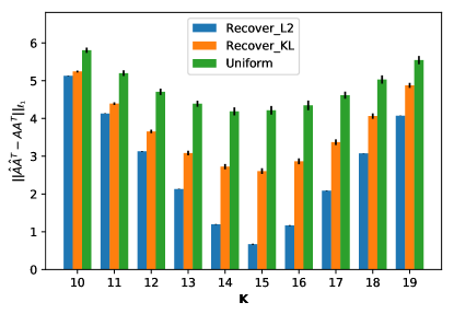
Figure 6: Plot of $\|\widehat{A}\widehat{A}^{T}-AA^{T}\|_{1}$ for using different specified $K$. The black vertical bars are standard errors over 50 datasets.

Comparison of different algorithms for small $K$

We compare Top10, Recover-L2, Recover-KL and T-score in the benchmark setting $N=n=1500$, $p=1000$ and $\xi=1/p$, but for small values of $K$. T-score is the procedure of Ke and Wang (2017), who kindly made the code available to us. Since $K$ is small, the cardinality of each column $W_{i}$ of $W$ is randomly sampled from $\{1,2,3\}$.

In the first experiment, we considered $K=5$ and varied $|I_{k}|$ within $\{2,3,4,5,6\}$. The estimation error $L_{1}(\widehat{A},A)/K$, averaged over $50$ generated datasets, is shown in Figure 7. We see that the performance of Recover-KL is as good as Top10 and even better for $|I_{k}|\leq 3$. However, as already verified in Section 6, Recover-KL has the worst performance for large $K$ and is computationally demanding. The plot also demonstrates that T-score needs at least $4$ anchor words per group in order to have comparable performance with Top10 and Recover-KL. This is as expected since $|I_{k}|$ needs to grow as $p^{2}\log^{2}(n)/(nN)$ in Ke and Wang (2017).

In the second experiment, we set $|I_{k}|=p/100$ and varied $K$ from $\{5,6,\ldots,10\}$. We considered this range of values as, unfortunately, in the implementation of T-score the authors made available to us, it often crashes for $K=11$. The average overall $L_{1}$ estimation error in Figure 7 shows that Top10 has the smallest error over all $K$. T-score has similar performance when $K\leq 8$ but becomes worse than Top10 when $K$ becomes larger.

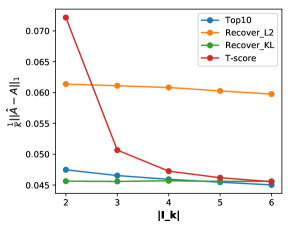
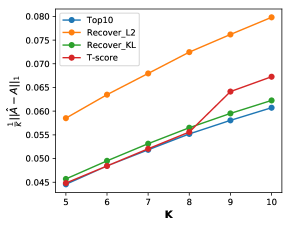
Figure 7: The left plot is the averaged overall estimation error by varying $|I_{k}|$ and setting $K=5$. The right one is for varying $K$ and setting $|I_{k}|=p/100$.

The New York Times (NYT) dataset

Similar to the procedure for preprocessing the NIPs dataset, we removed common stopping words and rare words occurring in less than 150 documents. The dataset after preprocessing has $n=299419$, $p=3079$ and $N=210$. Since Arora et al. (2013) mainly considers $K=100$, we tune our method to obtain a similar number of topics for our comparative study, for both the semi-synthetic data and the real data.

Semi-synthetic data comparison.

To generate the semi-synthetic data, we first apply Top1 to the preprocessed dataset with $C_{0}=0.01$ and $C_{1}=15.5$ and obtain the estimated word-to-topic matrix $\widetilde{A}$ with $\widehat{K}=101$ and $206$ anchor words. Using this $\widetilde{A}$, we generate $W$ from the previous three distributions (a) – (c), separately, with $n=\{40000,50000,60000,70000\}$, and then generate $X$ based on $\widetilde{A}W$ with $N=250$. For each setting, we generate $15$ datasets and the averaged overall estimation error and topic-wise estimation error of Top, Recover-L2, Recover-KL and LDA are reported in Figure 8. The running time of different algorithm is shown in Table 3. We specify the true number of topics for Recover-L2, Recover-KL and LDA while Top estimates it.

The results have essentially the same pattern as those from the NIPs dataset. For the Dirichlet distribution with parameter 0.03, Recover-KL, Recover-L2 and Top are comparable, whereas Top outperforms the other two when the topics become more correlated. LDA has the worst performance, especially when $n$ is relatively small. Top and Recover-L2 run much faster than Recover-KL and LDA.

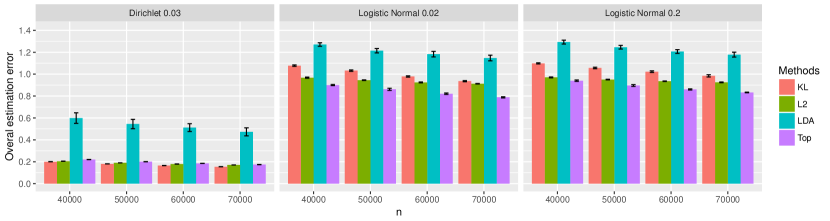
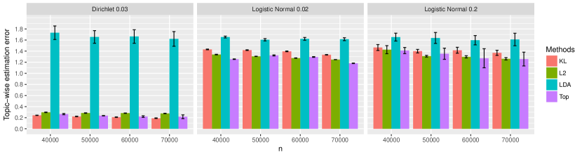
Figure 8: Plots of averaged overall estimation error and topic-wise estimation error of Top, Recover-L2 (L2), Recover-KL (KL) and LDA from the NYT dataset. Top estimates $K$ while the other algorithms use the true $K$ as input. The bars denote one standard deviation.

Table 3: Running time (seconds) of different algorithms on the NYT dataset

	Top	Recover-L2	Recover-KL	LDA
$n=40000$	471.5	795.6	4681.9	35913.7
$n=50000$	517.2	841.5	4824.0	44754.1
$n=60000$	555.3	894.1	4945.3	53833.8
$n=70000$	579.2	957.2	5060.8	62548.8

Real data comparison from the NYT dataset.

We applied Top, Recover-L2, Recover-KL and LDA to the preprocessed NYT dataset. In order to ensure that all algorithms make use of a similar number of topics, Top uses $C_{0}=0.01$ and $C_{1}=15.5$, which gives an estimated $\widehat{K}=101$, and the other three algorithms use $K=101$ as input. Evaluation of algorithms on the real data is difficult since we do not know the ground truth. However, there exists some standard ways of evaluating the fitted model. Since our main target is the word-topic matrix $A$, we consider two widely used metrics of evaluating the semantic quality of estimated topics (Arora et al., 2013; Mimno et al., 2011; Stevens et al., 2012):

1. Topic coherence. Coherence is a measure of the co-occurrence of the high-frequency words for each individual estimated topics. “This metric has been shown to correlate well with human judgments of topic quality. When the topics are perfectly recovered, all the high-probability words in a topic should co-occur frequently, otherwise, the model may be mixing unrelated concepts.” (Arora et al., 2013). Given a set of words $\mathcal{W}$, coherence is calculated as

   $$Coherence(\mathcal{W}):=\sum_{w_{1},w_{2}\in\mathcal{W}}\log{D(w_{1},w_{2})+\varepsilon\over D(w_{2})}$$ (137)

   where $D(w_{1})$ denotes the number of documents that the word $w_{1}$ occurs, $D(w_{1},w_{2})$ denotes the number of documents that both word $w_{1}$ and word $w_{2}$ occur (Mimno et al., 2011) and the parameter $\varepsilon=0.01$ is used to avoid taking the log of zero (Stevens et al., 2012).

   In the NYT dataset, for each algorithm, we use its estimated word-topic matrix $\widehat{A}$ and calculate $Coherence(\mathcal{W}_{k})$ for $1\leq k\leq\widehat{K}$, where $\mathcal{W}_{k}$ is the set of 20 most frequent words in topic $k$. The averaged coherence metrics and its standard deviation across topics of Top, Recover and LDA are reported in Table 4. Top has the largest coherence suggesting a better topic recovery while Recover has the smallest coherence.

2. Unique words: Since coherence only measures the quality of each individual topic, we consider the metric, unique words (Arora et al., 2013), which reflects the redundancy between topics. For each topic and its $T$ most probable words, we count how many of those $T$ words do not appear in any $T$ most probable words of the other topics. Some overlap across topics is expected due to semantic ambiguity, but lower numbers of unique words indicate less useful models. We consider $T=100$ and the averaged unique words and the standard deviation across topics are reported in Table 4. Top and LDA have more unique words than Recover. In fact, the unique words from Recover are only the anchor words and the other most probable words of different topics are all overlapped, indicating the redundancy between the estimated topics.

Table 4: Coherence and unique words of Top, Recover and LDA on the NYT dataset. The numbers in the parentheses are the standard deviations across topics.

Metric	Top	Recover	LDA
Coherence	-328.8(51.3)	-464.1(3.8)	-340.3(44.8)
Unique words	6.7(4.4)	1.0(0.0)	6.3(3.1)

References

- Anandkumar et al. (2012) Anandkumar, A., Foster, D. P., Hsu, D. J., Kakade, S. M. and Liu, Y.-k. (2012). A spectral algorithm for latent dirichlet allocation. In Advances in Neural Information Processing Systems 25 (F. Pereira, C. J. C. Burges, L. Bottou and K. Q. Weinberger, eds.). Curran Associates, Inc., 917–925.
- Arora et al. (2013) Arora, S., Ge, R., Halpern, Y., Mimno, D. M., Moitra, A., Sontag, D., Wu, Y. and Zhu, M. (2013). A practical algorithm for topic modeling with provable guarantees. In ICML (2).
- Arora et al. (2012) Arora, S., Ge, R. and Moitra, A. (2012). Learning topic models–going beyond svd. In Foundations of Computer Science (FOCS), 2012, IEEE 53rd Annual Symposium. IEEE.
- Bansal et al. (2014) Bansal, T., Bhattacharyya, C. and Kannan, R. (2014). A provable svd-based algorithm for learning topics in dominant admixture corpus. In Proceedings of the 27th International Conference on Neural Information Processing Systems - Volume 2. NIPS’14, MIT Press, Cambridge, MA, USA.
- Bing et al. (2017) Bing, X., Bunea, F., Yang, N. and Wegkamp, M. (2017). Sparse latent factor models with pure variables for overlapping clustering. arXiv: 1704.06977 .
- Bittorf et al. (2012) Bittorf, V., Recht, B., Re, C. and Tropp, J. A. (2012). Factoring nonnegative matrices with linear programs. arXiv:1206.1270 .
- Blei (2012) Blei, D. M. (2012). Introduction to probabilistic topic models. Communications of the ACM 55 77–84.
- Blei and Lafferty (2007) Blei, D. M. and Lafferty, J. D. (2007). A correlated topic model of science. Ann. Appl. Stat. 1 17–35.
- Blei et al. (2003) Blei, D. M., Ng, A. Y. and Jordan, M. I. (2003). Latent dirichlet allocation. Journal of Machine Learning Research 993–1022.
- Cox and Reid (1987) Cox, D. R. and Reid, N. (1987). Parameter orthogonality and approximate conditional inference. Journal of the Royal Statistical Society. Series B (Methodological) 49 1–39.
- Deerwester et al. (1990) Deerwester, S., Dumais, S. T., Furnas, G. W., Landauer, T. K. and Harshman, R. (1990). Indexing by latent semantic analysis. Journal of the American society for information science 41 391–407.
- Dheeru and Karra Taniskidou (2017) Dheeru, D. and Karra Taniskidou, E. (2017). UCI machine learning repository.
-
Ding et al. (2013)
Ding, W., Rohban, M. H., Ishwar, P. and
Saligrama, V. (2013).
Topic discovery through data dependent and random projections.
In Proceedings of the 30th International Conference on
Machine Learning (S. Dasgupta and D. McAllester, eds.), vol. 28 of
Proceedings of Machine Learning Research. PMLR, Atlanta, Georgia,
USA.
URL http://proceedings.mlr.press/v28/ding13.html - Donoho and Stodden (2004) Donoho, D. and Stodden, V. (2004). When does non-negative matrix factorization give a correct decomposition into parts? In Advances in Neural Information Processing Systems 16 (S. Thrun, L. K. Saul and P. B. Schölkopf, eds.). MIT Press, 1141–1148.
- Griffiths and Steyvers (2004) Griffiths, T. L. and Steyvers, M. (2004). Finding scientific topics. Proceedings of the National Academy of Sciences 101 5228–5235.
- Hofmann (1999) Hofmann, T. (1999). Probabilistic latent semantic indexing. Proceedings of the Twenty-Second Annual International SIGIR Conference .
- Ke and Wang (2017) Ke, T. Z. and Wang, M. (2017). A new svd approach to optimal topic estimation. arXiv:1704.07016 .
- Li and McCallum (2006) Li, W. and McCallum, A. (2006). Pachinko allocation: Dag-structured mixture models of topic correlations. In Proceedings of the 23rd International Conference on Machine Learning. ICML 2006, ACM, New York, NY, USA.
- Mimno et al. (2011) Mimno, D., Wallach, H. M., Talley, E., Leenders, M. and McCallum, A. (2011). Optimizing semantic coherence in topic models. In Proceedings of the Conference on Empirical Methods in Natural Language Processing. EMNLP ’11, Association for Computational Linguistics, Stroudsburg, PA, USA.
- Papadimitriou et al. (2000) Papadimitriou, C. H., Raghavan, P., Tamaki, H. and Vempala, S. (2000). Latent semantic indexing: A probabilistic analysis. Journal of Computer and System Sciences 61 217–235.
- Papadimitriou et al. (1998) Papadimitriou, C. H., Tamaki, H., Raghavan, P. and Vempala, S. (1998). Latent semantic indexing: A probabilistic analysis. In Proceedings of the Seventeenth ACM SIGACT-SIGMOD-SIGART Symposium on Principles of Database Systems. PODS ’98, ACM, New York, NY, USA.
-
Riddell et al. (2016)
Riddell, A., Hopper, T. and Grivas, A. (2016).
lda: 1.0.4.
URL https://doi.org/10.5281/zenodo.57927 - Stevens et al. (2012) Stevens, K., Kegelmeyer, P., Andrzejewski, D. and Buttler, D. (2012). Exploring topic coherence over many models and many topics. In Proceedings of the 2012 Joint Conference on Empirical Methods in Natural Language Processing and Computational Natural Language Learning. Association for Computational Linguistics, Jeju Island, Korea.
- Tsybakov (2009) Tsybakov, A. B. (2009). Introduction to Nonparametric Estimation. Springer, New York.