3D billiards: visualization of regular structures and trapping of chaotic trajectories

Abstract

The dynamics in three-dimensional $(\textsc{3d})$ billiards leads, using a Poincaré section, to a four–dimensional map which is challenging to visualize. By means of the recently introduced 3d phase-space slices an intuitive representation of the organization of the mixed phase space with regular and chaotic dynamics is obtained. Of particular interest for applications are constraints to classical transport between different regions of phase space which manifest in the statistics of Poincaré recurrence times. For a 3d paraboloid billiard we observe a slow power-law decay caused by long-trapped trajectories which we analyze in phase space and in frequency space. Consistent with previous results for 4d maps we find that: (i) Trapping takes place close to regular structures outside the Arnold web. (ii) Trapping is not due to a generalized island-around-island hierarchy. (iii) The dynamics of sticky orbits is governed by resonance channels which extend far into the chaotic sea. We find clear signatures of partial transport barriers. Moreover, we visualize the geometry of stochastic layers in resonance channels explored by sticky orbits.

I Introduction

Billiard systems are Hamiltonian systems playing an important role in many areas of physics. They are given by the free motion of a point particle moving along straight lines inside some Euclidean domain with specular reflections at the boundary. The dynamics is studied in much detail KozTre1991 ; Tab1995 ; CheMar2006 and ranges from integrable motion, e.g. for billiards in a circle, ellipse or rectangle, to fully chaotic dynamics, e.g. for the Sinai–billiard Sin1970 , the Bunimovich stadium billiard Bun1979 , or the cardioid billiard Rob1983 ; Woj1986 ; Mar1988 ; BaeDul1997 .

Of particular interest is the generic situation with a mixed phase space in which regular motion and chaotic motion coexist MarMey1974 . This occurs for example when the billiard is convex and the boundary is sufficiently smooth, e.g. a slight deformation of the circle such as the family of limaçon billiards Rob1983 ; DulBae2001 . For the class of mushroom billiards a sharply divided mixed phase space is rigorously proven Bun2001 . Billiards also are important model systems in quantum chaos Sto2007b ; Haa2010 and have applications in optical microcavities for which the classical dynamics allows for understanding and tuning directed laser emission GmaCapNarNoeStoFaiSivCho1998 ; CaoWie2015 .

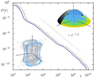
Figure 1: Poincaré recurrence statistics $P(t)$ in the 3d billiard, defined in Eq. (3), for real flight time (red dashed line) and number of mappings (blue line). The dotted line indicates a power-law decay $\sim t^{-\gamma}$ with $\gamma=1.2$. Upper inset: 3d paraboloid billiard shown with part of boundary removed for visual reasons. Inside a sticky trajectory (blue line) is shown which starts and returns to region $\Lambda$ (yellow ring). Lower inset: trapped orbit (blue dots) and regular phase space structures (gray) in a 3d phase-space slice representation.

Three-dimensional $(\textsc{3d})$ billiards (see the upper right inset in Fig. 1 for an illustration) have in particular been investigated for establishing fully chaotic dynamics Bun1988 ; Woj1990 ; BunCasGua1996 ; BunReh1997 ; BunReh1998 ; BunReh1998b ; Bun2000 ; BunMag2006 ; Woj2007 ; RapRomTur2007 ; Sza2017 , and studying both classical and quantum properties of integrable, mixed and fully chaotic systems, see e.g. ZasStr1992 ; PriSmi1995 ; PriSmi2000 ; AltGraHofRanRehRicSchWir1996 ; Pro1997a ; Pro1997b ; Sie1998 ; Kni1998 ; WaaWieDul1999 ; Pap2000 ; Pap2000b ; PapPro2000 ; DemDieGraHeiPapRicRic2002 ; DieMoePapReiRic2008 ; CasRam2011 ; GilSan2011 . Recent applications are in the context of three-dimensional optical micro-cavities MekNoeCheStoCha1995 ; RakYanMcCDonPerMooGapRog2003 ; ChiDumFerFerJesNunPelSorRig2010 ; KreSinHen2017 . Three-dimensional billiards are also of conceptual interest because for systems with more than two degrees-of-freedom new types of transport are possible, including the famous Arnold diffusion Arn1964 ; Chi1979 ; Loc1999 ; Dum2014 .

To understand the dynamics of billiards with a mixed phase space, for 2d billiards the dynamics in the four–dimensional phase space is conveniently reduced to a 2d area–preserving map using energy conservation and a Poincaré section. This can be easily visualized and used for interactive computer explorations, see e.g. Bae2007c . In contrast, for 3d billiards the phase space is six–dimensional and, by energy conservation and a Poincaré section, a 4d symplectic map is obtained, which is difficult to visualize. One method is to use the recently introduced 3d phase-space slice representation to visualize the regular structures of 4d symplectic maps RicLanBaeKet2014 , e.g. of two coupled standard maps Fro1972 . By this approach it is possible to obtain a good overview of regular phase space structures and to demonstrate the generalized island-around-island hierarchy LanRicOnkBaeKet2014 and the organization in terms of families of elliptic 1d tori OnkLanKetBae2016 .

Another motivation comes from the important question on possible (partial) barriers limiting the transport between different regions in phase space in higher-dimensional systems. A sensitive measure for this is the statistics of Poincaré recurrence times $P(t)$. Fully chaotic systems typically show a fast exponential decay, see e.g. BauBer1990 ; ZasTip1991 ; HirSauVai1999 ; AltSilCal2004 , while for systems with a mixed phase space the decay of $P(t)$ is much slower, usually following a power-law ChaLeb1980 ; ChiShe1983 ; Kar1983 ; ChiShe1984 ; KayMeiPer1984a ; HanCarMei1985 ; Mei1986 ; MeiOtt1985 ; MeiOtt1986 ; ZasEdeNiy1997 ; BenKasWhiZas1997 ; ChiShe1999 ; ZasEde2000 ; WeiHufKet2003 ; CriKet2008 ; CedAga2013 ; AluFisMei2014 ; AluFisMei2017 . For recent results on the recurrence time statistics in integrable systems see DetMarStr2016 . Closely related to studying the Poincaré recurrence statistics is the survival probability in open billiards, see e.g. AltTel2008 ; AltTel2009 ; AltPorTel2013 ; DetRah2014 .

For two-dimensional systems the mechanism of the power-law decay of the Poincaré recurrence statistics $P(t)$ is well understood: here 1d regular tori are absolute barriers to the motion and thus separate different regions in phase space. Broken regular tori, so-called cantori, form partial barriers allowing for a limited transport Aub1978 ; Per1980 ; BenKad1984 ; KayMeiPer1984a ; KayMeiPer1984b ; Wig1990 ; RomWig1990 ; RomWig1991 ; Mei1992 ; Mei2015 . Near a regular island formed by invariant Kolmogorov-Arnold-Moser (KAM) curves, there is a whole hierarchy associated with the boundary circle GreMacSta1986 and islands-around-islands Mei1986 . These hierarchies of partial barriers are the origin of sticky chaotic trajectories in the surrounding of a regular island and lead to a power-law behavior of the Poincaré recurrence statistics $P(t)$, see Refs. HanCarMei1985 ; MeiOtt1985 ; MeiOtt1986 ; CriKet2008 ; AluFisMei2017 , and the reviews Mei1992 ; Mei2015 .

For higher-dimensional systems a power-law decay of the Poincaré recurrence statistics is also commonly observed, see e.g. KanKon1989 ; KonKan1990 ; DinBouOtt1990 ; ChiVec1993 ; ChiVec1997 ; AltKan2007 ; ShoLiKomTod2007b ; She2010 ; LanBaeKet2016 and Fig. 1 for an illustration. However, an understanding as in the case of two-dimensional systems is still lacking. The main reason is that, for example for a 4d map, the regular tori are two-dimensional and therefore cannot separate different regions in the 4d phase space. Thus broken regular 2d tori alone cannot form a partial barrier limiting transport.

In this paper we visualize the dynamics of 3d billiards using the 3d phase-space slice representation and based on this investigate stickiness of chaotic orbits. Using the 3d phase-space slice reveals how the regular region is organized around families of elliptic 1d tori and how uncoupled and coupled resonances govern the regular structures in phase space. These can be related to trajectories in configuration space and the representation of the regular region in frequency space. The Poincaré recurrence statistics shows an overall power-law decay. To investigate this decay, one representative long-trapped orbit is analyzed in detail in the 3d phase-space slice and in frequency space. We confirm the findings of Ref. LanBaeKet2016 for a 4d map also in the case of a 3d billiard: (i) Trapping takes place close to regular structures outside the Arnold web. (ii) Trapping is not due to a generalized island-around-island hierarchy. (iii) The dynamics of sticky orbits is governed by resonance channels which extend far into the chaotic sea. Clear signatures of partial barriers are found in frequency space and phase space. Moreover, we visualize the geometry of stochastic layers in resonance channels explored by sticky orbits.

This paper is organized as follows: The first aim is to obtain a visualization of the mixed phase of a generic 3d billiard. For this we briefly introduce in Sec. II.1 billiard systems, the Poincaré section, and as specific example the 3d paraboloid billiard. In Sec. II.2 we review and illustrate 3d phase-space slices and compare with trajectories in configuration space. The representation in frequency space is discussed in Sec. II.3. The generalized island-around-island hierarchy is discussed in Sec. II.4 and properties of resonance channels in Sec. II.5. Understanding the transport in a higher-dimensional system is the second aim of this paper. For this the Poincaré recurrence statistics is introduced and numerical results for the 3d paraboloid billiard are presented in Sec. III.1. The origin of the algebraic decay of the Poincaré recurrence statistics are long-trapped orbits, which we analyze in detail in Sec. III.2 using different representations in phase space and in frequency space.

II Visualizing the dynamics of 3D billiards

II.1 Billiard dynamics and Poincaré section

A 3d billiard system is given as autonomous Hamiltonian system

$$H\left(\mathbf{p},\mathbf{q}\right)=\begin{cases}\mathbf{p}^{2},&\mathbf{q}\in\Omega\\ \infty,&\mathbf{q}\in\partial\Omega\>,\\ \end{cases}\quad$$ (1)

which describes the dynamics of a freely moving point particle within a closed domain $\Omega\subset\mathbb{R}^{3}$ with specular reflections at the boundary $\partial\Omega$. The boundary ${\partial\Omega=\cup_{i=1}^{n}\partial\Omega_{i}}$ is assumed to consist of a finite number of piece-wise smooth elements $\partial\Omega_{i}$. Every point $\mathbf{q}\in\partial\Omega$ has a unique inward pointing unit normal vector $\hat{\mathbf{n}}\left(\mathbf{q}\right)$, except for intersections of boundary elements.

After the free propagation inside the domain the particle collides at a specific point $\mathbf{q}\in\partial\Omega$ with the boundary. With respect to the normal vector $\hat{\mathbf{n}}\left(\mathbf{q}\right)$ the normal projection of the momentum vector changes its sign, while the tangent component remains the same. Therefore the new momentum $\mathbf{p^{\prime}}$ after a reflection is given by

$$\mathbf{p^{\prime}}=\mathbf{p}-2\,\left(\mathbf{p}\cdot\hat{\mathbf{n}}\left(\mathbf{q}\right)\right)\;\hat{\mathbf{n}}\left(\mathbf{q}\right),$$ (2)

where $\mathbf{p}$ is the momentum before the reflection.

The dynamics of a 3d billiard takes place in a 6d phase space with coordinates $\left(p_{x},p_{y},p_{z},x,y,z\right)$. As the Hamiltonian (1) is time–independent, energy is conserved, i.e. $H\left(\mathbf{p},\mathbf{q}\right)$ is constant so that the dynamics takes place on a 5d sub-manifold of constant energy. As the character of the dynamics does not depend on the value of $\|\mathbf{p}\|$, we fix the energy shell by requiring $\|\mathbf{p}\|=1$. A further reduction is obtained by introducing a Poincaré section. This leads to a discrete-time billiard map on a 4d phase space. A good parametrization of the section depends on the considered billiard. Note that for 2d billiards the phase space is four-dimensional and the whole boundary $\partial\Omega$ usually provides a good section. Here the section is conveniently parametrized in Birkhoff coordinates Bir1966 by the arc-length along the boundary and the projection of the (unit) momentum vector onto the unit tangent vector in the point of reflection. In these coordinates one obtains a 2d area-preserving map Bir1966 .

As an explicit example we consider the 3d paraboloid billiard whose domain is defined by a downwards opened paraboloid $\partial\Omega_{1}$ cut by the plane $z=0$, leading to an ellipsoid surface as boundary $\partial\Omega_{2}$,

$$\partial\Omega_{1}=\left\{z=1-\frac{1}{2}\left(\left(\frac{x}{a}\right)^{2}+\left(\frac{y}{b}\right)^{2}\right),\>z\geq 0\right\}$$ (3)

$$\partial\Omega_{2}=\left\{z=0,\>\frac{1}{2}\left(\left(\frac{x}{a}\right)^{2}+\left(\frac{y}{b}\right)^{2}\right)\leq 1\right\},$$

with parameters $a=1.04$ and $b=1.12$. These parameters are chosen such that the billiard has no rotational symmetry, $a\neq b$, and that the central periodic orbit (going along the line $x=0$, $y=0$) is stable as $a,b>1$. The shape of the system is illustrated in the upper inset in Fig. 1 and in Fig. 4 where only one half of the paraboloid $\partial\Omega_{1}$ is drawn and $\partial\Omega_{2}$ is shown in green and yellow. Note that for $a=b$ the $z$ component of the angular momentum is conserved. Numerically this billiard allows for a particularly convenient implementation as reflection points can be computed by solving a quadratic equation Hig2002 .

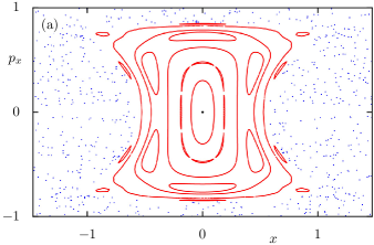
((a))

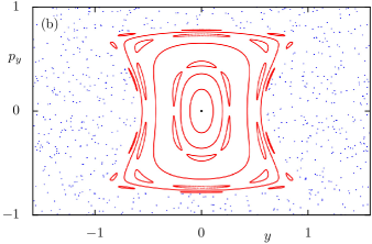
((b))

Figure 2: Phase space for the two 2d billiards embedded in the 3d paraboloid billiard. Regular tori (red rings) are arranged around an elliptic fixed point (black dot) in the center ${{\mathbf{u}_{\mathrm{fp}}^{\textsc{2d}}}=\left(0,0\right)}$. The regular island is embedded in the chaotic region, for which one chaotic orbit is shown (blue dots). (a) For $a=1.04$ two resonances ${8\!:\!3}$ and ${3\!:\!1}$ within the regular region and one ${10\!:\!3}$ resonance at the edge of the regular island are shown. (b) For $b=1.12$ two resonances ${3\!:\!1}$ and ${10\!:\!3}$ within the regular region and one ${14\!:\!4}$ resonance at the edge of the island are shown.

As Poincaré section we choose the plane $z=0$, so that an initial condition is uniquely specified by its location $(x,y)$ within the ellipse $\partial\Omega_{2}$ and the momentum components $\left(p_{x},p_{y}\right)$ since the third component follows from momentum conservation $\|\mathbf{p}\|=1$. This reduces the 3D billiard flow with 6d phase space to a symplectic Poincaré map $\left(p_{x},p_{y},x,y\right)\mapsto\left(p_{x}^{\prime},p_{y}^{\prime},x^{\prime},y^{\prime}\right)$ on a 4d phase space,

$$M=\{ (p_{x},p_{y},x,y)\;|\;(x,y)\in\partial\Omega_{2},$$ (4)

$$(p_{x},p_{y})\in\mathbb{R}^{2}\text{ with }p_{x}^{2}+p_{y}^{2}\leq 1\}$$

with invariant measure $\text{d}\mu=\frac{1}{|\partial\Omega_{2}|\pi}\,\text{d}p_{x}\text{d}p_{y}\text{d}x\text{d}y$. Note that the trajectory can be reflected several times at the curved boundary $\partial\Omega_{1}$ before returning to $\partial\Omega_{2}$. There are two different time measures, namely the number $t$ of applications of the Poincaré map and the real flight time $\tau$, which is the sum of the geometric lengths between consecutive reflections at the billiard boundary $\partial\Omega$.

Let us first discuss two special cases for the dynamics of the 3d paraboloid billiard. Corresponding to the motion in the $x$-$z$ and the $y$-$z$ plane there are two embedded 2d billiards with boundary given by a straight line and parabola with parameters $a$ and $b$, respectively. The central periodic orbit has perpendicular reflections at the boundaries and geometric length 2. As $a,b>1$, the radius of curvature is larger than $1$ and thus larger than half of the length of the periodic orbit so that in both cases the central periodic orbit is stable. The phase space of the corresponding billiard maps in $\left(x,p_{x}\right)$ and $\left(y,p_{y}\right)$, respectively, is shown in Fig. 2.

For the billiard map the stable periodic orbit corresponds to an elliptic fixed point at the center ${{\mathbf{u}_{\mathrm{fp}}^{\textsc{2d}}}=(q_{i},p_{i})=(0,0)}$, indicated as black dot in Fig. 2(a,b). As follows from KAM theory Poe2001 ; Lla2001 ; Dum2014 these elliptic points are surrounded by invariant regular tori, shown as red rings. Between these KAM tori of sufficiently irrational rotation frequency one has nonlinear $r:s$ resonance chains, as implied by the Poincaré-Birkhoff theorem Poi1912 ; Bir1913 , leading to small embedded sub-islands. Note that we choose the numbers $r$ and $s$ such that $r$ is the number of sub-islands of a resonance. The phase space of the billiard map in $\left(x,p_{x}\right)$, see Fig. 2(a), shows a prominent ${6\!:\!2}$ and a smaller ${8\!:\!3}$ resonance near the fixed point. Further outside a ${10\!:\!3}$ resonance is visible. Note that the ${6\!:\!2}$ resonance chain consists of two symmetry-related ${3\!:\!1}$ resonance chains which only differ in the sign of the initial momentum $p_{x}$. For the billiard system in $\left(y,p_{y}\right)$, see Fig. 2(b), there is a ${3\!:\!1}$ resonance near the fixed point and further outside a ${10\!:\!3}$ and a ${14\!:\!4}$ resonance. For both 2d billiards, the central regular island is embedded in a chaotic sea with irregular motion (blue dots in Fig. 2). The central island is enclosed by a last invariant torus called boundary circle GreMacSta1986 .

Note that for both 2d billiards continuous families of marginally unstable periodic orbits exist in the chaotic part of phase space at $p_{i}=0$ AltMotKan2005 ; TanShu2006 ; DetGeo2011 ; BunVel2012 . Such families are not of relevance for our study, as they are part of the recurrence region $\Lambda$ for the Poincaré recurrence statistics discussed in Sec. III.

Considering the dynamics of the 3d billiard, beyond the 2d invariant planes, we have to investigate the full 4d phase space. The central invariant object is the elliptic-elliptic fixed point ${{\mathbf{u}_{\mathrm{fp}}}=(p_{x},p_{y},x,y)=(0,0,0,0)}$ resulting from a direct product of the fixed points ${\mathbf{u}_{\mathrm{fp}}^{\textsc{2d}}}$ of the two 2d billiards. In the neighborhood of this elliptic-elliptic fixed point there is a high density of regular 2d tori DelGut1996 . The regular 2d tori form a whole “regular region”, similar to the regular islands in the 2d billiards. However, note that this regular region is not a connected region but just a collection of regular tori, permeated by chaotic trajectories on arbitrarily fine scales, see Sec. II.5 for a more detailed discussion.

II.2 3D phase space slice

Since a direct visualization of the 4d phase space of the Poincaré section of the three-dimensional billiard is not possible, we use a 3d phase-space slice RicLanBaeKet2014 which is defined using a 3d hyperplane in the 4d phase space. Specifically we choose in the following

$$\Gamma_{\varepsilon}=\left\{(p_{x},p_{y},x,y)\;\left|\rule{0.0pt}{10.33327pt}\;|p_{y}|\leq\varepsilon\right.\right\}$$ (5)

with $\varepsilon=10^{-4}$. Whenever a point $(p_{x},p_{y},x,y)$ of an orbit lies within $\Gamma_{\varepsilon}$, the remaining coordinates $(p_{x},x,y)$ are displayed in a 3d plot. Objects of the 4d phase space usually appear in the 3d phase-space slice with a dimension reduced by one. Thus, a typical 2d torus leads to a pair (or more) of 1d lines. The (numerical) parameter $\varepsilon$ defines the resolution of the resulting 3d phase-space slice. For smaller $\varepsilon$ longer trajectories have to be computed to obtain the same number of points in $\Gamma_{\varepsilon}$. For further illustrations and discussions of the 3d phase-space slice representation see Refs. RicLanBaeKet2014 ; LanRicOnkBaeKet2014 ; OnkLanKetBae2016 ; AnaBouBae2017 .

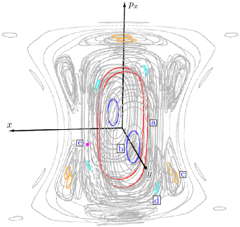
Figure 3: 3d phase-space slice of the billiard defined in Eq. (3) with $a=1.04$ and $b=1.12$ for $|p_{y}|\leq\varepsilon=10^{-4}$. Regular tori appear as 1d lines (gray). For the labeled tori ( a – e ) the corresponding trajectories in configuration space are shown in Fig. 4. For a rotating view see http://www.comp-phys.tu-dresden.de/supp/.

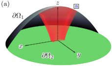
((a))

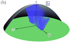
((b))

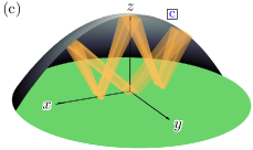
((c))

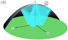
((d))

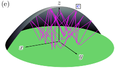
((e))

Figure 4: 3d paraboloid billiard with boundaries $\partial\Omega_{2}$ (green) and $\partial\Omega_{1}$ for which only the part with $y<0$ and trajectories in configuration space for the highlighted tori shown in Fig. 3. a Trajectory (red) close to ${\cal M}_{x}^{\mathrm{fp}}$. b Trajectory (blue) close to ${\cal M}_{y}^{\mathrm{fp}}$. c Trajectory (orange) of an uncoupled resonance related to the billiard system with $a=1.04$. d Trajectory (cyan) of a coupled resonance. e Periodic trajectory (pink) of a double resonance with period $35$.

Fig. 3 shows a 3d phase-space slice representation for the 3d paraboloid billiard. For this a few representative selected initial conditions on regular tori are iterated until $5000$ points fulfill the slice condition (5). Regular 2d tori appear as two (or more) distinct rings, see the colored and labeled tori a – d in Fig. 3. Note that the reflection symmetry of the 3d billiard at the $x$-$z$ plane leads to a symmetry in the 3d phase-space slice with respect to $x$-$p_{x}$ plane. The reflection symmetry at the $y$-$z$ plane corresponds to a symmetry in the 3d phase-space slice with respect to the $y$-$p_{x}$ plane.

All regular tori are embedded in a chaotic sea (not shown), similar to the 2d case in Fig. 2. Thus, the chaotic sea is a 4d volume in phase space and appears as a 3d volume in the 3d phase-space slice.

The 3d phase-space slice representation resembles in large parts the 2d phase space $(x,p_{x})$ of the 2d billiard shown in Fig. 2(a). This results from the chosen slice condition (5), $|p_{y}|\leq\varepsilon$. Alternatively one could consider the slice condition $|p_{x}|\leq\varepsilon$ and display the remaining coordinates $(x,y,p_{y})$. This would resemble in large parts the 2d phase space $(y,p_{y})$ of the 2d billiard shown in Fig. 2(b).

To obtain a better intuition of the 3d phase-space slice we relate some regular 2d tori of Fig. 3 to the corresponding trajectories in configuration space, see Fig. 4:

a The pair of red rings correspond to a regular 2d torus in the 4d phase space and in configuration space to the trajectory shown in Fig. 4(a). This trajectory is close to the $x$-$z$ plane and may be considered as continuation of a trajectory of the 2d billiard dynamics shown in Fig. 2(a) with additional dynamics in $y$-direction.

b For the 2d torus shown in Fig. 4(b) the trajectory is close to the $y$-$z$ plane and therefore similar to the 2d billiard dynamics shown in Fig. 2(a) with additional dynamics in $x$-direction.

c The six orange rings correspond to the trajectory of Fig. 4(c), which is located in the $3:1$ island chain of Fig. 2(a), again with additional dynamics in $y$-direction. Note that this trajectory has a symmetry related partner, which is obtained by inverting the initial momentum. In the 3d phase-space slice this corresponds to the symmetry with respect to the reflection at the $x$-$y$ plane.

d A type of dynamics only occurring in 3d billiards is the cyan 2d torus shown in Fig. 3 with trajectory displayed in Fig. 4(d). Here the coupling between both degrees of freedom can be nicely seen in the twisting envelope of the trajectory in configuration space. Note that this 2d torus has a symmetry-related partner obtained by inverting the initial momentum, i.e. in configuration space one obtains the same type of trajectory passed in opposite sense. In the 3d phase-space slice the symmetry related orbit is obtained by reflection at the $x$-$p_{x}$ plane.

e Moreover, there are also trajectories of the type shown in Fig. 4(e). This is a periodic orbit with period $35$ extending in both degrees of freedom and corresponds to a double resonance (see Sec. II.3), which is not possible in a 2d billiard.

The regular 2d tori in the phase space of a 4d map are organized around families of elliptic 1d tori LanRicOnkBaeKet2014 ; OnkLanKetBae2016 . Most prominently one has the so-called Lyapunov families JorVil1997 ; JorVil1997b ; JorOll2004 of elliptic 1d tori which emanate from the central elliptic-elliptic fixed point ${\mathbf{u}_{\mathrm{fp}}}$. For the 3d billiard these two families ${\cal M}_{x}^{\mathrm{fp}}$ and ${\cal M}_{y}^{\mathrm{fp}}$ corresponds to the regular dynamics of the two embedded 2d billiards shown in Fig. 2. These two families of elliptic 1d tori form a “skeleton” around which the regular 2d tori are organized. For example, the orbit shown in Fig. 4(a) is a regular 2d torus which is close to the Lyapunov family ${\cal M}_{x}^{\mathrm{fp}}$, while the orbit in Fig. 4(b) is close to the Lyapunov family ${\cal M}_{y}^{\mathrm{fp}}$.

In the chosen 3d phase-space slice (5) the family ${\cal M}_{x}^{\mathrm{fp}}$ is completely contained in the $x$-$p_{x}$ plane of Fig. 3. Note that only a few selected trajectories of Fig. 2(a) are displayed. In contrast ${\cal M}_{y}^{\mathrm{fp}}$ coincides with the $y$-axis which is easily seen by applying the slice condition (5) to the phase space shown in Fig. 2(b). The closeness of the 2d tori shown in Fig. 4(a) to ${\cal M}_{x}^{\mathrm{fp}}$ and in Fig. 4(b) to ${\cal M}_{y}^{\mathrm{fp}}$ is also clearly seen in the 3d phase-space slice in Fig. 3. Note that in general the Lyapunov families not necessarily coincide with conjugate variables of the system, see e.g. LanRicOnkBaeKet2014 .

II.3 Frequency space

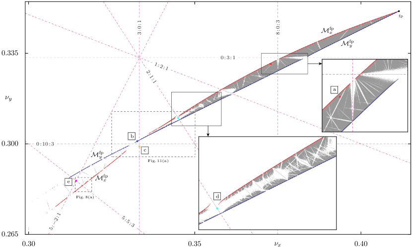
Figure 5: Frequency space of the 3d paraboloid billiard defined in Eq. (3) for $a=1.04$ and $b=1.12$. In total $9.6\times 10^{6}$ frequencies $(\nu_{x},\nu_{y})$ for the 2d tori are displayed (gray points). The rightmost tip $({\nu_{x}^{\mathrm{fp}}},{\nu_{y}^{\mathrm{fp}}})=(0.41143,0.35130)$ corresponds to the elliptic-elliptic fixed point ${\mathbf{u}_{\mathrm{fp}}}$. Two Lyapunov families of elliptic 1d tori ${\cal M}_{x}^{\mathrm{fp}}$ (red) and ${\cal M}_{y}^{\mathrm{fp}}$ (blue) emanate from this point. Some important resonance lines are shown as magenta dashed lines. The insets show magnifications of the frequency space. Colored points marked by a – e correspond to the examples shown in Fig. 3 and Fig. 4.

The frequency space representation is an important complementary approach for understanding higher-dimensional dynamical systems. The basic idea is to associate with every regular 2d torus in the 4d phase space its two fundamental frequencies $(\nu_{x},\nu_{y})\in[0,1)^{2}$ and display them in a 2d frequency space. Numerically this is done using a Fourier-transform based frequency analysis MarDavEzr1987 ; Las1993 ; BarBazGioScaTod1996 . The mapping from phase space to frequency space allows for explaining features observed in the 3d phase-space slice and identifying resonant motion.

For a given initial condition an orbit segment $\{\left(p_{x}^{j},p_{y}^{j},x^{j},y^{j}\right)\}$ with ${j=0,1,...,N_{\text{seg}}-1}$ is obtained from consecutive iterates of the map. In the following $N_{\text{seg}}=4096$ is used. From this orbit two complex signals $s_{x}^{j}=x^{j}-\text{i}p_{x}^{j}$ and $s_{y}^{j}=y^{j}-\text{i}p_{y}^{j}$ are constructed, and for each signal its fundamental frequencies $\nu_{x}$ and $\nu_{y}$ are calculated. Note that usually the computed frequencies are only defined up to an unimodular transformation DulMei2003 ; GekMaiBarUze2007 ; RicLanBaeKet2014 . For the considered 3d billiard system no transformations have to be applied to get a consistent association in frequency space.

To decide whether the motion for a given initial condition is regular or chaotic, another orbit segment $\{\left(p_{x}^{j},p_{y}^{j},x^{j},y^{j}\right)\}$ for $j=N+N_{\text{seg}},...,N+2N_{\text{seg}}-1$ is computed with $N=10^{5}$ giving fundamental frequencies $(\tilde{\nu}_{x},\tilde{\nu}_{y})$. As chaos indicator we use the frequency criterion

$$\delta=\max{\left(|\nu_{x}-\tilde{\nu}_{x}|,|\nu_{y}-\tilde{\nu}_{y}|\right)}<\delta_{\text{reg}}.$$ (6)

This should be close to zero for a regular orbit, while for a chaotic orbit the frequencies of the first and second segment will be very different. While $N=0$ was used in RicLanBaeKet2014 , using $N=10^{5}$ leads to a more sensitive measure, in particular excluding short-time transients. As threshold $\delta_{\text{reg}}=10^{-9}$ has been determined based on a histogram of the $\delta$-values, computed for many initial conditions together with a visual inspection of selected orbits in the 3d phase-space slice. This leads to a total of $9.6\times 10^{6}$ regular tori with corresponding frequency pairs shown in Fig. 5. Based on a visual check using the 3d phase-space slice, initial points for the sampling of the frequency space are chosen within an ellipse $(x,y,z=0)$ with half-axes $r\,a\,\sqrt{2}$, $r\,b\,\sqrt{2}$, and radius $r=0.8$ (see green region in the inset of Fig. 1), and $p_{x}^{2}+p_{y}^{2}\leq 1$. Choosing initial conditions outside of this region leads to chaotic dynamics and thus the frequency criterion (6) is not fulfilled. From the fraction of accepted regular tori the size of the regular region is estimated as $1.4\%$ of the 4d phase space.

Note that even though the frequency criterion (6) is a very sensitive chaos-detector, it uses finite-time information and therefore some of the accepted regular 2d tori are actually chaotic orbits. This is of course common to any tool for chaos detection, see Ref. SkoGotLas2016 for a recent overview.

II.3.1 Regular tori and Lyapunov families

The geometry of the frequency space is governed by a few organizing elements:
First, the frequencies of the central fixed point ${\mathbf{u}_{\mathrm{fp}}}$ can be obtained by a linear stability analysis for each of the two 2d billiards which gives an analytic expression for the frequency of ${\mathbf{u}_{\mathrm{fp}}^{\textsc{2d}}}$ SieSte1990 , evaluating to ${{\mathbf{u}_{\mathrm{fp}}}=({\nu_{x}^{\mathrm{fp}}},{\nu_{y}^{\mathrm{fp}}})\approx(0.41143,0.35130)}$. This point corresponds to the rightmost tip in the frequency plane in Fig. 5.

Second, the two sharp edges (red and blue) emanating from the fixed point correspond to the Lyapunov families of 1d tori ${\cal M}_{x}^{\mathrm{fp}}$ and ${\cal M}_{y}^{\mathrm{fp}}$. For such 1d tori only the longitudinal frequency $\nu_{\text{L}}$, corresponding to $\nu_{x}$ for ${\cal M}_{x}^{\mathrm{fp}}$ and $\nu_{y}$ for ${\cal M}_{y}^{\mathrm{fp}}$, can be determined directly. The other frequency $\nu_{\text{N}}$, called normal or librating frequency, can be computed by contracting a surrounding 2d torus LanRicOnkBaeKet2014 or using a Fourier expansion method JorOll2004 ; CasJor2000 . Going away from the fixed point along the 1d families, i.e. either along ${\cal M}_{x}^{\mathrm{fp}}$ or ${\cal M}_{y}^{\mathrm{fp}}$, corresponds in Fig. 2 to move from the central fixed point ${\mathbf{u}_{\mathrm{fp}}^{\textsc{2d}}}$ towards the boundary of the regular island. For the particular geometry of the 3d paraboloid billiard the Lyapunov families ${\cal M}_{x}^{\mathrm{fp}}$ and ${\cal M}_{y}^{\mathrm{fp}}$ coincide with the dynamics of the 2d billiards shown in Fig. 2.

These lower-dimensional dynamical objects provide the skeleton of the regular dynamics, both in frequency space and in phase space, around which the regular motion on 2d tori is organized. In the vicinity of the fixed point ${\mathbf{u}_{\mathrm{fp}}}$ the frequency pairs of regular 2d tori have a high density and quite densely fill the region between the Lyapunov families, also see upper inset in Fig. 5. With increasing distance from the fixed point, e.g. below $\nu_{x}\approx 0.35$, regular 2d tori only persist close to the families of 1d tori, see the lower inset in Fig. 5. Another important observation are the numerous gaps, i.e. regions not covered by regular tori, which are arranged around straight lines. The origin of these will be discussed in the following section.

II.3.2 Resonance lines

The frequency space is covered by resonance lines, on which the frequencies fulfill the resonance condition

$$m_{x}\nu_{x}+m_{y}\nu_{y}=n$$ (7)

for $m_{x},m_{y},n\in\mathbb{Z}$ without a common divisor and at least $m_{x}$ or $m_{y}$ different from zero. In the following a resonance condition is denoted as ${m_{x}:m_{y}:n}$ and the order of a resonance is given by ${|m_{x}|+|m_{y}|}$. The resonance lines form a dense resonance web in frequency space. Some selected resonance lines are shown in Fig. 5.

For a given frequency pair $(\nu_{x},\nu_{y})$ the number of independent resonance conditions, the so-called rank, determines the type of motion occurring in 4d maps Tod1994 ; Tod1996 (also see LanRicOnkBaeKet2014 for an illustration):

• If the frequency pair fulfills no resonance condition, it is of rank-0 and the motion on the corresponding 2d torus is quasi-periodic, filling it densely. Such frequencies for example correspond to KAM tori of sufficiently incommensurate frequencies. Examples are the red ( a ) and blue ( b ) marked points which correspond to the tori in 3d phase-space slice shown in Fig. 3 and the trajectories in Fig. 4(a) and Fig. 4(b).

• If only one resonance condition is fullfilled (rank-1 case), the resonance is either (a) uncoupled, i.e. ${m_{x}\!:\!0\!:\!n}$ or ${0:m_{y}:n}$, or (b) coupled, i.e. ${m_{x}\!:\!m_{y}\!:\!n}$ with both $m_{x}$ and $m_{y}$ non-zero. The motion is quasi-periodic on a 1d invariant set which either consists of one component in the case of coupled resonances, or of $m_{x}$ (or $m_{y}$) dynamically connected components in the case of uncoupled resonances. Note that in this rank-1 case one has (at least) one pair of elliptic and hyperbolic 1d tori OnkLanKetBae2016 .

  An example of an uncoupled resonance is the orange marked frequency pair $(\nu_{x},\nu_{y})=(0.3333,0.2989)$ located on the ${3\!:\!0\!:\!1}$ resonance line, corresponding to the orange torus of Fig. 3 and the trajectory in Fig. 4(c).

  An example of a coupled resonance is the cyan frequency pair $(\nu_{x},\nu_{y})=(0.3450,0.3099)$ located on the ${2\!:\!1\!:\!1}$ resonance line, corresponding to the cyan colored torus in Fig. 3 and the trajectory in Fig. 4(d).

  The difference between uncoupled and coupled resonances can also be seen by 3d projections encoding the value of the projected coordinate by color scale PatZac1994 ; KatPat2011 , see e.g. Fig. 5 in LanRicOnkBaeKet2014 for a detailed illustration.

• If two independent resonance conditions are fulfilled (rank-2 case) one has a double resonance. The frequency pair lies at the intersection of two resonance lines and leads to (at least) four periodic orbits with different possibilities for their stability.

  As an example, we consider the frequency pair $(\nu_{x},\nu_{y})=(\nicefrac{{n_{1}}}{{m_{1}}},\nicefrac{{n_{2}}}{{m_{2}}})=(\nicefrac{{11}}{{35}},\nicefrac{{2}}{{7}})$ in Fig. 5 which is the intersection of the ${5\!:\!5\!:\!3}$ and ${5\!:\!-2\!:\!1}$ resonance line. The period is given by $\text{lcm}(m_{1},m_{2})=35$. The corresponding elliptic-elliptic trajectory is shown in configuration space in Fig. 4(e).

Resonances also lead to gaps within the areas covered by regular 2d tori, see e.g. the white regions in Fig. 5. Of particular strong influence are resonances of low order as they typically lead to the largest gaps. When resonance lines intersect the families of 1d tori, this also leads to gaps within these families. So strictly speaking, they form one-parameter Cantor families of 1d tori JorVil1997 ; JorVil2001 . If either $|m_{x}|\leq 2$ (for ${\cal M}_{x}^{\mathrm{fp}}$) or $|m_{y}|\leq 2$ (for ${\cal M}_{y}^{\mathrm{fp}}$) this leads to gaps or strong bends in the corresponding families of 1d tori OnkLanKetBae2016 . For example, due to the ${3\!:\!0\!:\!1}$ resonance there is a large gap in ${\cal M}_{x}^{\mathrm{fp}}$ and due to the ${0\!:\!10\!:\!3}$ resonance a smaller one in ${\cal M}_{y}^{\mathrm{fp}}$. Note that in the case of the considered 3d paraboloid billiard the frequencies of the families of 1d tori cross near these gaps, see Fig. 5.

II.4 Hierarchy

For systems with two degrees of freedom the phase space shows a hierarchy of islands-around-islands on ever finer scale which are organized around elliptic periodic orbits Mei1986 . In higher-dimensional systems the organization of phase space is based on higher-dimensional elliptic objects. For example for a 4d map, families of elliptic 1d tori form the skeleton of surrounding regular 2d tori, as discussed above. Thus the generalization of the island-around-island hierarchy can be fully described in terms of the families of elliptic 1d tori LanRicOnkBaeKet2014 : There are two possible origins of such families which either $\left(\alpha\right)$ emanate from an elliptic-elliptic periodic point or $\left(\beta\right)$ result from a family of broken 2d tori fulfilling a rank-1 resonance condition. For the first case one further distinguishes: $\left(\alpha 1\right)$ the fixed point is either the central elliptic-elliptic fixed point ${\mathbf{u}_{\mathrm{fp}}}$ or it corresponds to an elliptic-elliptic periodic point resulting from a broken 2d torus which fulfills a rank-2 resonance. $\left(\alpha 2\right)$ The families of 1d tori emerge from an elliptic-elliptic periodic point resulting from a broken elliptic 1d torus when its longitudinal frequency $\nu_{\text{L}}=\frac{n}{m}$ fulfills an rank-1 resonance. This corresponds to an intersection of a resonance line with a one-parameter family of elliptic 1d tori.

As this hierarchy of elliptic 1d tori is reflected in the surrounding 2d tori, Figs. 3–5 provide an illustration of the hierarchy:

• $\left(\alpha 1\right)$: a and b are examples for orbits close to ${\cal M}_{x}^{\mathrm{fp}}$ and ${\cal M}_{y}^{\mathrm{fp}}$, respectively, which emanate from the central elliptic-elliptic fixed point ${\mathbf{u}_{\mathrm{fp}}}$. An example of a double resonance is the elliptic-elliptic periodic point shown in e . From this periodic orbit also two Lyapunov families of elliptic 1d tori emerge.

• $\left(\alpha 2\right)$: c is an example in the surrounding of the period-3 island, where one elliptic 1d torus of ${\cal M}_{x}^{\mathrm{fp}}$ with longitudinal frequency $\nu_{\text{L}}=\frac{1}{3}$ fulfills the ${3\!:\!0\!:\!1}$ resonance (rank-1), which gives rise to a period-3 periodic orbit with attached Lyapunov families.

• $\left(\beta\right)$: An example of a two-parameter family of 2d tori fulfilling a rank-1 resonance condition is the ${2\!:\!1\!:\!1}$ resonance, for which d shows one surrounding 2d torus.

Analyzing the dynamics of this hierarchy in frequency space requires an adjusted frequency analysis as the frequencies collapse to either $(\alpha)$ a point or $(\beta)$ a resonance line LanRicOnkBaeKet2014 .

II.5 Resonance channels and Arnold diffusion

Points on a resonance line correspond in phase space either to elliptic 1d tori or the surrounding 2d tori. Thus the one-parameter family of elliptic 1d tori forms the “skeleton” of the so-called resonance channel. The regular part of the resonance channel consists of the elliptic 1d tori and their surrounding 2d tori. The chaotic part of the resonance channel consists of the corresponding hyperbolic 1d tori and the chaotic motion in the stochastic layer, which is associated with the homoclinic tangle of the stable and unstable manifolds of the hyperbolic 1d tori. For a detailed discussion of the geometry of resonance channels in phase space and the relation to bifurcations of families of elliptic 1d tori see OnkLanKetBae2016 .

In these stochastic layers chaotic transport along the resonance channels is possible, which is commonly referred to as Arnold diffusion Arn1964 ; Chi1979 ; Loc1999 ; Dum2014 . As resonance lines cover the whole frequency space densely, all stochastic regions of phase space are connected. Their network within the region of regular tori is referred to as Arnold web.

Perturbing an integrable system, Nekhoroshev theory shows that in the near-integrable regime the speed of Arnold diffusion is exponentially small Nek1977 ; Guz2004 , which makes its numerical detection very difficult. This regime is called Nekhoroshev regime. For stronger perturbations regular tori become sparse and neighboring stochastic layers begin to overlap with much faster transport, in particular across channels. This regime is called Chirikov regime GuzLegFro2002 ; FroLegGuz2006 .

The considered 3d paraboloid billard does not qualify as near-integrable. Still the dynamics within a given resonance channel shows both the behavior of the Nekhoroshev and the Chirikov regime depending on the location along the channel, see e.g. lower inset of Fig. 5: Near the intersection of the resonance line with ${\cal M}_{x}^{\mathrm{fp}}$ or ${\cal M}_{y}^{\mathrm{fp}}$, the stochastic layer is embedded in surrounding regular 2d tori and the chaotic dynamics along the channel should be governed by the slow Arnold diffusion, i.e. this part of the resonance channel belongs to the Nekhoroshev regime. Further along the channel the neighboring regular tori become more sparse and one gets into the Chirikov regime in which the stochastic layers of neighboring resonances overlap. Thus transport across resonance channels becomes possible and is more likely further along the channel. In addition other crossing resonance channels may also be explored by a trajectory started within a stochastic layer.

With this general background in mind it is also possible to represent chaotic trajectories in frequency space and interpret the results: Of course, for chaotic trajectories in a stochastic layer no frequencies exist in the infinite time limit, however it is possible to associate “finite-time” frequencies. For example chaotic trajectories approaching a regular torus also acquire similar frequencies. And for trajectories in a stochastic layer their finite-time frequencies will cover a small region in the surrounding of the corresponding resonance line in frequency space. This will be illustrated and discussed in detail in Sec. III.2.

III Stickiness and power-law trapping

III.1 Poincaré recurrence statistics

In systems with a mixed phase space the transport between different regions can be strongly slowed down by so-called stickiness of chaotic trajectories taking place in the surrounding of regular regions. A convenient approach to characterize stickiness is based on the Poincaré recurrence theorem. It states that for a measure-preserving map with invariant probability measure $\mu$ almost all orbits started in a region $\Lambda$ of phase space will return to that region at some later time Poi1890 . Based on the recurrence times $t_{\text{rec}}(x)$ of orbits with initial conditions $x\in\Lambda$, one obtains the recurrence time distribution

$$\rho(t)=\frac{\mu\left(x\in\Lambda\;|\;t_{\text{rec}}(x)=t\right)}{\mu(\Lambda)}.$$ (8)

The average recurrence time follows from Kac’s lemma Kac1947 ; Kac1959 ; Mei1997 as

$$\langle t_{\text{rec}}\rangle:=\frac{1}{\mu(\Lambda)}\int\limits_{\Lambda}t_{\text{rec}}(x)\;\text{d}\mu=\frac{\mu(M_{\text{acc}})}{\mu(\Lambda)},$$ (9)

where $M_{\text{acc}}$ is the accessible region for orbits starting in region $\Lambda$.

Instead of considering the distribution of recurrence times, it is numerically more convenient to use the Poincaré recurrence statistics, which is the complementary cumulative Poincaré recurrence time distribution,

$$P(t)=\sum_{k=t}^{\infty}\rho(k),$$ (10)

i.e. the distribution of the recurrence times larger than $t$. Initially one has $P(0)=1$ and by definition $P(t)$ is monotonically decreasing. Numerically, the Poincaré recurrence statistics is determined by

$$P\left(t\right)=\frac{N\left(t\right)}{N(0)},$$

where $N(0)$ is the number of trajectories initially started in $\Lambda$ and $N\left(t\right)$ is the number of trajectories which have not yet returned to $\Lambda$ until time $t$.

The nature of the decay of $P(t)$ depends on the dynamical properties of the systems. Fully chaotic systems show an exponential decay BauBer1990 ; ZasTip1991 ; HirSauVai1999 ; AltSilCal2004 whereas generic systems with a mixed phase space typically exhibit a power-law decay ChaLeb1980 ; ChiShe1983 ; Kar1983 ; ChiShe1984 ; KayMeiPer1984a ; KayMeiPer1984b ; HanCarMei1985 ; MeiOtt1985 ; MeiOtt1986 ; ZasEdeNiy1997 ; BenKasWhiZas1997 ; ChiShe1999 ; ZasEde2000 ; WeiHufKet2002 ; WeiHufKet2003 ; CriKet2008 ; CedAga2013 ; AluFisMei2014 ; AluFis2015 ; AluFisMei2017 . Note that considering the Poincaré recurrence statistics with respect to $\Lambda$ can also be seen as an escape experiment from an open billiard so that the decay of $P(t)$ agrees with the decay of the survival probability with trajectories injected in the opening $\Lambda$ AltTel2008 .

To numerically study the Poincaré recurrence statistics the region $\Lambda$ in phase space should fulfill two prerequisites in order to obtain good statistics: First $\Lambda$ should be placed in the chaotic sea far away from the regular region to ensure that trajectories are started outside of the expected sticky region. Second, the volume of $\Lambda$ should be chosen sufficiently large to ensure that non-trapped orbits return quickly enough to avoid unnecessary computations. For the 4d Poincaré map of the 3d billiard we chose

$$\begin{split}\Lambda=&\bigg{\{}\left(p_{x},p_{y},x,y\right):\>\frac{1}{2}\left(\left(\frac{x}{a}\right)^{2}+\left(\frac{y}{b}\right)^{2}\right)>r^{2},\\ &~{}~{}\left(x,y\right)\in\partial\Omega_{2},\text{ and }p_{x}^{2}+p_{y}^{2}\leq 1\bigg{\}}.\end{split}$$ (11)

A point $(p_{x},p_{y},x,y)\in\Lambda$ defines the initial condition $(p_{x},p_{y},p_{z},x,y,z)$ with $z=0$ and $p_{z}>0$ via $||\mathbf{p}||=1$. In configuration space the region $\Lambda$ corresponds to an elliptical ring in the $z=0$ plane, defining the opening in $\partial\Omega_{2}$, marked in yellow in the inset of Fig. 1. This allows for starting trajectories into the billiard under all different angles. After visual inspection of the regular structures with the help of the 3d phase-space slice we choose $r=0.8$ for $\Lambda$, which covers $36\%$ of the 4d phase space of the Poincaré map.

For the determination of the Poincaré recurrence statistics ${N(0)=10^{13}}$ random initial conditions are chosen uniformly in $\Lambda$. For each of them the real flight time and the number of iterations of the Poincaré map are determined until the trajectory returns to $\Lambda$.

In Fig. 1 the Poincaré recurrence statistics for real flight times and the number of mappings is shown. Initially one has approximately an exponential decay for small times up to ${t\lesssim 200}$. This corresponds to chaotic trajectories which are not trapped near any of the regular structures and thus return to $\Lambda$ very quickly. For larger times $P(t)$ exhibits an overall power-law decay ${P(t)\sim t^{-\gamma}}$ with exponent $\gamma\approx 1.2$. The only exception of the straight power-law is a small step for $t\in[10^{6},10^{7}]$ which could be a manifestation of some more restrictive partial barriers. Note that one could also consider other geometries of the opening which only affects the initial exponential decay but not the exponent of the power-law decay Fir2014 . The Poincaré recurrence statistics of the number of mappings $t$ and real flight time $\tau$ are shifted by approximately a factor of $\sim 1.94$ which is close to the geometric length $\tau=2$ of the stable periodic orbit in the center of the billiard.

An interesting application of Kac’s lemma is to estimate the size $\mu(M_{\text{reg}})$ of the regular region $M_{\text{reg}}$, as it was done in Mei1997 for the 2d Hénon map. Using the average recurrence time $\langle t_{\text{rec}}\rangle$ one gets from (9)

$$\mu(M_{\text{reg}})=1-\mu(M_{\text{acc}})=1-\langle t_{\text{rec}}\rangle\mu(\Lambda).$$ (12)

With $\langle t_{\text{rec}}\rangle=2.696$ and $\mu(\Lambda)=0.36$ we obtain $\mu(M_{\text{reg}})=0.029$ which gives an estimate of $2.9\%$ for the size of the regular region in the 4d phase space. This is approximately twice as large as the regular fraction determined using the frequency criterion, see Sec. II.3. Note that using Eq. (12) is expected to provide an upper bound to the size of the regular region, as orbits started in $\Lambda$ explore the chaotic region and thus approach the regular region from the outside. Moreover, there might be chaotic regions which are not accessed at all on the considered time-scales, while initial points in such regions could already be detected as chaotic by the frequency criterion (6). Moreover, the threshold $\delta_{\text{reg}}$ for the frequency criterion has been chosen quite small and relaxing this to $\delta_{\text{reg}}=10^{-7}$ gives comparable results for the size of the regular region.

The overall slow decay in the Poincaré recurrence statistics is due to orbits with large recurrence times $t_{\text{rec}}$. Therefore we want to analyze such long-trapped orbits within the phase space and frequency space introduced in Sec. II.2 and Sec. II.3.

III.2 Long-trapped orbits

To obtain a better understanding of the origin of the observed power-law decay of the Poincaré recurrence statistics we consider one representative example of a long-trapped chaotic orbit in the following. Analyzing this long-trapped orbit both in the 3d phase-space slice and in frequency space allows to draw the following conclusions: Trapping takes place (i) at the ”surface” of the regular region (outside the Arnold web) and is (ii) not due to a generalized island-around-island hierarchy, as discussed in Sec. II.4. We find that the dynamics of long-trapped orbits is (iii) governed by numerous resonance channels which extend far into the chaotic sea. The results suggest to decompose the dynamics in the sticky region into (iii.a) transport across resonance channels and (iii.b) transport along resonance channels. For the transport across resonance we find clear signatures of partial barriers. All these points support the results obtained in Ref. LanBaeKet2016 for the case of the 4d coupled standard map. In particular we obtain a very clear example of the geometry of the trapped orbit in the 3d phase-space slice and its signature in frequency space. Note that we only show one representative orbit here, while the essential features are observed for all of the about 100 orbits we analyzed.

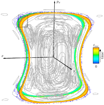
Figure 6: Trapped orbit with recurrence time $t_{\text{rec}}\simeq 1.6\times 10^{9}$ in the 3d phase-space slice representation with time encoded in color. The box indicates the magnification shown in Fig. 7. For a rotating view see http://www.comp-phys.tu-dresden.de/supp/.

To arrive at these conclusions we make use of two time-resolved representations of the long-trapped orbit. In the 3d phase-space slice points of the long-trapped orbit are colored according to time (from blue at $t=0$, starting in $\Lambda$, to orange at $t=t_{\text{rec}}$, returning to $\Lambda$, see colorbar in Fig. 6). It is also possible to analyze trapped orbits in frequency space MarDavEzr1987 ; Las1993 ; ConHarVog2000 ; Lan2016 ; LanBaeKet2016 . Although for chaotic orbits no fundamental frequencies exist, a numerical assignment of frequencies is still possible because for short time intervals the dynamics of nearby regular tori is resembled. For this a sticky chaotic orbit is divided into segments of length $N_{\text{seg}}=4096$. For each segment the frequency analysis, see Sec. II.3, is performed. This leads to a sequence of consecutive frequencies $(\nu_{x}(t_{i}),\nu_{y}(t_{i}))$ with $t_{i}=iN_{\text{seg}}$, $i\in\mathbb{N}$, which can be displayed either in frequency space with time encoded in color or as frequency-time signals, see Fig. 8. Exemplarily, we consider one long-trapped chaotic orbit with large recurrence time $t_{\text{rec}}\simeq 1.6\times 10^{9}$ in the 3d phase-space slice, see Fig. 6 and Fig. 7, and in frequency space, see Fig. 8; another example is discussed in App. B, Fig. 11. Note that these trapped orbits are shown in a 3d phase-space slice with slice parameter $\varepsilon=10^{-3}$, see Eq. (5), to obtain a higher density of points.

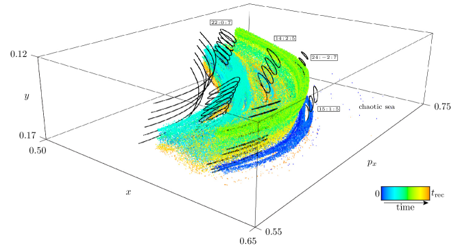
Figure 7: Magnification (rotated) of the trapped orbit of Fig. 6 with recurrence time $t_{\text{rec}}\simeq 1.6\times 10^{9}$ in the 3d phase-space slice with time $[0,t_{\text{rec}})$ encoded in color. Regular tori of some important resonance channels ${22\!:\!0\!:\!7}$, ${14\!:\!2\!:\!5}$, ${24\!:\!-2\!:\!7}$ and ${15\!:\!1\!:\!5}$ are shown in black. The sticky orbit approaches the regular structures by going across several resonance channels. For the time-resolved animation see http://www.comp-phys.tu-dresden.de/supp/.

(i) Trapping is at the surface of the regular region

The long-trapped orbit is shown in the time-encoded 3d phase-space slice in Fig. 6. It is close to the $x$-$p_{x}$ plane and thus close to ${\cal M}_{x}^{\mathrm{fp}}$. The coloring of the orbit according to time shows several bands with different colors, which means that the long-trapped orbit covers different regions of phase space for specific time intervals. Furthermore it is close to regular phase-space structures (gray). More precisely, the orbit is located close to the “surface” of the regular region, which is composed of the regular 2d tori shown as grey rings in the 3d phase-space slice. This is even better seen in a magnified (and rotated) sideways view of the box indicated in the upper left part in Fig. 6. This magnification is shown in Fig. 7, where the surface of the regular region is indicated by the regular 2d tori (black lines) at the left side. Going towards the regular region corresponds to decreasing $x$ and $p_{x}$. The long-trapped orbit arrives from the chaotic see, i.e. from the right in the figure, and approaches the regular region while filling several bands before it returns to the initial region $\Lambda$. An animation of the time-evolution of the long-trapped orbit is provided in the Supplemental Material at http://www.comp-phys.tu-dresden.de/supp/. Further conclusions which can be drawn from this magnification will be discussed below.

In frequency space it can also be seen that the long-trapped orbit is located close to the surface of the regular region: Here the segment-wise determined frequencies of the orbit extend over a large region, see Fig. 8(a), which shows a magnification of the frequency space in Fig. 5 with the frequencies of the trapped orbit colored according to time. Moreover, $9\times 10^{6}$ additional frequency pairs of regular 2d tori are shown (grey dots). The long-trapped orbit spreads approximately parallel to the Lyapunov family ${\cal M}_{x}^{\mathrm{fp}}$, staying above the associated regular tori. Fig. 8(d) shows a magnification of the region indicated in Fig. 8(a), where the ordinate $\tilde{\nu}_{y}$ is the distance to the lower side of the parallelogram, $\tilde{\nu}_{y}=\nu_{y}+k\cdot\nu_{x}+\nu_{s}$ with $k=-0.99$ and $\nu_{s}=0.02925$. Recall that the lower edge (red), which corresponds to the family of 1d tori ${\cal M}_{x}^{\mathrm{fp}}$, can be considered as inner part of the regular region. Thus decreasing $\tilde{\nu}_{y}$ moves towards the surface of the regular region. Moreover, increasing $\nu_{x}$ moves towards the central elliptic-elliptic fixed point. As the sticky orbit stays well outside of any regions with many 2d tori, it is effectively trapped at the surface of the regular region.

In particular this means that it does not enter the Arnold web of resonance lines which are embedded within regular tori.

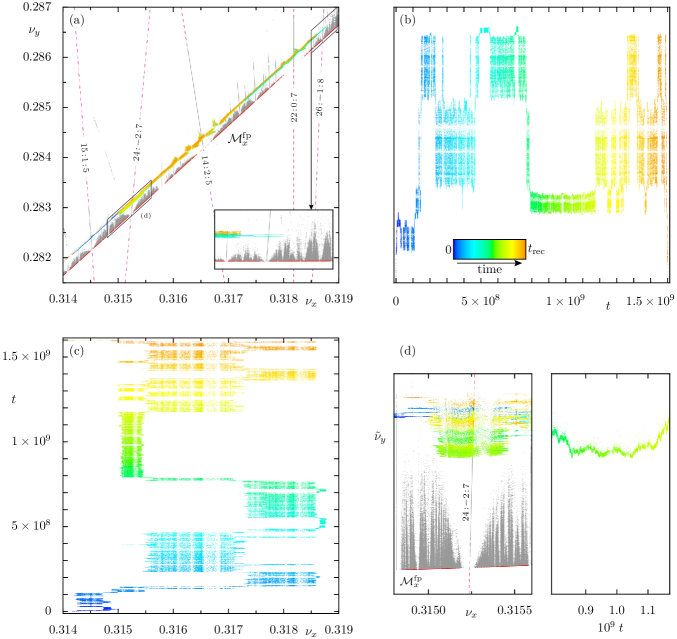
Figure 8: Frequency space representation of the trapped orbit, see Fig. 7, with $t_{\text{rec}}=1.6\times 10^{9}$ and time encoded in color. (a) Magnification of Fig. 5 with regular tori (grey dots) and selected resonance lines, (b, c) frequency-time signals $\nu_{y}(t)$ and $\nu_{x}(t)$, respectively, (d) magnification of frequency-space, see box in (a), in local coordinates.

(ii) Trapping is not due to a hierarchy

Trapping is also not due to the generalized island-around-island hierarchy, summarized in Sec. II.4. This can be concluded from the 3d phase-space slice representation. Trapping deep in a hierarchy would imply successive scaling on finer and finer phase-space structures as known from 2d maps MeiOtt1985 . However, the long-trapped orbit spreads over the surface of the regular region and no signatures of a hierarchy are visible. This is also supported by the frequency-time signals $\nu_{x}(t)$ and $\nu_{y}(t)$ shown in Fig. 8(b, c). For trapping in the generalized hierarchy the frequencies either collapse on a frequency pair $(\alpha_{1})$ or on a resonance line $(\alpha_{2},\beta)$ LanRicOnkBaeKet2014 . Neither of these is observed for the considered example. Note that for the second example of a long-trapped orbit discussed in App. B, the frequency-time signals shown in Fig. 11(b, c) collapse on the ${3\!:\!0\!:\!1}$ resonance for some longer time interval. Still the trapping is not dominated by a hierarchy.

(iii) Resonance channels

The frequency-time signals shown in Fig. 8(b, c) do not collapse on a specific frequency or resonance line but mainly fluctuate within specific frequency ranges over longer time intervals. These frequency ranges are confined around certain resonance lines, as shown in Fig. 8(a), for which ${15\!:\!1\!:\!15}$, ${24\!:\!-2\!:\!7}$, ${14\!:\!2\!:\!5}$, ${22\!:\!0\!:\!7}$, and ${26\!:\!-1\!:\!8}$ are the most important resonances.

These resonance lines correspond to regular dynamics, as discussed in Sec. II.5. Some selected examples of corresponding regular 2d tori are displayed as stacks of black rings in the 3d phase-space slice representation in Fig. 7. For the long-trapped orbit the bands of similarly colored points in the 3d phase-space slice are arranged around these regular parts of the resonance channels. This suggests that the long-trapped orbit is confined to the stochastic layer of the resonance channels.

Both representations and in particular the transformation to local coordinates $(\nu_{x},\tilde{\nu}_{y})$ as shown in Fig. 8(d), together with the animation of the long-trapped orbit in Fig. 7, suggest a decomposition of the chaotic dynamics in transport (iii.a) across and (iii.b) along resonance channels:

(iii.a) In the 3d phase-space slice of Fig. 7 the distinct colored bands indicate that the sticky orbit stays for extended time intervals within the stochastic layer of a given resonance channel, e.g. ${14\!:\!2\!:\!5}$ or ${22\!:\!0\!:\!7}$, and then quickly jumps to a different resonance channel. This happens mainly within the $x$-$p_{x}$ plane, i.e. for approximately constant $y$. These transitions across different resonance channels are also clearly seen in frequency space in Fig. 8(b, c).

(iii.b) Transport along resonance channels is best seen for the ${24\!:\!-2\!:\!7}$ resonance, see the green colored band in Fig. 7, which extends in $y$-direction. In frequency space this corresponds to the magnification shown in Fig. 8(d). We now discuss both types of transport in more detail.

(iii.a) Across resonance channels

In Fig. 8(a) and in particular in the frequency-time signals $\nu_{x}(t)$ and $\nu_{y}(t)$ the importance of four resonance lines namely ${15\!:\!1\!:\!5}$, ${24\!:\!-2\!:\!7}$, ${14\!:\!2\!:\!5}$ and ${22\!:\!0\!:\!7}$ are clearly visible. These resonance lines, together with the surrounding stochastic layers, form the resonance channels which define frequency intervals that are covered in a random looking manner. Furthermore fast transitions to other frequency intervals are observed. The long-trapped orbit is initially, up to $t\approx 10^{8}$, mainly in an interval around the ${15\!:\!1\!:\!5}$ resonance and then up to $t\approx 2.5\times 10^{8}$ around the ${22\!:\!0\!:\!7}$ resonance, followed by a longer time window up to $t\approx 5\times 10^{8}$ around the ${14\!:\!2\!:\!5}$ resonance. Subsequent frequency intervals are around the ${24\!:\!-2\!:\!7}$, ${14\!:\!2\!:\!5}$, and ${22\!:\!0\!:\!7}$ resonance, sometimes with short excursions to the other intervals. The closest approach to the regular region corresponds to the rightmost tip in Fig. 8(a), i.e. largest values of $\nu_{x}$ and $\nu_{y}$ in Fig. 8(b, c). For short time intervals (cyan and green) the small stochastic layer around the ${26\!:\!-1\!:\!8}$ resonance is accessed. Going further to the right is effectively blocked by a region containing many regular 2d tori as indicated in the inset of Fig. 8(a). Even though this region is threaded by resonance lines on arbitrarily fine scales, the effective transport along these lines is expected to be very slow. This is also suggested by the geometry in the 3d phase-space slice, see Fig. 7, where this collection of regular tori constitutes an effective surface.

It is important to emphasize that each stochastic layer actually consists of a whole collection of resonances. For example, the stochastic layer around the ${22\!:\!0\!:\!7}$ resonance corresponds to the whole interval with ${0.3173\lesssim\nu_{x}\lesssim 0.3186}$, see Fig. 8(c). This covers many resonance lines, see the points arranged on lines in Fig. 8(a) which correspond to higher order resonances. Still, the ${22\!:\!0\!:\!7}$ resonance is the most dominant one in this interval as the density of the frequency points $\nu_{x}(t)$ is largest in its surrounding.

The sudden transitions between different frequency intervals are manifestations of partial barriers. For comparison this is illustrated in Appendix A for the 2d billiard shown in Fig. 2(a). There, a sticky orbit approaches the boundary circle in the so-called level hierarchy. In such a two-dimensional case partial barriers are well established as cantorus barriers (broken KAM curves) or broken separatrices formed by stable and unstable manifolds Mei2015 . However, these partial barriers do not generalize to systems with more than two degrees of freedom. Thus by using the frequency analysis it is possible to detect partial barriers without constructing them explicitly, in particular even if their dynamical origin is not known.

These results show that long-trapped orbits explore the chaotic part of resonance channels and jump (iii.a) across resonances, i.e. trapping takes place in the Chirikov regime of overlapping resonances. We find both in frequency space and in phase space clear signatures of some kind of partial transport barriers. At present their dynamical origin is not known.

(iii.b) Along resonance channels

Besides the transport across resonance channels also transport along resonance channels is present. This is best visible for the considered long-trapped orbit around the ${24\!:\!-2\!:\!7}$ resonance, as shown in the magnification in Fig. 8(d). Around the resonance line there is a characteristic triangular-shaped region which is void of any regular 2d tori OnkLanKetBae2016 . The extent is smallest near the Lyapunov family ${\cal M}_{x}^{\mathrm{fp}}$ and widens for increasing $\tilde{\nu}_{y}$. As discussed in Sec. II.5 this corresponds to going from the Nekhoroshev regime, where the channel is surrounded by many regular tori and transport is governed by very slow Arnold diffusion, towards the Chirikov regime of overlapping resonances for which the regular tori are sparse or not present. Thus the distance to ${\cal M}_{x}^{\mathrm{fp}}$ along the resonance channel takes the role of the perturbation strength in the setting of perturbed integrable dynamics. While individual 2d tori in a 4d map cannot confine chaotic motion, a two-parameter family of them (with small gaps due to higher-order resonances) effectively confines the chaotic motion around the resonance within the triangular region in frequency space.

During the time interval $[7.5\times 10^{8},1.1\times 10^{9}]$ the orbit is located in the stochastic layer around the ${24\!:\!-2\!:\!7}$ resonance, i.e. $\nu_{x}{}\in\left[0.315,0.3155\right]$. In the adapted coordinate $\tilde{\nu}_{y}$ one can see that it initially decreases, i.e. the sticky orbit moves along the channel towards the Lyapunov family ${\cal M}_{x}^{\mathrm{fp}}$, see Fig. 8(d). This approach is followed by a longer time-interval with fluctuations around some constant $\tilde{\nu}_{y}$ before the orbit moves along the channel away from the Lyapunov family ${\cal M}_{x}^{\mathrm{fp}}$. The involved time-scales show that the motion along the resonance channel is typically much slower than the motion within the stochastic layer, i.e. see spreading in $\nu_{x}$-direction or animation of Fig. 7.

The numerical results indicate that the transition rates for going across resonance channels depend on the position along a resonance channel, see Fig. 8(d). In the considered time interval the adapted frequency $\tilde{\nu}_{y}$ of the long-trapped orbit first decreases, interpreted as approaching the Nekhoroshev regime in which transitions across resonance channels become unlikely. Subsequently the orbit moves along the channel away from ${\cal M}_{x}^{\mathrm{fp}}$ into the Chirikov regime allowing for transitions across resonance channels. Note that in Ref. LanBaeKet2016 it is suggested that transport along channels can be modeled by a stochastic process with effective drift which gives one possible mechanism of power-law trapping.

Since the Arnold web of connected resonance channels is not explored on the considered time scales, Arnold diffusion is not the origin of the long-trapped orbits.

IV Summary and outlook

In this paper we visualize the mixed phase space of a 3d billiard and analyze restricted classical transport, manifested by a slow decay of the Poincaré recurrence statistics, due to long-trapped orbits. To understand the dynamics of a 3d billiard its 6d phase space is reduced by energy conservation and a Poincaré section to a 4d symplectic map. This 4d map with mixed phase space is visualized using a 3d phase-space slice which reduces the dimension of orbits and invariant objects such that they can be displayed in a 3d plot. This provides a good overview of the regular region and its organization. A complementary representation is the 2d frequency space in which both regular tori and sticky trajectories can be represented and related to resonances. Moreover, the frequency computation provides a chaos indicator to distinguish between regular and chaotic dynamics. The orbits in the 3d phase-space slice and in frequency space can be related to trajectories in configuration space of the 3d billiard which provides an instructive representation of objects in higher-dimensional systems.

The second focus of the paper is to study transport properties. A slow power-law decay of the Poincaré recurrence statistics indicates the presence of sticky orbits. This is of particular interest as the mechanism of stickiness for higher-dimensional systems is still not understood, in contrast to trapping in systems with two degrees of freedom. By analyzing long-trapped orbits in the 3d phase-space slice and in frequency space we find that trapping takes place (i) at the ”surface” of the regular region (outside the Arnold web) and is (ii) not due to a generalized island-around-island hierarchy. We find that the dynamics of long-trapped orbits is (iii) governed by numerous resonance channels which extend far into the chaotic sea. The sticky orbits stay for long times within a stochastic layer of a resonance channel, with fast transitions to other channels. These are clear signatures, that between the stochastic layers there are some restrictive partial barriers, whose dynamical origin is not yet clear. For the 3d billiards the results in the 3d phase-space slice, see Fig. 7 in particular, suggest the existence of an effective (local) boundary surface formed by regular 2d tori which is approached by the sticky chaotic orbits via a sequence of coupled and uncoupled resonances.

An important task for the future is to identify and compute the relevant partial barriers. Based on this it should be possible to define the different states and ultimately explain the origin of power-law trapping in higher-dimensional systems. Another interesting application of the visualization of the phase space of a 3d billiard are 3d optical microcavities where understanding the mixed phase space may guide how to tune their emission patterns.

Appendix A Signatures of partial barriers in 2D billiards

In 2d billiards, and more generally in autonomous Hamiltonian systems with two degrees-of-freedom, the origin for power-law trapping are partial transport barriers Mei1992 ; Mei2015 . We now illustrate how signatures of these partial barriers can be detected in the frequency-time plots for a 2d billiard. This allows for comparing with the corresponding time-frequency plots of the 3d billiard. As an example we consider the 2d billiard shown in Fig. 2(a) and determine the Poincaré recurrence statistics as in Sec. III.1. The result in Fig. 9 shows an overall power-law with exponent $\gamma\approx 1.5$. The slower decay around $t\approx 10^{7}$ is presumably caused by some more restrictive partial barriers.

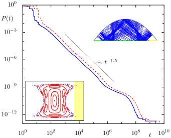
Figure 9: Poincaré recurrence statistics $P(t)$ for the 2d billiard with $a=1.04$ for $10^{13}$ trajectories started in region $\Lambda$ for the number of mappings (blue line) and real flight time (red dashed line). The dotted line indicates a power-law decay $\sim t^{-\gamma}$ with $\gamma=1.5$. Upper inset: opened 2d billiard with parabola as boundary and a short sticky trajectory with ${t_{\text{rec}}=131}$. Lower inset: Poincaré section $(x,p_{x})$ with regular tori (red curves), opening $\Lambda$ (yellow rectangle), and corresponding trapped orbit (blue dots).

Figure 10: (a) Trapped orbit of the 2d billiard with $a=1.04$ with recurrence time $t_{\text{rec}}\simeq 1.52\times 10^{7}$ in a magnification of phase space with time $[0,t_{\text{rec}})$ encoded in color. Additionally shown is the boundary circle (full, black curve) and important surrounding resonances are labeled as fraction $n/m$. For the time-resolved animation see http://www.comp-phys.tu-dresden.de/supp/. (b) Frequency-time representation $\nu(t)$ of the sticky orbit. Frequencies of important resonances are shown as magenta dashed lines and the frequency $\nu_{\text{BC}}$ of the boundary circle as solid horizontal line.

Fig. 10 shows a long-trapped orbit with ${t_{\text{rec}}\simeq 1.52\times 10^{7}}$ and time encoded by color (blue to orange) in a magnification of phase space and in frequency-time representation $\nu(t)$, computed as in section Sec. III.2 from the complex signal $x-\text{i}p_{x}$ for segments of length $N_{\text{seg}}=4096$. In phase space the long-trapped orbit approaches the boundary circle of the central regular island, depicted in an animation of the time-evolution provided in the Supplemental Material at http://www.comp-phys.tu-dresden.de/supp/. The boundary circle is the last invariant curve and thus dynamically separates the regular region from the surrounding chaotic motion. The boundary circle has an irrational frequency $\nu_{\text{BC}}$ which can be approximated by the convergents of its continued fraction expansion GreMacSta1986 . For the boundary circle with frequency $\nu_{\text{BC}}\approx 0.30659$, the first approximants are $\frac{3}{10}$, $\frac{4}{13}$, $\frac{19}{62}$, $\frac{23}{75}$, $\frac{42}{137}$. Note that only every second approximant is smaller than $\nu_{\text{BC}}$, giving the sequence of principal resonances $\frac{3}{10}$, $\frac{19}{62}$, and $\frac{42}{137}$. Each of these fractions corresponds to a resonance chain with elliptic periodic orbits, surrounded by regular motion, and hyperbolic periodic orbits with associated chaotic layer. These chaotic layers correspond to the states in a Markov model description of power-law trapping and separated from each other by partial barriers. These partial barriers are cantori, broken KAM tori, with irrational frequency $\nu_{\text{c}}$ which themselves can be approximated by periodic orbits corresponding to the convergents of the continued fraction expansion of $\nu_{\text{c}}$. The transition rates between the states corresponding to the stochastic layers become smaller and smaller when approaching the boundary circle. A long-trapped orbit is expected to approach the boundary circle via this so-called level hierarchy of such states. Note that the stochastic component of each of these states usually contains several other (non-principal) resonances. Moreover, trapping also takes place in the neighborhood of the resonance islands and their island-around-island hierarchy Mei1986 ; MeiOtt1985 ; WeiHufKet2003 , which leads to time-intervals with constant frequency.

The different stochastic layers correspond to the regions with different colors in Fig. 10(a). Signatures of the partial transport barriers can also be clearly seen in the frequency-time plot. Here the signal $\nu(t)$ randomly fluctuates within some interval around a principal resonant frequency. Passing through a partial barrier, a different frequency interval around another dominant resonance is accessed. For the example shown in Fig. 10(b) the frequencies of the sticky orbit are initially confined in an interval around $\nu=\frac{n}{m}=\frac{49}{160}$ and then a sudden transition to the stochastic layer around $\nu=\frac{19}{62}$ occurs. This is one of the convergents of $\nu_{\text{BC}}$ and is closer to the boundary circle, compare with Fig. 10(a). The stochastic layer around the next convergent $\nu=\frac{42}{137}$ is only accessed very briefly. Finally the level-hierarchy is left via the stochastic layer around $\nu=\frac{49}{160}$ and by passing through $\nu=\frac{15}{49}$ and $\nu=\frac{3}{10}$ (not shown). Note that in this example not only stochastic regions associated with the convergents of the boundary circle, but also several other non-principal resonances and partial barriers appear to be of relevance for the long-time stickiness of the trapped orbit.

Appendix B Further example of a trapped orbit in the 3D billiard

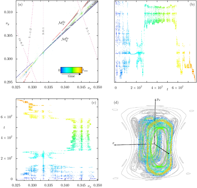
Figure 11: Trapped orbit with recurrence time $t_{\text{rec}}\simeq 7.6\times 10^{7}$ and time $t$ encoded in color. (a) Magnification of Fig. 5 with regular tori (grey dots) and selected resonance lines, (b, c) frequency-time signals $\nu_{y}(t)$ and $\nu_{x}(t)$, (d) 3d phase-space slice representation, for a rotating view see http://www.comp-phys.tu-dresden.de/supp/.

A second example of a long-trapped orbit in the 3d paraboloid billiard is shown in Fig. 11. Both in the 3d phase-space slice and in frequency space, see Fig. 11(a, d), the orbit is located in a different region than the example discussed in Sec. III.2, Figs. 6–8. In particular the plot in frequency space reveals that the sticky orbit is close to the region where ${\cal M}_{x}^{\mathrm{fp}}$ has a gap due to the important ${3\!:\!0\!:\!1}$ resonance and is contained between the stochastic layers of the ${2\!:\!1\!:\!1}$ and the ${7\!:\!1\!:\!2}$ resonance. In the frequency-time plots, Fig. 11(b, c), the orbit first, up to $t\approx 1.3\times 10^{7}$, rapidly jumps between the stochastic layers of these two resonances, and then mainly stays in the stochastic layer of either of them, i.e. for $t\in[3\times 10^{7},5.6\times 10^{7}]$ around the ${2\!:\!1\!:\!1}$ resonance clearly visible as green and yellow colored stochastic layers in the 3d phase-space slice representation in Fig. 11(d). This highlights the possibility that different stochastic layers may either behave as one large stochastic layer or two separate ones.

For this orbit also trapping deeper in the hierarchy is found for the time interval $t\in[1.5\times 10^{7},2.2\times 10^{7}]$ for which in Fig. 11(b, c) the frequency-time signals collapse onto the frequencies of the ${3\!:\!0\!:\!1}$ resonance. Note, that the deeper hierarchy around the ${3\!:\!0\!:\!1}$ resonance is not visible in the chosen perspective.

Thus overall this second example shows both in phase space and in frequency space conceptually the same signatures as the one discussed in Sec. III.2.

References

- (1) V. V. Kozlov and D. V. Treshche̋v, Billiards. A genetic Introduction to the Dynamics of Systems with Impacts, volume 89 of Translations of Mathematical Monographs, American Mathematical Society, Providence, Rhode Island (1991).
- (2) S. Tabachnikov, Billiards, Panoramas et Synthèses 1, Société Mathematique de France, Paris (1995).
- (3) N. Chernov and R. Markarian, Chaotic Billiards, volume 127 of Mathematical Surveys and Monographs, American Mathematical Society, Providence, Rhode Island (2006).
- (4) Ya. G. Sinai, Dynamical systems with elastic reflections, Russ. Math. Surv. 25, 137 (1970).
- (5) L. A. Bunimovich, On the ergodic properties of nowhere dispersing billiards, Commun. Math. Phys. 65, 295 (1979).
- (6) M. Robnik, Classical dynamics of a family of billiards with analytic boundaries, J. Phys. A 16, 3971 (1983).
- (7) M. Wojtkowski, Principles for the design of billiards with nonvanishing Lyapunov exponents, Commun. Math. Phys. 105, 391 (1986).
- (8) R. Markarian, Billiards with Pesin region of measure one, Commun. Math. Phys. 118, 87 (1988).
- (9) A. Bäcker and H. R. Dullin, Symbolic dynamics and periodic orbits for the cardioid billiard, J. Phys. A 30, 1991 (1997).
- (10) L. Markus and K. R. Meyer, Generic Hamiltonian Dynamical Systems are neither Integrable nor Ergodic, number 144 in Mem. Amer. Math. Soc., American Mathematical Society, Providence, Rhode Island (1974).
- (11) H. R. Dullin and A. Bäcker, About ergodicity in the family of limaçon billiards, Nonlinearity 14, 1673 (2001).
- (12) L. A. Bunimovich, Mushrooms and other billiards with divided phase space, Chaos 11, 802 (2001).
- (13) H.-J. Stöckmann, Quantum Chaos: An Introduction, Cambridge University Press, Cambridge (2007).
- (14) F. Haake, Quantum Signatures of Chaos, Springer-Verlag, Berlin, 3rd revised and enlarged edition (2010).
- (15) C. Gmachl, F. Capasso, E. E. Narimanov, J. U. Nöckel, A. D. Stone, J. Faist, D. L. Sivco, and A. Y. Cho, High-power directional emission from microlasers with chaotic resonators, Science 280, 1556 (1998).
- (16) H. Cao and J. Wiersig, Dielectric microcavities: Model systems for wave chaos and non-Hermitian physics, Rev. Mod. Phys. 87, 61 (2015).
- (17) L. A. Bunimovich, Many-dimensional nowhere dispersing billiards with chaotic behavior, Physica D 33, 58 (1988).
- (18) M. P. Wojtkowski, Linearly stable orbits in 3 dimensional billiards, Commun. Math. Phys. 129, 319 (1990).
- (19) L. A. Bunimovich, G. Casati, and I. Guarneri, Chaotic focusing billiards in higher dimensions, Phys. Rev. Lett. 77, 2941 (1996).
- (20) L. A. Bunimovich and J. Rehacek, Nowhere dispersing 3D billiards with non-vanishing Lyapunov exponents, Commun. Math. Phys. 189, 729 (1997).
- (21) L. A. Bunimovich and J. Rehacek, On the ergodicity of many-dimensional focusing billiards, Ann. Inst. Henri Poincaré A 68, 421 (1998).
- (22) L. A. Bunimovich and J. Rehacek, How high-dimensional stadia look like, Commun. Math. Phys. 197, 277 (1998).
- (23) L. A. Bunimovich, Hyperbolicity and astigmatism, J. Stat. Phys. 101, 373 (2000).
- (24) L. A. Bunimovich and G. Del Magno, Semi-focusing billiards: Hyperbolicity, Commun. Math. Phys. 262, 17 (2006).
- (25) M. P. Wojtkowski, Design of hyperbolic billiards, Commun. Math. Phys. 273, 283 (2007).
- (26) A. Rapoport, V. Rom-Kedar, and D. Turaev, Approximating multi-dimensional Hamiltonian flows by billiards, Commun. Math. Phys. 272, 567 (2007).
- (27) D. Szász, Multidimensional hyperbolic billiards, in A. M. Blokh, L. A. Bunimovich, P. H. Jung, L. G. Oversteegen, and Y. G. Sinai (editors) “Dynamical Systems, Ergodic Theory, and Probability: in Memory of Kolya Chernov”, volume 698 of Contemporary Mathematics, American Mathematical Society, Providence, Rhode Island (2017).
- (28) G. M. Zaslavsky and H. R. Strauss, Billiard in a barrel, Chaos 2, 469 (1992).
- (29) H. Primack and U. Smilansky, Quantization of the three-dimensional Sinai billiard, Phys. Rev. Lett. 74, 4831 (1995).
- (30) H. Primack and U. Smilansky, The quantum three-dimensional Sinai billiard – a semiclassical analysis, Phys. Rep. 327, 1 (2000).
- (31) H. Alt, H.-D. Gräf, R. Hofferbert, C. Rangacharyulu, H. Rehfeld, A. Richter, P. Schardt, and A. Wirzba, Chaotic dynamics in a three-dimensional superconducting microwave billiard, Phys. Rev. E 54, 2303 (1996).
- (32) T. Prosen, Quantization of generic chaotic 3d billiard with smooth boundary I. Energy level statistics, Phys. Lett. A 233, 323 (1997).
- (33) T. Prosen, Quantization of generic chaotic 3D billiard with smooth boundary II: Structure of high-lying eigenstates, Phys. Lett. A 233, 332 (1997).
- (34) M. Sieber, Billiard systems in three dimensions: the boundary integral equation and the trace formula, Nonlinearity 11, 1607 (1998).
- (35) O. Knill, On nonconvex caustics of convex billiards, Elem. Math. 53, 89 (1998).
- (36) H. Waalkens, J. Wiersig, and H. R. Dullin, Triaxial ellipsoidal quantum billiards, Ann. Phys. 276, 64 (1999).
- (37) T. Papenbrock, Numerical study of a three-dimensional generalized stadium billiard, Phys. Rev. E 61, 4626 (2000).
- (38) T. Papenbrock, Lyapunov exponents and Kolmogorov-Sinai entropy for a high-dimensional convex billiard, Phys. Rev. E 61, 1337 (2000).
- (39) T. Papenbrock and T. Prosen, Quantization of a billiard model for interacting particles, Phys. Rev. Lett. 84, 262 (2000).
- (40) C. Dembowski, B. Dietz, H.-D. Gräf, A. Heine, T. Papenbrock, A. Richter, and C. Richter, Experimental test of a trace formula for a chaotic three-dimensional microwave cavity, Phys. Rev. Lett. 89, 064101 (2002).
- (41) B. Dietz, B. Mößner, T. Papenbrock, U. Reif, and A. Richter, Bouncing ball orbits and symmetry breaking effects in a three-dimensional chaotic billiard, Phys. Rev. E 77, 046221 (2008).
- (42) P. Casas and R. Ramírez-Ros, The frequency map for billiards inside ellipsoids, SIAM J. Appl. Dyn. Syst. 10, 278 (2011).
- (43) T. Gilbert and D. P. Sanders, Stable and unstable regimes in higher-dimensional convex billiards with cylindrical shape, New J. Phys. 13, 023040 (2011).
- (44) A. Mekis, J. U. Nöckel, G. Chen, A. D. Stone, and R. K. Chang, Ray chaos and spoiling in lasing droplets, Phys. Rev. Lett. 75, 2682 (1995).
- (45) Y. P. Rakovich, L. Yang, E. M. McCabe, J. F. Donegan, T. Perova, A. Moore, N. Gaponik, and A. Rogach, Whispering gallery mode emission from a composite system of CdTe nanocrystals and a spherical microcavity, Semicond. Sci. Technol. 18, 914 (2003).
- (46) A. Chiasera, Y. Dumeige, P. Féron, M. Ferrari, Y. Jestin, G. Nunzi Conti, S. Pelli, S. Soria, and G. Righini, Spherical whispering-gallery-mode microresonators, Laser Photonics Rev. 4, 457 (2010).
- (47) J. Kreismann, S. Sinzinger, and M. Hentschel, Three-dimensional limaçon: Properties and applications, Phys. Rev. A 95, 011801(R) (2017).
- (48) V. I. Arnol’d, Instability of dynamical systems with several degrees of freedom, Sov. Math. Dokl. 5, 581 (1964).
- (49) B. V. Chirikov, A universal instability of many-dimensional oscillator systems, Phys. Rep. 52, 263 (1979).
- (50) P. Lochak, Arnold diffusion; A compendium of remarks and questions, in C. Simó (editor) “Hamiltonian Systems with Three or More Degrees of Freedom”, volume 533 of NATO ASI Series: C - Mathematical and Physical Sciences, 168, Kluwer Academic Publishers, Dordrecht (1999).
- (51) H. S. Dumas, The KAM Story: A Friendly Introduction to the Content, History, and Significance of Classical Kolmogorov–Arnold–Moser Theory, World Scientific, Singapore (2014).
- (52) A. Bäcker, Quantum chaos in billiards, Computing in Science & Engineering 9, 60 (2007).
- (53) M. Richter, S. Lange, A. Bäcker, and R. Ketzmerick, Visualization and comparison of classical structures and quantum states of four-dimensional maps, Phys. Rev. E 89, 022902 (2014).
- (54) C. Froeschlé, Numerical study of a four-dimensional mapping, Astron. & Astrophys. 16, 172 (1972).
- (55) S. Lange, M. Richter, F. Onken, A. Bäcker, and R. Ketzmerick, Global structure of regular tori in a generic 4D symplectic map, Chaos 24, 024409 (2014).
- (56) F. Onken, S. Lange, R. Ketzmerick, and A. Bäcker, Bifurcations of families of 1D-tori in 4D symplectic maps, Chaos 26, 063124 (2016).
- (57) W. Bauer and G. F. Bertsch, Decay of ordered and chaotic systems, Phys. Rev. Lett. 65, 2213 (1990).
- (58) G. M. Zaslavsky and M. K. Tippett, Connection between recurrence-time statistics and anomalous transport, Phys. Rev. Lett. 67, 3251 (1991).
- (59) M. Hirata, B. Saussol, and S. Vaienti, Statistics of return times: A general framework and new applications, Commun. Math. Phys. 206, 33 (1999).
- (60) E. G. Altmann, E. C. da Silva, and I. L. Caldas, Recurrence time statistics for finite size intervals, Chaos 14, 975 (2004).
- (61) S. R. Channon and J. L. Lebowitz, Numerical experiments in stochasticity and homoclinic oscillation, Ann. N.Y. Acad. Sci. 357, 108 (1980).
- (62) B. V. Chirikov and D. L. Shepelyansky, Statistics of Poincaré recurrences and the structure of the stochastic layer of a nonlinear resonance, (1983), in Proceedings of the 9th International Conference on Nonlinear Oscillations, Kiev, 1981; Qualitative methods of the theory of nonlinear oscillators, vol. 2, edited by Yu. A. Mitropolsky, 421–424, Naukova Dumka, Kiev, (1984). English translation: Princeton University Report No. PPPL-TRANS-133 (1983).
- (63) C. F. F. Karney, Long-time correlations in the stochastic regime, Physica D 8, 360 (1983).
- (64) B. V. Chirikov and D. L. Shepelyansky, Correlation properties of dynamical chaos in Hamiltonian systems, Physica D 13, 395 (1984).
- (65) R. S. MacKay, J. D. Meiss, and I. C. Percival, Stochasticity and transport in Hamiltonian systems, Phys. Rev. Lett. 52, 697 (1984).
- (66) J. D. Hanson, J. R. Cary, and J. D. Meiss, Algebraic decay in self-similar Markov chains, J. Stat. Phys. 39, 327 (1985).
- (67) J. D. Meiss, Class renormalization: Islands around islands, Phys. Rev. A 34, 2375 (1986).
- (68) J. D. Meiss and E. Ott, Markov-tree model of intrinsic transport in Hamiltonian systems, Phys. Rev. Lett. 55, 2741 (1985).
- (69) J. D. Meiss and E. Ott, Markov tree model of transport in area-preserving maps, Physica D 20, 387 (1986).
- (70) G. M. Zaslavsky, M. Edelmann, and B. A. Niyazov, Self-similarity, renormalization, and phase space nonuniformity of Hamiltonian chaotic dynamics, Chaos 7, 159 (1997).
- (71) S. Benkadda, S. Kassibrakis, R. B. White, and G. M. Zaslavsky, Self-similarity and transport in the standard map, Phys. Rev. E 55, 4909 (1997).
- (72) B. V. Chirikov and D. L. Shepelyansky, Asymptotic statistics of Poincaré recurrences in Hamiltonian systems with divided phase space, Phys. Rev. Lett. 82, 528 (1999).
- (73) G. M. Zaslavsky and M. Edelmann, Hierarchical structures in the phase space and fractional kinetics: I. Classical systems, Chaos 10, 135 (2000).
- (74) M. Weiss, L. Hufnagel, and R. Ketzmerick, Can simple renormalization theories describe the trapping of chaotic trajectories in mixed systems?, Phys. Rev. E 67, 046209 (2003).
- (75) G. Cristadoro and R. Ketzmerick, Universality of algebraic decays in Hamiltonian systems, Phys. Rev. Lett. 100, 184101 (2008).
- (76) R. Ceder and O. Agam, Fluctuations in the relaxation dynamics of mixed chaotic systems, Phys. Rev. E 87, 012918 (2013).
- (77) O. Alus, S. Fishman, and J. D. Meiss, Statistics of the island-around-island hierarchy in Hamiltonian phase space, Phys. Rev. E 90, 062923 (2014).
- (78) O. Alus, S. Fishman, and J. D. Meiss, Universal exponent for transport in mixed Hamiltonian dynamics, Phys. Rev. E 96, 032204 (2017).
- (79) C. P. Dettmann, J. Marklof, and A. Strömbergsson, Universal hitting time statistics for integrable flows, J. Stat. Phys. 1 (2016), vIP: use DetMarStr2017 as this is only the online published version.
- (80) E. G. Altmann and T. Tél, Poincaré recurrences from the perspective of transient chaos, Phys. Rev. Lett. 100, 174101 (2008).
- (81) E. G. Altmann and T. Tél, Poincaré recurrences and transient chaos in systems with leaks, Phys. Rev. E 79, 016204 (2009).
- (82) E. G. Altmann, J. S. E. Portela, and T. Tél, Leaking chaotic systems, Rev. Mod. Phys. 85, 869 (2013).
- (83) C. P. Dettmann and M. R. Rahman, Survival probability for open spherical billiards, Chaos 24, 043130 (2014).
- (84) S. Aubry, The new concept of transitions by breaking of analyticity in a crystallographic model, in A. R. Bishop and T. Schneider (editors) “Solitons and Condensed Matter Physics”, volume 8 of Springer Series in Solid-State Sciences, 264, Springer Berlin Heidelberg (1978).
- (85) I. C. Percival, Variational principles for invariant tori and cantori, in “AIP Conference Proceedings”, volume 57, 302, AIP Publishing (1980).
- (86) D. Bensimon and L. P. Kadanoff, Extended chaos and disappearance of KAM trajectories, Physica D 13, 82 (1984).
- (87) R. S. MacKay, J. D. Meiss, and I. C. Percival, Transport in Hamiltonian systems, Physica D 13, 55 (1984).
- (88) S. Wiggins, On the geometry of transport in phase space I. Transport in -degree-of-freedom Hamiltonian systems, , Physica D 44, 471 (1990).
- (89) V. Rom-Kedar and S. Wiggins, Transport in two-dimensional maps, Arch. Rational Mech. Anal. 109, 239 (1990).
- (90) V. Rom-Kedar and S. Wiggins, Transport in two-dimensional maps: Concepts, examples, and a comparison of the theory of Rom-Kedar and Wiggins with the Markov model of MacKay, Meiss, Ott, and Percival, Physica D 51, 248 (1991).
- (91) J. D. Meiss, Symplectic maps, variational principles, and transport, Rev. Mod. Phys. 64, 795 (1992).
- (92) J. D. Meiss, Thirty years of turnstiles and transport, Chaos 25, 097602 (2015).
- (93) J. M. Greene, R. S. MacKay, and J. Stark, Boundary circles for area-preserving maps, Physica D 21, 267 (1986).
- (94) K. Kaneko and T. Konishi, Diffusion in Hamiltonian dynamical systems with many degrees of freedom, Phys. Rev. A 40, 6130 (1989).
- (95) T. Konishi and K. Kaneko, Diffusion in Hamiltonian chaos and its size dependence, J. Phys. A 23, L715 (1990).
- (96) M. Ding, T. Bountis, and E. Ott, Algebraic escape in higher dimensional Hamiltonian systems, Phys. Lett. A 151, 395 (1990).
- (97) B. V. Chirikov and V. V. Vecheslavov, Theory of fast Arnold diffusion in many-frequency systems, J. Stat. Phys. 71, 243 (1993).
- (98) B. V. Chirikov and V. V. Vecheslavov, Arnold diffusion in large systems, J. Exp. Theor. Phys. 85, 616 (1997).
- (99) E. G. Altmann and H. Kantz, Hypothesis of strong chaos and anomalous diffusion in coupled symplectic maps, Europhys. Lett. 78, 10008 (2007).
- (100) A. Shojiguchi, C.-B. Li, T. Komatsuzaki, and M. Toda, Fractional behavior in multidimensional Hamiltonian systems describing reactions, Phys. Rev. E 76, 056205 (2007), erratum ibid. 77, 019902(E) (2008).
- (101) D. L. Shepelyansky, Poincaré recurrences in Hamiltonian systems with a few degrees of freedom, Phys. Rev. E 82, 055202(R) (2010).
- (102) S. Lange, A. Bäcker, and R. Ketzmerick, What is the mechanism of power-law distributed Poincaré recurrences in higher-dimensional systems?, EPL 116, 30002 (2016).
- (103) G. D. Birkhoff, Dynamical Systems, volume 9 of Colloquium publications, American Mathematical Society, Providence, Rhode Island, revised edition (1966).
- (104) N. J. Higham, Accuracy and Stability of Numerical Algorithms, Society for Industrial and Applied Mathematics, Philadelphia, PA, USA, second edition (2002).
- (105) J. Pöschel, A lecture on the classical KAM theorem, in A. Katok, R. de la Llave, Y. Pesin, and H. Weiss (editors) “Smooth Ergodic Theory and its Applications”, volume 69 of Proceedings of Symposia in Pure Mathematics, 707, Amer. Math. Soc., Providence, RI (2001).
- (106) R. de la Llave, A tutorial on KAM theory, in A. Katok, R. de la Llave, Y. Pesin, and H. Weiss (editors) “Smooth Ergodic Theory and its Applications”, volume 69 of Proceedings of Symposia in Pure Mathematics, 75–292, Amer. Math. Soc., Providence, RI (2001).
- (107) H. Poincaré, Sur un théorème de géométrie, Rend. Cir. Mat. Palermo 33, 375 (1912).
- (108) G. D. Birkhoff, Proof of Poincaré’s geometric theorem, Trans. Amer. Math. Soc. 14, 14 (1913).
- (109) E. G. Altmann, A. E. Motter, and H. Kantz, Stickiness in mushroom billiards, Chaos 15, 033105 (2005).
- (110) H. Tanaka and A. Shudo, Recurrence time distribution in mushroom billiards with parabolic hat, Phys. Rev. E 74, 036211 (2006).
- (111) C. P. Dettmann and O. Georgiou, Open mushrooms: stickiness revisited, J. Phys. A 44, 195102 (2011).
- (112) L. A. Bunimovich and L. V. Vela-Arevalo, Many faces of stickiness in Hamiltonian systems, Chaos 22, 026103 (2012).
- (113) A. Delshams and P. Gutiérrez, Estimates on invariant tori near an elliptic equilibrium point of a Hamiltonian system, J. Diff. Eqs. 131, 277 (1996).
- (114) S. Anastassiou, T. Bountis, and A. Bäcker, Homoclinic points of 2D and 4D maps via the parametrization method, Nonlinearity 30, 3799 (2017).
- (115) À. Jorba and J. Villanueva, On the normal behaviour of partially elliptic lower-dimensional tori of Hamiltonian systems, Nonlinearity 10, 783 (1997).
- (116) À. Jorba and J. Villanueva, On the persistence of lower dimensional invariant tori under quasi-periodic perturbations, J. Nonlinear Sci. 7, 427 (1997).
- (117) À. Jorba and M. Ollé, Invariant curves near Hamiltonian-Hopf bifurcations of four-dimensional symplectic maps, Nonlinearity 17, 691 (2004).
- (118) C. C. Martens, M. J. Davis, and G. S. Ezra, Local frequency analysis of chaotic motion in multidimensional systems: energy transport and bottlenecks in planar OCS, Chem. Phys. Lett. 142, 519 (1987).
- (119) J. Laskar, Frequency analysis for multi-dimensional systems. Global dynamics and diffusion, Physica D 67, 257 (1993).
- (120) R. Bartolini, A. Bazzani, M. Giovannozzi, W. Scandale, and E. Todesco, Tune evaluation in simulations and experiments, Part. Accel. 52, 147 (1996).
- (121) H. R. Dullin and J. D. Meiss, Twist singularities for symplectic maps, Chaos 13, 1 (2003).
- (122) S. Gekle, J. Main, T. Bartsch, and T. Uzer, Hydrogen atom in crossed electric and magnetic fields: Phase space topology and torus quantization via periodic orbits, Phys. Rev. A 75, 023406 (2007).
- (123) Ch. Skokos, G. A. Gottwald, and J. Laskar (editors) Chaos Detection and Predictability, volume 915 of Lecture Notes in Physics, Springer Berlin Heidelberg (2016).
- (124) M. Sieber and F. Steiner, Classical and quantum mechanics of a strongly chaotic billiard system, Physica D 44, 248 (1990).
- (125) E. Castellá and À. Jorba, On the vertical families of two-dimensional tori near the triangular points of the bicircular problem, Celest. Mech. Dyn. Astron. 76, 35 (2000).
- (126) E. Todesco, Analysis of resonant structures of four-dimensional symplectic mappings, using normal forms, Phys. Rev. E 50, R4298 (1994).
- (127) E. Todesco, Local analysis of formal stability and existence of fixed points in 4d symplectic mappings, Physica D 95, 1 (1996).
- (128) P. A. Patsis and L. Zachilas, Using color and rotation for visualizing four-dimensional Poincaré cross-sections: With applications to the orbital behavior of a three-dimensional Hamiltonian system, Int. J. Bifurcation Chaos 4, 1399 (1994).
- (129) M. Katsanikas and P. A. Patsis, The structure of invariant tori in a 3D galactic potential, Int. J. Bifurcation Chaos 21, 467 (2011).
- (130) À. Jorba and J. Villanueva, The fine geometry of the Cantor families of invariant tori in Hamiltonian systems, in C. Casacuberta, R. Miró-Roig, J. Verdera, and S. Xambó-Descamps (editors) “European Congress of Mathematics”, volume 202 of Progress in Mathematics, 557, Birkhäuser Basel (2001).
- (131) N. N. Nekhoroshev, An exponential estimate of the time of stability of nearly-integrable Hamiltonian systems, Russ. Math. Surv. 32, 1 (1977).
- (132) M. Guzzo, A direct proof of the Nekhoroshev theorem for nearly integrable symplectic maps, Ann. Henri Poincaré 5, 1013 (2004).
- (133) M. Guzzo, E. Lega, and C. Froeschlé, On the numerical detection of the effective stability of chaotic motions in quasi-integrable systems, Physica D 163, 1 (2002).
- (134) C. Froeschlé, E. Lega, and M. Guzzo, Analysis of the Chaotic Behaviour of Orbits Diffusing along the Arnold Web, Celest. Mech. Dyn. Astron. 95, 141 (2006).
- (135) H. Poincaré, Sur le problème des trois corps et les équations de la dynamique, Acta Math. 13, 1 (1890).
- (136) M. Kac, On the notion of recurrence in discrete stochastic processes, Bulletin of the American Mathematical Society 53, 1002 (1947).
- (137) M. Kac, Probability and Related Topics in Physical Sciences, Lectures in Applied Mathematics Series, Vol 1a, American Mathematical Society (1959).
- (138) J. D. Meiss, Average exit time for volume-preserving maps, Chaos 7, 139 (1997).
- (139) M. Weiss, L. Hufnagel, and R. Ketzmerick, Universal power-law decay in Hamiltonian systems?, Phys. Rev. Lett. 89, 239401 (2002).
- (140) O. Alus and S. Fishman, Diffusion for ensembles of standard maps, Phys. Rev. E 92, 042904 (2015).
- (141) M. Firmbach, 3D Billards: Dynamik im gemischten Phasenraum und Potenzgesetz des Hängenbleibens, Bachelor thesis, Technische Universität Dresden, Fachrichtung Physik (2014).
- (142) G. Contopoulos, M. Harsoula, and N. Voglis, Crossing of various cantori, Celest. Mech. Dyn. Astron. 78, 197 (2000).
- (143) S. Lange, Chaotic transport and trapping close to regular structures in 4D symplectic maps, Ph.D. thesis, Technische Universität Dresden, Fachrichtung Physik (2016).
- (144) P. Ramachandran and G. Varoquaux, Mayavi: 3D visualization of scientific data, Comput. Sci. Eng. 13, 40 (2011).