Local vertex corrections from exchange-correlation kernels with a discontinuity

Abstract

The fundamental gap of an interacting many-electron system is given by the sum of the single-particle Kohn-Sham gap and the derivative discontinuity. The latter can be generated by advanced approximations to the exchange-correlation (XC) energy and is the key quantity to capture strong correlation with density functional theory (DFT). In this work we derive an expression for the derivative discontinuity in terms of the XC kernel of time-dependent density functional theory and demonstrate the crucial role of a discontinuity in the XC kernel itself. By relating approximate XC kernels to approximate local vertex corrections we then generate beyond-GW self-energies that include a discontinuity in the local vertex function. The quantitative importance of this result is illustrated with a numerical study of the local exchange vertex on model systems.

I Introduction

Kohn-Sham (KS) density functional theory (DFT) is the most widely used many-electron approach for numerical simulations in physics, chemistry and materials science. kohnsham1965 ; rg84 In both its static and time-dependent (TD) version, the interacting many-electron problem is reformulated into the simpler problem of non-interacting electrons moving in a self-consistent, single-particle KS potential. This construction is formally exact, but is expected to become more constrained when the electrons are strongly correlated. On the other hand, exact studies on simple systems have shown that the KS potential captures effects of strong correlation by exhibiting rather intuitive peak and step features. stepsbarth ; perdewsteps ; gritsenko ; helbigsteps ; TDSTEPS ; hodgson17 Standard local and semi-local approximations to the exchange-correlation (XC) energy, such as LDA and GGA functionals, miss these features and, as a consequence, tend to spread out or delocalize the electrons in the system.

In a seminal work of Perdew et al.pplb82 it was shown that a key feature of the exact XC energy functional is a derivative discontinuity (DD) at integer particle numbers. The DD corrects the largely underestimated single-particle KS gap, and prevents delocalization through the formation of discontinuous XC steps in the KS potential. To capture strong correlation with (TD)DFT it is thus necessary to construct functionals with the DD. It should be noted that the concept of strong correlation can be ambiguous since it sometimes refers to effects beyond semi-local approximations in DFT and sometimes to multi-reference effects beyond Hartree-Fock (HF). In the first case the DD can often be captured by local exact-exchange,kli92 ; hg13 hybridbecke or corrective DFT+U functionals.dftu In the latter, truly correlated case, the DD constitute the entire gap, and it still remains a challenge to find approximate functionals.

Approximations based on many-body perturbation theory (MBPT) have shown to successfully capture many effects of correlation such as screening, van der Waals forces and derivative discontinuities derived from nonlocal exchange. One example is the random phase approximation (RPA), derived from the GW self-energy within MBPT. The RPA and the GW approximation (GWA) share many virtues but both fail in describing localized states in strongly correlated systems such as Mott insulators. hrg12 ; GWRPA1 ; GWRPA ; colonna2 The GWA can be improved by including so-called vertex corrections. So far a HF-like vertex has been employed to construct various total energy expressions based on partial re-summations of particle-hole diagrams. doi:10.1063/1.3250347 ; PhysRevB.88.035120 ; PhysRevB.92.081104 ; toulouse_prl ; RPAx-F Similarly, approximations based on the local exact-exchange vertex was studied in Refs. hvb10, ; hesselmann_random_2010, ; PhysRevB.90.125150, ; gorlingrpax, . Local vertex corrections have also been studied at the simpler level of LDA. delsolevertex Improved local vertex corrections can be derived from improved XC kernels within TDDFT. grosskohn ; bruneval The XC kernel is defined as the functional derivative of the XC potential with respect to the density and is the crucial quantity to calculate excitation energies within linear response TDDFT. pgg96 Recently, it was shown that also the XC kernel exhibits discontinuities at integer particle number, important for charge-transfer excitationshg12 ; hg13 and chemical reactivity indices. hgjcp12

In this work we will investigate the effects of the discontinuity of the XC kernel for constructing local vertex corrections to the many-body self-energy. It has, e.g., previously been shown that affinities need a three-point vertex to be accurately described. localvertexromaniello Here we show that this problem can reformulated into the problem of a missing dynamical discontinuity of the two-point XC kernel. From the ACFD (adiabatic connection fluctuation dissipation) expression to the total energy we further derive an exact expression to the fundamental gap in terms of the XC kernel and its corresponding discontinuity. Finally, we calculate the discontinuity of the exact-exchange kernel and use it to determine correlated gaps beyond the GWA.

II Derivative discontinuity in (TD)DFT

In this section we review some of the mathematical formulas underlying the concept of the DD in static and time-dependent DFT.

The DD refers to a discontinuous change in the derivative of the XC energy, $E_{\rm xc}$, as the density passes integer particle numbers. As a consequence, the corresponding XC potential, $v_{\rm xc}$, jumps with a space-independent constant. The DD has been proven to be a feature of the exact theory, pplb82 ; sagvolden ; cohenmori09 ; SCEDD and to play a key role when applying (TD)DFT to different physical problems such as, e.g., charge-transfer processes, Kondo or Coulomb blockade phenomena. TDSTEPS ; hg12 ; CBDD ; SFIDD ; KONDO1 ; KONDO2 ; CTDD The most direct effect of the discontinuity is, however, seen when trying to extract the fundamental gap from DFT. The ionization energy $I$ and the affinity $A$ of a system with $N_{0}$ particles can be calculated as the left and right derivatives of the total energy with respect to particle number $N$, i.e,

$$-I=\left.\frac{\partial E}{\partial N}\right|_{-},\,\,\,\,\,-A=\left.\frac{\partial E}{\partial N}\right|_{+}$$ (1)

where the subscript $\pm$ refers to the value of the quantity at $N^{\pm}_{0}=N_{0}+0^{\pm}$. The ionization energy of the KS system is equal to the ionization energy of the true interacting system almbarth but the KS affinity $A_{s}$ has to be corrected with the discontinuity ${\rm\Delta}_{\rm xc}$ of the XC potential. The gap of the interacting system is thus equal to the KS gap plus the discontinuity, i.e.,

$$I-A=I-A_{s}+{\rm\Delta}_{\rm xc}.$$ (2)

It has been demonstrated that the DD is comparable in size to the KS gap for both solids gunnshon ; gruning06 and molecules. gapsfinite2 ; gapsfinite Moreover, in strongly correlated Mott insulators the discontinuity accounts for the entire gap. yangscience ; lorenzana

Following Ref. hg12, we will now derive a formal expression for the quantity ${\rm\Delta}_{\rm xc}$ which is useful for extracting the discontinuity of approximate functionals. Using the chain rule we can write the partial derivative of $E_{\rm xc}$ with respect to $N$ as

$$\frac{\partial E_{{\rm xc}}}{\partial N}=\int\!d{\bf r}\,v_{{\rm xc}}({\bf r})\frac{\partial n({\bf r})}{\partial N}.$$ (3)

In the limit $N_{0}^{-}=N_{0}+0^{-}$ this expression can be rewritten as

$$0=\left.\frac{\partial E_{{\rm xc}}}{\partial N}\right|_{-}-\int\!d{\bf r}\,v^{-}_{{\rm xc}}({\bf r})f^{-}({\bf r}),$$ (4)

where $f({\bf r})=\partial n({\bf r})/\partial N$ is the so-called Fukui function. fukui1 ; Fukui Let us now look at the right derivative of $E_{\rm xc}$, which will be different from the left derivative if a DD is present. From Eq. (3) we see that this difference can appear either in the XC potential $v^{+}_{{\rm xc}}({\bf r})=v^{-}_{{\rm xc}}({\bf r})+{\rm\Delta}_{\rm xc}$ or in the Fukui function. In fact, it is easy to see that in the case of local or semilocal functionals such as LDA and PBE the discontinuous behaviour is restricted to the Fukui function, i.e., ${\rm\Delta}_{\rm xc}=0$. Meta-GGAs have shown to exhibit a discontinuity in the XC potential, albeit very small. eichhellgren On the other hand, orbital functionals based on MBPT are known to accurately capture the discontinuity of the XC potential.

Let us now write $v_{\rm xc}({\bf r})=v^{-}_{\rm xc}({\bf r})+{\rm\Delta}_{\rm xc}({\bf r})$ and cast Eq. (3) into

$$\int\!d{\bf r}\,{\rm\Delta}_{\rm xc}({\bf r})f({\bf r})=\frac{\partial E_{{\rm xc}}}{\partial N}-\int\!d{\bf r}\,v^{-}_{{\rm xc}}({\bf r})f({\bf r}).$$ (5)

In the limit $N\rightarrow N_{0}^{+}$, ${\rm\Delta}_{\rm xc}({\bf r})\to{\rm\Delta}_{\rm xc}$ and we find an expression for the discontinuity of $v_{\rm xc}$

$${\rm\Delta}_{\rm xc}=\left.\frac{\partial E_{{\rm xc}}}{\partial N}\right|_{+}-\int\!d{\bf r}\,v^{-}_{{\rm xc}}({\bf r})f^{+}({\bf r}).$$ (6)

A systematic scheme for generating orbital functionals based on MBPT was presented in Ref. vbdvls05, . The idea is to start from variational energy expressions of the Green’s function $G$ and then restrict the variational freedom to Green’s functions $G_{s}$ coming from a local KS potential. One can, for example, start from the Klein functional klein

$$E[G] = -i{\rm\Phi}[G]+E_{\rm H}+i{\rm Tr}\,[GG_{s}^{-1}-1+\ln(-G^{-1})],$$ (7)

which contains another functional ${\rm\Phi}$ having the property that the self-energy ${\rm\Sigma}$ is generated as ${\rm\Sigma}=\delta{\rm\Phi}/\delta G$. When restricting to KS Green’s functions it is easy to see that the XC energy corresponds to $E_{\rm xc}=-i{\rm\Phi}[G_{s}]$. Furthermore, the equation for the XC potential is nothing but the linearized Sham-Schlüter (LSS) equation sham ; shams ; godbylss ; godbylss2 ; casida95

$$\int\!d2\,\chi_{s}(1,2)v_{\rm xc}(2)=\int\!d2d3\,{\rm\Sigma}_{\rm xc}(2,3){\rm\Lambda}(3,2;1).$$ (8)

Here we have simplified the notation by introducing $1={\bf r}_{1},t_{1}$. Even with the exact self-energy this scheme will never be exact but it has shown to produce useful approximations such as the exact-exchange (EXX) approximation (based on the HF self-energy) and the random phase approximation (RPA) (based on the GW self-energy). To determine the discontinuities of the Klein XC potentials, Eq. (7) and Eq. (8) must be generalized to ensemble Green’s functions. This was done in Refs. hg12, ; hrg12, showing that the discontinuities of the Klein functional are given by

$${\rm\Delta}_{\rm xc} = \int\!d{\bf r}d{\bf r}^{\prime}\,\varphi^{*}_{\rm L}({\bf r}){\rm\Sigma}^{+}_{{\rm xc}}({\bf r},{\bf r}^{\prime},\varepsilon^{+}_{\rm L})\varphi_{\rm L}({\bf r}^{\prime})$$ (9)

$$\,\,\,-\int\!d{\bf r}\,v^{-}_{{\rm xc}}({\bf r})|\varphi_{\rm L}({\bf r})|^{2}.$$

where $\rm L$ signifies the LUMO (lowest unoccupied molecular orbital). The superscript on the self-energy can be dropped as it is, in general, invariant with respect to a constant shift of the potential. Combining Eq. (9) with Eq. (2) leads to

$$-A=\varepsilon^{-}_{\rm L}+{\rm\Delta}_{\rm xc}=\varepsilon^{-}_{\rm L}+\langle\varphi_{\rm L}|{\rm\Sigma}_{\rm xc}(\varepsilon_{\rm L})-v^{-}_{\rm xc}|\varphi_{\rm L}\rangle$$ (10)

where the KS LUMO is calculated from $v^{-}_{\rm xc}$. This equation is very similar to the first order quasi-particle equation within MBPT.

The above mathematical analysis was restricted to the static case but also the time-dependent $v_{\rm xc}$ exhibits jumps. In the linear response regime this leads to a frequency and space-dependent discontinuity in the XC kernel given by

$$f^{+}_{\rm xc}({\bf r},{\bf r}^{\prime},\omega)=f^{-}_{\rm xc}({\bf r},{\bf r}^{\prime},\omega)+g_{\rm xc}({\bf r},\omega)+g_{\rm xc}({\bf r}^{\prime},\omega).$$ (11)

In order to determine the discontinuity $g_{\rm xc}({\bf r},\omega)$ of the XC kernel, given an approximation to $v_{\rm xc}$, we use a similar procedure as in the static case but with a generalized ensemble that allow densities to change particle number in time. In Ref. hg12, it was shown that such an ensemble was necessary for functional derivatives to be uniquely defined.

Assuming that $v_{\rm xc}$ is defined on such a generalised domain of densities we can evaluate the functional derivative of $v_{\rm xc}$ with respect to the time-dependent number of particles, i.e.,

$$\left.\frac{\delta v_{\rm xc}({\bf r}t)}{\delta N(t^{\prime})}\right|_{n^{+}_{0}} = \int\!d{\bf r}^{\prime}\,f^{-}_{\rm xc}({\bf r},{\bf r}^{\prime},t-t^{\prime})f^{+}({\bf r}^{\prime})$$ (12)

$$\!\!\!\!\!\!\!\!\!\!\!\!\!\!\!\!\!\!\!\!\!\!+\int\!d{\bf r}^{\prime}\,g_{\rm xc}({\bf r}^{\prime},t-t^{\prime})f^{+}({\bf r}^{\prime})+g_{\rm xc}({\bf r},t-t^{\prime}).$$

Let us now specialize to functionals derived from the Klein action functional of MBPT. The TD XC potential $v_{\rm xc}$ is then obtained from the LSS equation (Eq. (8) above). Combined with Eq. (12), we find the following equation to determine $g_{\rm xc}$

$$\int\!d2\,\chi_{s}(1,2)g_{\rm xc}(2,t) =$$ (13)

$$\!\!\!\!\!\!\!\!\!\!\!\!\!\!\!\!\!\!\!\!\!\!\!\!\!\!\!\!\!\!\!\!\!\!\!\!\!\!\!\!\!\!\!\!\!\!\!\!\!\!\!\!\!\!\!\left.\int\!d2d3\,{\rm\Sigma}_{\rm xc}(2,3)\frac{\delta{\rm\Lambda}(3,2;1)}{\delta N(t)}\right|_{n^{+}_{0}}$$

$$\!\!\!\!\!\!\!\!\!\!\!\!\!\!\!\!\!\!\!\!\!\!\!\!\!\!\!\!\!\!\!\!\!\!\!\!\!\!\!\!\!\!\!\!\!\!\!\!\!\!\!\!\!\!\!+\left.\int\!d(2345)\,\frac{\delta{\rm\Sigma}_{\rm xc}(2,3)}{\delta G_{s}(4,5)}\frac{\delta G_{s}(4,5)}{\delta N(t)}\right|_{n^{+}_{0}}{\rm\Lambda}(3,2;1)$$

$$\!\!\!\!\!\!\!\!\!\!\!\!\!\!\!\!\!\!\!\!\!\!\!\!\!\!\!\!\!\!\!\!\!\!\!\!\!\!\!\!\!\!\!\!\!\!\!\!\!\!\!\!\!\!\!-\!\int\!d2d3\,\chi_{s}(1,2)f^{-}_{{\rm xc}}(2,3)\left.\frac{\delta n(3)}{\delta N(t)}\right|_{n^{+}_{0}}$$

$$\!\!\!\!\!\!\!\!\!\!\!\!\!\!\!\!\!\!\!\!\!\!\!\!\!\!\!\!\!\!\!\!\!\!\!\!\!\!\!\!\!\!\!\!\!\!\!\!\!\!\!\!\!\!\!-\!\left.\int\!d2\,v^{+}_{\rm xc}(2)\frac{\delta\chi_{s}(1,2)}{\delta N(t)}\right|_{n^{+}_{0}}.$$

The discontinuity of the XC kernel was in Ref. hg12, shown to be finite and carry a strong frequency dependence. Already the static discontinuity turned out to give a significant contribution when calculating reactivity indices such as the Fukui function. hgjcp12 In the next sections we will show that the dynamical discontinuity give a significant contribution when calculating beyond-GW gaps from local vertex corrections within MBPT.

III Local vertex corrections from $f_{\rm xc}$

The most popular approximation to the self-energy is the GWA, in which the bare Coulomb interaction $v$ of the HF approximation is replaced by a dynamically screened Coulomb interaction, $W$. hedin ; ferdirevgw ; luciarevgw Any effect beyond the GWA is usually referred to as a vertex correction, denoted by ${\rm\Gamma}$, and the exact self-energy can be written as

$${\rm\Sigma}=iGW{\rm\Gamma}$$ (14)

where

$$W=v+vPW,\,\,\,\,\,P=-iGG{\rm\Gamma}\,\,$$ (15)

and $P$ is the so-called irreducible polarisability. The vertex function ${\rm\Gamma}$ is defined as

$${\rm\Gamma}=-\frac{\delta G^{-1}}{\delta V}=1+\frac{\delta{\rm\Sigma}}{\delta V}$$ (16)

where $V=v_{\rm ext}+v_{\rm H}$ is the sum of the external and Hartree potential. If the vertex is set to 1 we obviously obtain the GWA. From the definition of the vertex we see that the next level of approximation can be generated iteratively from the derivative of the GW self-energy. This self-energy is expected to be very accurate but too complex to be applied to a real systems.

With the idea of approximating the numerically cumbersome three-point vertex function it has been suggested to replace the self-energy in Eq. (16) by local XC potentials derived from TDDFT. This generates local vertex functions depending only on two space and time variables. delsolevertex ; bruneval The LDA potential was used in Ref. delsolevertex, but produced only a very small change to the GW gaps. Moreover, in Ref. localvertexromaniello, it was found that whereas ionization energy were well captured by local vertex corrections affinities were not. In order to overcome these limitations we will now look at more advanced XC potentials derived from the Klein MBPT scheme in the previous section, a scheme which can also be used to derive local vertex functions. These approximations are, e.g., guaranteed to be conserving due to the ${\rm\Phi}$-derivability of the allowed self-energies, baym2 ; baym1 a potentially important feature.

In general, we can write any local vertex function as

$${\rm{\rm\Gamma}}_{\rm xc}=1+\frac{\delta v_{\rm xc}}{\delta V}=\frac{1}{1-{\rm{\rm\Gamma}}_{\rm xc}^{1}}$$ (17)

where

$${\rm{\rm\Gamma}}_{\rm xc}^{1}=\frac{\delta v_{\rm xc}}{\delta V_{s}},\,\,\,\,V_{s}=v_{\rm ext}+v_{\rm Hxc}.$$ (18)

Using the chain rule, the local vertex function is easily related to the XC kernel of TDDFT

$${\rm{\rm\Gamma}}_{\rm xc}^{1}=\frac{\delta v_{\rm xc}}{\delta n}\frac{\delta n}{\delta V_{s}}=f_{\rm xc}\chi_{s}.$$ (19)

We can now insert the local vertex of Eq. (17) into Eq. (14) in order to generate an approximate beyond-GW self-energy

$${\rm\Sigma}=iGW{\rm\Gamma}_{\rm xc}.$$ (20)

There are now two important issues to consider. Firstly, when calculating the affinity the self-energy should be evaluated at $N_{0}^{+}$. This is similar to the case of approximating the nonlocal self energy with a local XC potential, where the latter is discontinuous at $N_{0}$. Since the ensemble XC kernel also has discontinuities, from Eq. (19) we see that the local ensemble vertex function must have discontinuities

$${\rm\Gamma}_{\rm xc}^{+}={\rm\Gamma}_{\rm xc}^{-}+G_{\rm xc}.$$ (21)

For example, looking at the first order term in the expansion of the vertex correction (Eq. (19)) we see immediately that

$$G^{1}_{\rm xc}=g_{\rm xc}\chi_{s}$$ (22)

with $g_{\rm xc}$ as defined in Eq. (13) above.

Secondly, we notice that the self-energies used in Eq. (9) should be ${\rm\Phi}$-derivable whereas self-energies from Eq. (20) are, in general, not. We can, however, derive a very similar expression to Eq. (9) starting from the exact ACFD-formula to the total energy

$$E=E_{s}+\frac{i}{2}\int\frac{d\omega}{2\pi}\int d\lambda{\rm Tr}\{v[\chi_{\lambda}(\omega)-\delta n]\}.$$ (23)

Here, $E_{s}$ is the total energy in the Hartree approximation and $\chi_{\lambda}$ is the scaled density correlation function. We also define ${\rm Tr}\,\{AB\}=\int d{\bf r}d{\bf r}^{\prime}A({\bf r},{\bf r}^{\prime})B({\bf r}^{\prime},{\bf r})$ and $\delta n=\delta({\bf r},{\bf r}^{\prime})n({\bf r})$. With the definition of the exact local vertex function in Eq. (17) it is easy to rewrite Eq. (23) in terms of Eq. (20). niquet We find

$$E=E_{s}-\frac{i}{2}\int\frac{d\omega}{2\pi}\int\frac{d\lambda}{\lambda}{\rm Tr}\{{\rm\Sigma}^{GW{\rm\Gamma}_{{\rm xc}}}_{\lambda}G_{s}\}.$$ (24)

We see that for the total energy the discontinuity of the local vertex function will always vanish. Let us now take the derivative of the XC part with respect to particle number. We find

$$\left.\frac{\partial E_{\rm xc}}{\partial N}\right|_{+} = -i\int_{0}^{1}\!\frac{d\lambda}{\lambda}\,{\rm Tr}\,\!\left\{\left.\!\tilde{\rm\Sigma}^{GW{\rm\Gamma}_{{\rm xc}}^{+}}_{\lambda}\frac{\partial G_{s}}{\partial N}\right|_{+}\right.$$ (25)

$$\,\,\,\,\,\,\,\,\,\,\,\,\,\,\,\,\,\,\,\,\,\,\,\,\,\,\,\,\,\,\,\,\,\,\,\,\,\,\,\,\,\,-\left.\left.\frac{\lambda}{2}\chi^{\lambda}v\chi^{\lambda}\frac{\partial f^{\lambda}_{\rm xc}}{\partial N}\right|_{+}\!\right\}.$$

This expression together with Eq. (6) yields an exact expression for the discontinuity of the XC potential and hence the fundamental gap. We see that the first term is very similar to Eq. (9) but with the exact nonlocal self-energy replaced by a symmetrized self-energy with a local vertex function

$$\tilde{\rm\Sigma}^{GW{\rm\Gamma}_{{\rm xc}}^{+}}=iG_{s}{\rm\Gamma}^{+}_{\rm xc}Wv^{-1}W{\rm\Gamma}^{+}_{\rm xc}.$$ (26)

Within the RPA (${\rm\Gamma}_{\rm xc}=1$) the $\lambda$-integral can be carried out analytically and this term becomes exactly Eq. (9) with the GW self-energy. It is clear that if ${\rm\Gamma}_{\rm xc}$ is discontinuous the self-energy in Eq. (26) will be discontinuous, with important consequences for calculating fundamental gaps. In the next section we will quantify its contribution.

IV Correlated gaps from the EXX vertex

In this section we will study the EXX approximation to the XC kernel, which can be considered the most simple, yet consistent, vertex correction for going beyond the GWA. The EXX approximation has been shown to support a discontinuity in both the EXX potential kliexx and the EXX kernel, hg12 necessary for EXX density to equal the HF density to first order, at equilibrium and in linear response, respectively.

The fully nonlocal HF vertex is defined as

$${\rm\Gamma}_{\rm HF}=1+\frac{\delta{\rm\Sigma}_{\rm HF}}{\delta V},$$ (27)

a three point function in time and space. The EXX local vertex function can instead be written as

$${\rm\Gamma}_{\rm x}=1+\frac{\delta v_{\rm x}}{\delta V}=\frac{1}{1-{\rm\Gamma}_{\rm x}^{1}},$$ (28)

where $v_{\rm x}$ is the local time-dependent EXX potential given by the LSS equation (Eq. (8)) within the HF approximation to the self-energy. The first order term in the expansion of the EXX vertex is given by

$${\rm\Gamma}_{\rm x}^{1}=\frac{\delta v_{\rm x}}{\delta V_{s}},\,\,\,\,V_{s}=v_{\rm ext}+v_{\rm Hx}.$$ (29)

Using the chain rule we can write the EXX kernel ($f_{\rm x}$) as

$$f_{\rm x}=\frac{\delta v_{\rm x}}{\delta n}={\rm\Gamma}_{\rm x}^{1}\chi_{s}^{-1}.$$ (30)

This kernel has been studied in several previous works. It is known to produce excellent total energies when used in the ACFD total energy expression of Eq. (23). hvb10 ; hesselmann_random_2010 It captures excitonic effects kgexcitons and charge-transfer excitations within the single-pole approximation. hg12

In this work we have calculated the EXX kernel and the corresponding EXX vertex of one-dimensional soft-Coulomb systems using a precise and efficient spline-basis set. bachau ; hvb07 ; hg13 Below we will study the effect the exchange vertex when calculating the fundamental gap of molecular systems. We will also compare the fully nonlocal approximation (Eq. (27)) to the local approximation (Eq. (28)).

IV.1 MP2

In order to test the theory we start by looking at the most simple approximation to the self-energy that can be written in terms of the exchange vertex. Expanding the self-energy to second order in the Coulomb interaction we obtain what is known as the the second order Born or MP (Møller-Plesset) approximation, jemp2 in which the sum of first and second order exchange can be written in terms of the first order HF vertex function (${\rm\Gamma}_{\rm HF}^{1}$), i.e.,

$${\rm\Sigma}^{\rm MP2}=i{\rm\Gamma}_{\rm HF}^{1}vG_{s}+iv\chi_{s}vG_{s}.$$ (31)

The last term is a second order term related to the screened interaction. In the appendix we evaluate these terms explicitly (Eq. (38) and Eq. (39)), and we see that they are smooth as functions of particle number $N$. They are also invariant with respect to a constant shift of the external potential.

We will now approximate this self-energy with the local EXX vertex defined above. We thus write

$${\rm\Sigma}_{\rm L}^{\rm MP2}=i{\rm\Gamma}_{{\rm x}}^{1}vG_{s}+iv\chi_{s}vG_{s}.$$ (32)

Since the EXX vertex is discontinuous due to a discontinuity of the EXX kernel we have to evaluate the first term (${\rm\Sigma}_{\rm{\rm\Gamma}_{\rm x}^{1}}$) differently depending on if we are calculating affinities or ionization energies. In the limit $N=N_{0}^{-}$, relevant for ionization energies, we write

$${\rm\Sigma}^{-}_{\rm{\rm\Gamma}_{\rm x}^{1}}=if_{\rm x}^{-}\chi_{s}vG_{s},$$ (33)

and, in the limit $N=N_{0}^{+}$, relevant for affinities, we write

$${\rm\Sigma}^{+}_{\rm{\rm\Gamma}_{\rm x}^{1}}=if_{\rm x}^{-}\chi_{s}vG_{s}+ig_{\rm x}\chi_{s}vG_{s}.$$ (34)

The discontinuity $g_{\rm x}$ gives rise to a second non-vanishing term. Furthermore, if we take the Fourier transform of Eq. (34) we see that the frequency dependence in $g_{\rm x}$ has to be taken into account

$${\rm\Sigma}^{+}_{\rm{\rm\Gamma}_{\rm x}^{1}}({\bf r},{\bf r}^{\prime},\omega) = i\int\!\frac{d\omega^{\prime}}{2\pi}\,G_{s}({\bf r},{\bf r}^{\prime},\omega-\omega^{\prime})$$ (35)

$$\!\!\!\!\!\!\!\!\!\!\!\!\!\!\!\!\!\!\!\!\!\!\!\!\!\!\!\!\!\times\left[\int\!d{\bf r}_{1}d{\bf r}_{2}\,v({\bf r},{\bf r}_{2})\chi_{s}({\bf r}_{2},{\bf r}_{1},\omega^{\prime})f^{-}_{\rm x}({\bf r}_{1},{\bf r}^{\prime},\omega^{\prime})\right.$$

$$\!\!\!\!\!\!\!\!\!\!\!\!\!\!\!\!\!\!\!\!\!\!\!\!\!\!\!\!\!\left.+\int\!d{\bf r}_{1}d{\bf r}_{2}\,v({\bf r},{\bf r}_{2})\chi_{s}({\bf r}_{2},{\bf r}_{1},\omega^{\prime})g_{\rm x}({\bf r}_{1},\omega^{\prime})\right].$$

Let us now specialize to a two-electron system. The EXX kernel at $N=N_{0}^{-}$ is then simply given by

$$f^{-}_{\rm x}({\bf r}_{1},{\bf r}^{\prime},\omega^{\prime})=-\frac{1}{2}v({\bf r}_{1},{\bf r}^{\prime}).$$ (36)

If we insert this kernel into the first term of Eq. (35) we see that it is equal to minus one half of the second term of Eq. (31). The second term of Eq. (35), the term containing the discontinuity, can be evaluated with the help of Eq. (13), adapted to EXX. In the appendix we have explicitly evaluated this term for a two-electron system (see Eq. (40)).

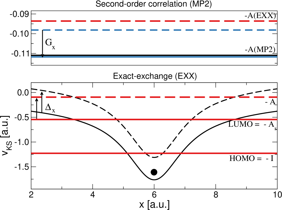
Figure 1: Lower panel: KS potential of a soft-Coulomb two-electron atom in the EXX approximation (black full and dashed curves). Horizontal lines indicates the KS HOMO and LUMO energy levels (red full) and the corrected affinity (red dashed). Upper panel: MP2 corrected affinity (blue dashed and full lines are without and with discontinuity, respectively). Black full line is the nonlocal MP2 result.

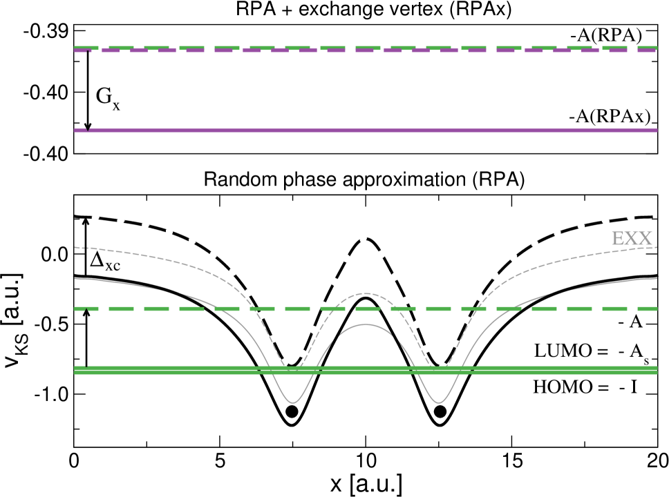
Figure 2: Lower panel: KS potential of a soft-Coulomb stretched H₂ molecule in the RPA approximation (black full and dashed curves). Horizontal lines indicates the KS HOMO and LUMO energy levels (green full) and the corrected affinity (green dashed). EXX approximation in the background (grey curves). Upper panel: RPAx corrected affinity (purple dashed and full lines are without and with discontinuity, respectively).

In Fig. 1 we present the results for a soft-Coulomb atomic system containing two electrons. The black dot signifies the location of the atom. In the lower panel we plot the EXX KS potential (full black line) obtained by imposing Eq. (4), which ensures the correct asymptotic limit of the potential. The dashed black line is the same potential but shifted by the EXX discontinuity ${\rm\Delta}_{\rm x}$ (Eq. (9)). This is the result one would get by evaluating the potential at $N=N_{0}^{+}$, as indicated to left with the arrows pointing upwards. The location of the KS HOMO (highest occupied molecular orbital) ($-I$) and the KS LUMO (lowest unoccupied molecular orbital) ($-A_{s}$) are indicated with full horizontal red lines. The red dashed horizontal line indicates the true affinity ($-A$) after correction with the discontinuity (Eq. (10)), also indicated by an arrow pointing upwards to the left.

The upper panel shows the correction to the affinity due to MP2 correlation. The red dashed A(EXX) line is the EXX affinity (a duplicate of the $-A$ line in the lower panel) and the blue dashed line is the correction due to the first term of Eq. (34). Keeping only this term corresponds to using Eq. (33) to calculate affinities. Including the discontinuity term (second term in Eq. (34), here called $G_{\rm x}$) further shifts the affinity (blue full horizontal line). Actually, we find that $G_{\rm x}$ corresponds to 75% of the total correction. The black full line in the same panel denoted A(MP2), is obtained by using the fully nonlocal vertex, i.e., by evaluating Eq. (31). We see that the black and blue full lines almost coincide. We can thus conclude that in order to reproduce the nonlocal MP2 approximation the discontinuity (i.e. the $G_{\rm x}$ term) of the EXX kernel is crucial.

IV.2 RPAx

We will now construct a more advanced self-energy that takes into account both screening and vertex corrections to all orders in the Coulomb interaction. In this way, we will consistently incorporate the EXX vertex in both the screened interaction (Eq. (15)) and in the self-energy (Eq. (14)). We call this self-energy RPAx

$${\rm\Sigma}^{\rm RPAx}=iG_{s}W_{\rm x}{\rm\Gamma}_{{\rm x}}.$$ (37)

This is the self-energy (although symmetrized) one obtains from the ACFD-formula including the EXX kernel (i.e. the RPAx energy) but by ignoring variations of $f_{\rm x}$ with respect to the density. hvb10 It can also be seen as the local approximation to the self-energy that includes vertex corrections at the time-dependent HF level. toulouse_prl

We applied this approximation to the stretched hydrogen molecule, for which we expect screening to be more important. In the lower panel of Fig. 2 we plot the KS potential at the RPA level (black full line). We also show the EXX potential in the background (grey thin line). The KS HOMO-LUMO gap is vanishing small but if we add the RPA discontinuity ${\rm\Delta}_{\rm xc}$ (obtained from Eq. (9) with the GW self-energy) the affinity shifts substantially. We also note that it is larger than the corresponding EXX correction, in agreement with the analysis in Ref. GWRPA, . Neither the HF nor the GWA is able to correctly describe the gap of stretched H₂ since it is a strongly correlated Mott-like system. GWRPA1 Including exchange effects in the vertex is not expected to qualitatively improve upon the GWA. Indeed, in the upper panel we present the results from the RPAx self-energy and we see that the correction is of the wrong sign. However, in this case, we see that the discontinuity is even more important to reproduce the nonlocality of the self-energy, accounting for almost the entire correction.

V Conclusions

In this work we have derived approximate self-energies based on local vertex corrections derived from XC kernels within the Klein MBPT formulation of TDDFT. These vertex corrections capture a dynamical discontinuity of the XC kernel, needed to accurately describe electron affinities. A numerical study on model molecular systems shows that the discontinuity of the local vertex corresponds to the largest correction to the GW affinity.

From the ACFD formula to the total energy we further show that an exact expression for the discontinuity of the XC potential can be written in terms of the XC kernel and its derivative. Although this work focused on the DD as a correction to the gap, a very important consequence of the discontinuity is to localise electrons in strongly correlated systems. The ability of an XC potential derived from the ACFD expression to do so will strongly rely on the discontinuous nature of the XC kernel.

VI Appendix

Here we give explicit expressions for the formulas in Sec. 4. The MP2 self-energy is composed of two terms. The second term in Eq. (31) is a first order screening correction so we denote it with a subscript $W_{1}$. In terms of orbitals and eigenvalues it is given by

$${\rm\Sigma}_{\rm W_{1}}({\bf r},{\bf r}^{\prime},\omega) = 2\sum_{kq}\varphi_{k}({\bf r})\int d{\bf r}_{1}v({\bf r},{\bf r}_{1})f^{*}_{q}({\bf r}_{1})$$ (38)

$$\!\!\!\!\!\!\!\!\!\!\!\!\!\!\!\!\!\!\!\!\!\!\!\!\!\!\!\times\varphi^{*}_{k}({\bf r}^{\prime})\int d{\bf r}_{1}v({\bf r}^{\prime},{\bf r}_{1})f_{q}({\bf r}_{1})$$

$$\!\!\!\!\!\!\!\!\!\!\!\!\!\!\!\!\!\!\!\!\!\!\!\!\!\!\!\times\left[\frac{n_{k}}{\omega-\varepsilon_{k}+Z_{q}-i\eta}+\frac{1-n_{k}}{\omega-\varepsilon_{k}-Z_{q}+i\eta}\right],$$

where $q$ is the particle-hole index, $f_{q}$ is the ’bare’ excitation function given by a product of occupied and unoccupied KS orbitals, and $Z_{q}$ is the corresponding eigenvalue difference. The first ’vertex’ term is instead given by

$${\rm\Sigma}_{\rm{\rm\Gamma}_{\rm HF}^{1}}({\bf r},{\bf r}^{\prime},\omega) = \sum_{ksp}\varphi^{*}_{k}({\bf r})\int d{\bf r}_{1}v({\bf r},{\bf r}_{1})\varphi_{s}({\bf r}_{1})\varphi_{p}({\bf r}_{1})$$ (39)

$$\!\!\!\!\!\!\!\!\!\!\!\!\!\!\!\!\!\!\!\!\!\!\!\!\!\!\!\!\!\!\!\!\!\!\!\!\!\!\!\!\!\!\!\times\,\,\varphi_{s}({\bf r}^{\prime})\int d{\bf r}_{1}v({\bf r}^{\prime},{\bf r}_{1})\varphi_{k}({\bf r}_{1})\varphi^{*}_{p}({\bf r}_{1})\times(-1)$$

$$\!\!\!\!\!\!\!\!\!\!\!\!\!\!\!\!\!\!\!\!\!\!\!\!\!\!\!\!\!\!\!\!\!\!\!\!\!\!\!\!\!\!\!\times\left[\frac{n_{k}n_{s}(1-n_{p})}{\omega-\varepsilon_{s}+\varepsilon_{p}-\varepsilon_{k}-i\eta}+\frac{(1-n_{k})n_{p}(1-n_{s})}{\omega-\varepsilon_{s}+\varepsilon_{p}-\varepsilon_{k}+i\eta}\right].$$

The sum of the terms (Eq. (38) and Eq. (39)) constitute the MP2 self-energy. The local MP2 self-energy also contains the term in Eq. (38) and in addition two local terms, one containing $f_{\rm x}$ and one its discontinuity $g_{\rm x}$. For a two-electron system the $f_{\rm x}$-term is just minus one half of Eq. (38). The second term is generated from Eq. (13) yielding

$$ig_{\rm x}\chi_{s}vG_{s} = \sum_{k,p\neq L}\varphi_{k}({\bf r}^{\prime})\int\!d{\bf r}_{1}\,v_{\rm x}({\bf r}_{1})\varphi_{p}({\bf r}_{1})\varphi^{*}_{L}({\bf r}_{1})$$ (40)

$$\!\!\!\!\!\!\!\!\!\!\!\!\!\!\!\!\!\!\!\!\!\!\!\!\!\!\!\times\varphi^{*}_{k}({\bf r})\int\!d{\bf r}_{1}\,v({\bf r},{\bf r}_{1})\varphi_{L}({\bf r}_{1})\varphi^{*}_{p}({\bf r}_{1})$$

$$\!\!\!\!\!\!\!\!\!\!\!\!\!\!\!\!\!\!\!\!\!\!\!\!\!\!\!\times\left[\frac{n_{k}}{\omega+\varepsilon_{L}-\varepsilon_{p}-\varepsilon_{k}-i\eta}+\frac{1-n_{k}}{\omega-\varepsilon_{L}+\varepsilon_{p}-\varepsilon_{k}+i\eta}\right]$$

$$\!\!\!\!\!\!\!\!\!\!\!\!\!\!\!\!\!\!\!\!\!\!\!\!\!\!\!+\sum_{s,k,p\neq L}\varphi_{k}({\bf r}^{\prime})n_{s}\int\!d{\bf r}_{1}d{\bf r}_{2}\varphi_{s}({\bf r}_{1})\varphi^{*}_{s}({\bf r}_{2})\,v({\bf r}_{1},{\bf r}_{2})\varphi_{p}({\bf r}_{1})\varphi^{*}_{L}({\bf r}_{2})$$

$$\!\!\!\!\!\!\!\!\!\!\!\!\!\!\!\!\!\!\!\!\!\!\!\!\!\!\!\times\varphi^{*}_{k}({\bf r})\int\!d{\bf r}_{1}\,v({\bf r},{\bf r}_{1})\varphi_{L}({\bf r}_{1})\varphi^{*}_{p}({\bf r}_{1})$$

$$\!\!\!\!\!\!\!\!\!\!\!\!\!\!\!\!\!\!\!\!\!\!\!\!\!\!\!\times\left[\frac{n_{k}}{\omega+\varepsilon_{L}-\varepsilon_{p}-\varepsilon_{k}-i\eta}+\frac{1-n_{k}}{\omega-\varepsilon_{L}+\varepsilon_{p}-\varepsilon_{k}+i\eta}\right]$$

$$\!\!\!\!\!\!\!\!\!\!\!\!\!\!\!\!\!\!\!\!\!\!\!\!\!\!\!+\sum_{kq}\varphi_{k}({\bf r})\int d{\bf r}_{1}v({\bf r},{\bf r}_{1})f^{*}_{q}({\bf r}_{1})$$

$$\!\!\!\!\!\!\!\!\!\!\!\!\!\!\!\!\!\!\!\!\!\!\!\!\!\!\!\times\varphi^{*}_{k}({\bf r}^{\prime})\int d{\bf r}_{1}d{\bf r}_{2}|\varphi_{L}({\bf r}_{2})|^{2}v({\bf r}_{2},{\bf r}_{1})f_{q}({\bf r}_{1})$$

$$\!\!\!\!\!\!\!\!\!\!\!\!\!\!\!\!\!\!\!\!\!\!\!\!\!\!\!\times\left[\frac{n_{k}}{\omega-\varepsilon_{k}+Z_{q}-i\eta}+\frac{1-n_{k}}{\omega-\varepsilon_{k}-Z_{q}+i\eta}\right]$$

$$\!\!\!\!\!\!\!\!\!\!\!\!\!\!\!\!\!\!\!\!\!\!\!\!\!\!\!+\sum_{kq}\varphi_{k}({\bf r})\int d{\bf r}_{1}v({\bf r},{\bf r}_{1})\varphi_{s}({\bf r}_{1})\varphi^{*}_{p}({\bf r}_{1})$$

$$\!\!\!\!\!\!\!\!\!\!\!\!\!\!\!\!\!\!\!\!\!\!\!\!\!\!\!\times\varphi^{*}_{k}({\bf r}^{\prime})\int d{\bf r}_{1}d{\bf r}_{2}\varphi^{*}_{L}({\bf r}_{1})\varphi_{L}({\bf r}_{2})v({\bf r}_{2},{\bf r}_{1})\varphi^{*}_{s}({\bf r}_{1})\varphi_{p}({\bf r}_{2})$$

$$\!\!\!\!\!\!\!\!\!\!\!\!\!\!\!\!\!\!\!\!\!\!\!\!\!\!\!\times\left[\frac{n_{k}n_{s}(1-n_{p})}{\omega-\varepsilon_{k}+\varepsilon_{p}-\varepsilon_{s}-i\eta}+\frac{(1-n_{k})n_{s}(1-n_{p})}{\omega-\varepsilon_{k}-\varepsilon_{p}-\varepsilon_{s}+i\eta}\right]$$

References

- (1) W. Kohn, L.J. Sham, Phys. Rev. 140, A1133 (1965)
- (2) E. Runge, E.K.U. Gross, Phys. Rev. Lett. 52, 997 (1984)
- (3) C.O. Almbladh, U. von Barth, in Density Functional Methods in Physics, Vol. 123 of NATO Advanced Study Institute Series B: Physics, edited by R.M. Dreizler, J. da Providencia (Plenum, New York, 1985)
- (4) J.P. Perdew, in Density Functional Methods in Physics, Vol. 123 of NATO Advanced Study Institute Series B: Physics, edited by R.M. Dreizler, J. da Providencia (Plenum, New York, 1985)
- (5) O.V. Gritsenko, E.J. Baerends, Phys. Rev. A 54, 1957 (1996)
- (6) N. Helbig, I.V. Tokatly, A. Rubio, The Journal of Chemical Physics 131, 224105 (2009)
- (7) P. Elliott, J.I. Fuks, A. Rubio, N.T. Maitra, Phys. Rev. Lett. 109, 266404 (2012)
- (8) M.J.P. Hodgson, E. Kraisler, A. Schild, E.K.U. Gross, The Journal of Physical Chemistry Letters 8, 5974 (2017)
- (9) J.P. Perdew, R.G. Parr, M. Levy, J.L. Balduz, Phys. Rev. Lett. 49, 1691 (1982)
- (10) J.B. Krieger, Y. Li, G.J. Iafrate, Phys. Rev. A 45, 101 (1992)
- (11) M. Hellgren, E.K.U. Gross, Phys. Rev. A 88, 052507 (2013)
- (12) A.D. Becke, The Journal of Chemical Physics 98, 1372 (1993)
- (13) B. Himmetoglu, A. Floris, S. de Gironcoli, M. Cococcioni, International Journal of Quantum Chemistry 114, 14 (2014)
- (14) M. Hellgren, D.R. Rohr, E.K.U. Gross, J. Chem. Phys. 136, 034106 (2012)
- (15) F. Caruso, D.R. Rohr, M. Hellgren, X. Ren, P. Rinke, A. Rubio, M. Scheffler, Phys. Rev. Lett. 110, 146403 (2013)
- (16) M. Hellgren, F. Caruso, D.R. Rohr, X. Ren, A. Rubio, M. Scheffler, P. Rinke, Phys. Rev. B 91, 165110 (2015)
- (17) N. Colonna, M. Hellgren, S. de Gironcoli, Phys. Rev. B 93, 195108 (2016)
- (18) A. Grüneis, M. Marsman, J. Harl, L. Schimka, G. Kresse, The Journal of Chemical Physics 131, 154115 (2009)
- (19) X. Ren, P. Rinke, G.E. Scuseria, M. Scheffler, Phys. Rev. B 88, 035120 (2013)
- (20) X. Ren, N. Marom, F. Caruso, M. Scheffler, P. Rinke, Phys. Rev. B 92, 081104 (2015)
- (21) J. Toulouse, I.C. Gerber, G. Jansen, A. Savin, J.G. Ángyán, Phys. Rev. Lett. 102, 096404 (2009)
- (22) J.E. Bates, F. Furche, The Journal of Chemical Physics 139, 171103 (2013)
- (23) M. Hellgren, U. von Barth, J. Chem. Phys. 132, 044101 (2010)
- (24) A. Heßelmann, A. Görling, Molecular Physics 108, 359 (2010)
- (25) N. Colonna, M. Hellgren, S. de Gironcoli, Phys. Rev. B 90, 125150 (2014)
- (26) P. Bleiziffer, M. Krug, A. Görling, The Journal of Chemical Physics 142, 244108 (2015)
- (27) R. Del Sole, R. Reining, R.W. Godby, Phys. Rev. B 49, 8024 (1994)
- (28) E.K.U. Gross, W. Kohn, Phys. Rev. Lett. 55, 2850 (1985)
- (29) F. Bruneval, F. Sottile, V. Olevano, R. Del Sole, L. Reining, Phys. Rev. Lett. 94, 186402 (2005)
- (30) M. Petersilka, U.J. Gossmann, E.K.U. Gross, Phys. Rev. Lett. 76, 1212 (1996)
- (31) M. Hellgren, E.K.U. Gross, Phys. Rev. A 85, 022514 (2012)
- (32) M. Hellgren, E.K.U. Gross, J. Chem. Phys. 136, 114102 (2012)
- (33) P. Romaniello, S. Guyot, L. Reining, J. Chem. Phys. 131, 154111 (2009)
- (34) E. Sagvolden, J.P. Perdew, Phys. Rev. A 77, 012517 (2008)
- (35) P. Mori-Sánchez, A.J. Cohen, W. Yang, Phys. Rev. Lett. 102, 066403 (2009)
- (36) A. Mirtschink, M. Seidl, P. Gori-Giorgi, Phys. Rev. Lett. 111, 126402 (2013)
- (37) S. Kurth, G. Stefanucci, E. Khosravi, C. Verdozzi, E.K.U. Gross, Phys. Rev. Lett. 104, 236801 (2010)
- (38) M. Lein, S. Kümmel, Phys. Rev. Lett. 94, 143003 (2005)
- (39) G. Stefanucci, S. Kurth, Phys. Rev. Lett. 107, 216401 (2011)
- (40) J.P. Bergfield, Z.F. Liu, K. Burke, C.A. Stafford, Phys. Rev. Lett. 108, 066801 (2012)
- (41) A. Dreuw, M. Head-Gordon, Journal of the American Chemical Society 126, 4007 (2004)
- (42) C.O. Almbladh, U. von Barth, Phys. Rev. B 31, 3231 (1985)
- (43) O. Gunnarsson, K. Schönhammer, Phys. Rev. Lett. 56, 1968 (1986)
- (44) M. Grüning, A. Marini, A. Rubio, Phys. Rev. B 74, 161103 (2006)
- (45) M.J. Allen, D.J. Tozer, Molecular Physics 100, 433 (2002)
- (46) T. Stein, H. Eisenberg, L. Kronik, R. Baer, Phys. Rev. Lett. 105, 266802 (2010)
- (47) A.J. Cohen, P. Mori-Sánchez, W. Yang, Science 321, 792 (2008)
- (48) Z.J. Ying, V. Brosco, J. Lorenzana, Phys. Rev. B 89, 205130 (2014)
- (49) K. Fukui, T. Yonezawa, H. Shingu, The Journal of Chemical Physics 20, 722 (1952)
- (50) K. Fukui, Science 218, 747 (1982)
- (51) F.G. Eich, M. Hellgren, J. Chem. Phys. 141, 224107 (2014)
- (52) U. von Barth, N.E. Dahlen, R. van Leeuwen, G. Stefanucci, Phys. Rev. B 72, 235109 (2005)
- (53) A. Klein, Phys. Rev. 121, 950 (1961)
- (54) L.J. Sham, Phys. Rev. B 32, 3876 (1985)
- (55) L.J. Sham, M. Schlüter, Phys. Rev. B 32, 3883 (1985)
- (56) R.W. Godby, M. Schlüter, L.J. Sham, Phys. Rev. B 36, 6497 (1987)
- (57) R.W. Godby, M. Schlüter, L.J. Sham, Phys. Rev. B 37, 10159 (1988)
- (58) M.E. Casida, Phys. Rev. A 51, 2005 (1995)
- (59) L. Hedin, Phys. Rev. 139, A796 (1965)
- (60) F. Aryasetiawan, O. Gunnarsson, Rep Prog Phys 61, 237 (1998)
- (61) L. Reining, WIREs Comput Mol Sci p. e1344 (2017)
- (62) G. Baym, L. Kadanoff, Phys. Rev. 124, 286 (1961)
- (63) G. Baym, Phys. Rev. 127, 1391 (1962)
- (64) Y.M. Niquet, M. Fuchs, X. Gonze, Phys. Rev. A 68, 032507 (2003)
- (65) J.B. Krieger, Y. Li, G.J. Iafrate, Phys. Rev. A 45, 101 (1992)
- (66) Y.H. Kim, A. Görling, Phys. Rev. Lett. 89, 096402 (2002)
- (67) H. Bachau, E. Cormier, P. Decleva, J.E. Hansen, F. Martin, Rep. Prog. Phys. 64, 1815 (2001)
- (68) M. Hellgren, U. von Barth, Phys. Rev. B 76, 075107 (2007)
- (69) H. Jiang, E. Engel, J. Chem. Phys. 123, 224102 (2005)