A Distributed Algorithm for Finding Hamiltonian Cycles in Random Graphs in $O(\log n)$ Time

Abstract

It is known for some time that a random graph $G(n,p)$ contains w.h.p. a Hamiltonian cycle if $p$ is larger than the critical value $p_{crit}=(\log n+\log\log n+\omega_{n})/n$. The determination of a concrete Hamiltonian cycle is even for values much larger than $p_{crit}$ a nontrivial task. In this paper we consider random graphs $G(n,p)$ with $p$ in $\tilde{\Omega}(1/\sqrt{n})$, where $\tilde{\Omega}$ hides poly-logarithmic factors in $n$. For this range of $p$ we present a distributed algorithm ${\cal A}_{\mathsf{HC}}$ that finds w.h.p. a Hamiltonian cycle in $O(\log n)$ rounds. The algorithm works in the synchronous model and uses messages of size $O(\log n)$ and $O(\log n)$ memory per node.

1 Introduction

Surprisingly few distributed algorithms have been designed and analyzed for random graphs. To the best of our knowledge the only work dedicated to the analysis of distributed algorithms for random graphs is [17, 16, 5]. This is rather surprising considering the profound knowledge about the structure of random graphs available since decades [3, 10]. While algorithms designed for general graphs obviously can be used for random graphs the specific structure of random graphs often allows to prove asymptotic bounds that are far better. In the classical Erdős and Rényi model for random graphs a graph $G(n,p)$ is an undirected graph with $n$ nodes where each edge independently exists with probability $p$ [7]. The complexity of algorithms for random graphs often depends on $p$, e.g., Krzywdziński et al. [16] proposed a distributed algorithm that finds w.h.p. a coloring of $G(n,p)$ with $18np$ colors in $O(\ln\ln p^{-1})$ rounds.

In this work we focus on finding Hamiltonian cycles in random graphs. The decision problem, whether a graph contains a Hamiltonian cycle, is NP-complete. It is a non-local graph problem, i.e., it is required to always consider the entire graph in order to solve the problem. It is impossible to solve it in the local neighborhoods. For this reason there is almost no work on distributed algorithms for finding Hamiltonian cycles in general graphs. On the other hand it is well known that $G(n,p)$ contains w.h.p. a Hamiltonian cycle, provided $p\geq p_{crit}=(\log n+\log\log n+\omega(n))/n$, where $\omega(n)$ satisfies $\lim_{n\to\infty}\omega(n)=\infty$ [3, Th. 8.9]. There is a large body of work on sequential algorithms for computing w.h.p. a Hamiltonian cycle in a random graph (e.g. [21, 1, 23, 4, 25]).

We are only aware of two distributed algorithms for computing Hamiltonian cycles in random graphs. The algorithm by Levy et al. [17] outputs w.h.p. a Hamiltonian cycle provided $p=\omega(\sqrt{\log n}/n^{1/4})$. This algorithm works in synchronous distributed systems, terminates in linear worst-case number of rounds, requires $O(n^{3/4+\epsilon})$ rounds on expectation, and uses $O(n)$ space per node. The algorithm of Chatterjee et al. [5] works for $p\geq c\log n/n^{\delta}$ ($0<\delta\leq 1$) and has a run time of $\tilde{O}(n^{\delta})$.

The search for a distributed algorithm for a Hamiltonian cycle is motivated by the usage of virtual rings for routing in wireless networks [19, 26]. A virtual ring is a directed closed path involving each node of the graph, possibly several times. Virtual rings enable routing with constant space routing tables, messages are simply forwarded along the ring. The downside is that they may incur a linear path stretch. To attenuate this, distributed algorithms for finding short virtual rings have been proposed [12, 26]. Hamiltonian cycles are the shortest possible virtual rings and therefore of great interest. Short virtual rings are also of interest for all token circulation techniques as discussed in [8]. Kim et al. discuss the application of random Hamiltonian cycles for peer-to-peer streaming [13]. Rabbat et al. present distributed optimization algorithms for in-network data processing, aimed at reducing the amount of energy and bandwidth used for communication based on Hamiltonian cycles [22], see also [24].

This paper uses the synchronous $\mathcal{CONGEST}$ model, i.e., each message contains at most $O(\log n)$ bits. Furthermore, each node has only $O(\log n)$ bits of local memory. Without these two assumptions there is a very simple solution provided the nodes have unique identifiers. First a BFS-tree rooted in a node $v_{0}$ is constructed. Then the adjacency list of each node is convergecasted to $v_{0}$ which applies a sequential algorithm to compute w.h.p. a Hamiltonian path (see Sec. 1.1). The result is broadcasted into the graph and thus each node knows its neighbor in the Hamiltonian cycle. This can be achieved in $O(diam(G))$ rounds. Note that if $p=\omega_{n}\log n/n$ then w.h.p. $diam(G(n,p))=O\left(\frac{\log n}{\log np}\right)$ [6, 10]. In particular for $p$ in $\tilde{\Omega}(1/\sqrt{n})$ w.h.p. the diameter of $G(n,p)$ is constant [2].

For the stated restrictions on message size and local storage we propose an algorithm that terminates in a logarithmic number of rounds, this is a significant improvement over previous work [17, 5]. Our contribution is the distributed algorithm ${\cal A}_{\mathsf{HC}}$, its properties can be summarized as follows.

Theorem 1.

Let $G(n,p)$ with $p\geq(\log n)^{3/2}/\sqrt{n}$ be a random graph. Algorithm ${\cal A}_{\mathsf{HC}}$ computes in the synchronous model w.h.p. a Hamiltonian cycle for $G$ using messages of size $O(\log n)$. ${\cal A}_{\mathsf{HC}}$ terminates in $O(\log n)$ rounds and uses $O(\log n)$ memory per node.

1.1 Related Work

Pósa showed already in 1976 that almost all random graphs with $cn\log n$ edges possess a Hamiltonian cycle [21]. Later Komlós et al. determined the precise threshold $p_{crit}$ for the existence of a Hamiltonian cycle in a random graph [14]. A sequential deterministic algorithm that works w.h.p. at this threshold requiring $O(n^{3+o(1)})$ time is due to Bollobás et al. [4]. For larger values of $p$ or restrictions on the minimal node degree, more efficient algorithms are known [1, 11]. The algorithm of Thomason finds a Hamiltonian path or shows that no such path exists provided $p\geq 12n^{-1/3}$ [25].

The above cited algorithms were all designed for the sequential computing model. Some exact algorithms for finding Hamiltonian cycles in $G(n,p)$ on parallel computers have been proposed [9]. The first operates in the EREW-PRAM model and uses $O(n\log n)$ processors and $O(\log^{2}n)$ time, while the second one uses $O(n\log^{2}n)$ processors and $O((\log\log n)^{2})$ time in the P-RAM model. MacKenzie and Stout proposed an algorithm for CRCW-PRAM machines that operates in $O(\log^{\ast}n)$ expected time and requires $n/\log^{\ast}n$ processors [18]. Apart from the above mentioned work [17, 5] we are not aware of any other distributed algorithm for this problem.

There are several approaches to construct a Hamiltonian cycle. The approach used by Levy et al. at least goes back to the work of MacKenzie and Stout [18]. They initially construct a small cycle with $\Theta(\sqrt{n})$ nodes. As many as possible of the remaining nodes are assorted in parallel into $\sqrt{n}$ vertex-disjoint paths. During the final phase, each path and each non-covered vertex is patched into the initial cycle.

The second approach is used in the proofs to establish the critical value $p_{crit}$ (e.g., [21, 15]) and all derived sequential algorithms (e.g., [4]). Initially a preferably long path is constructed, e.g., using a depth first search algorithm [11]. This path is extended as long as the node at the head of the path has a neighbor that is not yet on the path. Then the path is rotated until it can be extended again. A rotation of the path cuts off a subpath beginning at the head, reverses the order of the subpath’s nodes, and reattaches the subpath again. The procedure stops when no sequence of rotations leads to an extendable path. The algorithm in [5] follows this approach.

2 Computational Model and Assumptions

This work employs the synchronous $\mathcal{CONGEST}$ model of the distributed message passing model [20], i.e., each message contains at most $O(\log n)$ bits. Furthermore, each node has only $O(\log n)$ bits of local memory. The communication network is represented by an undirected graph $G=(V,E)$, where $V$ is a set of $n$ processors (nodes) and $E$ represents the set of $m$ bidirectional communication links (edges) between them. Each node carries a unique identifier. Communication between nodes is performed in synchronous rounds using messages exchanged over the links. Upon reception of a message, a node performs local computations and possibly sends messages to its neighbors. These operations are assumed to take negligible time.

The prerequisite of Algorithm ${\cal A}_{\mathsf{HC}}$ is a distinguished node $v_{0}$ which is the starting point of the Hamiltonian cycle and acts as a coordinator in the final phases of ${\cal A}_{\mathsf{HC}}$. The results proved in this work hold with high probability (w.h.p.) which means with probability tending to $1$ as $n\rightarrow\infty$. The probabilities $p$ considered in this paper always depended on $n$, e.g., $p\geq(\log n)^{3/2}/\sqrt{n}$, and we always assume that $\lim_{n\rightarrow\infty}p=0$.

3 Informal Description of Algorithm ${\cal A}_{\mathsf{HC}}$

Algorithm ${\cal A}_{\mathsf{HC}}$ operates in sequential phases, each of them succeeds w.h.p. The first two phases last $O(\log n)$ rounds. Each subsequent phase requires a constant number of rounds only. Phase 0 lasts $3(3\log n-1)$ rounds and constructs a path $P$ of length $3\log n$ starting in $v_{0}$. In the next $3\log n$ rounds Phase 1 closes $P$ into a cycle $C$ of length at most $4\log n$. The following $16\log(n)$ phases are called the middle phases. In each of those phases the number of nodes in $C$ is increased. The increase is by a constant factor until $C$ has $n/7$ nodes. Afterwards, the increase declines roughly linearly until $C$ has $n-3\log n$ nodes. In each middle phase the algorithm tries to concurrently integrate as many nodes into $C$ as possible. This is achieved by replacing edges ($v,w)$ of $C$ by two edges $(v,x)$ and $(x,w)$, where $x$ is a node outside of $C$. At the end of the middle phases w.h.p. $C$ has more than $n-3\log n$ nodes.

The integration of the remaining $3\log n$ nodes requires a more sophisticated algorithm. This is done in the final phases. The idea is to remove two edges – not necessarily adjacent – from $C$ and insert three new edges. This requires to reverse the edges of a particular segment of $C$ of arbitrary length. Thus, this is no longer a local operation. Furthermore, segments may overlap and hence, the integration of several nodes can only be performed sequentially. Thus, this task requires coordination. Node $v_{0}$ takes over the role of a coordinator.

At the beginning of each final phase all nodes outside $C$ that can be integrated report this to $v_{0}$, which in turn selects one of these nodes to perform this step. For this purpose a tree routing structure is set up, so that each node can reach $v_{0}$ w.h.p. in $3$ hops. In order for the nodes of the segment to perform the reordering concurrently, the nodes of $C$ are numbered in an increasing order (not necessarily consecutively) beginning with $v_{0}$. The assignment of numbers is embedded into the preceding phases with no additional overhead. The numbering is also maintained in the final $3\log n$ integration steps. In order to accomplish the integration in a constant number of rounds – i.e., independent of the length of the segment – node $v_{0}$ floods the numbers of the terminal nodes of the segment to be reversed into the network. Upon receiving this information, each node can determine if it belongs to the segment to be reversed and can recompute its number to maintain the ordering. Note that this routing structure requires only $O(\log n)$ memory per node. Each of the $3\log n$ final phases lasts a constant number of rounds.

Algorithm ${\cal A}_{\mathsf{HC}}$ stops when either $C$ is a Hamiltonian cycle or no more nodes can be integrated into $C$. The first event occurs w.h.p.

4 Formal Description

Algorithm ${\cal A}_{\mathsf{HC}}$ operates in synchronous rounds. By counting the rounds a node is always aware in which round and therefore also in which phase it is. Each phase lasts a known fixed number of rounds. If the work is completed earlier, the network is idle for the remaining rounds. This requires each node to know $n$. Algorithm ${\cal A}_{\mathsf{HC}}$ gradually builds an oriented cycle $C$ starting with node $v_{0}$. The cycle is maintained as a doubly linked list to support insertions. The orientation of $C$ is administered with the help of variable $next$ – initially $null$ – which stores the identifier of the next node on the cycle in clockwise order. Also, $v.next=null$ indicates that $v$ is not yet on the cycle. In the following each phase is described in detail.

4.1 Pre-processing

The algorithm is started by node $v_{0}$ which executes algorithm Flood [20] to construct a BFS tree. By Lemma 16 the diameter of $G$ is w.h.p. at most 3. Thus, in $3$ rounds a BFS tree rooted in $v_{0}$ is constructed (Lemma 5.3.1, [20]). After a further $6$ rounds each node is aware of $n$ the number of nodes in the network. This allows to run each phase for the stated number of rounds.

4.2 Phase 0

In phase 0 an oriented path $P$ starting in $v_{0}$ of length $3\log n$ is constructed. Phase 0 lasts $3(3\log n-1)$ rounds. Initially $P=\{v_{0}\}$ and $v_{0}.next=v_{0}$. The following steps are repeated $3\log n-1$ times.

1. The final node $v$ of $P$ sends an invitation message to all neighbors. All neighbors not on $P$ (i.e., nodes with $next=null$) respond to $v$.

2. If $v$ does not receive any response the algorithm halts. Otherwise $v$ randomly selects among the nodes that have responded a node $w$, sets $v.next:=w$, informs $w$ that it is the new final node, and instructs $w$ to continue with phase 0. This message includes the id of node $v_{0}$, i.e., at any point in time all nodes of $P$ know $v_{0}$.

4.3 Phase 1

In phase 1 the path $P$ is extended into an oriented cycle $C$ of length at most $4\log n$. The following steps are repeated at most $\log n$ times. Phase 1 lasts $3\log n$ rounds.

1. The final node $v$ of $P$ sends an invitation message to all neighbors, the message contains the id of node $v_{0}$. All neighbors not on $P$ respond to $v$. The response includes the information whether the recipient is connected to $v_{0}$.

2. If $v$ does not receive any response the algorithm halts. If at least one responding node is connected to $v_{0}$, then $v$ randomly selects such a node $w$, sets $v.next=w$, and informs $w$ to close the cycle $C$, i.e., to set $w.next=v_{0}$. Otherwise $v$ randomly selects a responding node $w$ to extend $P$ as in phase 0 and instructs $w$ to repeat phase 1.

3. If after $\log n$ repetitions $P$ is not a cycle then the algorithm halts otherwise the middle phases start.

4.4 Middle Phases

While in the first two phases actions were executed sequentially, in the middle phases many nodes are integrated concurrently. In each of the subsequent phases the following steps are performed (see Fig. 1 for an example). Each of the $16\log n$ middle phases is performed in three rounds.

1. Each node $w$ on $C$ broadcasts its own id and the id of its predecessor on $C$ using message $I_{1}$.

2. If a node $v$ outside $C$ receives a message $I_{1}$ from a node $w$ such that the predecessor of $w$ on $C$ is a neighbor of $v$, it inserts $w$ into the set $C_{v}$.

3. Each node $v$ outside $C$ with $C_{v}\not=\emptyset$ randomly selects a node $w$ from $C_{v}$ and sends an invitation message $I_{2}$ to the predecessor of $w$ on $C$.

4. Each node $w\in C$ that received an invitation $I_{2}$ randomly selects a node $v$ from which it received an invitation, sets $w.next=v$, and informs $v$ with acceptance message $I_{3}$ to set its variable $next$ to the old successor $w^{\prime}$ of $w$. In other words the edge $(w,w^{\prime})$ is replaced by the edges $(w,v)$ and $(v,w^{\prime})$.

Individual extensions do not interfere with each other. Each node outside $C$ gets in the last round of a middle phase at most one request for extension and for each edge of $C$ at most one request is sent.

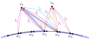
Figure 1: The integration of nodes during a middle phase: Nodes $w_{i}$ sent a message $I_{1}$ to all nodes outside $C$ (red arrows). Nodes $v_{1}$ and $v_{2}$ sent a message $I_{2}$ back to $w_{4}$; $v_{2}$ might have also selected $w_{4}$ and sent $I_{3}$ to $w_{5}$. Node $w_{4}$ selected $v_{1}$ and sent back message $I_{3}$. Edge $(w_{4},w_{3})$ is replaced by the edges $(w_{4},v_{1})$ and $(v_{1},w_{3})$. The extended cycle is depicted by the blue ribbon.

4.5 Final Phases

After the completion of the middle phases the cycle $C$ has w.h.p. at least $n-3\log n$ nodes. At that point the expected number of nodes $v\in V\setminus C$ that send an invitation $I_{2}$ becomes too low to complete the cycle. Therefore, the integration of the remaining nodes requires a more complex integration procedure as depicted in Fig. 2. The procedure of the final phases is as follows. Each node $v\in V\setminus C$ with identifier $id$ sends a message $I_{1}(id)$ to each of its neighbors. A node $w_{1}\in C$ that receives a message $I_{1}(id)$ sends a message $I_{2}(id)$ to its neighbor $w_{2}$ on $C$ in clockwise order. If $w_{2}$ also received a message $I_{1}(id)$ (with the same id), then nodes $w_{1},w_{2}$ and the initiating node $v$ with identifier $id$ form a triangle. Then $v$ can be directly integrated into $C$ as done in the middle phases. In this case $w_{1}$ asks $v$ to initiate the integration step.

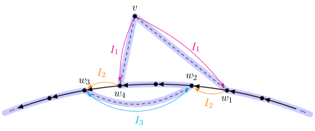
Figure 2: The integration of node $v$ into $C$ during the final phase. The thin red arrows indicate the flow of the messages $I_{1},I_{2}$, and $I_{3}$ initiated by $v$. The extended cycle is depicted by the blue ribbon. The edges $(w_{1},w_{2})$ and $(w_{4},w_{3})$ are replaced by the edges $(w_{1},v)$, $(v,w_{4})$, and $(w_{2},w_{3})$. The order of the edges between $w_{4}$ and $w_{2}$ is reversed.

Otherwise, if node $w_{2}$ did not receive a message $I_{1}(id)$, then it sends a message $I_{3}(id)$ to all neighbors that are on $C$. If a node $w_{3}$ on $C$ that receives this message $I_{3}(id)$ also received a message $I_{2}(id)$ from its predecessor $w_{4}$ on $C$, then node $v$ can be integrated into $C$ as shown in Fig. 2. This is achieved by replacing edges $(w_{1},w_{2})$ and $(w_{4},w_{3})$ from $C$ by edges $(w_{1},v)$, $(v,w_{4})$, and $(w_{2},w_{3})$. Also, the edges on the segment from $w_{2}$ to $w_{4}$ must be traversed in opposite order, note that the number of nodes between $w_{2}$ and $w_{4}$ is not bounded. A naive explicit reversing of the order of the edges on the middle segment may require more than $O(\log n)$ rounds. Thus, we propose a different approach.

Apart from the reversal of the edges in the middle segment this integration can be implemented within five rounds. Node $w_{3}$ informs $v$ about this integration possibility, this notification also includes the identifiers of nodes $w_{4}$ and $w_{2}$. Furthermore, the participating nodes $w_{4},w_{2}$ and $w_{1}$ are also informed. The approach to invert the middle segment in a constant number of rounds is explained below.

Unfortunately there is another issue. While each node outside $C$ can be integrated individually, these integration steps cannot be executed concurrently. A problem arises if the segments, which are inverted (e.g. from $w_{2}$ to $w_{4}$), overlap. This can result in two separate cycles as shown in Fig. 3. Even if the integration of the remaining nodes is performed sequentially, a problem appears if the reversal of the middle segment is not made explicit. In this case the nodes that receive an $I_{1}$ message may not have a consistent view with respect to the clockwise order of $C$.

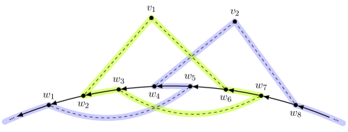
Figure 3: The depicted scenario shows that the integration of two nodes with overlapping segments cannot be performed concurrently as this would lead to two cycles (shown in green and blue). If $v_{2}$ would be integrated first, then $v_{1}$ can no longer be integrated, since the predecessor of $w_{6}$ is then $w_{5}$ which is not connected to $w_{3}$.

The solution to the problem of interfering concurrent integrations is to serialize all integration steps. For this purpose node $v_{0}$ acts as a coordinator. In each of the final phases each node $v$ outside $C$ first checks if can be integrated using the above described sequence of messages $I_{1}$ to $I_{3}$. If this is the case then $v$ randomly selects one of these possibilities and informs $v_{0}$. This message includes information about the four nodes on $C$ that characterize the integration (see below for details). Node $v_{0}$ selects among all offers a single node $v$ and informs it. Upon receiving the integration order, a node $v$ initialize the integration which is completed after fives rounds. Then the integration of the next node can start.

The solution for the second problem – the reversal of the segment – is based on an ascending numbering of the nodes. Such a numbering can easily be established in the first and middle phases. During phases 0 and 1 the nodes are numbered as follows: Node $v_{0}$ has number $0$. In clockwise order the nodes have numbers $n^{14},2n^{14},3n^{14},\ldots$, $\beta n^{14}$ for some integer constant $\beta\leq\lceil 4\log n\rceil$. Thus, the difference between two consecutive nodes is $n^{14}$. During the middle phases when a node $v$ is integrated into $C$ between two nodes with numbers $f<l$ the integrated node gets the number $\lceil(f+l)/2\rceil$. This is an integer strictly between $f$ and $l$ as long as $|f-l|\geq 2$. If a node is integrated between $v_{0}$ and the node with the highest number $y$, the new number is $y+\lceil(\beta+1)n/2\rceil$. It is straightforward to verify that all numbers are different and are ascending along the cycle beginning with $v_{0}$. The choice of the initial numbers guarantees that the difference of the numbers of two consecutive nodes is always at least $2$.

In case a node $v$ is integrated during the final phase it gets the number $\lceil(n_{1}+n_{2})/2\rceil$ as if it would be inserted between $w_{1}$ and $w_{2}$ with numbers $n_{1}$ and $n_{2}$ (see Fig. 2). The numbers of the nodes between $w_{2}$ and $w_{4}$ need to be updated such that overall the numbers are ascending. When a node can be integrated it includes in the notification message to $v_{0}$ the numbers of the end nodes of the segment that would be reversed if this node is integrated, i.e., the numbers of $w_{2}$ and $w_{4}$ (referred to as $f$ and $l$ in the following). Afterwards, when $v_{0}$ informs the selected node it distributes a message to all nodes in the network that also includes the numbers $f$ and $l$. A node receiving this message checks if its own number $x$ is between $f$ and $l$. In this case it changes its number to $f+l-x$. Thus, the numbers of the nodes in the segment are reflected on the mid point of the segment (see Fig. 4). Each node that changes its number also updates it next pointer to the other neighbor on $C$. Also nodes $v,w_{1}$, and $w_{2}$ update their next pointer.

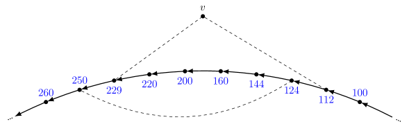
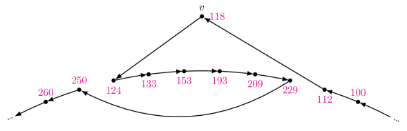
Figure 4: Node $v$ is to be integrated into $C$. The nodes $w_{1}$ and $w_{2}$ have the numbers $f=124$ and $l=229$. Node $v$ will receive number $\lceil(112+124)/2\rceil=118$. Upon receiving the message form node $v_{0}$, nodes with a number between 124 and 229 change their numbers. The left sides shows the old numbers and the right side the new numbers.

This procedure results in a cycle including $v$ with a numbering that is consistent with the orientation. Thus, when the integration phase of the next node starts, cycle $C$ is in a consistent state. To carry out this phase a short route from each node to $v_{0}$ and vice versa is needed. This is provided by the BFS tree constructed in the pre-processing phase: Each node reaches $v_{0}$ in at most 3 hops. Thus, each final phase lasts 11 rounds.

5 Analysis of Algorithm ${\cal A}_{\mathsf{HC}}$

This section proves the correctness and analyzes the complexity of the individual phases and proves the main theorem. First, we prove that ${\cal A}_{\mathsf{HC}}$ produces the numbering that guarantees that the final phases work correctly. Afterwards the individual phases are analyzed. Some of the results are proved for values of $p$ less than $(\log n)^{3/2}/\sqrt{n}$ to make them more general.

Lemma 1.

At the end of each phase each node has a different number and the numbers are ascending beginning with number $0$ for node $v_{0}$ in clockwise order.

Proof.

After phase 1 starting with node $v_{0}$ the nodes have the numbers $n^{14},2n^{14},3n^{14},\ldots$, $\beta n^{14}$, i.e., the difference between the numbers of two neighboring nodes on $C$ is $n^{14}$. A node $v$ that is inserted between two nodes with integral numbers $x$ and $y$ in middle phase gets the number $\lceil(x+y)/2\rceil$. Let $x<y$. If $x+y$ is even then $|x-\lceil(x+y)/2\rceil|=|y-\lceil(x+y)/2\rceil|=d/2$. If $x+y$ is odd then $|x-\lceil(x+y)/2\rceil|=(d+1)/2$ and $|y-\lceil(x+y)/2\rceil|=(d-1)/2$. This yields that the distance $d$ between two consecutive numbers is approximately at most cut in half, i.e., the smaller part is at least $(d-1)/2$. After $i$ middle phases the distance between to numbers is at least

$$\frac{d}{2^{i}}-\left(1-\frac{1}{2^{i}}\right)$$ (1)

Since there are $16\log n$ middle phases the distance between two numbers is $n^{14}/2^{16\log n}-(1-1/2^{16\log n})>2^{(3\log n)+1}$. This implies that after the middle phases the numbering of the nodes satisfies the stated condition.

Let $v$ be a node that is inserted in a final phase into $C$. Assume that the smallest distance between the numbers of two consecutive nodes on $C$ is at least $2$. Consider Fig. 2 for reference. Let $f$ (resp. $l$) the number of $w_{1}$ (resp. $w_{3}$) at the beginning of the corresponding final phase. Denote the nodes between $w_{2}$ and $w_{4}$ by $w^{\prime}_{1},\ldots,w^{\prime}_{k}$ with $w_{2}=w^{\prime}_{1}$ and $w_{4}=w^{\prime}_{k}$. Furthermore, let $n^{\prime}_{1},\dots,n^{\prime}_{k}$ be the numbers of these nodes. Thus,

$$f<n^{\prime}_{1}<\ldots<n^{\prime}_{k}<l$$

The order of these nodes on $C$ at the end of the phase will be $w_{1},v,w^{\prime}_{k},\ldots,w^{\prime}_{1},w_{3}$. Denote by $n_{i}$ the new number of node $w^{\prime}_{i}$, i.e., $n_{i}=n^{\prime}_{1}+n^{\prime}_{k}-n^{\prime}_{i}$. Thus, we need to prove

$$f<\lceil(f+n^{\prime}_{1})/2\rceil<n_{k}<n_{k-1}<\ldots<n_{1}<l$$

Since $n^{\prime}_{1}>f+1$ it follows $f<\lceil(f+n^{\prime}_{1})/2\rceil$ and since $n_{k}=n^{\prime}_{1}+n^{\prime}_{k}-n^{\prime}_{k}=n^{\prime}_{1}>f+1$ it follows $\lceil(f+n^{\prime}_{1})/2\rceil<n_{k}$. Furthermore, $n^{\prime}_{i}<n^{\prime}_{i+1}$ implies $n_{i+1}=n^{\prime}_{1}+n^{\prime}_{k}-n^{\prime}_{i+1}<n^{\prime}_{1}+n^{\prime}_{k}-n^{\prime}_{i}=n_{i}$. Finally, $n_{1}=n^{\prime}_{1}+n^{\prime}_{k}-n^{\prime}_{1}=n^{\prime}_{k}<l$.

As shown above at the end of the middle phases $d>2^{(3\log n)+1}$. Hence, after the last of the $3\log n$ final phases we have $d>1$ by equation (1). Thus, the numbers of all nodes are different and ascending. ∎

The challenge in proving properties of iterative algorithms on random graphs is to organize the proof such that one only slowly uncovers the random choices in the input graph while constructing the desired structure, e.g., a Hamiltonian cycle. This is done in order to cleanly preserve the needed randomness and independence of events that establish the correctness proof. The coupling technique is well know to solve this problem ([10], p. 5). For $\gamma\in\mathbb{N}$ let $\hat{p}=1-(1-p)^{{1}/{\gamma\log n}}$. Then $p=1-(1-\hat{p})^{\gamma\log n}$. Thus $G(n,p)$ is equal to the union of $\gamma\log n$ independent copies of $G(n,\hat{p})$. For $p=(\log n)^{3/2}/\sqrt{n}$ we have

$$\left(1-\frac{\sqrt{\log n}}{\gamma\sqrt{n}}\right)^{\gamma\log n}=e^{((\log n)^{3/2}/\sqrt{n})\;\log(1-\sqrt{\log n}/\gamma\sqrt{n})\gamma\sqrt{n}/\sqrt{\log n}}\geq e^{-(\log n)^{3/2}/\sqrt{n}}\geq 1-\frac{(\log n)^{3/2}}{\sqrt{n}}$$

hence $\hat{p}\geq\sqrt{\log n}/\gamma\sqrt{n}$ and thus,

$$\bigcup_{i=1}^{\gamma\log n}G(n,\sqrt{\log n}/\gamma\sqrt{n})\subseteq G(n,p).$$

We superimpose $\gamma\log n$ independent copies of $G(n,\sqrt{\log n}/\gamma\sqrt{n})$ and replace any double edge which may appear by a single one. In the following proof in each phase we will uncover a new copy of $G(n,\sqrt{\log n}/\gamma\sqrt{n})$. There will be $21\log n$ phases, thus $\gamma=21$. We set $q=\sqrt{\log n}/\gamma\sqrt{n}$ for the rest of this paper. All but the final phases also work for values of $p$ slightly smaller than $(\log n)^{3/2}/\sqrt{n}$ and thus smaller values of $q$ (i.e., $q=1/\gamma\sqrt{n}$ for $p=\log n/\sqrt{n}$). This is reflected in the following proofs.

For $i\geq 0$ let $G^{i}$ be the union of $i$ independent copies of $G(n,q)$. In phase $i$ the constructed cycle $C$ consists of edges belonging to $G^{i}$. The subsequent proofs use the following fact: The probability that any two nodes of $V$ are connected with an edge from $G^{i+1}\setminus G^{i}$ is $q$. Thus, in each phase a new copy of $G(n,q)$ is revealed. In each phase we consider the nodes outside $C$. For each such node we consider unused edges incident to it, each of those exist with probability $q$ independent of the choice of $C$, because $C$ consist of edges of other copies of $G(n,q)$. Some of these unused edges may also exist in $G^{i}$, but that does not matter.

5.1 Phase 0

Phase 0 sequentially builds a path $P$ by randomly choosing a node to extend $P$. Even for $p=\log n/n$ this allows to build paths of length $\Omega(\sqrt{n})$ in time proportional to the length of $P$. Since we aim at a runtime of $O(\log n)$ the following lemma suffices to prove that w.h.p. phase 0 terminates successfully.

Lemma 2.

If $q\geq\log n/\gamma n$ phase 0 completes w.h.p. after $3\log n$ rounds with a path of length $3\log n$.

Proof.

The probability that an end node of $P$ does not receive a response is equal to at least $(1-q)^{n-c}$, where $c$ is the number of nodes already in $P$. Thus, the probability to find a path of length $3\log n$ is

$$\prod_{x=1}^{3\log n}(1-(1-q)^{n-x})\geq(1-(1-q)^{n-3\log n})^{3\log n}.$$

By Lemma 12 (see Appendix) $\lim_{n\rightarrow\infty}(1-(1-q)^{n-3\log n})^{3\log n}=1$, this proves the lemma. ∎

5.2 Phase 1

Phase 1 sequentially tries to extend $P$ into a cycle $C$ in at most $3\log n$ rounds.

Lemma 3.

If $q\geq 1/\gamma\sqrt{n}$ phase 1 finds w.h.p. in $3\log n$ rounds a cycle with at most $4\log n$ nodes.

Proof.

By considering only the edges of the fresh copy of $G(n,q)$ we note that the probability that path $P$ cannot be closed into a cycle within $3\log n$ rounds is at most

$$\prod_{i=0}^{\log n-1}(1-q^{2})^{n-3\log n-i}=(1-\frac{1}{n})^{S}$$

with

$$S=\sum_{i=0}^{\log n-1}n-3\log n-i=\log n\left(n-\log n-(\log n-1)/2)\right).$$

By Lemma 14 $(1-1/n)^{S}$ approaches 0 as $n$ goes to infinity. This completes the proof. ∎

5.3 Middle Phases

The middle phases contribute the bulk of nodes towards a Hamiltonian cycle. In each phase the number of nodes is increased by a constant factor w.h.p. by concurrently testing all edges in $C$ for an extension. In the following we prove a lower bound for the number of nodes that are integrated w.h.p. into $C$ in a middle phase. This will be done in two steps. First we state a lower bound for the number of nodes $v\in V\setminus C$ that send an invitation $I_{2}$. Based on this bound we prove a lower bound for the number of nodes that received an acceptance message $I_{3}$. Note that each node $v\in V\setminus C$ that receives an acceptance message $I_{3}$ is integrated into $C$ and each $v\in V\setminus C$ receives at most one $I_{3}$ message.

Let $c=|C|$ and $v\in V\setminus C$. The event that an edge $e$ of $C$ together with $v$ forms a triangle has probability $q^{2}$. Unfortunately these events are not independent in case the edges have a node in common. To have a lower bound for the probability that $v$ is connected to at least one pair of consecutive nodes on $C$ we consider only every second edge on $C$. Denote the edges of $C$ by $e_{0},\ldots,e_{c-1}$ with $e_{i}=(v^{i},u^{i})$. Let $\pi_{v,i}$ be the event that node $v$ forms a triangle with edge $e_{2i}$ such that the edges $(v,v^{i})$ and $(v,u^{i})$ belong to newly uncovered copy of $G(n,q)$. For fixed $v$ the events $\pi_{v,i}$ are independent and each occurs with probability $q^{2}$. Let $\pi_{v}$ be the event that for node $v\in V\setminus C$ at least one of the events $\pi_{v,0},\pi_{v,2},\pi_{v,4},\dots,\pi_{v,c}$ occurs. Clearly the events $\pi_{v}$ are independent and each occurs with probability $1-(1-q^{2})^{c/2}$.

For $v\in V\setminus C$ let $X_{v}$ be a random variable that is $1$ if event $\pi_{v}$ occurs. The variables $X_{v_{1}},\ldots,X_{v_{n-c}}$ are independent Bernoulli-distributed random variables. Define a random variable $X$ as

$$X=\sum_{v\in V\setminus C}X_{v}.$$

Then we have

$$E[X]=(n-c)(1-(1-q^{2})^{c/2}).$$ (2)

Obviously $X$ is a lower bound for the number of nodes of $V\setminus C$ that are connected to at least one pair of consecutive nodes on $C$, i.e., the number of nodes $v\in V\setminus C$ that sent an invitation $I_{2}$.

Next let $Y$ be a random variable denoting the number of nodes of $V\setminus C$ that receive an acceptance message $I_{3}$ provided that $X=x$ nodes sent an invitation $I_{2}$. We compute the conditional expected value $E[Y|X=x]$. The computation of $Y$ can be reduced to the urns and balls model: The number of balls is $x$ and the number of bins is $c$. Each ball is thrown randomly in any of the $c$ bins. Note that the probability that a node $v$ in $C$ is connected to a node $w$ in $V\setminus C$ is independent of $v$ and $w$ at least $q$. Thus, $Y$ is equal to the number of nonempty bins and hence

$$E[Y|X=x]=c\left(1-\left(1-\frac{1}{c}\right)^{x}\right).$$ (3)

Note that for a given value of $x$ variable $Y$ is the number of nodes inserted into $C$ in one phase. $Y/c$ is the ratio of the number of newly inserted nodes to the number of nodes in $C$. The next subsections give a lower bound for $Y/c$ that holds w.h.p. We distinguish the cases $x\geq n/7$ and $x<n/7$. The reason is that the variance of $X$ behaves differently in these two ranges: For $x<n/7$ the variance is rather large, whereas for $x\geq n/7$ the variance tends to $0$. In both cases we first compute a lower bound for $X$ and then derive a lower bound for $Y/c$ with respect to the bound for $X$.

Instead of using $q=\sqrt{\log n}/\gamma\sqrt{n}$ the analysis of the middle phases is done for the smaller value $q=1/\sqrt{n}$. This saves us from using the constant $\gamma$ and simplifies the exposition of the proofs.

5.4 The case $c<n/7$

Next we prove that while $c<n/7$ in each middle phase the number of nodes in $C$ is increased by a factor of $2-e^{-1/3}$ and that after $3\log n$ phases the bound $n/7$ is exceeded.

Lemma 4.

Let $3\log n<c<n/7$. Then there exists $d>0$ such that $X>c/3$ with probability $1-1/n^{d}$.

Proof.

From equation (2) and Lemma 11 (see Appendix) it follows that

$$E[X]=(n-c)(1-(1-q^{2})^{c/2})>c/3>\log n.$$

Thus, $c/(3E[X])<1$ for $3\log n<c<n/7$. Also, $c/(3E[X])$ is strictly monotonically increasing in this range for fixed $n$. Furthermore, for fixed $n$ we have

$$\lim_{c\rightarrow n/7}\frac{c}{3E[X]}=\frac{1}{18(1-e^{-1/14})}<0.81.$$

Thus, for $c$ in the specified range

$$\lim_{n\rightarrow\infty}\left(1-c/(3E[X])\right)^{2}>0.037.$$

Let $\delta=1-c/(3E[X])$. Then $0<\delta<1$ and we have

$$E[X]\delta^{2}=E[X]\left(1-c/(3E[X])\right)^{2}\geq 0.037\log n$$

for $3\log n<c<n/5$. Hence, $e^{-E[X]\delta^{2}/2}\leq 1/n^{0.037/2}$. The Chernoff bound (Lemma 15) yields that

$$X>(1-\delta)E[X]=\left(1-1+\frac{c}{3E[X]}\right)E[X]=c/3$$

with probability at least $1-1/n^{0.037/2}$. ∎

Lemma 5.

Let $\beta=0.92$ and $3\log n<c<n/7$. Then there exist $d>0$ such that $\frac{Y}{c}\geq\beta\left(1-\frac{1}{e^{1/3}}\right)$ with probability $1-1/n^{d}$.

Proof.

From equation (3) it follows

$$E[Y|X\geq c/3]\geq c\left(1-(1-\frac{1}{c})^{c/3}\right).$$

Let $\delta^{2}=3\alpha\log n/c$ with $\alpha=(1-\beta)^{2}$. Then $\delta^{2}<1$ and

$$e^{-E[Y|X\geq c/2]\delta^{2}/3}\leq e^{-3\alpha\log n(1-(1-1/c)^{c/3})/2}=\left(\frac{1}{n}\right)^{3\alpha(1-(1-1/c)^{c/3})/2}.$$

The Chernoff bound (Lemma 15) implies that

$$Y|(X\geq c/3)>(1-\delta)E[Y|X\geq c/3]\geq\left(1-\sqrt{\frac{3\alpha\log n}{c}}\right)c(1-(1-\frac{1}{c})^{c/3})$$

with probability $1-1/n^{3\alpha(1-(1-1/c)^{c/3})/2}$. Hence, by Lemma 4 there exists $d>0$ such that

$$Y\geq\left(1-\sqrt{\frac{3\alpha\log n}{c}}\right)c(1-(1-\frac{1}{c})^{c/3})$$

with probability $1-1/n^{d}$. This gives for any $c\geq 3\log n$

$$\frac{Y}{c}=\left(1-\sqrt{\frac{3\alpha\log n}{c}}\right)(1-(1-\frac{1}{c})^{c/3})\geq\beta(1-\frac{1}{e^{1/3}}).$$

∎

Lemma 6.

Let $C$ be a cycle with at least $3\log n$ nodes. Then after at most $3\log n$ phases $C$ has w.h.p. at least $n/7$ nodes.

Proof.

Lemma 5 yields that while the circle has less than $n/7$ nodes w.h.p. in $i$ phases the number of nodes in $C$ grows from $c$ to $(1+\beta(1-\frac{1}{e^{1/3}}))^{i}c$, i.e., in three phases to $(1+0.92(1-\frac{1}{e^{1/3}}))^{3}c>2c$, i.e., it doubles at least every three phases. Hence, starting with $c=3\log n$, after at $i$ phases $C$ has at least $2^{i/3}3\log n$ nodes. Note that $2^{i_{0}/3}3\log n\geq n/7$ for $i_{0}=3\log\left(n/(21\log n)\right)/\log 2$. Since $3\log n\geq i_{0}$, the union bound implies that after at most $3\log n$ phases w.h.p. the circle has at least $n/7$ nodes. ∎

5.5 The case $c\geq n/7$

Next we show that the size of $C$ is still growing by a constant factor, but the factor is decreasing in each phase. This allows to infer that after $13\log n$ phases w.h.p. $C$ has at least $n-3\log n$ nodes. Let $c=\xi n$ and

$$\Xi=\left(1-\sqrt{\frac{3\log n}{n(1-\xi)}}\right)c(1/\xi-1)(1-(1-q^{2})^{c/2}).$$

Lemma 7.

Let $c=\xi n$ with $1/7\leq\xi<1-3(\log n)/n$. Then there exists $d>0$ such that $X>\Xi$ with probability $1-1/n^{d}$.

Proof.

Let $\delta^{2}=3\log n/(n-c)$. Then $0<\delta<1$. From equation (2) and the Chernoff bound (Lemma 15) it follows

$$Prob[X\leq(1-\delta)E[X]]\leq e^{-E[X]\delta^{2}/2}=e^{-3\log n(1-(1-q^{2})^{c/2})/2}=1/n^{3(1-(1-q^{2})^{c/2})/2}.$$

Note that $c\geq n/7$ implies $cq^{2}/2=\xi/2\geq 1/14$ and hence $(1-q^{2})^{c/2}\leq e^{-\xi/2}$ by Lemma 14. Thus, $Prob[X\leq(1-\delta)E[X]]\leq 1/n^{3(1-e^{-\xi/2})/2}$. Since $(1-\delta)E[X]=\Xi$ this yields the result. ∎

Note that this Lemma proves that w.h.p. in each phase there exists at least one node that can be used to extend the cycle as long as $c<n-3\log n$ holds.

Lemma 8.

Let $c=\xi n$ with $1/7\leq\xi<1-3(\log n)/n$. Then there exists $d>0$ such that $\frac{Y}{c}\geq\left(1-\sqrt{\frac{3\log n}{n(1-\xi)}}\right)\left(1-e^{(1-1/\xi)(1-e^{-\xi/2})}\right)$ with probability $1-1/n^{d}$.

Proof.

From equation (3) it follows

$$E[Y|X\geq\Xi]\geq c\left(1-(1-1/c)^{\Xi}\right).$$

Since $\lim_{n\rightarrow\infty}(1-q^{2})^{c/2}=e^{-\xi/2}$ by Lemma 14 it follows

$$\lim_{n\rightarrow\infty}\frac{\Xi}{c}\geq\lim_{n\rightarrow\infty}\left(1-\sqrt{\frac{3\log n}{n(1-\xi)}}\right)\left(\frac{1}{\xi}-1\right)(1-e^{-\xi/2})=\left(\frac{1}{\xi}-1\right)(1-e^{-\xi/2})$$

and therefore by Lemma 14

$$E[Y|X\geq\Xi]/c=(1-(1-1/c)^{\Xi})\geq 1-e^{(1-1/\xi)(1-e^{-\xi/2})}>0.$$

Next let $\delta^{2}=3\log n/c$. Then

$$e^{-E[Y|X\geq\Xi]\delta^{2}/2}\leq e^{-3\log n(1-e^{(1-1/\xi)(1-e^{-\xi/2})})/2}=\left(\frac{1}{n}\right)^{3(1-e^{(1-1/\xi)(1-e^{-\xi/2})})/2}.$$

Hence, the Chernoff bound implies that with probability $1-1/n^{3(1-e^{(1-1/\xi)(1-e^{-\xi/2})})/2}$

$$Y(X\geq\Xi)>(1-\delta)E[Y|X\geq\Xi]\geq\left(1-\sqrt{\frac{3\log n}{c}}\right)c(1-(1-\frac{1}{c})^{\Xi}).$$

The result follows from Lemma 7. ∎

Lemma 9.

Let $p\geq\log n/\sqrt{n}$ and $C$ be a cycle with at least $n/7$ nodes. Then after $13\log n$ phases $C$ has w.h.p. at least $n-3\log n$ nodes.

Proof.

If $c=\xi n\geq n/7$ then by Lemma 8 w.h.p. in one phase the number of nodes in $C$ grows from $\xi n$ to $(1+\rho(1-e^{(1-1/\xi)(1-e^{-\xi/2})}))\xi n$, where $\rho$ can be arbitrary close to 1. Thus, w.h.p. the number of nodes strictly increase per round, but the increase decreases. For example the size of $C$ grows in three rounds from $n/7$ to $0.191n$ to $0.252n$. Let $f(c)=(2-e^{(1-1/c)(1-1/e^{c/2})})c$. Note that $f(c)\geq ax+b$ for $c\in(1/5,1)$, $a=(1-f(1/5))/0.8\approx 0.92085$, and $b=1-a\approx 0.07914$. Let $c_{0}=1/5$ and $c_{i}=(2-e^{(1-1/c_{i-1})(1-1/e^{c_{i-1}/2)}})c_{i-1}$. Thus,

$$c_{i}\geq ac_{i-1}+b\geq a^{2}c_{i-2}+ab+b\geq\ldots\geq a^{i}(c_{0}-1)+1.$$

Lemma 8 yields that after another $i$ rounds $C$ contains at least $c_{i}\,n\geq\left(a^{i}(c_{0}-1)+1\right)n$ nodes. Let $\alpha$ such $1+\alpha\log a<0$, e.g., $\alpha=13$. Hence, for larger values of $n$ we have $c_{\alpha\log n}\geq 1-\frac{4}{5}a^{\alpha\log n}=1-\frac{4}{5}n^{\alpha\log a}\geq 1-\frac{3\log n}{n}$. Thus, $c_{13\log n}\,n\geq n-3\log n.$ The lemma follows from the union bound. ∎

5.6 Final Phases

After the middle phases w.h.p. there are at most $3\log n$ nodes outside $C$. The following lemma proves the correctness of the final phases.

Lemma 10.

If $p\geq(\log n)^{3/2}/\sqrt{n}$ the final $3\log n$ phases integrate w.h.p. all remaining nodes into $C$.

Proof.

Let $v\in V\setminus C$ be a fixed node. As before, we only consider edges incident to $v$ that belong to a fresh copy of $G(n,q)$. Let the random variable $X$ denote the number of neighbors of $v$ on $C$. If $C$ consists of $c$ nodes then $E[X]\geq\frac{c}{\gamma}\sqrt{\log n/n}$. Let $\delta^{2}=\frac{2\sqrt{n}}{c}$. Then $\delta^{2}<1$ and $\lim_{n\rightarrow\infty}E[X]\delta^{2}/2\geq\lim_{n\rightarrow\infty}\sqrt{\log n}/\gamma=\infty$. Now the Chernoff bound implies that w.h.p.

$$X\geq\left(1-\sqrt{\frac{2\sqrt{n}}{c}}\right)\frac{(n-3\log n)\sqrt{\log n}}{\gamma\sqrt{n}}.$$

For $i=n-3\log n,\ldots n-1$ let

$$X_{i}=\left(1-\sqrt{\frac{2\sqrt{n}}{i}}\right)\frac{(n-3\log n)\sqrt{\log n}}{\gamma\sqrt{n}}$$

Now, by the union bound, the probability that the final phases do not integrate all remaining $3\log n$ nodes is at most

$$\sum_{i=n-3\log n}^{n-1}\left(1-\frac{1}{\gamma}\sqrt{\frac{\log n}{n}}\right)^{\frac{X_{i}(X_{i}+1)\sqrt{\log n}}{2\sqrt{n}}}\leq 3\log n\left(1-\frac{1}{\gamma}\sqrt{\frac{\log n}{n}}\right)^{\frac{(X_{n-3\log n})^{2}\sqrt{\log n}}{2\sqrt{n}}}.$$

Lemma 13 (see Appendix) shows that this term converges to $0$. ∎

6 Proof of Theorem 1

The pre-processing phase lasts $9$ rounds. By Lemma 2 and 3 phases 0 and 1 terminate after $O(\log n)$ rounds w.h.p. with a cycle with at most $4\log n$ nodes. Each middle phase lasts a constant number of rounds. According to Lemma 6 after at $3\log n$ middle phases the cycle $C$ has w.h.p. $n/7$ nodes and by Lemma 9 after another $13\log n$ middle phases w.h.p. $n-3\log n$ nodes. Then in $3\log n$ final phases, each lasting a constant number of rounds, $C$ is w.h.p. a Hamiltonian cycle by Lemma 10. This leads to the total time complexity of $O(\log n)$ rounds. The statements about message size and memory per node are evident from the description of ${\cal A}_{\mathsf{HC}}$.

7 Conclusion

This paper presented an efficient distributed algorithm to compute in $O(\log n)$ rounds w.h.p. a Hamiltonian cycle for a random graph $G(n,p)$ provided $p\geq(\log n)^{3/2}/\sqrt{n}$. This constitutes a large improvement over the state of the art with respect to $p=c\log n/n^{\delta}$ ($0<\delta\leq 1$) and run time $\tilde{O}(n^{\delta})$. It is well known that $G(n,p)$ contains w.h.p. a Hamiltonian cycle, provided $p\geq p_{crit}$. There is a large gap between $(\log n)^{3/2}/\sqrt{n}$ and $p_{crit}$. It appears that by maxing out the arguments of this paper it is possible to prove Theorem 1 for $p=\sqrt{\log n/n}$. All but the final phases already work for $p\geq\log n/\sqrt{n}$. We suspect that finding a distributed $O(\log n)$ round algorithm for $p\in o(1/\sqrt{n})$ is a hard task.

8 Acknowledgments

This work is supported by the Deutsche Forschungsgemeinschaft (DFG) under grant DFG TU 221/6-2. The author is grateful to the reviewers’ valuable comments that improved the manuscript.

The appendix is divided in two sections. The first section contains technical results which did not fit into the paper due to space restrictions. The second section contains well known results without stating a proof, these are included to make the paper self-contained.

Appendix A Technical Lemmas

Lemma 11.

There exists $n_{0}>0$ such that $(n-c)(1-(1-\frac{1}{n})^{c/2})>c/3$ for all $0<c<n/7$ and $n\geq n_{0}$.

Proof.

Obviously it suffices to prove

$$\log\left(\frac{3n-4c}{3(n-c)}\right)>\frac{c}{2}\log\left(1-\frac{1}{n}\right).$$ (4)

The derivative of the left side (considering $n$ as a constant) is

$$\frac{-n}{(3n-4c)(n-c)}$$

This is larger than $(1/2)\log\left(1-\frac{1}{n}\right)$, the derivative of the right side of equation (4), in the range $(0,d]$ for some $d>0$. Then, at least until the derivatives of both sides are equal, equation (4) is satisfied. The solution $c_{0}$ of the equation

$$\frac{-n}{(3n-4c)(n-c)}=\frac{1}{2}\log\left(1-\frac{1}{n}\right)$$

is

$$c_{0}=\frac{n}{8}\left(7-\sqrt{1-\frac{32}{n\log\left(1-\frac{1}{n}\right)}}\right).$$

Using the rule of L’Hôpital we have $\lim_{n\rightarrow\infty}n\log\left(1-\frac{1}{n}\right)=-1$ This implies that for growing $n$ the value of $c_{0}$ approaches $n(7-\sqrt{33})/8\geq 0.156n$. Thus for some $n$ we have $c_{0}\geq n/7$. This proves the lemma. ∎

Lemma 12.

Let $\alpha,\beta>1$. For $q\geq\log n/\gamma n$

$$\lim_{n\rightarrow\infty}(1-(1-q)^{n-\beta\log n})^{\alpha\log n}=1.$$

Proof.

Since $\lim_{n\rightarrow\infty}(1-q)^{n-\beta\log n}=0$, hence by Lemma 14 we have

$$\lim_{n\rightarrow\infty}(1-(1-q)^{n-\beta\log n})^{\alpha\log n}=\lim_{n\rightarrow\infty}e^{\alpha\log n\log(1-(1-q)^{n-\beta\log n})}=\lim_{n\rightarrow\infty}e^{{-\alpha\log n}{(1-q)^{n-\beta\log n}}}.$$

Thus, it suffices to prove $\lim_{n\rightarrow\infty}e^{{-\alpha\log n}{(1-q)^{n-\beta\log n}}}=1$. $\lim_{n\rightarrow\infty}\log n/n=0$ implies

$$\lim_{n\rightarrow\infty}\log(\alpha\log n/n)=-\infty.$$

Thus, $\lim_{n\rightarrow\infty}-\log n+\log(\alpha\log n)=-\infty$ and hence

$$\lim_{n\rightarrow\infty}-\log n+\frac{\beta\log^{2}n}{n}+\log(\alpha\log n)=-\infty$$

$$\lim_{n\rightarrow\infty}-(\log n/\gamma n)\left(n-\beta\log n\right)+\log(\alpha\log n)=-\infty$$

Since $\lim_{n\rightarrow\infty}\log(1-q)/q=-1$ this yields

$$\lim_{n\rightarrow\infty}\left(n-\beta\log n\right)\log(1-q)+\log(\alpha\log n)=-\infty$$

$$\lim_{n\rightarrow\infty}\log\left(\alpha\log n(1-q)^{n-\beta\log n}\right)=-\infty$$

$$\lim_{n\rightarrow\infty}\alpha\log n(1-q)^{n-\beta\log n}=0$$

$$\lim_{n\rightarrow\infty}e^{{-\alpha\log n}{(1-q)^{n-\beta\log n}}}=1.$$

∎

Lemma 13.

$$\lim_{n\rightarrow\infty}\log n\left(1-\frac{1}{\gamma}\sqrt{\frac{\log n}{n}}\right)^{\frac{(X_{n-3\log n})^{2}\sqrt{\log n}}{2\sqrt{n}}}=0.$$

Proof.

Since

$$\lim_{n\rightarrow\infty}\left(1-\sqrt{\frac{2\sqrt{n}}{n-3\log n}}\right)^{2}\frac{(n-3\log n)^{2}}{2\gamma}\left(\frac{\log n}{n}\right)^{1.5}\frac{1}{\sqrt{n}}=\infty$$

we have

$$\log n\left(1-\frac{1}{\gamma}\sqrt{\frac{\log n}{n}}\right)^{\left(1-\sqrt{\frac{2\sqrt{n}}{n-3\log n}}\right)^{2}\frac{(n-3\log n)^{2}}{2\gamma}\left(\frac{\log n}{n}\right)^{1.5}}<\log n\left(1-\frac{1}{\gamma}\sqrt{\frac{\log n}{n}}\right)^{\sqrt{n}}$$

The last term is equal to

$$\log n\,e^{(\sqrt{\log n}/\gamma)\log(1-\frac{1}{\gamma}\sqrt{\frac{\log n}{n}})/\sqrt{\frac{\log n}{n}}}\leq\log n/e^{(\sqrt{\log n}/\gamma)}.$$

This proves the lemma. ∎

Appendix B Well Known Results

Lemma 14.

Let $f_{n}$ and $p_{n}$ be sequences with $\lim_{n\rightarrow\infty}p_{n}=0$.

1. $\lim_{n\rightarrow\infty}\log(1-p_{n})/p_{n}=-1$.

2. If $\lim_{n\rightarrow\infty}p_{n}f_{n}=c$ then $\lim_{n\rightarrow\infty}(1-p_{n})^{f_{n}}=e^{-c}$.

3. If $\lim_{n\rightarrow\infty}p_{n}f_{n}=\infty$ then $\lim_{n\rightarrow\infty}(1-p_{n})^{f_{n}}=0$.

Lemma 15 (Chernoff Bound).

Let $X_{1},\ldots,X_{n}$ be independent Bernoulli-distributed random variables and $X=\sum_{i=1}^{n}X_{i}$ with $\mu=E[X]$. Then for all $0<\delta\leq 1$

$$Prob[X\leq(1-\delta)\mu]\leq e^{-\mu\delta^{2}/2}.$$

Lemma 16.

Let $G(n,p)$ with $p\geq\sqrt{1/n}$. Then w.h.p. $diam(G)\leq 3$.

Proof.

According to Corollary 8 (i) of [2] w.h.p. $diam(G)=3$ if

• $({\log n})/3-3\log\log n$ converges to $\infty$

• $p^{3}n^{2}-2\log n$ converges to $\infty$

• $p^{2}n-2\log n$ converges to $-\infty$

This is satisfied for $p=\sqrt{1/n}$. ∎

References

- [1] D. Angluin and L. Valiant. Fast probabilistic algorithms for hamiltonian circuits and matchings. Journal of Computer and System Sciences, 18(2):155–193, 1979.
- [2] B. Bollobás. The diameter of random graphs. Transactions of the American Mathematical Society, 267(1):41–52, 1981.
- [3] B. Bollobás. Random Graphs. Cambridge University Press, 2nd edition, 2001.
- [4] B. Bollobás, T. I. Fenner, and A. M. Frieze. An algorithm for finding hamilton paths and cycles in random graphs. Combinatorica, 7(4):327–341, 1987.
- [5] S. Chatterjee, R. Fathi, G. Pandurangan, and N. Dinh Pham. Fast and efficient distributed computation of hamiltonian cycles in random graphs. arXiv preprint arXiv:1804.08819, 2018. To appear in ICDCS 2018.
- [6] F. Chung and L. Lu. The diameter of sparse random graphs. Advances in Applied Mathematics, 26(4):257 – 279, 2001.
- [7] P. Erdős and A. Rényi. On random graphs I. Publicationes Mathematicae (Debrecen), 6:290–297, 1959.
- [8] M. Franceschelli, A. Giua, and C. Seatzu. Quantized consensus in hamiltonian graphs. Automatica, 47(11):2495–2503, 2011.
- [9] A. Frieze. Parallel algorithms for finding hamilton cycles in random graphs. Inf. Process. Lett., 25(2):111 – 117, 1987.
- [10] A. Frieze and M. Karoński. Introduction to Random Graphs. Cambridge University Press, 2015.
- [11] A. M. Frieze and S. Haber. An almost linear time algorithm for finding hamilton cycles in sparse random graphs with minimum degree at least three. Random Struct. Algorithms, 47(1):73–98, 2015.
- [12] J. Hélary and M. Raynal. Depth-first traversal and virtual ring construction in distributed systems. Research Report RR-0704, IRISA–Institut de Recherche en Informatique et Systèmes Aléatoires, INRIA Rennes, 1987.
- [13] J. Kim and R. Srikant. Peer-to-peer streaming over dynamic random hamilton cycles. In 2012 Information Theory and Applications Workshop, pages 415–419, Feb 2012.
- [14] J. Komlós and E. Szemerédi. Limit distribution for the existence of hamiltonian cycles in a random graph. Discrete Mathematics, 43(1):55–63, 1983.
- [15] M. Krivelevich, K. Panagiotou, M. Penrose, and C. McDiarmid. Random Graphs, Geometry and Asymptotic Structure. London Mathematical Society Student Texts (84). Cambridge University Press, Cambridge, UK, 2016.
- [16] K. Krzywdziński and K. Rybarczyk. Distributed algorithms for random graphs. Theoretical Computer Science, 605:95–105, 2015.
- [17] E. Levy, G. Louchard, and J. Petit. A distributed algorithm to find hamiltonian cycles in random graphs. In Proc. First Int. Conf. on Combinatorial and Algorithmic Aspects of Networking, pages 63–74. Springer, 2005.
- [18] P. D. MacKenzie and Q. F. Stout. Optimal parallel construction of hamiltonian cycles and spanning trees in random graphs. In Proc. Fifth Annual ACM Symposium on Parallel Algorithms & Architectures, pages 224–229, New York, 1993.
- [19] D. Malkhi, S. Sen, K. Talwar, R. Werneck, and U. Wieder. Virtual ring routing trends. In Proc. 23rd International Symposium on Distributed Computing, DISC’09, pages 392–406. Springer, 2009.
- [20] D. Peleg. Distributed computing: a locality-sensitive approach. Monographs on Discrete Mathematics and Applications. Society for Industrial and Applied Mathematics, Philadelphia, PA, USA, 2000.
- [21] L. Pósa. Hamiltonian circuits in random graphs. Discrete Mathematics, 14(4):359–364, 1976.
- [22] M. G. Rabbat and R. D. Nowak. Quantized incremental algorithms for distributed optimization. IEEE Journal on Selected Areas in Communications, 23(4):798–808, 2005.
- [23] E. Shamir. How many random edges make a graph hamiltonian? Combinatorica, 3(1):123–131, 1983.
- [24] C. Sommer and S. Honiden. On agent-friendly aggregation in networks (short paper). In Workshop 15: Agent Technology, page 75, 2008.
- [25] A. Thomason. A simple linear expected time algorithm for finding a hamilton path. Discrete Mathematics, 75(1):373–379, 1989.
- [26] V. Turau and G. Siegemund. Scalable Routing for Topic-based Publish/Subscribe Systems under Fluctuations. In Proc. 37th International Conference on Distributed Computing Systems, ICDCS’17, 2017.