Panic contagion and the evacuation dynamics

Abstract

Panic may spread over a crowd in a similar fashion as contagious diseases do in social groups. People no exposed to a panic source may express fear, alerting others of imminent danger. This social mechanism initiates an evacuation process, while affecting the way people try to escape. We examined real life situations of panic contagion and reproduced these situations in the context of the Social Force Model. We arrived to the conclusion that two evacuation schemes may appear, according to the stress of the panic contagion. Both schemes exhibit different evacuation patterns and are qualitatively visible in the available real life recordings of crowded events. We were able to quantify these patterns through topological parameters. We further investigated how the panic spreading gradually stops if the source of danger ceases.

I Introduction

Many authors called the attention on the fact that panic is a contagious phenomenon Volchenkov and Sharoff (2001); Zhao et al. (2014); Fu et al. (2014, 2016). Panic may spread over any simple “social group” if some kind of coupling mechanism exists between agents Volchenkov and Sharoff (2001). This coupling mechanism corresponds to social communication appearing in the group. As a consequence, the individuals (agents) may change their anxiety state from relaxed to a panic one (and back again) Volchenkov and Sharoff (2001).

Panic contagion over the crowd can be attained if the coupling mechanism between individuals is strong enough and affects many neighboring pedestrians Volchenkov and Sharoff (2001). Research on random lattices shows that the coupling stress becomes relevant whenever the number on neighbors is small (i.e. less than four). That is, a small connectivity number between agents (pedestrians) requires really moving gestures Volchenkov and Sharoff (2001).

Recent investigation suggests that other psychological mechanisms than social communication can play an important role during the panic spreading over the crowd Zhao et al. (2014); Fu et al. (2014); Chen et al. (2015). Susceptibility appear as relevant attributes that control the panic propagation Zhao et al. (2014). Consequently, diseases contagion models are usually introduced when studying the panic spreading. The Susceptible-Infected-Recovered-Susceptible (SIRS) model raises as a suitable research tool for examining the panic dynamics. The spreading model is, therefore, represented as a system of first order equations Zhao et al. (2014); Chen et al. (2015).

According to the SIRS model implemented in Ref. Zhao et al. (2014), a dramatic contagion of panic can be expected in those crowded situations where the individuals are not able to calm down quickly. The speed at which the individual calms down may not only depend on the current environment, but on other psychological attributes Zhao et al. (2014). Ref. Ta et al. (2017) proposes a characteristic value for this “stress decay”.

Although the SIRS model appears to be a reasonable approach to panic spreading, it has been argued that it may not accurately resemble the situations of crowds with moving pedestrians Fu et al. (2014, 2016). The moving pedestrians will get into panic if their “inner stress” exceeds a threshold Fu et al. (2016). That is, if the cumulative emotions received by the pedestrian’s neighbors surpasses a certain “inner stress” threshold.

Conversely, unlike the SIRS model, any panicking pedestrian may relax after some time due to “stress decay” (if no emotions of fear are received by the corresponding neighbors) Fu et al. (2014, 2016). That is, in this case, there is not a probability to switch from the anxious (infected) state to the relaxed (recovered) state as in the SIRS model, but a natural decay. Thus, the increase in the “inner stress” and the “stress decay” are actually the two main phenomena attaining for the pedestrians behavior.

Researchers seem not to agree on how the increase in the “inner stress” and the “stress decay” affect the pedestrians behavioral patterns Pelechano et al. (2007); Fu et al. (2016); Nicolas et al. (2016). Pelechano and co-workers Pelechano et al. (2007) suggest that the maximum current velocity of the pedestrians may increase if he (she) gets into panic. But Fu and co-workers Fu et al. (2016) propose to update the desired velocity (not the current one) of the pedestrian, according to his (her) current “inner stress” (see Section II for details). Both investigations assume that the pedestrians move in the context of the Social Force Model (SFM).

More experimental data needs to be examined before arriving to consensus on how the panic contagion affects the pedestrians dynamics.

Our investigation focuses on two real life situations. Our aim is to develop a model for describing striking situations, where many individuals may suddenly switch to an anxious state. We will focus on video analyses in order to obtain reliable parameters from a real panic-contagion events, and further test these parameters on computing simulations.

In Section II we introduce the dynamic equations for evacuating pedestrians, in the context of the Social Force Model (SFM). We also define the meaning of the appearance to danger, the contagion stress and their relation to the pedestrians desired velocity.

In Section III we present the real life situations considered in our investigation. The corresponding simulations (in the SFM context) resembling these situations are detailed in Section IV.

Section V exhibits the results of our investigations, while some preliminary outcomes are summarized. Section VI details the corresponding conclusions.

II Background

II.1 The social force model

This investigation handles the pedestrians dynamics in the context of the “social force model” (SFM) Helbing et al. (2000). The SFM exploits the idea that human motion depends on the people’s own desire to reach a certain destination, as well as other environmental factors Helbing and Molnár (1995). The former is modeled by a force called the “desire force”, while the latter is represented by social forces and “granular forces”. These forces enter the motion equation as follows

$$m_{i}\,\displaystyle\frac{d\mathbf{v}^{(i)}}{dt}=\mathbf{f}_{d}^{(i)}+\displaystyle\sum_{j=1}^{N}\displaystyle\mathbf{f}_{s}^{(ij)}+\displaystyle\sum_{j=1}^{N}\mathbf{f}_{g}^{(ij)}$$ (1)

where the $i,j$ subscripts correspond to any two pedestrians in the crowd. $\mathbf{v}^{(i)}(t)$ means the current velocity of the pedestrian $(i)$, while $\mathbf{f}_{d}$ and $\mathbf{f}_{s}$ correspond to the “desired force” and the “social force”, respectively. $\mathbf{f}_{g}$ is the friction or granular force.

The $\mathbf{f}_{d}$ attains the pedestrians own desire to reach a specific target position at the desired velocity $v_{d}$. But, due to environmental factors (i.e. obstacles, visibility), he (she) actually moves at the current velocity $\mathbf{v}^{(i)}(t)$. Thus, the acceleration (or deceleration) required to reach the desired velocity $v_{d}$ corresponds to the aforementioned “desire force” as follows Helbing et al. (2000)

$$\mathbf{f}_{d}^{(i)}(t)=m_{i}\,\displaystyle\frac{v_{d}^{(i)}\,\mathbf{e}_{d}^{(i)}(t)-\mathbf{v}^{(i)}(t)}{\tau}$$ (2)

where $m_{i}$ is the mass of the pedestrian $i$ and $\tau$ represents the relaxation time needed to reach the desired velocity. $\mathbf{e}_{d}$ is the unit vector pointing to the target position. Detailed values for $m_{i}$ and $\tau$ can be found in Refs. Helbing et al. (2000); Frank and Dorso (2011).

Besides, the “social force” $\mathbf{f}_{s}(t)$ represents the socio-psychological tendency of the pedestrians to preserve their private sphere. The spatial preservation means that a repulsive feeling exists between two neighboring pedestrians, or, between the pedestrian and the walls Helbing et al. (2000); Helbing and Molnár (1995). This repulsive feeling becomes stronger as people get closer to each other (or to the walls). Thus, in the context of the social force model, this tendency is expressed as

$$\mathbf{f}_{s}^{(ij)}=A_{i}\,e^{(r_{ij}-d_{ij})/B_{i}}\mathbf{n}_{ij}$$ (3)

where $(ij)$ corresponds to any two pedestrians, or to the pedestrian-wall interaction. $A_{i}$ and $B_{i}$ are two fixed parameters (see Ref. Parisi and Dorso (2005)). The distance $r_{ij}=r_{i}+r_{j}$ is the sum of the pedestrians radius, while $d_{ij}$ is the distance between the center of mass of the pedestrians $i$ and $j$. $\mathbf{n}_{ij}$ means the unit vector in the $\vec{ji}$ direction. For the case of repulsive feelings with the walls, $d_{ij}$ corresponds to the shortest distance between the pedestrian and the wall, while $r_{ij}=r_{i}$ Helbing et al. (2000); Helbing and Molnár (1995).

It is worth mentioning that the Eq. (3) is also valid if two pedestrians are in contact (i.e. $r_{ij}>d_{ij}$), but its meaning is somehow different. In this case, $\mathbf{f}_{s}$ represents a body repulsion, as explained in Ref. Cornes et al. (2017).

The granular force $\mathbf{f}_{g}$ included in Eq. (1) corresponds to the sliding friction between pedestrians in contact, or, between pedestrians in contact with the walls. The expression for this force is

$$\mathbf{f}_{g}^{(ij)}=\kappa\,(r_{ij}-d_{ij})\,\Theta(r_{ij}-d_{ij})\,\Delta\mathbf{v}^{(ij)}\cdot\mathbf{t}_{ij}$$ (4)

where $\kappa$ is a fixed parameter. The function $\Theta(r_{ij}-d_{ij})$ is zero when its argument is negative (that is, $r_{ij}<d_{ij}$) and equals unity for any other case (Heaviside function). $\Delta\mathbf{v}^{(ij)}\cdot\mathbf{t}_{ij}$ represents the difference between the tangential velocities of the sliding bodies (or between the individual and the walls).

II.2 The inner stress model

As mentioned in Section I, the “inner stress” stands for the cumulative emotions that the pedestrian receives from his (her) neighbors. This magnitude may change the pedestrian’s behavior from a relaxed state to panic, and consequently, we propose that his (her) desired velocity $v_{d}$ increases as follows Fu et al. (2016)

$$v_{d}(t)=[1-M(t)]\,v_{d}^{\mathrm{min}}+M(t)\,v_{d}^{\mathrm{max}}$$ (5)

for $M(t)$ representing the “inner stress” as a function of time. The minimum desired velocity $v_{d}^{\mathrm{min}}$ corresponds to the (completely) relaxed state, while the maximum desired velocity $v_{d}^{\mathrm{max}}$ corresponds to the (completely) panic state.

The inner stress $M(t)$ in Eq. (5) is assumed to be bounded between zero and unity. Vanishing values of $M(t)$ mean that the pedestrian is relaxed, while values approaching unity correspond to a very anxious pedestrian (i.e. panic state).

The emotions received from the pedestrian’s surrounding are responsible for the increase in his (her) inner stress $M(t)$. But, in the absence of stressful situations, some kind of relaxation occurs (say, the “stress decay”), attaining a decrease in $M(t)$. Following Ref. Nicolas et al. (2016), a first order differential equation for the time evolution of $M(t)$ can be assumed

$$\frac{dM}{dt}=-\displaystyle\frac{M}{\tau_{M}}+\mathcal{P}$$ (6)

The differential ratio on the left of Eq. (6) expresses the change in the “inner stress” with respect to time. Whenever the pedestrian receives alerting emotions from his (her) neighbors (expresses by the contagion efficiency $\mathcal{P}$), the “inner stress” is expected to increase. But, if no alerting emotions are received, his (her) stress is expected to decay according to a fixed relaxation time $\tau_{M}$. Thus, the first term on the right of Eq. (6) handles the settle down process towards the relaxed state. The second term on the right, on the contrary, increases his (her) stress towards an anxious state.

We assume that the parameter $\mathcal{P}$ attains the emotions received from alerting (anxious) neighbors within a certain radius, called the contagion radius. As described in Appendix A, if $k$ pedestrians among $n$ neighbors are expressing fear (see Fig. 1), then the actual value of $\mathcal{P}$ is

$$\mathcal{P}=J\,\bigg{\langle}\displaystyle\frac{k}{n}\bigg{\rangle}$$ (7)

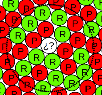
Figure 1: (Color on-line only) Crowd with relaxed (green circles) and panicking (red circles) pedestrians. The state of the pedestrian labeled with question marks depends of the amount of neighboring panicking and relaxed individuals (see Eq. 7). The circle indicate the contagious radius.

where the parameter $J$ represents an effective contagion stress (see Appendix A for details). This parameter resembles the pedestrian susceptibility to enter in panic. For simplicity we further assume that this parameter is the same for all the pedestrians.

The symbol $\langle\cdot\rangle$ represents the mean value for any short time interval (see Appendix A for details). However, for practical reasons, we will replace this mean value with the sample value $k/n$ at each time-step.

II.3 The stress decay model

The pedestrian “stress decay” corresponds to the individual’s natural relaxation process in the absence of stimuli (i.e. emotions), until he (she) settles to relaxed. This behavior is mathematically expressed through the relaxation term in Eq. (6). Thus, in the absence of stimuli (that is, vanishing values of $\mathcal{P}$), it follows from Eq. (5) and Eq. (6) that

$$v_{d}(t)=v_{d}^{\mathrm{min}}+(v_{d}^{\mathrm{max}}-v_{d}^{\mathrm{min}})\,M(0)\,e^{-t/\tau_{M}}$$ (8)

for any fixed value $M(0)$ at $t=0$, and a vanishing value of $M(t)$ long time after ($t\gg\tau_{M}$). The characteristic time $\tau$ is different from $\tau_{M}$. Ref. Ta et al. (2017) suggests that $\tau_{M}\simeq 50\,$ seconds.

The characteristic time $\tau_{M}$ may be different from the suggested value according to specific environmental factors. Eq. (8) proposes the way to handle an estimation of $\tau$ whenever the composure desired velocity $v_{d}(t_{c})$ is known ($t_{c}$ being the time required to arrive to composure). Assuming $M(0)=1$, it is straight forward that

$$\tau_{M}^{-1}=\displaystyle\frac{1}{t_{c}}\,\ln\bigg{(}\displaystyle\frac{v_{d}^{\mathrm{max}}-v_{d}^{\mathrm{min}}}{v_{d}(t_{c})-v_{d}^{\mathrm{min}}}\bigg{)}$$ (9)

II.4 Topological characterization

One of the most useful image processing technique is the computation of the Minkowski functionals. This general method, based on the concept of integral geometry, uses topological and geometrical descriptors to characterize the topology of two and three dimensional patterns.

We used this method to analyze data (images) obtained from the video of the Charlottesville incident. So, we focused the attention on the 2-D case. Three image functionals can actually be defined in 2-D: area, perimeter and the Euler characteristic. The three can give a complete description of 2-D topological patterns appearing in (pixelized) black and white images.

To characterize a pattern on a black and white image, each black (or white) pixel is decomposed into 4 edges, 4 vertices and the interior of the pixel or square. Taking into account the total number of squares ($n_{s}$), edges ($n_{e}$) and vertices ($n_{v}$), the area ($A$), perimeter ($U$) and Euler characteristic ($\chi$) are defined as

$$A=n_{s},~{}~{}U=-4n_{s}+2n_{e},~{}~{}\chi=n_{s}-n_{e}+n_{v}$$ (10)

The area is simply the total number of (black or white) pixels. The second and third Minkowski functionals describe the boundary length and the connectivity or topology of the pattern, respectively. The latter corresponds to the number of surfaces of connected black (white) pixels minus the number of completely enclosed surfaces of white (black) pixels (see Ref. Michielsen and Raedt (2001)).

III Experimental data

In this section we introduce two incidents, as examples of real life panic propagation. The first one occurred in Turin (Italy) while the other one took place in Charlottesville (USA) in 2017. We further present relevant data extracted from the corresponding videos available in the web (see on-line complementary material).

III.1 Turin (Italy)

On June 3rd 2017, many Juventus fans were watching the Champions League final between Juventus and Real Madrid on huge screens at Piazza San Carlo. During the second half of the match, a stampede occurred when one (or more) individuals shouted that there was a bomb. More than 1000 individuals were injured during the stampede, although it was a false alarm. Fig. 2 captures two moments of the panic spreading (see caption for details). The arrow in Fig. 2b points to the individual that caused the panic spreading. He will be called the fake bomber throughout this investigation.

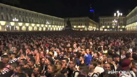
(a) Pedestrians watching the screen.

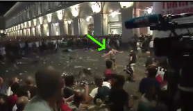
(b) Pedestrians in panic.

(c) Panic spreading.

Figure 2: (Color on-line only) (a) Snapshot of the crowd watching the football match. The screen is on the left (out of the scene). The pedestrians on the right are actually in fear due to the fake bomber. The (b) snapshot corresponds to the same scene as (a) but shifted to the right (actually, the camera appearing in this image is the one that captured the (a) image). The fake bomber appears in the scene and is indicated with a green arrow. (c) Analysis of the panic spreading among the crowd. The blue and orange profiles represent the relaxed and anxious pedestrians, respectively, associated to the (a) image (see text for details). In fact, in the (b) image we can observe (on the right of the image) the camera that captured the (a) image. The total number of contour bodies is $N=131$.

The recordings from Piazza San Carlo show how the pedestrians escape away from the “panic source”, that is, from the fake bomber. It can be seen in Fig. 2b the opening around the panic source a few seconds after the shout. The opening exhibits a circular pattern around the fake bomber. This pattern gradually slows down as the pedestrians realize the alarm being false. Approximately 20 seconds after the shout, the pedestrians calm down to the relaxed state while the opening closes.

In order to quantify the panic contagion among the crowd, we split the video into 14 images. The frame rate was 2 frames per second. Thus, the time interval between successive images was 0.5 seconds. This time interval corresponds to the acceleration time $\tau$ in the SFM.

Fig. 2c shows the profile corresponding to the first image. Any (distinguishable) pedestrian in Fig. 2a is outlined in Fig. 2c as a body contour. The contour colors represent relaxed pedestrians (i.e. blue in the on-line version) or pedestrians in panic (i.e. orange in the on-line version). The latter correspond to the individuals that suddenly changed their motion pattern. That is, individuals that turned back to see what happened or pedestrians that were pushed towards the screen (on the left) due to the movement of his (her) neighbors.

The panic spreading shown in Fig. 2c occurs from right to left, until nearly all the contour bodies switch to the panic state (i.e. orange in the on-line version). Notice, however, that a few pedestrians may remain relaxed for a while, even though his (her) neighbors have already switched to the panic state. Or, on the contrary, pedestrians in panic may be completely surrounded by relaxed pedestrians, as appearing on the left of Fig. 2c. Both instances are in agreement with the hypothesis that pedestrians may switch to a panic state according to an contagion efficiency $\mathcal{P}$. See Appendix A for details on the $\mathcal{P}$ computation within the contagion radius.

The inspection of successive images provides information on the new anxious or panicking pedestrians and the state of their current neighbors. Appendix B summarizes this information, while detailed values for the contagion efficiency $\mathcal{P}$ and the contagion stress $J$ are reported in Table 1. Notice that the data sampling is strongly limited by the total number of outlined pedestrians (that is, 131 individuals). Thus, the reported values for $t>4\,$s are not really suitable as parameter estimates because of the finite size effects. In order to minimize the size effects, we focused on the early stage of the contagion were the contagion stress $J$ seems to be (almost) stationary (see Fig. 14).

The (mean) contagion stress for the Turin incident was found to be $J=0.1\pm 0.055$ (within the standard deviation). This value appears to be surprisingly low according to explored values in the literature (see Ref. Nicolas et al. (2016)). However, we shall see in Section V that this stress is enough to reproduce real life incidents.

III.2 Charlottesville, Virginia (USA)

One person was killed and 19 injured when a car ran over into a crowd of pedestrians during an antifascist protest (Charlottesville, August 12th, 2017). The incident took place at the crossing of Fourth St. and Water St. Fig. 3a shows a snapshot of the incident (the video is provided in the supplementary material).

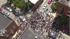
(a) Original frame.

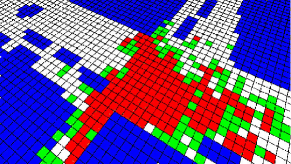
(b) Pixelated image.

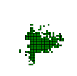
(c) Perspective correction.

Figure 3: (a) Image of the incident in Charlottesville. This image corresponds to the first frame of the video. (b) Pixelated image of the original frame. In the image we identify in blue color the obstacles, like cars and buildings. Green and red cells are occupy by one and more than one pedestrians, respectively. The street was colored in white. The line spacing was 12 pixels. The cell size was, approximately, $1.5\,\mathrm{m}\times 1.5\,\mathrm{m}$. (c) Perspective correction of the pixelated image. In green color we represents the position of the occupied cells by pedestrians. The white spaces represents the obstacles (buildings and cars) and the street.

In the video, we can see that the whole crowd gets into panic. But, we can identify two groups of pedestrians, according to the amount of information they have about the incident. The individuals near the car (say, less than 5 m) actually witnessed when the driver ran over into the crowd. However, far away pedestrians become aware that something happened among the crowd due to the fear emotions of his (her) neighbors. But, they cannot determine the nature of the incident because the car is out of their sight. Thus, the pedestrians nearer to the car have more information than the far away individuals.

The video also shows that the pedestrians close to the car stop running as soon as the car stops. On the contrary, far away individuals continue escaping after this occurs due to their lack of information.

Using the program ImageJ Rasband, W.S., ImageJ, U. S. National Institutes of Health, Bethesda, Maryland, USA, https://imagej.nih.gov/ij/, 1997-2016 , we were able to follow the trajectories of various pedestrians. As shown in Fig. 4, most of the trajectories are approximately radial to the car. Notice, however, that three individuals ran toward the car to help the other injured pedestrians.

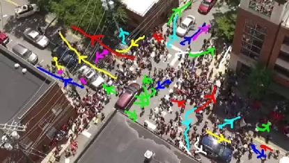
Figure 4: (Color on-line only) Trajectories for some pedestrians in panic from the Charlottesville video. The pedestrians’ positions were recorded on consecutive images, and then joined by means of the software ImageJ. The arrows represent the movement direction.

In order to obtain more experimental data, we split the video into 19 frames. The frame rate was two frames per second. We further overlapped a square grid on each frame, but taking into account the two-point perspective of each image. Each cell was colored with different colors depending if it was occupied by pedestrians, obstacles, etc (see caption in Fig. 3b for details). Finally, we performed a back-correction of the perspective for a better inspection of the grid. The result is shown in Fig. 3c.

The complete analysis of the geometrical and topological patterns appearing on the grid can be found in Section V.

IV Numerical simulations

IV.1 The simulation conditions

The Turin scenario

We mimicked the Turin incident (see Section III) by first placing 925 pedestrians inside a 21 m $\times$ 21 m square region. The pedestrians were placed in a regular square arrangement, meaning that the occupancy density was approximately 2 people/m². After their desire force was set (see below), the crowd was allowed to move freely until the pedestrian’s velocity vanished. This balance situation can be seen in Fig. 5a and corresponds to the initial configuration for the panic spreading simulation.

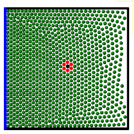
(a) Turin initial state.

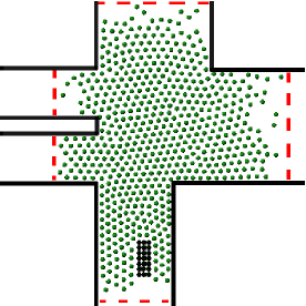
(b) Charlottesville initial state.

Figure 5: Snapshots of the initial configuration for the (a) Turin (Italy) and (b) Charlottesville (Virginia, USA) simulations. The relaxed pedestrians are represented in green circles on both images. (a) The fake bomber is represented in black, while his first neighbors are represented in red (see text for details). The blue line on the left represents the wide screen. (b) The car is represented by 21 black circles and moves from bottom to top. The solid (black) lines represent the walls and other obstacles (i.e. parked cars on the middle left of the image (see Fig. 3)). The width of the street at the bottom of the image is 8 m and at the top reaches 15 m (see red dashed lines). The street width on the left is divided into two paths of 5 m each, while the street width on the right is 13 m (see red dashed lines). Initially, the pedestrians were placed at random positions inside the region bounded by the red dashed lines.

The blue line on the left of Fig. 5a represents the wide screen mentioned in Section III.1. We assumed that the pedestrians are attracted to the screen in order to have a better view of the football match. Thus, a (small) desire force pointing towards the screen was included at the beginning of the simulation. This force equaled $m\,v_{d}/\tau$ for the standing still individuals ($v(0)=0$), according to Eq. (2). We further assumed that the pedestrians were in a relaxed state at the beginning of the simulation, and therefore, we set $v_{d}=0.5\,$m/s Parisi and Dorso (2005). This value accomplished a local density that did not exceed the maximum expected for outdoor events, say, 3-4 people/m².

The pedestrian in black in the middle of the crowd in Fig. 5a represents the fake bomber appearing in the video. He is responsible for triggering the panic contagion at the beginning of the simulations. For simplicity, we assumed that he remained still during the panic spreading process.

The pedestrians in red in Fig. 5a are responsible for shouting the alert, as they are very close to the fake bomber (less than $1\,$m). They were initially set to the panic state in the simulation (see Section IV.2 for details).

Recall that the event takes place outdoor. Piazza San Carlo, however, is surrounded by walls (as can be seen in Fig. 2a). We considered along the simulations that the crowd always remained inside the piazza and no other pedestrian were allowed to get inside during the process.

The Charlottesville scenario

The initial conditions for simulating the incident at Charlottesville are somewhat different from those detailed in Section IV.1. The pedestrians are now placed at random positions within certain limits around the street crossing (see Fig. 5b). But, in order to counterbalance the social repulsion between pedestrians, a (small) inbound desire force was set. That is, the pedestrian’s desire force pointed to the center of the crossing.

The total number of pedestrians appearing in Fig. 5b is 600. This number was computed taking into account the total number of occupied cells and the amount of pedestrians per cell of the first frame of the video (see caption of Fig. 3b for details). Due to the low image quality of Fig. 3a, we were not able to distinguish if more than two pedestrians per cell. Thus, we simply assumed that each red cell was occupied by only two pedestrians.

After setting the pedestrian’s desire force to $v_{d}=0.5\,$m/s, we allowed them to move freely towards the center of the street crossing. This instance continued until a similar profile to the one in Fig. 3a was attained.

Then, we assumed, according to the video, that the pedestrians tried to stay at a fix position. Thus, we set the desired velocity to zero and allowed the system to reach the balance state before initiating the simulation. Notice that this condition differed slightly from the Turin condition, where the desired velocity was set to $0.5\,$m/s.

The “source of panic” for the Charlottesville’s incident corresponds to the offending driver moving along the vertical direction in Fig. 5b. We modeled the offending driver as a packed group of 21 spheres, (roughly) emulating the contour of a car (see Fig. 5b). The mean mass of the packed group was set to 2000 kg. The car moved from bottom to top at 3 m/s until it reached the center of the street intersection. When this occurred, it stopped and remained fix until the end of the simulation.

As in the Turin situation, we assumed that those pedestrians very close to the car (that is, less than 1 m) entered into panic immediately, and thus, they were initially set to the panic state. When the car stopped, the “source of panic” was switched off.

The streets are considered as open boundary conditions. This means that the pedestrians are able to rush away from the crossing as far as they could.

IV.2 The simulation process

The videos that capture the panic spreading over the crowd let us classify the pedestrians into those moving relaxed or those moving anxiously. These are qualitative categories that can be easily recognized through the pedestrian’s behavioral patterns. An accurate value for the inner stress $M$ seems not to be possible from the videos. Thus, we assume that the pedestrians may be in one of two possible states: relaxed or in panic. The former means that his (her) desired velocity does not exceed a fix threshold $v_{d}^{\mathrm{lim}}$, or $M_{\mathrm{lim}}$, according to Eq. (5). The latter means that the individual surpassed this threshold.

We already mentioned in Section IV.1 that the desired velocity $v_{d}=0.5\,$m/s is in correspondence with either accepted literature values for relaxed individuals and the expected local density for approximately 900 individuals. Hence, we set $v_{d}^{\mathrm{lim}}=0.5\,$m/s as a reasonable limit for the pedestrian to be considered relaxed. This limit is supposed to be valid for either the Turin and the Charlottesville incident, since the total number of pedestrians involved in each event and the expected maximum local density are similar in both cases.

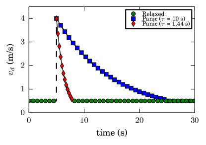
Figure 6: Time evolution of the desired velocity $v_{d}$ for a single individual. The green color corresponds to the relaxed state, while the red color corresponds to the panic state. At $t=5\,$s the $v_{d}$ switches from $0.5\,$m/s to $4\,$m/s due to panic contagion. No further stimulus is received after the contagion. The desired velocity decays exponentially from $t>5\,$s resembling the stress decay. The red diamond and blue square symbols represents two exponential characteristic times: $\tau$ = 1.44 s and $\tau$ = 10 s, respectively. At $t\simeq 10\,$s and $t\simeq 25\,$s (depending the value of $\tau$) the desired velocity attains $v_{d}^{\mathrm{lim}}=0.5\,$m/s and the individual returns to the relaxed state.

For simplicity, $v_{d}^{\mathrm{min}}$ and $v_{d}^{\mathrm{max}}$ (Eq. (5)) were set to zero and $4\,$m/s, respectively, in all the simulations. The maximum velocity $v_{d}^{\mathrm{max}}=4\,$m/s corresponds to reasonable anxiety situations appearing in the literature Helbing and Molnár (1995); Frank and Dorso (2011, 2015); Sticco et al. (2017).

Fig. 6 illustrates the time evolution for the desired velocity $v_{d}(t)$ of an individual who switches from the relaxed state to the panic state (see caption for details). Notice that the increase in the inner stress is implemented as an (almost) instantaneous change in his (her) desired velocity due to panic contagion. This corresponds to the contagion process. Once in panic, however, the stress decay phenomenon applies, regardless of any other neighbor expressing fear. The stress decay stops when the individual settles to the relaxed state, that is, when the $v_{d}$ returns back to $0.5\,$m/s. When this occurs, the pedestrian moves randomly at this desired velocity until the end of the simulation.

In order to determine the experimental value of the characteristic time $\tau$, we measured the time required by an anxious pedestrian to recovers his (her) relaxed state ($t_{c}$). According the analysis of the videos, in the Turin’s case anxious pedestrians returns to a relaxed state after 20 seconds.

But, in the Charlottesville case, near pedestrians (less than 5 m) from the car relaxed after 3 seconds. However, far away pedestrians arrive to the relaxed state after 20 seconds. Recall from Section III.2, that near individuals to the car has more information about the incident nature than far away ones. Thus, when the car stops, near individuals recovers his relaxed state unlike the far away pedestrians that continues in panic.

We computed the experimental value of the characteristic time $\tau$ for each scenario using Eq. (9) with $v_{d}^{\mathrm{min}}$ = 0 m/s, $v_{d}^{\mathrm{max}}$ = 4 m/s and $v_{d}(t_{c})$ = 0.5 m/s. In the Turin’s case, $\tau$ equals, approximately, to 10 seconds, while in the Charlottesville’s case the characteristic time equals to 1.44 seconds and 10 seconds for near and far away pedestrians, respectively.

Notice that an anxious pedestrian has more or less “influence” over his neighbors according his (her) information level about the incident. That is, for example an individual near to the car can spread his (her) fear emotion over a relaxed pedestrian during, only, 3 seconds. In other words, during the time that were in panic ($t_{c}$).

The panic contagion process

The panic contagion process was implemented as follows. First, we associated an effective contagion stress $\mathcal{P}^{(i)}$ to each relaxed individual, according to Eq. (7). That is, we computed the fraction of neighbors in the panic state $k$ to the total number of neighbors $n$ within a fix contagion radius of $2\,$m (from the center of mass of the corresponding relaxed pedestrian $i$). Second, we randomly switched the relaxed pedestrians to the panic state, according to the associated effective contagion stress $\mathcal{P}^{(i)}$. The $\mathcal{P}^{(i)}$ values were updated at each time step (say, $0.05\,$s).

Notice that this contagion process may be envisaged as a Susceptible-Infected-Susceptible (SIS) process. The Susceptible-to-Infected transit corresponds to the (immediate) increase of $v_{d}$ from $0.5\,$m/s to $4\,$m/s (with effective contagion stress $\mathcal{P}^{(i)}$). The Infected-to-Susceptible transit corresponds to the stress decay from $4\,$m/s back to $0.5\,$m/s.

We want to remark the fact that the emotions received by an individual in the panic state were neglected, and thus, did not affect the stress decay process. This should be considered a first order approach to the panic contagion process.

Simulation software

The simulations were implemented on the Lammps molecular dynamics simulator Plimpton (1995). Lammps was set to run on multiple processors. The chosen time integration scheme was the velocity Verlet algorithm with a time step of $10^{-4}\,$s. Any other parameter was the same as in previous works (see Refs. Frank and Dorso (2015, 2011)).

We implemented special modules in C++ for upgrading the Lammps capabilities to attain the “social force model” simulations. We simulated between 60 and 90 processes for each situation (see figures caption for details). Also, the processes lasted between 10 s and 20 s according each analysis. Data was recorded at time intervals of 0.05 s. The recorded magnitudes were the pedestrian’s positions and their emotional state (relaxed or anxious) for each evacuation process.

V Results

This section exhibits the results obtained from either real life situations and computer simulations. Two sections enclose these results in order to discuss them in the right context. We first analyze the Turin case (Section V.1), while the more complex one (Charlottesville, Virginia) is left to Section V.2.

V.1 Turin

V.1.1 The contagion stress parameter

As a first step, we measured the mean number of anxious pedestrians during the first $20\,$s of the escaping process for a wide range of contagion stresses ($J$). This is shown in Fig. 7. As can be seen, the number of anxious pedestrians increases for increasing contagion stresses. That is, as pedestrians become more susceptible to the fear emotions from his (her) neighbors, panic is allowed to spreads easily among the crowd.

The fraction of pedestrians that switch to the anxious state exhibits three qualitative categories as shown in Fig. 7. For $J$ ranging between 0 to 0.01, no significant spreading appears. But this scenario changes rapidly for the $J$ (intermediate) range between 0.01 and 0.03. The slope in Fig. 7 experiences a maximum throughout this interval. However, if the stress becomes stronger (say, above 0.03), the majority enters into panic regardless of the precise value of $J$. A seemingly threshold for this is around $J=0.04$.

Notice that Fig. 7 is in agreement with the experimental Turin value for the mean contagion stress ($J=0.100\pm 0.055$, see Section III). The panic situation at Piazza San Carlo, as observed from the videos, shows that all the pedestrians moved to the panic state. The snapshot in Fig. 2b illustrates the situation a while after the (fake) bomber called for attention.

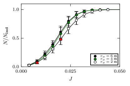
Figure 7: Normalized number of anxious pedestrians during the first 20 s of the escaping process as a function of the contagion stress $J$ for $r_{o}$ = 2 m, 4 m and 6 m. $N$ is the number of anxious pedestrians. The plot is normalized with respect to the total number of individuals ($N_{ind}$ = 925). $J$-values of 0.01 and 0.02 are indicated in red color (and squared symbols). Mean values were computed from 60 realizations. The error bars corresponds to $\pm\sigma$ (one standard deviation).

The panic contagion shown in Fig. 7 does not appear to change significantly for increasing contagion radii. We explored situations enclosing only first neighbors ($2\,$m) to situations enclosing as far as $6\,$m. The number of pedestrians in panic always attained a maximum slope at almost the same $J$ value for all the investigated situations. This value (close to 0.025) seems to be an upper limit for any weak panic spreading situation, or the lower limit for any widely spreading situation. We may hypothesize that two qualitative regimes may occur for the panic propagation in the crowd.

Following the above working hypothesis, we turned to study any morphological evidence for both regimes in Section V.1.2 .

V.1.2 The escaping morphology

Our next step was to examine the anxious pedestrian’s spatial distribution for the Piazza San Carlo scenario. The corresponding videos show that the individuals tried to escape radially from the (fake) bomber (see Fig. 2b). Thus, the polar space binning (i.e. cake slices) centered at the (fake) bomber seemed the most suitable framework for inspecting the crowd morphology piece-by-piece. We binned the piazza into $N_{\mathrm{bins}}=30$ equally spaced pieces as shown in Fig. 5a. The angle between consecutive bins was $\varphi=360^{\circ}$/$N_{\mathrm{bins}}=12^{\circ}$.

Fig. 8 exhibits the number of occupied bins or slices (normalized by the total number of bins) occupied at least by one anxious pedestrian. Three different contagion situations are represented there. These situations attain the qualitative categories mentioned in Section V.1.1. That is, $J=0.01$ for low panic spreading, $J=0.02$ for an intermediate spreading and $J=0.09$ for wide panic spreading (see caption of Fig. 8 for details).

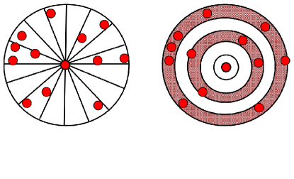
(a)

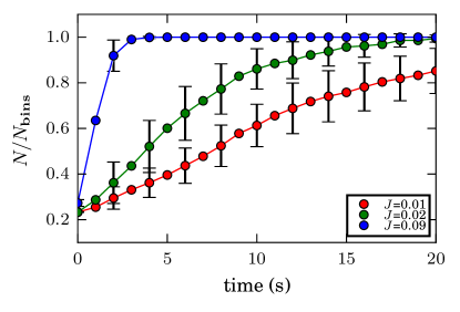
(b)

Figure 8: (a) Schematic representation of the radial (left) and circular (right) bins (see text for more details). The red circles represent the position of many anxious pedestrians. The fake bomber is place at the center of the region. (b) Fraction of occupied radial bins by anxious pedestrians vs. time (in seconds) for $J=0.01$, 0.02 and 0.09. $N$ is the number of occupied radial bins (see text for more details). The plot is normalized with respect to the total number of radial bins ($N_{\mathrm{bins}}=30$). Mean values were computed from 60 realizations. The error bars corresponds to $\pm\sigma$ (one standard deviation).

According to Fig. 8, the number of occupied bins (slices) increases monotonically during the escaping process. This means that panic propagates in all directions (from the bomber) until nearly all the slices become occupied. However, the slopes for each situation are quite different. As the contagion stress $J$ increases, the bins become occupied earlier in time (higher slopes). For the most widely spread situation ($J=0.09$) all the slices become occupied before the first 5 seconds, meaning that we may expect escaping pedestrians in any direction during most of the contagion process.

Fig. 9 represents the aforementioned three situations after $15\,$s since the (fake) bomber shout (see caption for details). These snapshots may be easily compared with the corresponding slice occupancy plot exhibited in Fig. 8.

Fig. 9a corresponds to the lowest contagion stress ($J=0.01$). We can see a somewhat “branching” pattern for those pedestrians in panic (red circles). That is, a branch-like configuration is present around the (fake) bomber. From the inspection of the whole process through an animation, we further noticed that these branches could be classified into two types (see below). The “branching” profile is also present in Fig. 9b for $J=0.02$, although this category exhibits an extended number of pedestrians in panic. The highest contagion stress category ($J=0.09$), instead, adopts a circular profile (see Fig. 9c).

The “branching” profile observed for $J=0.01$ and $J=0.02$ may be associated to the positive slopes in Fig. 8. Likewise, the circular profile for $J=0.09$ can be associated to the flat (blue) pattern therein. This suggests, once more, that two qualitative regimes may occur for the panic propagation in the crowd, as hypothesized in Section V.1.1. Low contagion stresses correspond to the (qualitative) branch-like regime, while high contagion stress correspond to the (qualitative) circular-like regime. The snapshot in Fig. 2b clearly shows a circular-like regime, as expected for the obtained experimental value of $J$.

The branching-like profile in Piazza San Carlo is not completely symmetric since the pedestrian’s density is higher near the screen area (on the left of Fig. 1 and Fig. 9) than in the opposite area. The pedestrians near the screen can not move away as easily as those in the opposite direction. Thus, the panic contagion near the screen occurs among almost static pedestrians, while the contagion on the opposite area occurs among moving pedestrians. Both situations, although similar in nature, produce an asymmetric branching. We labeled as passive branching the one near the screen, and active branching the one in the opposite direction.

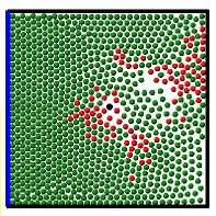
(a) $J=0.01$

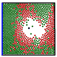
(b) $J=0.02$

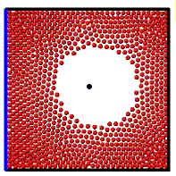
(c) $J=0.09$

Figure 9: Snapshots of different escaping processes for three values of contagion stress in the first 15 seconds. The different colors of the circles represents the anxiety state of each pedestrian. Relaxed and panic pedestrians are represents in green and red circles, respectively. The fake bomber is place at the center of the region and is represented in black circle. Relaxed pedestrians desire to reach the screen located on the left (blue line).

It may be argued that since the $J=0.09$ pattern in Fig. 8 exhibits a positive slope at the very beginning of the contagion process and a vanishing slope a few seconds after (say, $5\,$s), the association of branch-like to low $J$, and circular-like to high $J$, is somehow artificial. This is not true, as explained below.

We further binned the piazza into circular sectors around the (fake) bomber as shown in Fig. 8 (see caption for details). We carried out a similar analysis as in Fig. 8, but for the sectors. Say, we computed the number of occupied sectors at each time-step. The results were similar as for the slices (not shown). This means that both (slices and sectors) behavioral patterns are strongly correlated (for any fixed $J$).

The number of occupied sectors, somehow, indicates the speed of the radial propagation. Thus, the circular-like profiles correspond to higher speeds than the branch-like profiles, and consequently, it is not possible to associate low stress to circular profiles (or high stress to branch profiles). The propagation velocity will simply not match. Indeed, the circular profile appears only at high contagion stresses (for this piazza geometry).

We may summarize the investigation so far as follows. The panic spreading dynamic may experience important (qualitative) changes according to the “efficiency” of the alerting process between neighboring pedestrians. This is expressed by the contagion stress parameter $J$. The Piazza San Carlo video, and our simulations, show that panic propagates weakly for low values of $J$. This produces a branch-like, slow panic spreading around the source of danger (for a simple geometry). However, if $J$ exceeds (approximately) 0.025 the panic contagion spreads freely in a circular-like profile (for a simple geometry). The propagation also becomes faster.

It should be emphasized that $J\sim 0.025$ is an approximate threshold, but well formed circular-like profiles appear, in our simulations, for stresses above 0.03. Stresses beyond 0.04 exhibit similar profiles as those for $J\sim 0.04$. These results are valid for contagion radii between $2\,$m and $6\,$m.

Recall that the increase in the “inner stress” is the underneath mechanism allowing the panic to spread among the crowd. The “emotional decay”, however, seems not to play a relevant role in Piazza San Carlo (and in our simulations). This is because the experimental characteristic time for the “emotional decay” is $\tau=10\,$s, allowing anxious pedestrians to settle back to the relaxed state after $20\,$s (see Fig. 6).

We will discuss in Section V.2 a geometrically complex situation where either the “inner stress” and the “emotional decay” plays a relevant role.

V.2 Charlottesville, Virginia

V.2.1 Density contour

We first computed the discretized density pattern at the beginning of the simulation process in order to compare it with the video pattern shown in Fig. 3b. We used the same cell size as in Fig. 3b ($1.5\,\mathrm{m}\times 1.5\,\mathrm{m}$). The corresponding contour density map can be seen in Fig. 10.

Fig. 10 and Fig. 3b exhibit the same qualitative profiles. Also, the pedestrian occupancy per cell is similar on both figures. Notice that the middle of the region is occupied by two or more pedestrians per cell. The boundary cells, though, are occupied by a single pedestrian per cell in both figures. So, we may conclude that our initial configuration is qualitative and quantitative similar to the one in the video.

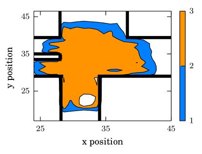
Figure 10: Mean density contour lines computed from 90 processes. This density map corresponds to the initial state of the Charlottesville simulation. The scale bar on the right is expressed in people/m². The black lines represent the walls. The white circular shaped pattern at the bottom of the image corresponds to the car location. The contour lines were computed on a squared grid of $1.5\,\mathrm{m}\times 1.5\,\mathrm{m}$ and then splined to get smooth curves. Level colors can be seen in the on-line version only.

V.2.2 The contagion stress parameter $J$

Our next step was, as in the Turin case, to compute the mean number of anxious pedestrians during the first 15 seconds of the escaping processes as a function of the contagion stress ($J$). The results can be seen in Fig. 11.

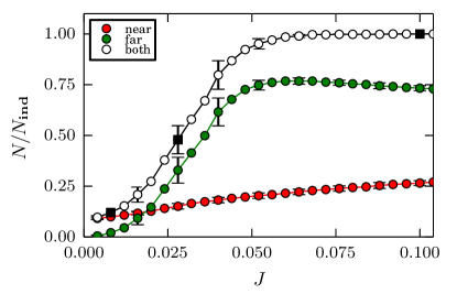
(a)

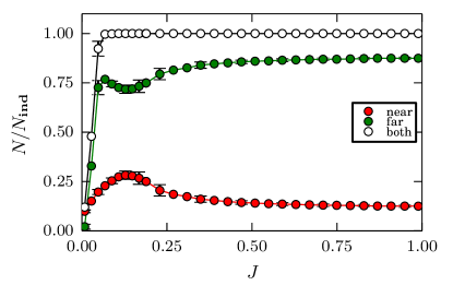
(b)

Figure 11: Normalized number of anxious pedestrians during the first 15 s of the escaping process, as a function of the contagion stress $J$. $N$ is the number of anxious pedestrians. The plot is normalized with respect to the total number of individuals ($N_{ind}$ = 600). The red color corresponds to panicking pedestrians close to the car (less than 5 m), while the green color corresponds to those far away from the car (more than 5 m). The white symbols correspond to the (normalized) set of all individuals in panic. Results for $J$ = 0.010, 0.028, and 0.1 are indicated in black color (and squared symbols). Mean values were computed from 60 realizations. The error bars corresponds to $\pm\sigma$ (one standard deviation).

We observe that, likewise the Turin case, that the total number of anxious pedestrians (hollow symbols and black line) increases for increasing contagion stresses. From the comparison between Fig. 7 and Fig. 11a we may realize that both situations exhibit the same qualitative patterns for the total number of anxious pedestrians. However, the slope for the Charlottesville situation is somewhat lower with respect to the Turin situation (see Fig. 7).

In order to explain this slope discrepancy we computed, separately, the (mean) number of anxious pedestrians close to the car (i.e. source of panic) and those far away from the car. Recall from Section IV that the former correspond to better informed pedestrians than the latter. The computation of the number of “near” anxious pedestrians actually include those pedestrians that get into panic very close to the car (less than 1 m).

We may recognize from Figs. 11a and 11b the same three qualitative categories mentioned in Section V.1.1, according to the contagion stress value. Notice, however, that the anxious pedestrians now settle to the relaxed state after 3 seconds (if near the car) or 20 seconds (if far away from the car). We will examine these regimes in the following sections.

The low contagion stress regime

For $J$ ranging between 0 to 0.02, most of the pedestrians that get anxious are close to the car, while the far away pedestrians remain in a relaxed state. This means that panic does not spread homogeneously over all the crowd.

Recall from Section IV.1 that individuals located very close to the car (less than 1 m) get into panic immediately. So, as the car moves across the crowd, the panic propagates first over these nearby individuals. This explains why, in Fig. 11a, there is a small number of anxious pedestrians for extremely low contagion stresses ($J$ $\sim$ 0).

Notice that this small group of anxious pedestrians represent the first source of panic inside the crowd (regardless of the car). As the susceptibility to fear emotions increase, their neighbors get into panic. But, due to their rapid fear decay (3 seconds), their influence on the surrounding neighbors is low. This is the reason for the smooth increment of the near anxious pedestrians.

Besides, we can observe from Fig. 11a that the number of far away pedestrians getting into panic is not significant. Any pedestrian located far away from the car may only get anxious if panic surpasses his (her) contagion radius. So, if the number of “near” anxious pedestrians is low while also relaxing quickly (i.e. 3 seconds), then the “probability” that panic reaches far away pedestrians from the car is indeed very low. This explains the low number of far away pedestrians that get anxious during this interval (less than 0.02).

The intermediate contagion stress regime

The panic spreading scenario changes if $J$ ranges between 0.02 and 0.05. Along this interval, the total number of anxious pedestrians (white circles) increases abruptly. We can observe that this corresponds essentially to the increase in the amount of far away anxious pedestrians. Indeed, the number of near anxious pedestrians shown in Fig. 11a exhibits a smooth increment that cannot explain the abrupt increase of the total number of anxious individuals.

Notice that an increment in the number of anxious “far away” pedestrians becomes possible (at high contagion stresses) due to the significant time window that they spend surrounded by other “far away” anxious pedestrians (say, 20 seconds). Thus, the compound effect of high susceptibility to fear emotions and the long lasting time decays ($t_{c}$) explains the sharp increase in the number of anxious pedestrians.

The high contagion stress regime

Finally, if the contagion stress becomes intense (say, above 0.05), most of the individuals get into panic regardless of the precise value of $J$. Thus, as in the Turin situation, we may consider a seemingly threshold for this regime around $J$ = 0.07. Fig. 11b shows, however, that two noticeable behaviors appear whether the contagion stress is (roughly) below $J$ = 0.2 or not (despite the fact that the majority enters into panic).

Below $J$ = 0.2, the number of pedestrians that get into panic near the car increases for increasing contagion stresses, while above this threshold the corresponding slope in Fig. 11b changes sign. The number of far away anxious pedestrians exhibit, though, a small “U” shape and a positive slope for $J\gg 0.2$ (see Fig. 11b).

The increase in the number of individuals that get into panic near the car just below the threshold $J$ = 0.2 attains for the increase in the susceptibility to fear emotions. But, above $J$ = 0.2, the situation is somewhat different. The contagion stress is so intense that panic propagates rapidly into de crowd. People standing as far as 5 m from the car may switch to an anxious state, and thus, they get into panic before the car (i.e. the source of panic) approaches them. Our simulation movies (not shown) confirm this phenomenon. We further realized that many of the anxious individuals located near the car and computed into the red curve in Fig. 11b at $J\leq 0.2$ may actually move to the green curve at extremely intense stresses $J\gg 0.2$.

The above research may be summarize as follows. We identified three scenarios according to the contagion stress. If the susceptibility to fear emotions is low (below 0.02), the panic spreads over a small group of pedestrians located very close to the car. In the case of an intermediate contagion stress ($J$ between 0.02 and 0.05), the number of pedestrians that get into panic far away from the car increases abruptly. Above $J$ = 0.05, the panic spreads over all the crowd.

The propagation velocity of the fear among the crowd is related to the contagion stress ($J$). As the susceptibility to fear emotions increases, the panic spreading velocity also increases. So, if pedestrians are very susceptible to fear emotions, just a small number of individuals is capable of spreading panic over the whole crowd.

V.2.3 The escaping morphology

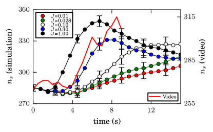
(a) Area.

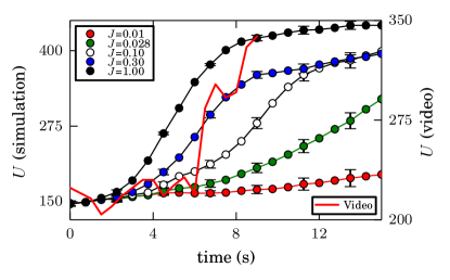
(b) Perimeter.

Figure 12: Minkowski functionals corresponding to the (a) area ($n_{s}$) and (b) perimeter ($U$) (see Section II.4 for more details). The red, green, white blue and black circles corresponds to the Charlottesville simulation. The red line corresponds to the experimental data extracted from the video incident. In both cases, the cell area was 1.5 m². The duration of the Charlottesville video was 10 seconds. Mean values were computed from 90 realizations. The error bars corresponds to $\pm\sigma$ (one standard deviation).

In Section V.2.2 we computed the total number of anxious pedestrians as a function of the contagion stress $J$. Now, we examine the pedestrian’s spatial distribution. We computed the Minkowski functionals (area and perimeter) for different contagion stresses. The results are shown in Fig. 12.

The examined situations attain the same qualitative categories mentioned in Section V.2.2. That is, $J$ = 0.01 for low panic spreading and $J$ = 0.028 for an intermediate spreading, and the two cases ($J$ = 0.1 and $J$ = 0.3) for the highly intense situation. We also analyzed the limiting case ($J$ = 1). No distinction was made at this point between relaxed or anxious pedestrians.

Recall from Section II.4, that the area is the number of occupied cells by, at least, one pedestrian. Fig. 12a shows two qualitatively different patterns, one before the first 4 seconds and the other one after this time period. The former exhibits a slightly negative slope, while a positive slope can be seen in the latter (at least for a short time period).

The first 4 seconds in the contagion process correspond to the time period since the car strikes against the crowd until it stops. So, we may associate the decrease in the area with the movement of the pedestrians next to the car. The process animations actually show that these individuals group themselves as the car moves towards the crowd.

The slope changes sign after the first 4 seconds, meaning an increase of the occupied area (see Fig. 12a). This corresponds, according to our animations (not shown), to pedestrians running away from each other. The greater the contagion stress, the sharper the slope. Since these slopes represent somehow the escaping velocity, Fig. 12a expresses the fact that people try to escape faster as they become more susceptible to fear emotions (at least during this short time period).

Fig. 12b exhibits the results for the computed perimeter. This functional informs us on the length of the (supposed) boundary enclosing the crowd. Unlike the area, the perimeter appears as an increasing function of time (for the inspected values of $J$). Furthermore, as the susceptibility to fear emotions increases, the faster the perimeter widens.

The real life data included in Fig. 12 matches (qualitatively) the simulated patterns. Indeed, simulations corresponding to high contagion stresses appear to match better. Specifically, the Minkowski functionals computed for $J$ = 0.30 exhibit the best matching patterns. Notice, however, that the scales of the experimental data and our simulations are different (see Fig. 12). This scale discrepancy is entirely due to the differences in the size of the occupancy cells corresponding to experimental data and to our simulations.

We finally examined the process animations for low ($J$ = 0.01), intermediate ($J$ = 0.028) and high ($J$ = 0.3) contagion stresses separately. These values correspond to the symbols in black color in Fig. 11. The complementary snapshots are shown in Fig. 13, captured after 10 seconds from the beginning of the process. We chose this time interval in order to differentiate the three situations more easily (see caption for details).

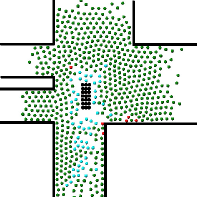
(a) $J=0.01$

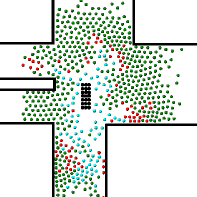
(b) $J=0.028$

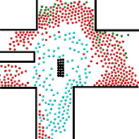
(c) $J=0.3$

Figure 13: Snapshots of different escaping processes for low ($J$ = 0.01), intermediate ($J$ = 0.028) and high ($J$ = 0.3) contagion stress in the first 10 seconds. The different colors of the circles represents the anxiety state of each pedestrian. Relaxed and panic pedestrians are represents in green and red circles, respectively. The cyan circles represents the recovered pedestrians. That is, individuals that in the past were in panic but now are relaxed due the stress decay. The offending driver is represented by black circles. The solid lines represents the walls and the row of cars located on the middle left of the image (see Fig. 3).

Fig. 13a corresponds to the lowest contagion stress ($J$ = 0.01). As already shown from Fig. 11a, only a small number of pedestrians gets into panic (due the low susceptibility to fear emotions). These pedestrians are colored in cyan in Fig. 13a (on-line version only), and correspond to people standing close to the car path. No dramatic differences appear between the profiles shown in Fig. 5b and Fig. 13a. Thus, we may expect a smooth slope for the Minkowski functionals (see Fig. 12).

Fig. 13b shows a somewhat different scenario due to $J$ = 0.028 (the intermediate contagion stress). We realize that an increasing number of pedestrians are now in panic. Many pedestrians that appeared as relaxed in Fig. 13a, have now become anxious because of the fear emotions from the individuals located near the car. However, the occupied area did not change significantly from Fig. 13a. The perimeter, instead, is expected to increase because of the voids left back by the panicking pedestrians inside the crowd (see the red circles in the on-line version of Fig. 13b).

The more stressing scenario in shown in Fig. 13c. The whole crowd gets into panic for $J=0.3$. This situation is comparable to the Turin incident (above $J$ = 0.09), despite the obvious geometrical differences. Thus, qualitatively speaking, Fig. 4 and Fig. 13c show “similar” crowd profiles.

A few conclusions can be outlined from the above analysis. As in the Turin situation, we found different scenarios according the pedestrian’s susceptibility to fear emotions. For low contagion stresses, the panic spreads over a small group of pedestrians standing close to the source of panic (the car). As the contagion stress ($J$) increases, the influence of these nearby individuals on their neighbors become more relevant. Thus, more pedestrians get into panic. If $J$ is above 0.05, the fear spreads over all the crowd.

Despite the fact that above $J$ = 0.05 all the pedestrians becomes in panic, there are two qualitatively different regimes, bounded by a threshold at (roughly) $J$ = 0.2. We found that below $J$ = 0.2, the role of the pedestrians near the source of panic (say, the better informed pedestrians) is a relevant one, since they are the mean for propagating panic deep inside de crowd. But, above $J$ = 0.2, the contagion stress is so intense that panic propagates rapidly into the crowd even though a minimum number of individuals near the car get into panic.

VI Conclusions

The contagion of panic in a crowd is usually thought to propagate like a disease among a social group. But reliable parameters for properly testing this hypothesis are not currently available. This investigation introduced two real panic-contagion events, in order to arrive to a trusty model for the panic propagation. Our work was carried out in the context of the “social force model”.

The contagion of panic offered a challenge to the emotional mechanism operating on the pedestrians. We only included the “inner stress” and “stress decay” as the main processes triggered during a panic situation. Although the simplicity of this model, we attained fairly good agreement with the real panic-contagion events.

We handled the coupling mechanism between individuals through the contagion stress parameter $J$. This parameter appears to be responsible for increasing the “inner stress” of the individuals. Our first achievement was getting a real (experimental) value for $J$. The value for the Piazza San Carlo event was $0.1\pm 0.055$.

We further noticed through computer simulations that $J$ controls the contagion dynamics. The Piazza San Carlo event illustrates the dynamic arising for high values of $J$, where everyone moves away from the source of stress. However, this might not be the case for low values of $J$. Only a small number of pedestrians will escape from danger, although many will roughly stay at their current position. The whole impression will be like random “branches” (the pedestrians in panic) moving away from the source of danger. We actually concluded that $J\sim 0.03$ is roughly the limit between both dynamics.

Our simulations attained qualitatively correct profiles for the escaping crowd either at Piazza San Carlo and the Charlottesville street crossing. But these profiles are geometry-dependent, and therefore, not a unique profile could be established for any value of $J$ at different incidents. We know (for now) that geometries similar to Piazza San Carlo may produce branch-like profiles ($J<0.03$) or circular-like profiles ($J>0.03$).

The “stress decay” depends on the nature of the source of panic (say, whether if it corresponds to a fake alert or not) and the amount of information that the pedestrians get from this source. That is, far away pedestrians from the igniting point of panic (fake bomber in the Turin situation, or the offending driver in the Charlottesville situation) may not have enough information on the nature of the incident, but nearby pedestrians may get a more precise picture of the incident. The cleared this picture becomes to them, the faster they are allowed to settle down, and thus, the shorter the characteristic decay time.

We realized, however, that a shorter characteristic time actually prevents the panic from spreading. This was not the case at the Piazza San Carlo, since the fake bomber was not (directly) at the sight of the pedestrians (who where watching the football match). The Charlottesville incident, however, exhibited two groups of individuals, according to the available information. We noticed that the group near the source of danger attained a shorter $\tau$ than the others, preventing this group from escaping.

What we learned from the street crossing incident at Charlottesville is that the resulting pedestrian’s dynamic is a consequence of the competing effects of the “inner stress” (increased by contagion stimuli) and the “stress decay”. Both are essential issues for a trusty contagion model. The parameters $J$ and $\tau$ appear as the most relevant ones within our model.

The $J$ and $\tau$ parameters may not always be available because of poor recordings or missing data. We experienced this difficulty with the video of the Charlottesville incident. But the experimental geometrical functionals, like the area or the perimeter, allowed the estimate of $J$ by comparison with respect to simulated data ($J\sim 0.3$).

We want to remark that different contagion radii (between $2\,$m and $6\,$m) did not produce significant changes on our simulations. This was unexpected, and thus, we may speculate that “spontaneous” contagion out of the usual contagion range may not produce dramatic changes, if the probability of “spontaneous” contagion is small.

Appendix A The contagion efficiency

Any individual among the crowd may increase his (her) anxiety level if his (her) neighbors are in panic. This is actually the propagation mechanism for panic: one or more pedestrians express their fear, alerting the others of imminent danger. The latter may get into panic and thus, a “probability” exists for getting into panic.

We hypothesize that the “probability to danger” (contagion efficiency) is the cumulative effect of the alerting neighbors. That is, if $k$ pedestrians among $n$ neighbors are expressing fear, then the contagion efficiency $\mathcal{P}_{n}$ of an individual is

$$\mathcal{P}_{n}=p_{n}(1)+p_{n}(2)+...+p_{n}(n)$$ (11)

where $p_{n}(k)$ represents the contagion efficiency of $k=1,2,...,n$ pedestrians (among $n$ neighbors) expressing fear. The distribution for $p_{n}(k)$ is a Binomial-like distribution if any neighbor expresses panic with fixed contagion efficiency $p$, regardless of the feelings of other neighbors. If the feelings of any neighbor (among $n$ pedestrians) is not completely independent of the other neighbors, $p_{n}(k)$ should be assessed as a Hypergepmetric-like distribution.

For the purpose of simplicity we assume that the Binomial-like distribution is a valid approximation for the $p_{n}(k)$ computation. Consequently,

$$\mathcal{P}_{n}=\displaystyle\sum_{k=1}^{n}\left(\begin{array}[]{c}n\\ k\\ \end{array}\right)p^{k}(1-p)^{n-k}=1-(1-p)^{n}$$ (12)

The mean value of neighbors expressing fear $\langle k\rangle$ is $np$. Thus,

$$\mathcal{P}_{n}=1-\bigg{(}1-\displaystyle\frac{\langle k\rangle}{n}\bigg{)}^{n}$$ (13)

It is worth noting that this expression holds for a fix value of $n$. That is, the contagion efficiency $\mathcal{P}_{n}$ is conditional to the amount of neighboring individuals $n$. The contagion efficiency for any number of neighbors $n=1,2,...,M$ is

$$\mathcal{P}=\displaystyle\sum_{n=1}^{M}\mathcal{P}_{n}\,\pi_{n}$$ (14)

where $\pi_{n}$ means the contagion efficiency that there are $n$ neighbors surrounding the anxious pedestrian. Notice that the expression (14) neither includes the term for $n=0$, nor the terms above $M$. The situation $n=0$ is not considered here since it corresponds to a “spontaneous” contagion to danger. The situation $n>M$ corresponds to far away individuals, and thus, not really capable of alerting of danger. The limiting value $M$, however, is supposed to be related to a pertaining distance and the the crowd packing density.

There is no available information on the values of $\pi_{n}$, although it may be written as the ratio $\pi_{n}=z_{n}/M$ (number of current neighbors with respect to the maximum number of neighbors).

Recalling Eq. (13), the contagion efficiency $\mathcal{P}_{n}$ may be expanded as

$$\mathcal{P}_{n}=1-(1-np+...+p^{n})=p\,f_{n}(p)$$ (15)

The function $f_{n}(p)$ stands for the summation

$$f_{n}(p)=n-\displaystyle\frac{n(n-1)}{2}\,p+...+p^{n-1}$$ (16)

Each contributing terms in $f_{n}(p)$ may be envisage as the alert to danger due to groups of individuals of increasing size (for a fix number of neighbors $n$). Notice, however, that the expression (16) holds if the feelings between neighboring pedestrians are completely independent. Otherwise, the function $f_{n}(p)$ should be considered unknown.

The overall contagion efficiency reads

$$\mathcal{P}=\displaystyle\sum_{n=1}^{M}\displaystyle\frac{z_{n}}{M}\,\displaystyle\frac{\langle k\rangle}{n}\,f_{n}(p)\simeq J\,\bigg{\langle}\displaystyle\frac{k}{n}\bigg{\rangle}$$ (17)

where $J$ represents an effective stress for the propagation, since it expresses in some way the efficiency of the alerting process. That is, no panic propagation will occur for vanishing values of $J$, while the pedestrian susceptibility to fear emotions will become more likely as $J$ increases. The stress $J$ may depend, however, on the probability $p$. Appendix B shows that this dependency is weak enough to be omitted in a first order approach.

The fraction $\langle k/n\rangle$ corresponds to the mean fraction of neighbors expressing fear with respect to the total number of neighbors. This mean fraction is computed over all the possible number of neighbors, according to Eq. (17).

Appendix B The sampling procedure for Turin

The effective stress $J$ may be evaluated from any real life situation. Details on the sampling procedure for the Turin incident at Piazza San Carlo are given in Section III.1.

As a first step, we identified those individuals that switched to the panic state along the image sequence. We also identified the surrounding pedestrians for each anxious individual, and labeled them as neighboring individuals (regardless of their current anxiety state). For simplicity, we used the same profile (shown in Fig. 2c) throughout the image sequence.

The mean fraction $\langle k/n\rangle$ was obtained straight forward from this data. Table 1 exhibits the corresponding results (see second column).

Table 1: Data provided from the Turin video (see Section III.1 for details). Samples were taken at 0.5 s time intervals. The second column shows the number of pedestrians $n_{p}$ that switched to the panic state at the corresponding time stamp. The third column exhibits the (mean) ratio between neighbors in panic with respect to the surrounding neighbors. The fourth column corresponds to the contagion efficiency $\mathcal{P}$ computed as a “no-replacement” procedure (see text). The last column corresponds to the contagion stress $J$ computed from the third and fourth columns. The total number of individuals was $N=131$.

$t$	$n_{p}$	$\langle k/n\rangle$	$n_{p}/(N-N_{p})$	$J$
0.5	1	0.17	0.0077	0.0453
1.0	1	0.20	0.0077	0.0385
1.5	5	0.43	0.0391	0.0909
2.0	5	0.42	0.0406	0.0967
2.5	2	0.13	0.0169	0.1300
3.0	4	0.55	0.0345	0.0627
3.5	6	0.36	0.0536	0.1489
4.0	13	0.64	0.1226	0.1916
4.5	11	0.68	0.1183	0.1740
5.0	10	0.52	0.1219	0.2344
5.5	22	0.63	0.3055	0.4849
6.0	29	0.90	0.5800	0.6444
6.5	15	0.88	0.7143	0.8117

Notice that the surrounding pedestrians actually correspond to the most inner ring of pedestrians enclosing the anxious individual, but not the ones within a certain radius. This radius, however, can be estimated from the (mean) packing density of the crowd.

The anxious pedestrians at the border of the examined area of Piazza San Carlo (see ) are not included in Table 1 since it was not possible to identify all of their surrounding pedestrians.

The fraction of the anxious pedestrians $n_{p}$ to the total number of individuals $N$ is a suitable estimate for the overall contagion efficiency $\mathcal{P}$. However, as panic propagates, the acknowledged anxious pedestrians $n_{p}$ diminish because the number of previously relaxed individuals reduces inside the analyzed area. Thus, the estimate of $\mathcal{P}$ follows a sampling “without replacement” procedure. That is, the fraction estimate is $n_{p}/(N-N_{p})$, where $N_{p}$ corresponds to the number of individuals in panic until the previous time step.

Fig. 14 shows the effective stress $J$ computed as the ratio between $\mathcal{P}$ and $\langle k/n\rangle$. The contagion efficiency $\mathcal{P}$ was estimated either as $n_{p}/(N-N_{p})$ (i.e. without replacement) or $n_{p}/N$ (i.e. with replacement). It can be seen that the sampling effects can be neglected for $t\leq 4\,$s.

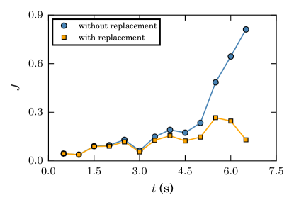
Figure 14: (Color on-line only) The contagion stress $J$ as a function of time $t$ in seconds (see text for details). The rounded symbols (in blue color) correspond to the $J$ values computed from a crowd of $N=131$ individuals and a sampling procedure “without replacement” (see Table 1 for details). The squared symbols correspond to the $J$ values computed from the same crowd, but following a sampling procedure “with replacement”. The mean stress for $0.5\,\mathrm{s}\leq t\leq 4\,\mathrm{s}$ is $J=0.1\pm 0.055$.

The $J$ estimates exhibited in Fig. 14 are not completely stationary along the interval $0.5\,\mathrm{s}\leq t\leq 4\,\mathrm{s}$. However, the increasing slope is not relevant for a first order approach. The mean value for the effective stress along this interval is $J=0.1\pm 0.055$.

References

- Volchenkov and Sharoff (2001) D. Volchenkov and S. Sharoff, in The Sciences of Complexity: From Mathematics to Technology to a Sustainable World, Vol. CD-ROM, edited by P. Blanchard, R. Lima, L. Streit, and R. V. Mendes (ZiF - Center for Interdisciplinary Research, 2001).
- Zhao et al. (2014) H. Zhao, J. Jiang, R. Xu, and Y. Ye, Mathematical Problems in Engineering 2014, 608315 (2014).
- Fu et al. (2014) L. Fu, W. Song, W. Lv, and S. Lo, Physica A: Statistical Mechanics and its Applications 405, 380 (2014).
- Fu et al. (2016) L. Fu, W. Song, W. Lv, X. Liu, and S. Lo, Simulation Modelling Practice and Theory 60, 1 (2016).
- Chen et al. (2015) G. Chen, H. Shen, G. Chen, T. Ye, X. Tang, and N. Kerr, Physica A: Statistical Mechanics and its Applications 417, 345 (2015).
- Ta et al. (2017) X.-H. Ta, B. Gaudou, D. Longin, and T. Ho, Informatica 41, 169 (2017).
- Pelechano et al. (2007) N. Pelechano, J.Allbeck, and N. Badler, Proceedings of the 2007 ACM SIGGRAPH/Eurographics Symposium on Computer Animation , 99 (2007).
- Nicolas et al. (2016) A. Nicolas, S. Bouzat, and M. N. Kuperman, Phys. Rev. E 94, 022313 (2016).
- Helbing et al. (2000) D. Helbing, I. Farkas, and T. Vicsek, Nature 407, 487 (2000).
- Helbing and Molnár (1995) D. Helbing and P. Molnár, Physical Review E 51, 4282 (1995).
- Frank and Dorso (2011) G. Frank and C. Dorso, Physica A 390, 2135 (2011).
- Parisi and Dorso (2005) D. Parisi and C. Dorso, Physica A 354, 606 (2005).
- Cornes et al. (2017) F. Cornes, G. Frank, and C. Dorso, Physica A: Statistical Mechanics and its Applications 484, 282 (2017).
- Michielsen and Raedt (2001) K. Michielsen and H. D. Raedt, Physics Reports 347, 461 (2001).
- (15) Rasband, W.S., ImageJ, U. S. National Institutes of Health, Bethesda, Maryland, USA, https://imagej.nih.gov/ij/, 1997-2016, .
- Frank and Dorso (2015) G. Frank and C. Dorso, International Journal of Modern Physics C 26, 1 (2015).
- Sticco et al. (2017) I. M. Sticco, F. E. Cornes, G. A. Frank, and C. O. Dorso, Phys. Rev. E 96, 052303 (2017).
- Plimpton (1995) S. Plimpton, Journal of Computational Physics 117, 1 (1995).