In-situ soil parametrization from multi-layer moisture data

Abstract

Inversion methodology has been used to obtain, from multi-layer soil probes records, a complete soil parametrisation, namely water retention curve, unsaturated conductivity curve and bulk density at 4 depths. The approach integrates water dynamics, hysteresis and the effect of bulk density on conductivity to extract soil parameters required from most simulation models. The method is applied to sub-sets of data collection, allowing to understand that not every data-sets contains the information required for method convergence. A comparison with experimental bulk-density values show that inversion could give information even with a better adherence to model, as it considers the effect of roots and skeleton. The method may be applied to any type of multi-layer water content probes giving the opportunity to enrich soil parameter availability and reliability.

1-University of Bologna, viale Fanin,44, 40127 Bologna, Italy
2-University of L’Aquila, via Vetoio, 67100 Coppito, L’Aquila, Italy
* corresponding author: giuliano.vitali@unibo.it

keywords - inverse problem, soil hydrology, soil structure

Introduction

Hydrological characterization of soils is a routine laboratory activity, and parameter values seem to suffice the needs of most soil-based model used in hydrology, agro-forestry, ecology, etc., whose complexity induces users to adopt a simplistic view of soil, referencing to standard soils or pedofunctions, in the belief of a low sensitivity on soil parametrization.

Soil is a complex system as well and, though the major lines of its hydrological behavior have been drawn, there are features not fully captured from math formalism, which are so forth not jet included in modeling.

In a porous system, water dynamics is ruled by Darcy-Buckingham law, where the driving variable is soil water potential (SWP,$\psi$). Such a variable, fundamental in controlling organism accessibility to water, is more difficult to measure than Soil Water Content (SWC,$\theta$). This is the reason why it is fundamental to know the relation between $\theta$ and $\psi$, the Water Retention Curve (WRC), long investigated in the domain of hydrology and soil physics. WRC has been interpreted from a wide series of functions [15], which often fail to represent the two faces of a soil, micro-and macro-porosity, the latter being related to structure (aggregation), which in turn depends on clay and organic matter content.

Sampling a soil always means altering its structure. Most of WRCs are obtained in laboratory by a drying process, generating parameters that hardly represent the original system, also explaining why soil hydrology models are hard to be calibrated ([3]).

These are the reasons why in-situ soil parametrization represents a fundamental task. Unfortunately in-situ methods to evaluate physical and hydrological parameters are complex, time expensive and with large errors[4] therefore a growing number of research have been oriented to inverse methods ([14]), aimed at obtaining the values of the parameters of a model the investigator nesting solution in a “non-linear fitting” methodology ([12]).

The objective of the present study is to identify parameters of constitutive relations (WRC and UWC) inverting a soil water dynamics model including bulk density variability along depth, and dependence of saturated conductivity on bulk density (see e.g. [11]).

Methodology has been developed to be fed by any soil multi-layer probes (recording SWC or surrogate variable at different depths), which allows to collect a long history of data.

In this paper we first describe the experimental setup from which the data has been described, the model used to interpret collected data, the inversion methodologies, the parameters obtained and a comparison with experimental bulk density values.

Materials and Methods

Data Records

SWC records come from an experimental site used for a study on hypogean fungi (truffle) near Bologna (Italy, location Saiarino, Lat.$44{{}^{\circ}}37\text{\textquoteright}N$, Lon.$11{{}^{\circ}}49\text{\textquoteright}E$, $5m$ asl), with a mediterranean sub-humid climate (sub-continental temperate, after Koppen) with c.ca $700mm$ precipitation, and mean air temperature $13{{}^{\circ}}C$. The site is located in the basin of Po valley, with an alluvial soil classified as aquic ustochrept, coarse loamy, mixed, thermic (USDA Soil Taxonomy - other parameters are available at http://geo.regione.emilia-romagna.it/cartpedo/). The site is on the banks of a land-reclamation channel, where different natural contexts may be found. In prior investigations 4 plots (P1..P4) have been chosen, and found to have slightly different physical parameters (Table 1), [6].

plot	texture		BD
	Sand	Clay	$g/cm^{3}$
P1	50-60	< 12	1.15-1.25
P2	30-40	18-25	1.45-1.60
P3	30-40	18-25	1.45-1.60
P4	30-40	18-25	1.00-1.15

Table 1: Physical characterization of the experimental plots from former observations.

The 4 plots have been delimited and split to have a rain-fed and an irrigated treatment: water has been supplied on July and August at intervals of 14 days in 2012 and 7 days in 2013, with 20 mm of water (dry-weeks only).

DM400 probes (by DFM Software - ZA, [1, 7], equipped with $4$ soil temperature and electric capacity sensors recording data at the depth of 10, 20, 30 and 40 cm, have been set on every irrigated sub-plots, and on rain-fed sub-plots of P1,P3. Hourly data have been recorded from spring 2012 to fall 2013.

Though the probes already return pre-calibrated SWC values, referred to as $\theta_{DFM}$, they have been re-calibrated in laboratory so as to correct SWCs by Soil Temperature ($Ts$) and bulk density ($\rho_{aps}$):

$$\theta=f(\theta_{DFM},T_{s},\rho_{aps})$$ (1)

Calibration procedure and relative results are described in Appendix A.

The Model

Soil water dynamics around probes is assumed to be 1-D so that the Darcy-Buckingham can be written in the form:

$$q=K(\theta)\cdot(1-\partial_{z}\psi_{t})$$ (2)

where $q$ is water flux, $K$ the water conductivity, and $\psi_{t}$ the total water potential ($\psi_{t}=\psi_{g}+\psi_{m}=z+\psi_{m}$ , being $\psi_{g}$ the gravitational potential, and $\psi_{m}$ the matrix potential). The equation can be solved combining it to the mass-conservation law, $\theta_{t}=q_{z}$ (generating the Richard’s law), defining proper Initial and Boundary Conditions, and adopting valid expressions for the Water Retention Curve (WRC ,$\psi(\theta)$ ), and for the Unsaturated Conductivity Curve (UCC $K(\theta)$ ). In this study the three-parameter van Genuchten ([13]) function is adopted:

$$\psi=\frac{(S^{n/(1-n)}-1)^{(1/n)}}{a}\quad;\quad 0\leq S\leq 1\quad,\quad n>1\quad,\quad a>0$$ (3)

where $n,a$ are two shape factors, while $S$ is saturation: $S=(\theta\text{\textendash}\theta_{R})/(\theta_{S}\text{\textendash}\theta_{R})$, where $\theta_{R}$ is residual water content and $\theta_{S}$ is the saturated SWC: $\theta_{S}=1\text{\textendash}\rho_{aps}/\rho_{S}$ ($\rho_{aps}$ being the bulk density and $\rho_{S}$ the real density, for non-organic soils assumed approximately $2.7g/cm^{3}$).

The model also includes hysteresis, which was accounted following the approach described in [5] where drying and wetting WRCs are respectively characterized by the shape factors $a_{d}$ and $a_{w}$ with $a_{d\>}\leq\>a_{w}$ .

The UCC is the one obtained coupling van Genuchten’s WRC to Mualem’s model ([8]) :

$$K=K_{S}\cdot S^{b}\cdot[1-(1-S^{1/m})^{m}]^{2};$$ (4)

commonly adopted with $m=1-1/n$, where $b$ is a shape factor.

To include the effect of soil structure on saturated conductivity, $K_{S}$ is assumed to be linearly related to bulk density, as suggested by results of [11] and [10]:

$$K_{S}=K_{\mu}+c\cdot(\rho_{\mu}-\rho_{aps})\quad,\quad\rho_{\mu}\succeq\rho_{aps}$$ (5)

where $K_{\mu}$ is the value of saturated conductivity for the compact soil (maximum bulk density:$\rho_{\mu}$), and $c$ is a proportionality coefficient depending on soil compaction.

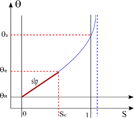
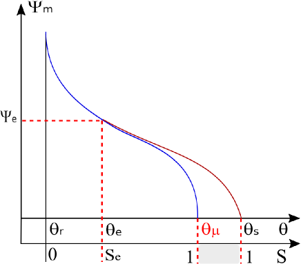
To include macro-porosity effect on WRC, instead of considering bi-modality, we adopt a stretching technique. Starting from the air-entry potential, $\psi_{e}=1/a$, a corresponding SWC value can be obtained $\theta_{e}=(\theta_{\mu}-\theta_{R})\cdot S_{e}+\theta_{R}$ , being a saturation value $S_{e}=S(\psi_{e},a,n)=2^{(1-n)/n}$, and where $\theta_{\mu}$ is the saturation SWC for a compact soil: $\theta_{\mu}=(1-\rho_{\mu}/\rho_{S})$. So forth we can define the slope that relates SWC and saturation in the low-saturation branch of WRC, $slp=(\theta_{e}-\theta_{R})/S_{e}$, from which a trend for the higher SWC values is derived: $\theta=\theta_{R}+slp\cdot erf^{-1}[S\cdot A]$, where the coefficient $A=erf[(\theta_{S}-\theta_{R})/slp]$ is used to force $\theta=\theta_{S}$ at $S=1$. The stretching scheme is represented in Figure 1.

Figure 1: Stretching scheme adopted to include macro-porosity in WRC

We finally assume that both WRC and UCC have the same parameters for the whole profile, while bulk density is changing along depth. Calibration function is also included in inversion procedure.

Inversion scheme

The solution scheme (see Appendix B) has been integrated into a standard parameter fitting procedure to compute expected value of SWC $\bar{\theta}$ at $20cm$ and $30cm$ depth. Though a huge number of collected data (> 10,000 per probe), the procedure requires that a change in $\theta$ values occurs simultaneously at every depth:

rule-a: $\theta_{DFM}(t,z)\neq\theta_{DFM}(t+\delta t,z)\>;\>z=10,20,30,40$.

a constraint which reduces considerably the number of valid data. Moreover, [9] suggests that to ensure that data contains the required information, their size should be sensitively greater than the number of parameters: $n_{data}\geq 2\cdot n_{parameters}+1$, therefore fitting has been operated on subsets with $n_{data}=30$ valid data.

The fitting techniques adopted in this study owns to a diffused class of inversion techniques based on Jacobian matrix: the Trust-Region-Reflective Algorithm [2] which is similar to the well known Levenberg-Marquard method, but it also includes parameter ranges. Minimum and maximum values of parameters are reported in table 2, together with the initial value.

	$\rho_{aps}$	$\theta_{R}$	$a_{d}$	$a_{w}$	$n$	$K\mu$	$c$	$b$
min	0.9	0	0.01	0.01	1	$10^{-4}$	0.3	5
max	1.8	0.1	0.05	0.25	4	$100$	3.0	20
ini	1.3	0.01	0.02	0.03	2	$1.0$	1.0	10

Table 2: Minimum, maximum and initial value of parameters used in inversion procedures

Methods of this class are quite sensitive to initial parameter guess ([12]), making the algorithm to be trapped in regions of parameter space with local minims. Nonetheless it is also true that data selected do not guarantee to own the information required to parameter identification: even models with few parameters could reach a complexity making the parameter search prohibitive [3].

To the scope a rule has been introduced to reject parameter-set where each of them differs from initial and extreme values:

rule-b: $|pi-p_{ini}|>\delta\cdot p_{ini}\quad OR\quad|pi-p_{min}|>\delta\cdot p_{ini}\quad OR\quad|pi-p_{max}|>\delta\cdot p_{ini}$

The set of parameters collected by data subsets have been finally tested for normality by Jarque-Bera test, after cutting the edges by different percentiles values. The considered window were $2-98_{ile}$, $5-95_{ile}$ and $10-90_{ile}$. Finally a comparison between parameter population have been performed by a Principal Component Analysis (PCA) to assess if the soil of the 4 plots are really different.

Comparison

to experimental values of parameters have been only performed for bulk density, which have been obtained in the field with the classical core method, with samples taken horizontally from a ditch (about 50cm diameter, 50cm depth) excavated inside each of the 4 main plots, by steel cylinders of $100cm^{3}$ , with 2 replicates for each depth.

Code

has been developed in Matlab (R2011b, The Mathworks, Inc.). For the NLF we used the embedded procedure sqcurvefit, with the (default) ’trust-region-reflective’ algorith: optimset(’TolFun’,1e-6,’TolX’,1e-5, ’Algorithm’,’trust-region-reflective’). Jarque-Bera test and PCA are also embedded in Matlab by the functions jbtest and princomp functions respectively.

Results

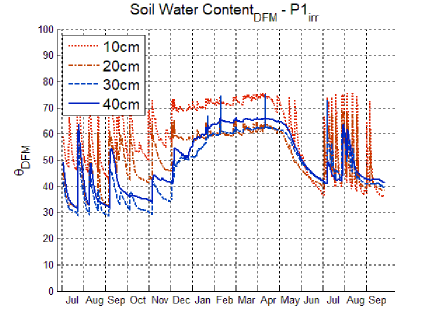
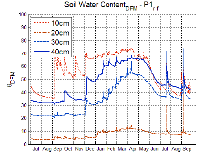
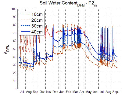
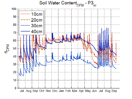
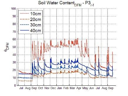
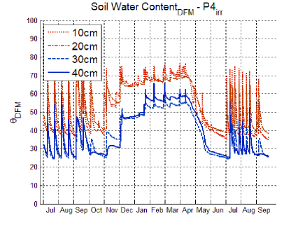
Hourly records of SWC ( $\theta_{DFM}$) for the 6 plots (4 irrigated+2 r-f sub-plots) are shown in 2 where a marked seasonal trends of soil moisture is visible at every depths.

Irrigated plots are easily recognizable from regular peaks in July an August, which rapidly decrease because of redistribution characterizing high conductive soils.

Figure 2: DFM’s SWC records for the 6 plots

Inversion results are shown in tables 3,4, and5. Table 3 reports the number of data-sets obtained for each plot by rule-a used for inversion ($n_{pre}$), the number of subsets passing rule-b and staying within the 3 percentile window considered, together with the relative J-B test response.

plot	$n_{pre}$		$n_{pos}$	$J-B$		$n_{pos}$	$J-B$		$n_{pos}$	$J-B$
			$2-98\%$			$5-95$			$10-90\%$
$1_{r-f}$	29		7	0		7	0		2	1
$1_{irr}$	100		17	1		5	1		2	1
$2_{irr}$	98		24	0		13	1		10	1
$3_{r-f}$	77		32	0		24	0		7	0
$3_{irr}$	141		38	0		30	0		13	1
$4_{irr}$	127		42	0		31	0		19	1

Table 3: Data sets available from data after filtering of rule-a and rule-b with different percentile windows

It can be seen that, as window becomes more selective, J-B test also results positive (normal distribution) but population reduces sensibly, therefore for the description of values (tables 4,5) the compromise window ($5-95$) has been chosen. Table 4 shows the average values of parameters. Columns 1 to 4 refer to bulk densities, with a value ranging from $1.08$ to $1.32$: largest values are reached in subsurface layers ($10-20cm$ and $20-30cm$).

About the parameters relative to WRC and UCC, despite of the result of J-B test, their values are quite close to one another, strengthening the idea that the plots have the same soil, and that any difference should be ascribed to spatial variability.

plot	$\rho_{aps-10}$	$\rho_{aps-20}$	$\rho_{aps-30}$	$\rho_{aps-40}$	$\theta_{R}$	$a_{d}$	$a_{w}$	$n$	$K_{\mu}$	$c$	$b$
	$(kg/m^{3})$	$(kg/m^{3})$	$(kg/m^{3})$	$(kg/m^{3})$	$(m^{3}/m^{3})$	$(-)$	$(-)$	$(-)$	$(cm/h)$	$(-)$	$(-)$
$1_{r-f}$	1.09	1.32	1.06	1.01	0.019	0.033	0.091	1.65	0.51	0.67	26.8
$1_{irr}$	1.10	1.13	1.13	1.10	0.027	0.028	0.053	1.78	0.50	0.60	23.1
$2_{irr}$	1.10	1.25	1.15	1.07	0.027	0.031	0.068	1.50	0.57	0.69	25.2
$3_{r-f}$	1.08	1.21	1.10	1.16	0.022	0.030	0.069	1.96	0.65	0.76	23.1
$3_{irr}$	1.19	1.13	1.30	1.07	0.041	0.031	0.077	1.54	0.61	0.73	25.0
$4_{irr}$	1.14	1.08	1.26	1.25	0.031	0.032	0.071	1.56	0.62	0.64	24.6

Table 4: Parameter averaged values obtained by the inversion technique

Standard deviations are reported in 5.

plot	$\rho_{aps-10}$	$\rho_{aps-20}$	$\rho_{aps-30}$	$\rho_{aps-40}$	$\theta_{R}$	$a_{d}$	$a_{w}$	$n$	$K_{\mu}$	$c$	$b$
	$(kg/m^{3})$	$(kg/m^{3})$	$(kg/m^{3})$	$(kg/m^{3})$	$(m^{3}/m^{3})$	$(-)$	$(-)$	$(-)$	$(cm/h)$	$(-)$	$(-)$
$1_{r-f}$	0.13	0.06	0.03	0.06	0.013	0.005	0.03	0.38	0.23	0.13	3.2
$1_{irr}$	0.05	0.07	0.04	0.07	0.017	0.005	0.03	0.22	0.22	0.19	5.0
$2_{irr}$	0.04	0.01	0.02	0.04	0.016	0.003	0.01	0.20	0.13	0.09	2.9
$3_{r-f}$	0.03	0.04	0.06	0.03	0.009	0.006	0.03	0.47	0.09	0.06	3.7
$3_{irr}$	0.06	0.03	0.02	0.02	0.017	0.001	0.01	0.07	0.04	0.03	1.5
$4_{irr}$	0.03	0.02	0.01	0.02	0.011	0.003	0.02	0.08	0.07	0.10	3.1

Table 5: Parameter standard deviation values obtained by the inversion technique

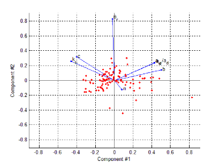
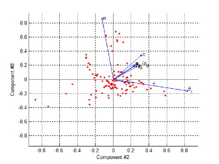
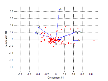
To corroborate the hypothesis of a common soil, a PCA has been performed on the last 7 parameters (bulk density has been excluded as it depends on depth also), using the 110 parameter sets. From PCA it resulted that the first principal component is responsible of $48.3$ of variability with an eigenvector (table 6) ascribing such variability to the main shape factors of WRC ($a_{d}$ and $n$). Component #2 and #3 are responsible of respectively $16.8$ and $15.7$; the other 4 components are of minor importance.

Compaction factor $c$, influenceing conductivity, is relevant in component #3, #5 and #6, whereas $a_{w}/a_{d}$ related to hysteresis, mainly affects #4, to which is ascribed $8.6\%$ of global variance.

component	var	$\theta_{R}$	$a_{d}$	$a_{w}/a_{d}$	$n$	$K_{\mu}$	$c$	$b$
1	48.3	-0.019	0.829	-0.162	0.511	-0.067	-0.050	-0.134
2	16.8	0.431	0.235	0.187	-0.250	0.779	0.086	-0.215
3	15.7	0.425	0.239	0.202	-0.469	-0.5091	-0.452	-0.193
4	8.6	0.083	-0.124	0.863	0.475	-0.049	-0.054	0.033
5	5.2	-0.462	0.259	0.180	-0.247	0.264	-0.495	0.558
6	3.2	-0.402	0.315	0.343	-0.411	-0.190	0.633	-0.121
7	2.2	0.501	0.139	-0.040	-0.004	-0.144	0.369	0.756

Table 6: Results of the PCA analysis in terms of component effects on variances and eigenvectors composition; larger values are put in bold

A plot of the three main components is drawn in figure 3 show there is no evidence of clustering.

Figure 3: Plot of the cases (red points) and of main 2 components

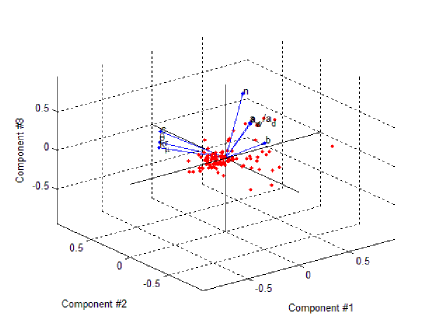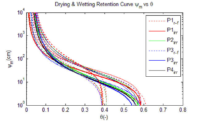
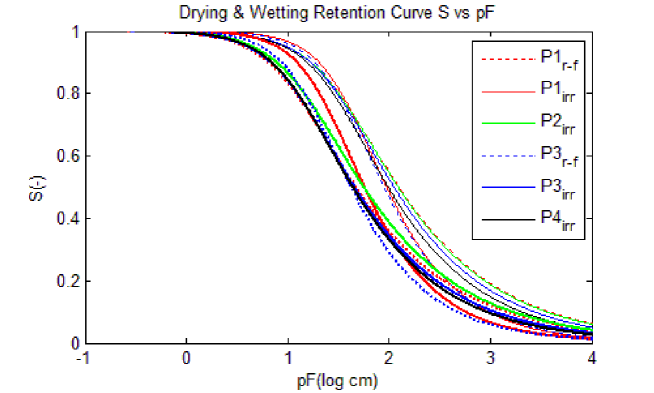
Figure 4 shows the WRCs for the 6 cases.

Figure 4: WRCs for the 6 plots: continuous lines are for irrigated plots, dashed lines for rain-fed plots. Bold lines are wetting curves.In the top graph, both un-stretched and stretched (for top soil layer) WRCs are shown.

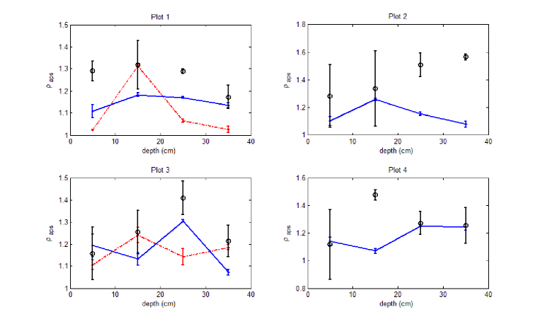
Experimental evaluation of bulk densities show high error bars of experimental values, due to operative difficulties intrinsic of the method, hard to be overcome in natural soils, due to roots and skeleton. Inverse problem solving, if from the one side seems to underestimate BD values, it may also confirm a typical problem of core method, soil compression due to dragging effect of the cylinder wall. Model also emphasizes bulk density differences along soil depth, most of times in agreement with those observed with core method, as represented in Figure 5.

Figure 5: Estimated and measured bulk densities (BD) for the 4 plots; plots 1,3 have rain-fed (red lines) and irrigated conditions, plots 2,4 only irrigated (blue lines). Circles represent measured data. Error bars stand for standard deviations.

Indirect validation of parameters have been performed using the SWP as a driving variable in a recently developed model to simulate mycelium growth in the same plots [6].

Conclusions

Inversion technique developed in this study, obtained by integration of a refined soil water dynamical model in a classical non-linear fitting method, is used to derive in-situ soil hydrological parameters from soil moisture multi-depth probe records. The features included, namely soil hysteresis, dependence of conductivity to bulk-density, and inclusion of calibration curve confirm that inversion procedures can give parameter with a validity both comparable to experimental methods, and adherent to a real-world soil system.

The analysis also confirms that convergence strongly depended on the size of available data records: in fact in general data can not guarantee to own the information required from problem inversion.

From PCA analysis emerges that the plots analyzed corresponds to the same soil, and that spatial variability affects the value of each of parameters used to represent the soil.

Finally, though the methodology gave prove of robustness, it is required to be assessed jet on a set of sufficiently different soils jet.

The method can be extended to a wide class of probes, including the cheapest ones today wide-spreading under the push of Internet of Things (IoT), which rapidly increase the number of highly connected low cost specialized devices placed everywhere, and that will give the opportunity to enrich enormously the knowledge about soils and its reliability.

Credits

The manuscript has been edited by Lyx ver.2.1.1, using as Document Class the Article (Standard Class), references have been managed by Mendeley ver.1.17.13 and JabRef 3.8.2.

Appendix A - Calibration

DFM probe calibration DFM probes estimate soil water content on the basis of dielectric properties of wet soil. As they are mostly used for a comparative use, within a water scheduling framework, they come with a general purpose calibration which does not ensure a precise evaluation of water content for local soil. Nevertheless the several sensors DFM probes are equipped with (DFM400 has $4$ $10cm$-spaced sensors) can be assumed to have an identical behavior, therefore the calibration has been performed on one of them. To calibrate a sensor the DFM probe have been placed in a plastic cylinder ($diam=12cm$, $len=10cm$) so as to have a single sensor surrounded by soil with a known density and water content (added to the soil after it be oven-dried). The cylinder has a bottom with a central hole for the probe drilled to drain excess water, whereas is open above and hanged to a scale, allowing a gravitational determination of water content. The cylinder is formerly filled with dry soil, then saturated and left drying in a warm room. The trial has been repeated with different soils and different density, allowing to obtain the following calibration expression:

$$\theta=[0.01\>\theta_{DFM}\>(1+0.0018\>(20-Ts))\text{\textendash}a_{1}\text{\textendash}a_{2}\rho_{aps}^{m}]/[a_{3}+a_{4}\rho_{aps}^{m}]^{1/m}$$ (6)

where $\theta_{DFM}$ is the read value, Ts is soil temperature and $\rho_{aps}$ the bulk density. Parameters, estimated by a trial and error procedure, are: $a_{1}=46.2$,$a_{2}=46.7$, $a_{3}=-51.8$ , $a_{4}=53.1$, $m=0.2=1/5$ ,with $R^{2}=0.993$.

Appendix B - Numerical scheme

The equations described above have been discretized as follows below to get the estimated SWC $\bar{\theta}$ in the intermediate nodes ($j=2,3$; $20,30cm$):

$$\overline{\theta}_{i,j} = \frac{[K_{j-1}+K_{j}]}{2}\cdot\frac{[\psi_{i,j-1}-\psi_{i,j}-dz]}{dz}\cdot dt-\frac{[K_{j}+K_{j+1}]}{2}\cdot\frac{[\psi_{i,j}-\psi_{i,j+1}-dz]}{dz}\cdot dt$$

$$K_{j} = Ks_{j}\cdot S_{i,j}^{b}(1-(1-S_{i,j}^{1/m})^{m})^{2}$$

$$Ks_{j} = K_{\mu}\cdot(1+c\cdot[\rho_{aps-j}-1])$$

$$\psi_{i,j} = (S_{i,j}{}^{n/(1-n)}-1)^{(1/n)}/a$$

To include hysteresis procedure, the parameter $a$ is assigned one of two different values, depending on sign of water content change:

$$a= \begin{cases}a_{w}\Leftarrow\theta_{DFM;i}<\theta_{DFM;i+1}\\ a_{d}\Leftarrow\theta_{DFM;i}>\theta_{DFM;i+1}\end{cases}$$

and saturation $S$ is computed by the stretching function for the given SWC:

$$S_{i,j} = erf((\theta_{i,j}-\theta_{R})/slp)/A$$

$$\theta_{i,j} = f[\theta_{DFM;i,j},T_{S-i,j},\rho_{aps-j}]$$

$$A = erf[(\theta_{S-j}-\theta_{R})/slp]$$

$$slp = (\theta_{e-j}-\theta_{R})/S_{e}$$

$$\theta_{e-j} = (\theta_{\mu}-\theta_{R})\cdot S_{e}+\theta_{R}$$

$$\theta_{\mu} = (1-\rho_{\mu}/\rho_{s})$$

$$\theta_{S-j} = (1-\rho_{aps-j}/\rho_{s})$$

$$\rho_{aps-j} = \rho_{\mu}-\delta\rho_{j}$$

$$S_{e} = 2^{(1-n)/n}$$

where $\delta\rho_{1..4}$ , $\theta_{R}$, $a_{d}$ ,$a_{w}$, $n$, $K_{\mu}$, $c$ ,$b$, are the fitted parameters.

Appendix C - Parameter Distributions

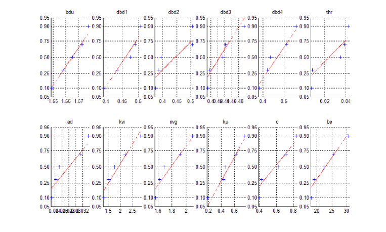
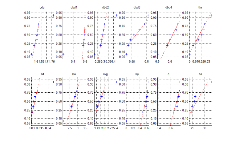
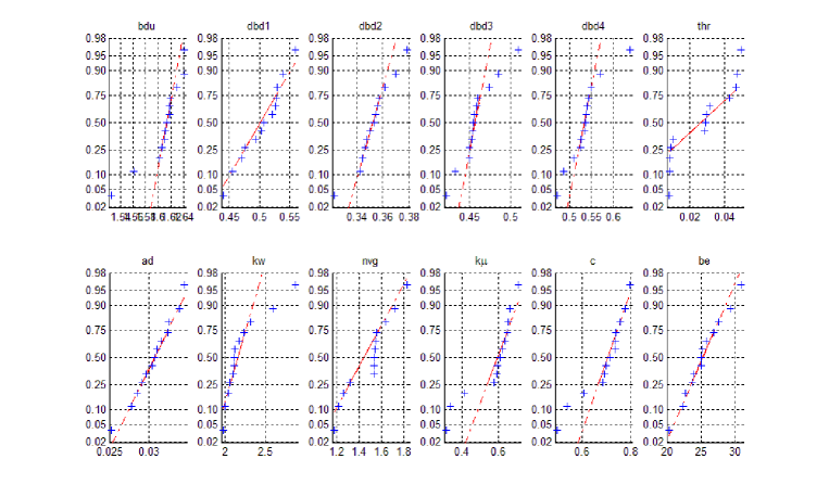
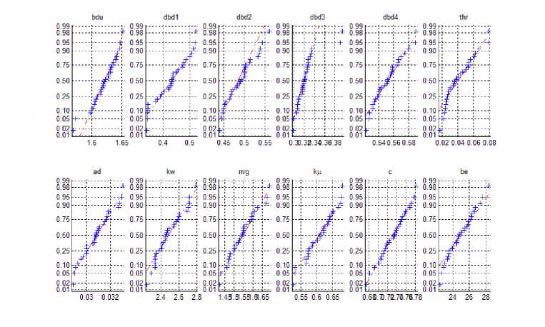
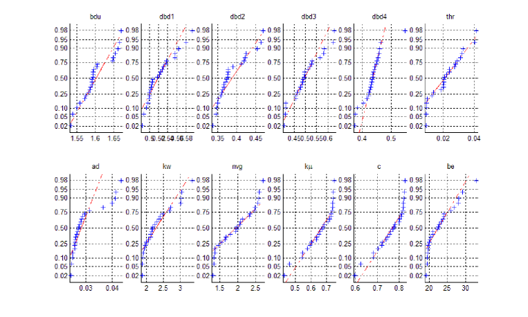
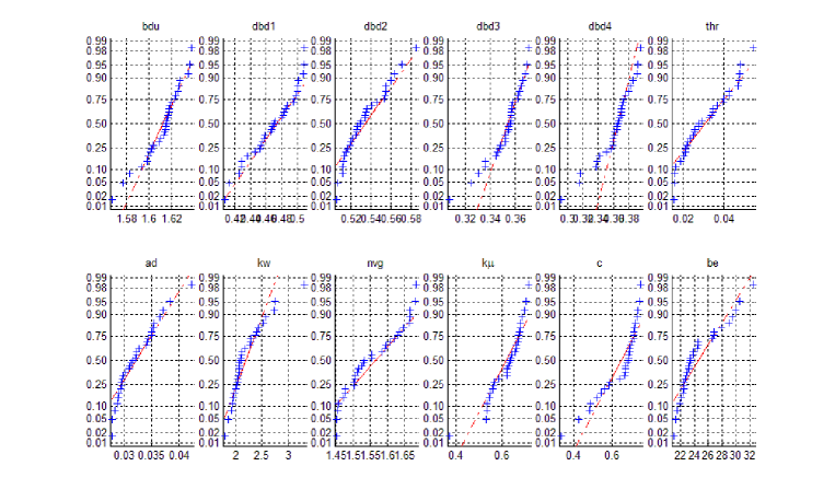
In the following figures, are the values of parameter obtained from model inversion for the 6 plots.

Figure 6: Parameter values for Plot 1 - irrigated

Figure 7: Parameter values for Plot 1 - rainf-fed

Figure 8: Parameter values for Plot 2 - irrigated

Figure 9: Parameter values for Plot 3 - irrigated

Figure 10: Parameter values for Plot 3 - rain-fed

Figure 11: Parameter values for -Plot 4 - irrigated

.

References

- [1] AAVV_DFM, The DFM continuous logging soil moisture probe - Functional specifications, Tech. report, 2010.
- [2] Andrew R. Conn, Nicholas I. M. Gould, and Philippe L. Toint, Trust-region methods, Society for Industrial and Applied Mathematics, 2000.
- [3] Qingyun Duan, Soroosh Sorooshian, and Vijai Gupta, Effective and efficient global optimization for conceptual rainfall-runoff models, Water Resources Research 28 (1992), no. 4, 1015–1031.
- [4] Wolfgang Durner and Kai Lipsius, Determining Soil Hydraulic Properties, Encyclopedia of Hydrological Sciences, John Wiley & Sons, Ltd, Chichester, UK, oct 2005.
- [5] S. Elmaloglou and E. Diamantopoulos, The effect of hysteresis on three-dimensional transient water flow during surface trickle irrigation, Irrigation and Drainage 57 (2008), no. 1, 57–70.
- [6] Mirco Iotti, Pamela Leonardi, Giuliano Vitali, and Alessandra Zambonelli, Effect of summer soil moisture and temperature on the vertical distribution of Tuber magnatum mycelium in soil, submitted (2018).
- [7] Nokhwezi Mjanyelwa, Zaid A. Bello, Willnerie Greaves, and Leon D. van Rensburg, Precision and accuracy of DFM soil water capacitance probes to measure temperature, Computers and Electronics in Agriculture 125 (2016), no. C, 125–128.
- [8] Yechezkel Mualem, A new model for predicting the hydraulic conductivity of unsaturated porous media, Water Resources Research 12 (1976), no. 3, 513–522.
- [9] J. A. Nelder and R. Mead, A Simplex Method for Function Minimization, The Computer Journal 7 (1965), no. 4, 308–313.
- [10] J.A. Osunbitan, D.J. Oyedele, and K.O. Adekalu, Tillage effects on bulk density, hydraulic conductivity and strength of a loamy sand soil in southwestern Nigeria, Soil and Tillage Research 82 (2005), no. 1, 57–64.
- [11] C.F. Shaykewitch, Hydraulic Properties of Disturbed and Undisturbed Soils, Can.J.Soil Sci. 50 (1970), 430–437.
- [12] Albert Tarantola, Inverse Problem Theory and Methods for Model Parameter Estimatio, SIAM-Society for Industrial and Applied Mathematics, Phyladelphia, 2005.
- [13] M. Th. van Genuchten, A Closed-form Equation for Predicting the Hydraulic Conductivity of Unsaturated Soils1, Soil Science Society of America Journal 44 (1980), no. 5, 892.
- [14] Jasper A. Vrugt, Philip H. Stauffer, Th. Wohling, Bruce A. Robinson, and Velimir V. Vesselinov, Inverse Modeling of Subsurface Flow and Transport Properties: A Review with New Developments, Vadose Zone Journal 7 (2008), no. 2, 843.
- [15] M. Wijaya and E.C. Leong, Equation for unimodal and bimodal soil–water characteristic curves, Soils and Foundations 56 (2016), no. 2, 291–300.