On the Convergence of the SINDy Algorithm

Abstract

One way to understand time-series data is to identify the underlying dynamical system which generates it. This task can be done by selecting an appropriate model and a set of parameters which best fits the dynamics while providing the simplest representation (i.e. the smallest amount of terms). One such approach is the sparse identification of nonlinear dynamics framework [6] which uses a sparsity-promoting algorithm that iterates between a partial least-squares fit and a thresholding (sparsity-promoting) step. In this work, we provide some theoretical results on the behavior and convergence of the algorithm proposed in [6]. In particular, we prove that the algorithm approximates local minimizers of an unconstrained $\ell^{0}$-penalized least-squares problem. From this, we provide sufficient conditions for general convergence, rate of convergence, and conditions for one-step recovery. Examples illustrate that the rates of convergence are sharp. In addition, our results extend to other algorithms related to the algorithm in [6], and provide theoretical verification to several observed phenomena.

1 Introduction

Dynamic model identification arises in a variety of fields, where one would like to learn the underlying equations governing the evolution of some given time-series data $u(t)$. This is often done by learning a first-order differential equation $\dot{u}=f(u)$ which provides a reasonable model for the dynamics. The function $f$ is unknown and must be learned from the data. Some applications including, weather modeling and prediction, development and design of aircraft, modeling the spread of disease over time, trend predictions, etc.

Several analytical and numerical approaches have been developed to solve various model identification problems. One important contribution to model identification is [4, 23], where the authors introduced a symbolic regression algorithm to determine underlying physical equations, like equations of motion or energies, from data. The key idea is to learn the governing equation directly from the data by fitting the derivatives with candidate functions while balancing between accuracy and parsimony. In [6], the authors proposed the sparse identification of nonlinear dynamics (SINDy) algorithm, which computes sparse solutions to linear systems related to model identification and parameter estimation. The main idea is to convert the (nonlinear) model identification problem to a linear system:

$$Ax=b,$$ (1.1)

where the matrix $A\in\mathbb{R}^{m\times n}$ is a data-driven dictionary whose columns are (nonlinear) candidate functions of the given data $u$, the unknown vector $x\in\mathbb{R}^{n}$ represents the coefficients of the selected terms in the governing equation $f$, and the vector $b\in\mathbb{R}^{m}$ is an approximation to the first-order time derivative $\dot{u}$. In this method, the number of candidate functions are fixed, and thus one assumes that the set of candidate functions is sufficiently large to capture the nonlinear dynamics present in the data. In order to select an accurate model (from the set of candidate functions) which does not overfit the data, the authors of [6] proposed a sparsity-promoting algorithm. In particular, a sparse vector $x$ which approximately solves Equation (1.1) is generated by the following iterative scheme:

$$S^{k} =\{1\leq j\leq n:|x_{j}^{k}|\geq\lambda\},$$ (1.2a)

$$x^{k+1} =\underset{x\in\mathbb{R}^{n}:\ {\rm supp}(x)\subseteq S^{k}}{\mathrm{argmin}}\|Ax-b\|_{2},$$ (1.2b)

where $\lambda>0$ is a thresholding parameter and ${\rm supp}(x)$ is the support set of $x$. In practice, it was observed that the algorithm converged within a few steps and produced an appropriate sparse approximation to Equation (1.1). These observations are quantified in our work.

There are several approaches which leverage sparse approximations for model identification. In [9], the authors combined the SINDy framework with model predictive control to solve model identification problems given noisy data. The resulting algorithm is able to control nonlinear systems and identify models in real-time. In [13], the authors introduced information criteria to the SINDy framework, where they selected the optimal model (with respect to the chosen information criteria) over various values of the thresholding parameter. Other approaches have been developed based on the SINDy framework, including: SINDy for rational governing equations [12], SINDy with control [7], and SINDy for abrupt changes [15].

In [19], a sparse regression approach for identifying dynamical systems via the weak form was proposed. The authors used the following constrained minimization problem:

$$\min_{x}\|x\|_{0}\quad\text{subject to }\|Ax-b\|_{2}\leq\sigma,$$

where the dictionary matrix $A$ is formulated using an integrated set of candidate functions. In [20], several sampling strategies were developed for learning dynamical equations from high-dimensional data. It was proven analytically and verified numerically that under certain conditions, the underlying equation can be recovered exactly from the following constrained minimization problem, even when the data is under-sampled:

$$\min_{x}\|x\|_{1}\quad\text{subject to }\|Ax-b\|_{2}\leq\sigma,$$

where the dictionary matrix $A$ consists of second-order Legendre polynomials applied to the data. In [21], the authors developed an algorithm for learning dynamics from multiple time-series data, whose governing equations have the same form but different (unknown) parameters. The authors provided convergence guarantees for their group-sparse hard thresholding pursuit algorithm; in particular, one can recover the dynamics when the data-drive dictionary is coercive. In [26], the authors provided conditions for exact recovery of dynamics from highly corrupted data generated by Lorenz-like systems. To separate the corrupted data from the uncorrupt points, they solve the minimization problem:

$$\min_{x,\eta}\|\eta\|_{2,1}\quad\text{subject to }Ax+\eta=b\text{ and $x$ is sparse},$$

where the residual $\eta:=b-Ax$ is the variable representing the (unknown) corrupted locations. When the data is a function of both time and space, i.e. $u=u(t,y)$ for some spatial variable $y$, the dictionary can incorporate spatial derivatives [18, 17]. In [18], an unconstrained $\ell^{1}$-regularized least-squares problem (LASSO [25]) with a dictionary build from nonlinear functions of the data and its spatial partial derivatives was used to discover PDE from data. In [17], the authors proposed an adaptive SINDy algorithm for discovering PDE, which iteratively applies ridge regression with hard thresholding. Additional approaches for model identification can be found in [24, 5, 8, 11, 14, 10, 16, 22].

The sparse model identification approaches include a sparsity-promoting substep, typically through various thresholding operations. In particular, the SINDy algorithm, i.e. Equation (1.2), alternates between a reduced least-squares problem and a thresholding step. This is related to, but differs from, the iterative thresholding methods widely used in compressive sensing. To find a sparse representation of $x$ in Problem (1.1), it is natural to solve the $\ell^{0}$-minimization problems, where the $\ell^{0}$-penalty of a vector measures the number of its nonzero elements. In [3, 1, 2], the authors provided iterative schemes to solve the unconstrained and constrained $\ell^{0}$-regularized problems:

$$\min_{x}\|Ax-b\|_{2}^{2}+\lambda^{2}\|x\|_{0},$$ (1.3)

$$\min_{x}\|Ax-b\|_{2}^{2}\quad\text{subject to }\|x\|_{0}\leq s,$$ (1.4)

respectively, where $\|A\|_{2}=1$. To solve Problem (1.3), one iterates:

$$x^{k+1}=H_{\lambda}(x^{k}+A^{T}(b-Ax^{k})),$$ (1.5)

where $H_{\lambda}$ is the hard thresholding operator defined component-wise by:

$$H_{\lambda}(x)_{j}:={\rm sgn}(x_{j})\max(|x_{j}|,\lambda).$$

To solve Problem (1.4), one iterates:

$$x^{k+1}=L_{s}(x^{k}+A^{T}(b-Ax^{k})),$$ (1.6)

where $L_{s}$ is a nonlinear operator that only retains $s$ elements of $x$ with the largest magnitude and sets the remaining $n-s$ elements to zero.

The authors of [3, 1, 2] also proved that the iterative algorithms defined by Equations (1.5) and (1.6) converge to the local minimizers of Problems (1.3) and (1.4), respectively, and derived theoretically the error bounds and convergence rates for the solutions obtained via Equation (1.5). In this work, we will show that the SINDy algorithm also finds local minimizers of Equation (1.3) and has similar theoretical guarantees.

1.1 Contribution

In this work, we show (in Section 2) that the SINDy algorithm proposed in [6] approximates the local minimizers of Problem (1.3). We provide sufficient conditions for convergence and bounds on rate of convergence. We also prove that the algorithm typically converges to a local minimizer rapidly (in a finite number of steps). Based on several examples, the rate of convergence is sharp. We also show that the convergence results can be adapted to other SINDy-based algorithms. In Section 3, we highlight some of the theoretical results by applying the algorithm from [6] to identify dynamical systems from noisy measurements.

2 Convergence Analysis

Before detailing the results, we briefly introduce some notations and conventions. For an integer $n\in\mathbb{N}$, let $[n]\subset\mathbb{N}$ be the set defined by: $[n]:=\{1,2,\cdots,n\}$. Let $A$ be a matrix in $\mathbb{R}^{m\times n}$, where $m\geq n$. If $A$ is injective (or equivalently if $A$ is full column rank, i.e. ${\rm rank}(A)=n$), then its pseudo-inverse $A^{\dagger}\in\mathbb{R}^{n\times m}$ is defined as $A^{\dagger}:=(A^{T}A)^{-1}A^{T}$. Let $x\in\mathbb{R}^{n}$ and define the support set of $x$ as the set of indices corresponding to its nonzero elements, i.e.,

$${\rm supp}(x):=\{j\in[n]:x_{j}\neq 0\}.$$

The $\ell^{0}$ penalty of $x$ measures the number of nonzero elements in the vector and is defined as:

$$\|x\|_{0}:={\rm card}({\rm supp}(x)).$$

The vector $x$ is called $s$-sparse if it has at most $s$ nonzero elements, thus $\|x\|_{0}\leq s$.

Given a set $S\subseteq[n]$, where $n\in\mathbb{N}$ is known from the context, define $\bar{S}:=[n]\backslash S$. For a matrix $A\in\mathbb{R}^{m\times n}$ and a set $S\subseteq[n]$, we denote by $A_{S}$ the submatrix of A in $\mathbb{R}^{m\times s}$ which consists of the columns of $A$ with indices $j\in S$, where $s={\rm card}(S)$. Similarly, for a vector $x=\begin{pmatrix}x_{1},x_{2},\cdots,x_{n}\end{pmatrix}^{T}$, let $x_{S}$ be the subvector of $x$ in $\mathbb{R}^{s}$ consisting of the elements of $x$ with indices $j\in S$, or the vector in $\mathbb{R}^{n}$ which coincides with $x$ on $S$ and is zero outside $S$:

$$(x_{S})_{j}=\begin{cases}x_{j}&\quad\text{if }j\in S,\\ 0&\quad\text{if }j\in\bar{S}.\end{cases}$$

The representation of $x_{S}$ should be clear within the context.

2.1 Algorithmic Convergence

Let $A\in\mathbb{R}^{m\times n}$ be a matrix with $m\geq n$ and ${\rm rank}(A)=n$, $x\in\mathbb{R}^{n}$ be the unknown signal, and $b\in\mathbb{R}^{m}$ be the observed data. The results presented here work for general $A$ satisfying these assumptions, but the specific application of interest is detailed in Section 3. The SINDy algorithm from [6] is:

$$x^{0} =A^{\dagger}b,$$ (2.1a)

$$S^{k} =\{j\in[n]:|x_{j}^{k}|\geq\lambda\},\quad k\geq 0,$$ (2.1b)

$$x^{k+1} =\underset{x\in\mathbb{R}^{n}:{\rm supp}(x)\subseteq S^{k}}{\mathrm{argmin}}\|Ax-b\|_{2}\quad k\geq 0.$$ (2.1c)

which is used to find a sparse approximation to the solution of $Ax=b$. The following theorem shows that the SINDy algorithm terminates in finite steps.

Theorem 2.1.

The iterative scheme defined by Equation (2.1) converges in at most $n$ steps.

Proof.

Let $x^{k}$ be the sequence generated by Equation (2.1). By Equation (2.1c) we have ${\rm supp}(x^{k+1})\subseteq S^{k}$, and from Equation (2.1b) we have $S^{k+1}\subseteq{\rm supp}(x^{k+1})$. Therefore, the sets $S^{k}$ are nested:

$$S^{k+1}\subseteq{\rm supp}(x^{k+1})\subseteq S^{k}.$$ (2.2)

Consider the following two cases. If there exists an integer $M\in\mathbb{N}$ such that $S^{M+1}=S^{M}$, then:

$$x^{M+2} =\underset{{\rm supp}(x)\subseteq S^{M+1}}{\mathrm{argmin}}\|Ax-b\|_{2}=\underset{{\rm supp}(x)\subseteq S^{M}}{\mathrm{argmin}}\|Ax-b\|_{2}=x^{M+1}.$$ (2.3)

Thus, $x^{k}=x^{M+1}$ for all $k\geq M+1$, and $S^{k}=S^{M}$ for all $k\geq M$. Since ${\rm card}(S^{k})\leq n$ for all $k\in\mathbb{N}$, we conclude that $M\leq n$, so that the scheme converges in at most $n$ steps.

On the other hand, if there does not exist an integer $M$ such that $S^{M+1}=S^{M}$ and $S^{M}\neq\emptyset$, then we have a sequence of strictly nested sets, i.e.,

$$S^{k+1}\subsetneq S^{k}\quad\text{for all }k\text{ such that }S^{k}\neq\emptyset.$$

Since ${\rm card}(S^{k})\leq n$ for all $k\in\mathbb{N}$, we must have $S^{k}=\emptyset$ for all $k>n$. Therefore, the scheme converges to the trivial solution within $n$ steps. ∎

Remark 2.2.

Equation (2.3) suggests that an appropriate stopping criterion for the scheme is that the sets are stationary, i.e. $S^{k}=S^{k-1}$.

Note that, since the support sets are nested, the scheme will converge in at most ${\rm card}(S^{0})$ steps. The following is an immediate consequence of Theorem 2.1.

Corollary 2.3.

The iterative scheme defined by Equation (2.1) converges to an $s$-sparse solution in at most ${\rm card}(S^{0})-s$ steps.

2.2 Convergence to the Local minimizers

In this section, we will show that the iterative scheme defined by Equation (2.1) produces a minimizing sequence for a non-convex objective associated with sparse approximations. This will lead to a clearer characterization of the fixed-points of the iterative scheme.

Without loss of generality, assume in addition that $\|A\|_{2}=1$. We first show that the scheme converges to a local minimizer of the following (non-convex) objective function:

$$F(x):=\|Ax-b\|_{2}^{2}+\lambda^{2}\|x\|_{0},\quad x\in\mathbb{R}^{n}.$$ (2.4)

Theorem 2.4.

The iterates $x^{k}$ generated by Equation (2.1) strictly decreases the objective function unless the iterates are stationary.

Proof.

Define the auxiliary variable:

$$y^{k}:=x^{k}_{S^{k}},\quad k\in\mathbb{N},$$ (2.5)

which plays the role of an intermediate approximation. In particular, we will relate $x^{k+1}$ and $y^{k}$.

Observe that Equation (2.1) emits several useful properties. First, we have shown in Equation (2.2) that $S^{k+1}\subseteq{\rm supp}(x^{k+1})\subseteq S^{k}$. Next, by Equation (2.1c), $x^{k+1}$ is the least-squares solution over the set $S^{k}$. By considering the derivative of $\|Ax-b\|_{2}^{2}$ with respect to $x$, we obtain that:

$$\left(A^{T}(Ax^{k+1}-b)\right)_{S^{k}}=0,$$ (2.6)

and the solution $x^{k+1}$ to the above equation satisfies $x^{k+1}_{S^{k}}=(A_{S^{k}})^{\dagger}b$. To relate $x^{k+1}$ and $y^{k}$, note that Equations (2.2) and (2.5) imply that:

$${\rm supp}(x^{k+1})\subseteq{\rm supp}(y^{k})=S^{k}\subseteq{\rm supp}(x^{k}).$$ (2.7)

By Equations (2.1c) and (2.7), we have:

$$\|Ax^{k+1}-b\|_{2}\leq\|Ay^{k}-b\|_{2},\quad\text{and}\quad\|x^{k+1}\|_{0}\leq\|y^{k}\|_{0},$$ (2.8)

respectively.

To show that the objective function decreases, we use the optimization transfer technique as in [3]. Define the surrogate function $G$ for $F$:

$$G(x,y):=\|Ax-b\|_{2}^{2}-\|A(x-y)\|_{2}^{2}+\|x-y\|_{2}^{2}+\lambda^{2}\|x\|_{0},\quad x\in\mathbb{R}^{n}.$$ (2.9)

Since $\|A\|_{2}=1$, the term $-\|A(x-y)\|_{2}^{2}+\|x-y\|_{2}^{2}$ is non-negative:

$$-\|A(x-y)\|_{2}^{2}+\|x-y\|_{2}^{2}\geq-\|A\|_{2}^{2}\|x-y\|_{2}^{2}+\|x-y\|_{2}^{2}=0,$$

and thus we have $G(x,y)\geq F(x)$ and $G(x,x)=F(x)$ for all $x,y\in\mathbb{R}^{n}$.

Define the matrix $B:=I-A^{T}A$. Since $A$ is injective (which is implied by ${\rm rank}(A)=n$) and $\|A\|_{2}=1$, we have that the eigenvalues of $B$ are in the interval $[0,1]$. Fixing the index $k\in\mathbb{N}$, from Equations (2.4) and (2.8)-(2.9), we have:

$$F(x^{k+1})=\|Ax^{k+1}-b\|_{2}^{2}+\lambda^{2}\|x^{k+1}\|_{0} \leq\|Ax^{k+1}-b\|_{2}^{2}+\lambda^{2}\|x^{k+1}\|_{0}+\|x^{k}-y^{k}\|_{B}^{2}$$

$$\leq\|Ay^{k}-b\|_{2}^{2}+\lambda^{2}\|y^{k}\|_{0}+\|x^{k}-y^{k}\|_{B}^{2}=G(y^{k},x^{k}).$$

It remains to show that $G(y^{k},x^{k})\leq G(x^{k},x^{k})$. By Equation (2.5), we have:

$$x^{k}-y^{k}=x^{k}-x^{k}_{S^{k}}=x^{k}_{{\rm supp}(x^{k})}-x^{k}_{S^{k}\cap{\rm supp}(x^{k})}=x^{k}_{\bar{S}^{k}\cap{\rm supp}(x^{k})},$$

where we included the intersection with ${\rm supp}(x^{k})$ to emphasize that the difference is zero outside of the support set of $x^{k}$. Thus, the difference with respect to the surrogate function simplifies to:

$$G(y^{k},x^{k})-G(x^{k},x^{k})$$

$$\quad=\|Ay^{k}-b\|_{2}^{2}-\|A(y^{k}-x^{k})\|_{2}^{2}+\|y^{k}-x^{k}\|_{2}^{2}+\lambda^{2}\|y^{k}\|_{0}-\|Ax^{k}-b\|_{2}^{2}-\lambda^{2}\|x^{k}\|_{0}$$

$$\quad=-2\langle b,Ay^{k}\rangle+2\langle Ay^{k},Ax^{k}\rangle-2\|Ax^{k}\|_{2}^{2}+2\langle b,Ax^{k}\rangle+\|x^{k}-y^{k}\|_{2}^{2}+\lambda^{2}\left(\|y^{k}\|_{0}-\|x^{k}\|_{0}\right)$$

$$\quad=-2\langle y^{k}-x^{k},A^{T}(b-Ax^{k})\rangle+\|x^{k}-y^{k}\|_{2}^{2}+\lambda^{2}\left(\|y^{k}\|_{0}-\|x^{k}\|_{0}\right)$$

$$\quad=-2\langle x^{k}_{\bar{S}^{k}\cap{\rm supp}(x^{k})},A^{T}(Ax^{k}-b)\rangle+\|x^{k}_{\bar{S}^{k}\cap{\rm supp}(x^{k})}\|_{2}^{2}+\lambda^{2}\left(\|y^{k}\|_{0}-\|x^{k}\|_{0}\right).$$ (2.10)

By Equations (2.2) and (2.6), we can observe that:

$${\rm supp}(x^{k}_{\bar{S}^{k}\cap{\rm supp}(x^{k})})\subseteq{\rm supp}(x^{k})\subseteq S^{k-1},\quad\text{and}\quad(A^{T}(Ax^{k}-b))_{S^{k-1}}=0,$$

respectively, which together imply that:

$$\langle x^{k}_{\bar{S}^{k}\cap{\rm supp}(x^{k})},A^{T}(Ax^{k}-b)\rangle=0.$$ (2.11)

In addition, by Equation (2.7), we have:

$${\rm card}(S^{k})-{\rm card}({\rm supp}(x^{k}))=-{\rm card}({\rm supp}(x^{k})\backslash S^{k})=-{\rm card}(\bar{S}^{k}\cap{\rm supp}(x^{k})).$$ (2.12)

Consider the following two cases. If $\bar{S}^{k}\cap{\rm supp}(x^{k})=\emptyset$, then by Equation (2.2), we must have ${\rm supp}(x^{k})=S^{k}$, i.e. $x^{k}=x^{k+1}$. Therefore, $x^{k}$ is a fixed point, and $F(x^{\ell})$ is stationary for all $\ell\geq k$. If $\bar{S}^{k}\cap{\rm supp}(x^{k})\neq\emptyset$, then there exists an integer $j\in\bar{S}^{k}\cap{\rm supp}(x^{k})$ such that $|x^{k}_{j}|<\lambda$, and thus:

$$\|x^{k}_{\bar{S}^{k}\cap{\rm supp}(x^{k})}\|_{2}^{2}<\lambda^{2}\,{\rm card}(\bar{S}^{k}\cap{\rm supp}(x^{k})).$$ (2.13)

Thus, by Equations (2.12) and (2.13), provided that the iterates are not stationary, we have:

$$\|x^{k}_{\bar{S}^{k}\cap{\rm supp}(x^{k})}\|_{2}^{2}+\lambda^{2}\left(\|y^{k}\|_{0}-\|x^{k}\|_{0}\right)$$

$$\quad=\|x^{k}_{\bar{S}^{k}\cap{\rm supp}(x^{k})}\|_{2}^{2}+\lambda^{2}\left({\rm card}(S^{k})-{\rm card}({\rm supp}(x^{k}))\right)$$

$$\quad<\lambda^{2}{\rm card}(\bar{S}^{k}\cap{\rm supp}(x^{k}))+\lambda^{2}\left({\rm card}(S^{k})-{\rm card}({\rm supp}(x^{k}))\right)=0.$$ (2.14)

Combining Equations (2.10), (2.11), and (2.14) yields:

$$G(y^{k},x^{k})-G(x^{k},x^{k})<0.$$

Therefore, for $k\in\mathbb{N}$ such that the $k$-iteration is not stationary, we have:

$$F(x^{k+1})\leq G(y^{k},x^{k})<G(x^{k},x^{k})=F(x^{k}),$$

which completes the proof. ∎

In the following theorem, we show that the scheme converges to a fixed point, which is a local minimizer of the objective function $F$.

Theorem 2.5.

The iterates $x^{k}$ generated by Equation (2.1) converges to a fixed point of the iterative scheme defined by Equation (2.1). A fixed point of the scheme is also a local minimizer of the objective function defined by Equation (2.4).

Proof.

We first observe that

$$\|Ax^{k}-b\|_{2}\leq\|b\|_{2}$$ (2.15)

for all $k\in\mathbb{N}$. This is an immediate consequence of Equation (2.1c):

$$\|Ax^{k}-b\|_{2}=\min_{x\in\mathbb{R}^{n}:{\rm supp}(x)\subseteq S^{k-1}}\|Ax-b\|_{2}\leq\|b\|_{2},$$

since the zero vector is in the feasible set. Next, we show that:

$$\sum_{k=1}^{\infty}\|x^{k+1}-x^{k}\|_{2}^{2}<\infty.$$ (2.16)

Denote the smallest eigenvalue of $A^{T}A$ by $\lambda_{0}$. The assumption that $A$ has full column rank implies that $\lambda_{0}>0$. Thus, by the coercivity of $A^{T}A$,

$$\|x^{k+1}-x^{k}\|_{2}^{2}\leq\dfrac{1}{\lambda_{0}}\|A(x^{k+1}-x^{k})\|_{2}^{2}.$$ (2.17)

for all $k\in\mathbb{N}$. For $k\in\mathbb{N}$, define subsets $W^{k},V^{k}\subseteq\mathbb{R}^{m}$ by:

$$W^{k} :=\{Ax:x\in\mathbb{R}^{n},\ \ {\rm supp}(x)\subseteq S^{k}\},$$

$$V^{k} :=\{r\in\mathbb{R}^{m}:\langle r,y\rangle=0\ \ \forall y\in W^{k}\}=(W^{k})^{\perp}.$$

Fixing $M\in\mathbb{N}$ and $k\in[M]$ and setting $r:=b-Ax^{k}$, we have $(A^{T}r)_{S^{k-1}}=0$ by Equation (2.6). For $x\in\mathbb{R}^{n}$ with ${\rm supp}(x)\subseteq S^{k-1}$, we have $\langle r,Ax\rangle=\langle A^{T}r,x\rangle=0$, which implies that $r\in V^{k-1}$. In addition, $A(x-x^{k})\in W^{k-1}$ for all $x\in\mathbb{R}^{n}$ with ${\rm supp}(x)\subseteq S^{k-1}$. Thus,

$$\|Ax-b\|_{2}^{2} =\|A(x-x^{k})\|_{2}^{2}-2\langle A(x-x^{k}),r\rangle+\|Ax^{k}-b\|_{2}^{2}=\|A(x-x^{k})\|_{2}^{2}+\|Ax^{k}-b\|_{2}^{2}$$ (2.18)

for all $x\in\mathbb{R}^{n}$ with ${\rm supp}(x)\subseteq S^{k-1}$. By Equations (2.2) and (2.18),

$$\|A(x^{k+1}-x^{k})\|_{2}^{2}=\|Ax^{k+1}-b\|_{2}^{2}-\|Ax^{k}-b\|_{2}^{2}$$ (2.19)

for $k\in[M]$. Combining Equations (2.15), (2.17), and (2.19) yields:

$$\sum_{k=1}^{M}\|x^{k+1}-x^{k}\|_{2}^{2} \leq\dfrac{1}{\lambda_{0}}\sum_{k=1}^{M}\|A(x^{k+1}-x^{k})\|_{2}^{2}$$

$$=\dfrac{1}{\lambda_{0}}\sum_{k=1}^{M}\left(\|Ax^{k+1}-b\|_{2}^{2}-\|Ax^{k}-b\|_{2}^{2}\right)$$

$$\leq\dfrac{1}{\lambda_{0}}\ \|Ax^{M+1}-b\|_{2}^{2}\leq\dfrac{1}{\lambda_{0}}\|b\|_{2}^{2},$$

and Equation (2.16) follows by sending $M\to\infty$.

We now show that the iterates $x^{k}$ converge to a fixed point of the scheme. Since $\|x^{k+1}-x^{k}\|_{2}\to 0$ as $k\to\infty$, for any $\epsilon>0$, there exists an integer $N\in\mathbb{N}$ such that $\|x^{k+1}-x^{k}\|<\epsilon$ for all $k\geq N$. Assume to the contrary that the scheme does not converge. Then there exists an integer $K\geq N$ such that $S^{K}\backslash S^{K+1}\neq\emptyset$. Thus, we can find an index $j\in S^{K}\backslash S^{K+1}$. By Equation (2.1), we must have $|x_{j}^{K}|\geq\lambda$, $|x_{j}^{K+1}|<\lambda$, and $x_{j}^{K+2}=0$. Thus,

$$\lambda-|x_{j}^{K+1}|\leq|x_{j}^{K}-x_{j}^{K+1}|\leq\|x^{K+1}-x^{K}\|_{2}<\epsilon,$$

and

$$|x_{j}^{K+1}|=|x_{j}^{K+1}-x_{j}^{K+2}|\leq\|x^{K+2}-x^{K+1}\|_{2}<\epsilon.$$

The two conditions on $|x_{j}^{K+1}|$ above implies that $\lambda-\epsilon<|x_{j}^{K+1}|<\epsilon$, which fails when, for example, $\epsilon=\lambda/3$. Therefore, the iterates $x^{k}$ converges. In particular, the preceding argument indicates that there exists an integer $N\in\mathbb{N}$ such that $S^{k}\backslash S^{k+1}=\emptyset$ for all $k\geq N$. Since the sets $S^{k}$ are nested, we conclude that $S^{k+1}=S^{k}$ for all $k\geq N$. Therefore, the iterates $x^{k}$ converge to a fixed point of the scheme defined by Equation (2.1).

We now show that a fixed point of the scheme is a local minimizer of the objective function defined by Equation (2.4). Let $x^{*}$ be a fixed point of the scheme. Then $x^{*}$ and the set $S^{*}:={\rm supp}(x^{*})$ satisfy:

$$S^{*}=\{j\in[n]:|x_{j}^{*}|\geq\lambda\}\quad\text{and}\quad x^{*}=\underset{{\rm supp}(x)\subseteq S^{*}}{\mathrm{argmin}}\|Ax-b\|_{2}.$$ (2.20)

From Equation (2.20), we observe that:

$$(A^{T}(Ax^{*}-b))_{S^{*}}=0,$$ (2.21)

and

$$x^{*}_{j}\neq 0\iff|x^{*}_{j}|\geq\lambda.$$ (2.22)

To show that $x^{*}$ is a local minimizer of $F$, we will find a positive real number $\epsilon>0$ such that

$$F(x^{*}+z)\geq F(x)\quad\text{for all }z\in\mathbb{R}^{n}\text{ with }\|z\|_{\infty}<\epsilon.$$ (2.23)

Let $U\subseteq[n]$ be the complement of the support set of $x^{*}$:

$$U:=\{j\in[n]:x^{*}_{j}=0\}.$$

Then by Equation (2.22),

$$\bar{U}={\rm supp}(x^{*})=\{j\in[n]:x^{*}_{j}\neq 0\}=\{j\in[n]:|x^{*}_{j}|\geq\lambda\}=S^{*}.$$ (2.24)

Fixing $z\in\mathbb{R}^{n}$, from Equation (2.9), we have:

$$G(x^{*}+z,x^{*})-G(x^{*},x^{*})=2\langle Az,Ax^{*}-b\rangle+\lambda^{2}\left(\|x^{*}+z\|_{0}-\|x^{*}\|_{0}\right)+\|z\|_{2}^{2},$$

Let $a_{j}$ be the $j$-th column of $A$, then:

$$2\langle Az,Ax^{*}-b\rangle+\lambda^{2}\left(\|x^{*}+z\|_{0}-\|x^{*}\|_{0}\right)$$

$$\quad=\sum_{j\in U}\left(2a_{j}^{T}(Ax^{*}-b)\,z_{j}+\lambda^{2}|z_{j}|^{0}\right)+\sum_{j\in\bar{U}}\left(2a_{j}^{T}(Ax^{*}-b)\,z_{j}+\lambda^{2}(|x^{*}_{j}+z_{j}|^{0}-|x^{*}_{j}|^{0})\right)$$

$$\quad=\sum_{j\in U}\left(2a_{j}^{T}(Ax^{*}-b)\,z_{j}+\lambda^{2}|z_{j}|^{0}\right)+\sum_{j\in\bar{U}}\lambda^{2}(|x^{*}_{j}+z_{j}|^{0}-|x^{*}_{j}|^{0}),$$ (2.25)

where the last step follows from Equation (2.21). To find an $\epsilon>0$ such that Equation (2.23) holds, we will show that Equation (2.25) is non-negative (so that the difference in $G$ is bounded below by $\|z\|_{2}^{2}$).

For $j\in\bar{U}$, we have $|x^{*}_{j}|\geq\lambda$ by Equation (2.24). If $|z_{j}|<\lambda$ for $j\in\bar{U}$, then $x^{*}_{j}+z_{j}\neq 0$, and thus $|x^{*}_{j}+z_{j}|^{0}-|x^{*}_{j}|^{0}=0$. Therefore, provided that $|z_{j}|<\lambda$ for all $j\in\bar{U}$,

$$2\langle Az,Ax^{*}-b\rangle+\lambda^{2}\left(\|x^{*}+z\|_{0}-\|x^{*}\|_{0}\right)=\sum_{j\in U}\left(2a_{j}^{T}(Ax^{*}-b)z_{j}+\lambda^{2}|z_{j}|^{0}\right).$$

For $j\in U$, consider the following two cases. If $z_{j}=0$, then the term in the sum is zero:

$$2a_{j}^{T}(Ax^{*}-b)z_{j}+\lambda^{2}|z_{j}|^{0}=0.$$

If $|z_{j}|>0$ and $\lambda^{2}\geq 2|a_{j}^{T}(Ax^{*}-b)z_{j}|$, then,

$$2a_{j}^{T}(Ax^{*}-b)z_{j}+\lambda^{2}|z_{j}|^{0}=2a_{j}^{T}(Ax^{*}-b)z_{j}+\lambda^{2}\geq 0.$$

Combining these results: if $\epsilon$ satisfies,

$$0<\epsilon\leq\lambda^{2}\min\left\{\,\min_{j\in[n]}\dfrac{1}{2|a_{j}^{T}(Ax^{*}-b)|}\,,\ \ 1\right\}.$$

then for any $z\in\mathbb{R}^{n}$ with $\|z\|_{\infty}<\epsilon$, we have:

$$G(x^{*}+z,x^{*})-G(x^{*},x^{*})\geq\|z\|_{2}^{2},$$

which then implies that:

$$F(x^{*}+z) =G(x^{*}+z,x^{*})+\|Az\|_{2}^{2}-\|z\|_{2}^{2}\geq G(x^{*}+z,x^{*})-\|z\|_{2}^{2}\geq G(x^{*},x^{*})=F(x^{*}),$$

and the proof is complete. ∎

We state a sufficient condition for global minimizers of the objective function in the following theorem.

Theorem 2.6.

(Theorem 12 from [27]) Let $x^{g}$ be a global minimizer of the objective function. Define $U_{g}:=\{j\in[n]:x^{g}_{j}=0\}$. Then,

$$|a_{j}^{T}(Ax^{g}-b)|\leq\lambda\quad \text{for all }j\in U_{g},$$ (2.26a)

$$|x^{g}_{j}|\geq\lambda\text{ and }a_{j}^{T}(Ax^{g}-b)=0\quad \text{for all }j\in\bar{U}_{g}.$$ (2.26b)

Theorems 2.5 and 2.6 immediately imply the following result.

Corollary 2.7.

A global minimizer of the objective function defined by Equation (2.4) is a fixed point of the iterative scheme defined by Equation (2.1).

Theorem 2.5 shows that the iterative scheme converges to a local minimizer of the objective function, but it does not imply that the iterative scheme can obtain all local minima. However, by Corollary 2.7, the global minimizer is indeed obtainable. The following proposition provides a necessary and sufficient condition that the scheme terminates in one step, which is a consequence of Corollary 2.7.

Proposition 2.8.

Let $x^{*}\in\mathbb{R}^{n}$ be a vector which satisfies $Ax^{*}=b$ and $|x^{*}_{j}|\geq\lambda$ on $S:={\rm supp}(x^{*})$. A necessary and sufficient condition that $x^{*}$ can be recovered using the iterative scheme defined by Equation (2.1) in one step is:

$$\min_{j\in S}|(A^{\dagger}b)_{j}|\geq\lambda>\max_{j\in\bar{S}}|(A^{\dagger}b)_{j}|.$$ (2.27)

Proof.

First, observe from the definitions of $x^{0}$ and $S^{0}$ that

$$S^{0}=S\iff\{j\in[n]:|(A^{\dagger}b)_{j}|\geq\lambda\}=S\iff\min_{j\in S}|(A^{\dagger}b)_{j}|\geq\lambda>\max_{j\in\bar{S}}|(A^{\dagger}b)_{j}|.$$

Assume that $x^{*}$ can be recovered via the scheme in one step, i.e., $x^{1}=x^{*}$. By the definition of $S^{1}$, it follows that

$$S^{1}:=\{j\in[n]:|x_{j}^{1}|\geq\lambda\}=\{j\in[n]:|x^{*}_{j}|\geq\lambda\}=S.$$

By the stopping criterion (see Remark 2.2), we have $S^{1}=S^{0}$. Thus, $S^{0}=S$, which implies Equation (2.27).

Assume that Equation (2.27) holds, i.e., $S^{0}=S$. The assumption that $Ax^{*}=b$ implies that:

$$\|Ax^{*}-b\|_{2}=\min_{x\in\mathbb{R}^{n}:{\rm supp}(x)\subseteq S}\|Ax-b\|_{2}$$

since ${\rm supp}(x^{*})\in S$ and the norm is zero. Since $A$ is injective, we have uniqueness and,

$$x^{*}=\underset{x\in\mathbb{R}^{n}:{\rm supp}(x)\subseteq S}{\mathrm{argmin}}\|Ax-b\|_{2}=\underset{x\in\mathbb{R}^{n}:{\rm supp}(x)\subseteq S^{0}}{\mathrm{argmin}}\|Ax-b\|_{2}=x^{1},$$

i.e. $x^{*}$ can recovered via the scheme in one step. ∎

We summarize all of the convergence results in the following theorem. The algorithm proposed in [6] is summarized in Algorithm 2.1.

Theorem 2.9.

Assume that $m\geq n$. Let $A\in\mathbb{R}^{m\times n}$ with $\|A\|_{2}=1$, $b\in\mathbb{R}^{m}$, and $\lambda>0$. Let $x^{k}$ be the sequence generated by Equation (2.1). Define the objective function $F$ by Equation (2.4). We have:

1. $x^{k}$ converges to a fixed point of the iterative scheme defined by Equation (2.1) in at most $n$ steps;

2. a fixed point of the scheme is a local minimizer of $F$;

3. a global minimizer of $F$ is a fixed point of the scheme;

4. $x^{k}$ strictly decreases $F$ unless the iterates are stationary.

Algorithm 2.1 The SINDy algorithm [6] for $Ax=b$

1:$m\geq n$; $A\in\mathbb{R}^{m\times n}$ with ${\rm rank}(A)=n$; $b\in\mathbb{R}^{m}$.

2:Set $k=0$; Initialize $x^{0}=A^{\dagger}b$ and $S^{-1}=\emptyset$

3:Set $S^{k}=\{j\in[n]:|x_{j}^{k}|\geq\lambda\}$; Choose $\lambda>0$ such that $S^{0}\neq\emptyset$;

4:while $S^{k}\neq S^{k-1}$ do

5:     $x^{k+1}=\text{argmin}\|Ax-b\|_{2}$ such that ${\rm supp}(x)\subseteq S^{k}$;

6:     $S^{k+1}=\{j\in[n]:|x_{j}^{k+1}|\geq\lambda\}$;

7:     $k=k+1$;

8:end while

9:Output: $x^{k}$.

The preceding convergence analysis for Algorithm 2.1 can be readily adapted to a variety of SINDy based algorithms. For example, in [17], the authors proposed the Sequential Threshold Ridge regression (STRidge) algorithm, to find a sparse approximation of the solution of $Ax=b$. Instead of minimizing the function $F$, the STRidge algorithm minimizes the following objective function:

$$F_{1}(x):=\|Ax-b\|_{2}^{2}+\gamma\|x\|_{2}^{2}+\lambda^{2}\|x\|_{0},\quad x\in\mathbb{R}^{n}$$ (2.28)

by iterating:

$$x^{0} =A^{\dagger}b,$$ (2.29a)

$$S^{k} =\{j\in[n]:|x_{j}^{k}|\geq\lambda\},k\geq 0$$ (2.29b)

$$x^{k+1} =\underset{x\in\mathbb{R}^{n}:{\rm supp}(x)\subseteq S^{k}}{\mathrm{argmin}}\|Ax-b\|_{2}^{2}+\gamma\|x\|_{2}^{2}.$$ (2.29c)

We assume that the parameter $\gamma>0$ is fixed. By defining:

$$\tilde{A}:=\begin{pmatrix}A\\ \gamma I\end{pmatrix}\in\mathbb{R}^{(m+n)\times n},\quad\tilde{b}:=\begin{pmatrix}b\\ 0\end{pmatrix}\in\mathbb{R}^{m+n},$$ (2.30)

then $F_{1}(x)=\|\tilde{A}x-\tilde{b}\|_{2}^{2}+\lambda^{2}\|x\|_{0}$ is equivalent to the objective function of Algorithm 2.1 with $\tilde{A}$ and $\tilde{b}$. We then obtain the following corollary.

Corollary 2.10.

Let $A\in\mathbb{R}^{m\times n}$, $b\in\mathbb{R}^{m}$ and $\gamma,\lambda>0$. Assume that $\|\tilde{A}\|_{2}=1$, where $\tilde{A}$ is defined by Equation (2.30). Let $x^{k}$ be the sequence generated by Equation (2.29). Define the objective function $F_{1}$ by Equation (2.28). We have:

1. the iterates $x^{k}$ converge to a fixed point of the iterative scheme defined by Equation (2.29);

2. a fixed point of the scheme is a local minimizer of $F_{1}$;

3. a global minimizer of $F_{1}$ is a fixed point of the scheme;

4. the iterates $x^{k}$ strictly decrease $F_{1}$ unless the iterates are stationary.

Note that we no longer require $A$ to be injective, since concatenation with the identity matrix makes $\tilde{A}$ injection.

2.3 Examples and Sharpness

We construct a few examples to highlight the effects of different choices of $\lambda>0$. In particular, we show that the scheme obtains nontrivial sparse approximations, give an example where the minimizer is obtained in one step, and provide an example in which the maximum number of steps (i.e., $n-1$ steps) is required. In all examples, $A$ is injective.

Example 2.11.

Consider a lower-triangular matrix $A\in\mathbb{R}^{5\times 5}$ given by:

$$A:=\begin{pmatrix}1&0&0&0&0\\ -0.1&0.9&0&0&0\\ -0.1&-0.1&0.8&0&0\\ -0.1&-0.1&-0.1&0.7&0\\ -0.1&-0.1&-0.1&-0.1&0.6\end{pmatrix}.$$

Let $x,b\in\mathbb{R}^{5}$ be such that

$$x :=\begin{pmatrix}10,0.95,0.9,0.85,0.8\end{pmatrix}^{T},$$

$$b :=Ax=\begin{pmatrix}10,-0.145,-0.375,-0.59,-0.79\end{pmatrix}^{T}.$$

We want to obtain a 1-sparse approximation of the solution $x$ from the system $Ax=b$. First, observe that:

$$\min_{j\in S}|(A^{\dagger}b)_{j}|=10,\quad\max_{j\in\bar{S}}|(A^{\dagger}b)_{j}|=0.95,$$

where $S=\{1\}$. Thus by Proposition 2.8 choosing $\lambda\in(0.95,10]$ will yield immediate convergence:

$$x^{0} =\begin{pmatrix}10,0.95,0.9,0.85,0.8\end{pmatrix}^{T}, S^{0} =\{1\},$$ (2.31a)

$$x^{1} =\begin{pmatrix}9.7981,0,0,0,0\end{pmatrix}^{T}, S^{1} =\{1\}.$$ (2.31b)

Indeed, we obtain a 1-sparse approximation of $x$ in one step. Now consider a parameter outside of the optimal range, for example $\lambda=0.802$. Applying Algorithm 2.1 to the linear system yields:

$$x^{0} =\begin{pmatrix}10,0.95,0.9,0.85,0.8\end{pmatrix}^{T}, S^{0} =\{1,2,3,4\},$$ (2.32a)

$$x^{1} =\begin{pmatrix}9.9366,0.8725,0.8031,0.7255,0\end{pmatrix}^{T} S^{1} =\{1,2,3\},$$ (2.32b)

$$x^{2} =\begin{pmatrix}9.8869,0.8117,0.7271,0,0\end{pmatrix}^{T}, S^{2} =\{1,2\},$$ (2.32c)

$$x^{3} =\begin{pmatrix}9.8417,0.7566,0,0,0\end{pmatrix}^{T}, S^{3} =\{1\},$$ (2.32d)

$$x^{4} =\begin{pmatrix}9.7981,0,0,0,0\end{pmatrix}^{T}, S^{4} =\{1\}.$$ (2.32e)

Therefore, a 1-sparse approximation of $x$ is obtained in four steps, which is the maximum number of iterations Algorithm 2.1 needs in order to obtain a 1-sparse approximation (see Corollary 2.3). ∎

The following examples shows that the iterative scheme, Equation (2.1), obtains fixed-points which are not obtainable via direct thresholding. In fact, if we re-order the support sets $S^{k}$ based on the magnitude of the corresponding components, we observe that the locations of the correct indices will evolve over time. The provides evidence that, in general, iterating the scheme is required.

Example 2.12.

Consider the matrix $A\in\mathbb{R}^{10\times 10}$ given by:

$$A=\begin{pmatrix}4&5&1&6&8&4&6&6&2&7\\ 6&5&7&5&3&3&2&5&9&2\\ 1&5&1&7&4&8&1&3&9&7\\ 10&2&9&5&5&10&0&8&1&2\\ 9&9&3&9&6&4&3&7&1&4\\ 10&1&7&8&7&4&10&3&3&6\\ 2&4&4&5&6&9&1&9&1&9\\ 2&5&1&3&6&3&10&7&2&1\\ 1&1&1&3&10&4&4&4&5&1\\ 6&5&1&4&2&5&1&5&1&8\\ \end{pmatrix}.$$

Let $x,\eta,b\in\mathbb{R}^{10}$ be such that

$$x :=\begin{pmatrix}1,1,1,0,0,0,0,0,0,0\end{pmatrix}^{T},$$

$$\eta :=\begin{pmatrix}0.23,0.08,-0.01,-0.02,0.04,-0.28,-0.32,0.09,0.30,0.63\end{pmatrix}^{T},$$

$$b :=Ax+\eta=\begin{pmatrix}10.23,18.08,6.99,20.98,21.04,17.72,9.68,8.09,3.30,12.63\end{pmatrix}^{T},$$

where each element of $\eta$ is drawn i.i.d. from the normal distribution $\mathcal{N}(0,0.25)$. We want to recover $x$ from the noisy data $b$ using Algorithm 2.1. The support set to be recovered is $S:=\{1,2,3\}$. Setting $\lambda=0.7$ in Algorithm 2.1 yields:

$$x^{0} =\begin{pmatrix}{\color[rgb]{0,0,1}0.88},{\color[rgb]{0,0,1}2.83},{\color[rgb]{0,0,1}2.04},-1.60,0.84,0.63,0.13,-1.82,-0.42,0.26\end{pmatrix}^{T}, S^{0} =\{2,3,8,4,1,5\},$$ (2.33a)

$$x^{1} =\begin{pmatrix}{\color[rgb]{0,0,1}1.06},{\color[rgb]{0,0,1}1.08},{\color[rgb]{0,0,1}0.96},-0.10,0.04,0,0,-0.03,0,0\end{pmatrix}^{T}, S^{1} =\{2,1,3\},$$ (2.33b)

$$x^{2} =\begin{pmatrix}{\color[rgb]{0,0,1}1.04},{\color[rgb]{0,0,1}1.01},{\color[rgb]{0,0,1}0.94},0,0,0,0,0,0,0\end{pmatrix}^{T}, S^{2} =\{1,2,3\},$$ (2.33c)

where each $S^{k}$ is re-ordered such that the $j$-th element of $S^{k}$ is the $j$-th largest (in magnitude) element in $x^{k}$. Note that we have highlighted the desired components in blue.

Several important observations can be made from this example. First, there is no choice of $\lambda$ so that the method converges in one step, since the value of $x_{1}^{0}$ is smaller (in magnitude) than two components on $\bar{S}$; however, the method still terminates at the correct support set. Second, setting $\lambda>0.9$ will remove the first component immediately, yielding an incorrect solution. Lastly, the order of the indices in the support set changes between steps, which shows that the solution $x^{k}$ is not simply generated by peeling offing the smallest elements of $A^{\dagger}b$. These observations lead one to conclude that the iterative scheme is more refined than just choosing the most important terms from $A^{\dagger}b$, i.e. the iterations shuffle the components and help to locate the correct components.

∎

In the following example, we provide numerical support for Theorem 2.4.

Example 2.13.

In Table 2.1, we list the values of the objective function $F$ for the different experiments, where $F$ is defined by Equation (2.4). Recall that in Theorem 2.4, we have assumed that $\|A\|_{2}=1$. Thus to compute $F(x^{k})$ for a given example, one may need to rescale the equation $Ax=b$ by $\|A\|_{2}$. It can be seen from Table 2.1 that the value of $F(x^{k})$ strictly decreases in $k$. ∎

Table 2.1: The value of the objective function $F$ in different experiments.

Inputs $A$ and $b$	Parameter $\lambda$	Outputs $x^{k}$ and $S^{k}$	$F(x^{k})$
as defined in Example 2.11	8	as given in Equation (2.31)	$F(x^{0})=320.0000$
			$F(x^{1})=65.2119$
as defined in Example 2.11	0.802	as given in Equation (2.32)	$F(x^{0})=3.2160$
			$F(x^{1})=2.7727$
			$F(x^{2})=2.3688$
			$F(x^{3})=2.0490$
			$F(x^{4})=1.8551$
as defined in Example 2.12	0.7	as given in Equation (2.33)	$F(x^{0})=4.9000$
			$F(x^{1})=2.9401$
			$F(x^{2})=1.4702$

3 Application: Model Identification of Dynamical Systems

Let $u$ be an observed dynamic process governed by a first-order system:

$$\dot{u}(t)=f(u(t)),$$

where $f$ is an unknown nonlinear equation. One application of the SINDy algorithm is for the recovery (or approximation) of $f$ directly from data. In this section, we apply Algorithm 2.1 to this problem and show that relatively accurate solutions can be obtained when the observed data is perturbed by a moderate amount of noise.

Before detailing the numerical experiments, we first define two relevant quantities used in our error analysis. Let $x\in\mathbb{R}^{n}$ be the (noise-free) coefficient vector and $\eta\in\mathbb{R}^{n}$ be the (mean-zero) noise. The signal-to-noise ratio (SNR) is defined by:

$${\rm SNR}(x,\eta):=10\log_{10}\left(\dfrac{\|x-\text{mean}(x)\|_{2}^{2}}{\|\eta\|_{2}^{2}}\right).$$

Given $Ax=b$, let $x_{\rm true}$ be the correct sparse solution that solves the noise-free linear system, and $x$ be the approximation of $x_{\rm true}$ returned by Algorithm 2.1. The relative error $E$ of $x$ is defined by:

$$E(x):=\dfrac{\|x-x_{\rm true}\|_{2}}{\|x_{\rm true}\|_{2}}.$$

3.1 The Lorenz System

Consider the Lorenz system:

$$\begin{cases}\dot{u}_{1}=10(u_{2}-u_{1}),\\ \dot{u}_{2}=u_{1}(28-u_{3})-u_{2},\\ \dot{u}_{3}=u_{1}u_{2}-\frac{8}{3}u_{3},\end{cases}$$ (3.1)

which produces chaotic solutions. To generate the synthetic data for this experiment, we set the initial data $u(0)=\begin{pmatrix}-5,10,30\end{pmatrix}^{T}$ and evolve the system using the Runge-Kutta method of order 4 up to time-stamp $T=10$ with time step $h=0.025$. The simulated data is defined as $u(t)$. The noisy data $\tilde{u}(t)$ is obtained by adding Gaussian noise directly to $u(t)$:

$$\tilde{u}=u+\eta,\quad\eta\sim\mathcal{N}(0,\sigma^{2}).$$

Let $A=A(\tilde{u}(t))$ be the dictionary matrix consisting of (tensorized) polynomials in $\tilde{u}$ up to order $p$:

$$A=\begin{pmatrix}|&|&|&|&&|\\ 1&P(\tilde{u}(t))&P^{2}(\tilde{u}(t))&P^{3}(\tilde{u}(t))&\cdots&P^{p}(\tilde{u}(t))\\ |&|&|&|&&|\end{pmatrix},$$

where

$$P(\tilde{u}(t)) :=\begin{pmatrix}|&|&|\\ \tilde{u}_{1}(t)&\tilde{u}_{2}(t)&\tilde{u}_{3}(t)\\ |&|&|\end{pmatrix},$$ (3.2a)

$$P^{2}(\tilde{u}(t)) :=\begin{pmatrix}|&|&|&|&|&|\\ \tilde{u}_{1}(t)^{2}&\tilde{u}_{1}(t)\tilde{u}_{2}(t)&\tilde{u}_{1}(t)\tilde{u}_{3}(t)&\tilde{u}_{2}(t)^{2}&\tilde{u}_{2}(t)\tilde{u}_{3}(t)&\tilde{u}_{3}(t)^{2}\\ |&|&|&|&|&|\end{pmatrix},$$ (3.2b)

$$P^{3}(\tilde{u}(t)) :=\begin{pmatrix}|&|&|&|&&|\\ \tilde{u}_{1}(t)^{3}&\tilde{u}_{1}(t)^{2}\tilde{u}_{2}(t)&\tilde{u}_{1}(t)^{2}\tilde{u}_{3}(t)&\tilde{u}_{1}(t)\tilde{u}_{2}(t)^{2}&\cdots&\tilde{u}_{3}(t)^{3}\\ |&|&|&|&&|\end{pmatrix},$$ (3.2c)

and so on. Each column of the matrices in Equation 3.2 is a particular polynomial (candidate function) and each row is a fixed time-stamp. Let $b$ be the numerical approximation of $\dot{u}$:

$$b_{i}(kh):=\begin{cases}\dfrac{\tilde{u}_{i}(h)-\tilde{u}_{i}(0)}{h}&\quad\text{if }kh=0,\\[10.0pt] \dfrac{\tilde{u}_{i}((k+1)h)-\tilde{u}_{i}((k-1)h)}{2h}&\quad\text{if }0<kh<T,\\[10.0pt] \dfrac{\tilde{u}_{i}(T)-\tilde{u}_{i}(T-h)}{h}&\quad\text{if }kh=T,\\ \end{cases}$$ (3.3)

for $i=1,2,3$. Note that $b$ is approximated directly from the noisy data, so it will be inaccurate (and likely unstable). We want to recover the governing equation for the Lorenz system (i.e., the right-hand side of Equation (3.1)) by finding a sparse approximation to solution of the linear system $Ax=b$ using Algorithm 2.1.

With $p=5$ and $\lambda=0.8$, we apply Algorithm 2.1 on data with different noise levels. The resulting approximations for $x$ (the coefficients) are listed in Table 3.1. The identified systems are:

1. $\sigma^{2}=0.1$ (where ${\rm SNR}(u,\eta)=41.1508$):

   $$\begin{cases}\dot{u}_{1}=-9.8122\,u_{1}+9.8163\,u_{2}\\ \dot{u}_{2}=27.1441\,u_{1}-0.8893\,u_{2}-0.9733\,u_{1}\,u_{3}\\ \dot{u}_{3}=-2.6238\,u_{3}+0.9841\,u_{1}\,u_{2}\end{cases}$$ (3.4)

   with $E(x)=0.0278$;

2. $\sigma^{2}=0.5$ (where ${\rm SNR}(u,\eta)=27.0682$):

   $$\begin{cases}\dot{u}_{1}=-9.7012\,u_{1}+9.6980\,u_{2}\\ \dot{u}_{2}=27.0504\,u_{1}-0.8485\,u_{2}-0.9717\,u_{1}\,u_{3}\\ \dot{u}_{3}=-2.6197\,u_{3}+0.9834\,u_{1}\,u_{2}\end{cases}$$ (3.5)

   with $E(x)=0.0334$.

Table 3.1: Lorenz System: The recovered coefficients for two noise levels.

$A$	$\sigma^{2}=0.1$			$\sigma^{2}=0.5$
	$\dot{u}_{1}$	$\dot{u}_{2}$	$\dot{u}_{3}$	$\dot{u}_{1}$	$\dot{u}_{2}$	$\dot{u}_{3}$
$1$	0	0	0	0	0	0
$u_{1}$	-9.8122	27.1441	0	-9.7012	27.0504	0
$u_{2}$	9.8163	-0.8893	0	9.6980	-0.8485	0
$u_{3}$	0	0	-2.6238	0	0	-2.6197
$u_{1}^{2}$	0	0	0	0	0	0
$u_{1}u_{2}$	0	0	0.9841	0	0	0.9834
$u_{1}u_{3}$	0	-0.9733	0	0	-0.9717	0
$u_{2}^{2}$	0	0	0	0	0	0
$u_{2}u_{3}$	0	0	0	0	0	0
$u_{3}^{2}$	0	0	0	0	0	0
$u_{1}^{3}$	0	0	0	0	0	0
$\vdots$	$\vdots$	$\vdots$	$\vdots$	$\vdots$	$\vdots$	$\vdots$
$u_{3}^{5}$	0	0	0	0	0	0

To compare between the identified and true systems in the presence of additive noise on the observed data, we simulate the systems up to time-stamps $t=20$ and $t=100$. The resulting trajectories are shown in Figures 3.1 and 3.2.

Figure 3.1(a) shows that for a relatively small amount of noise ($\sigma^{2}=0.1$) the trajectory of the identified system almost coincide with the Lorenz attractor for a short time, specifically from $t=0$ to about $t=5$. On the other hand, Figure 3.1(b) shows that for a larger amount of noise ($\sigma^{2}=0.5$) the error between the trajectories of the identified system and the Lorenz attractor remains small for a shorter time (up to about $t=4$). As expected, increasing the amount of noise will cause larger errors on the estimated parameters, and thus on the predicted trajectories. In both cases, the algorithm picks out the correct terms in the model. Increasing the noise will eventually lead to incorrect solutions.

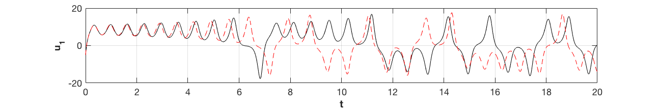
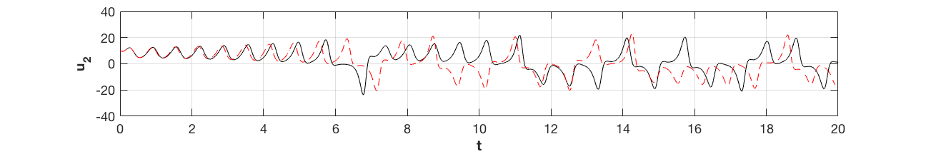
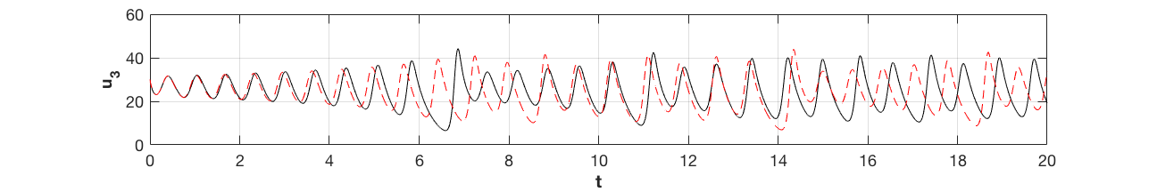
(a) $\sigma^{2}=0.1$

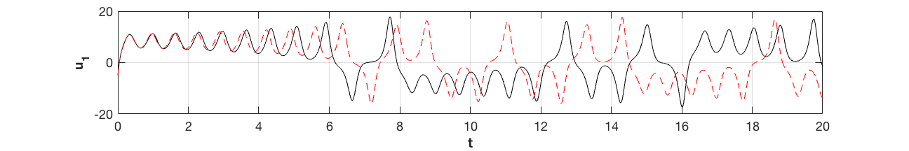
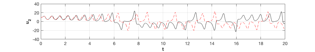
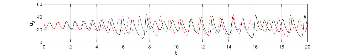
(b) $\sigma^{2}=0.5$

Figure 3.1: Lorenz system: Component-wise evolution of the trajectories. Solid line: the trajectory of the identified systems defined by: (a) Equation (3.4) and (b) Equation (3.5), respectively. Red dashed line: the “true” Lorenz attractor.

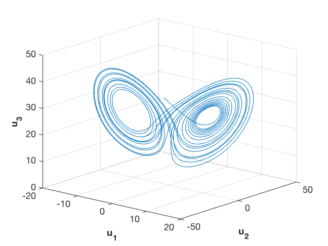
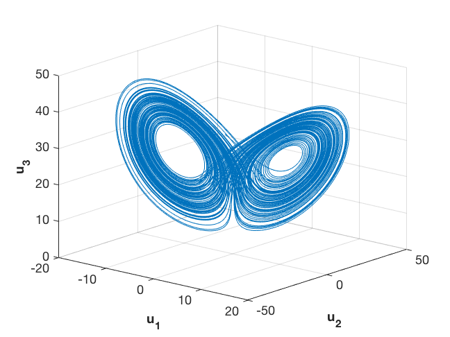
(a) The Lorenz attractor

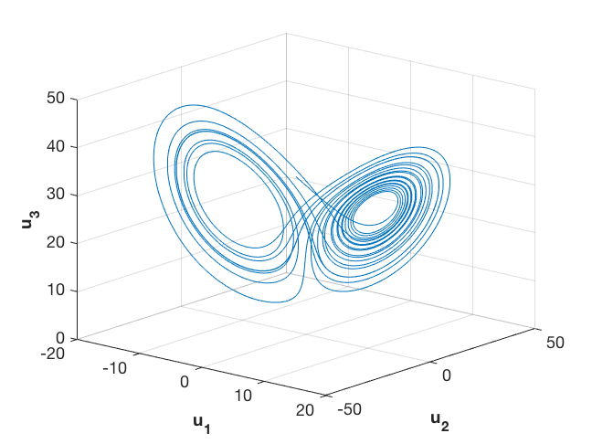
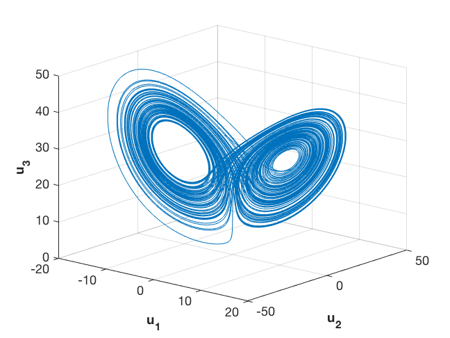
(b) The trajectory defined by Equation (3.4)

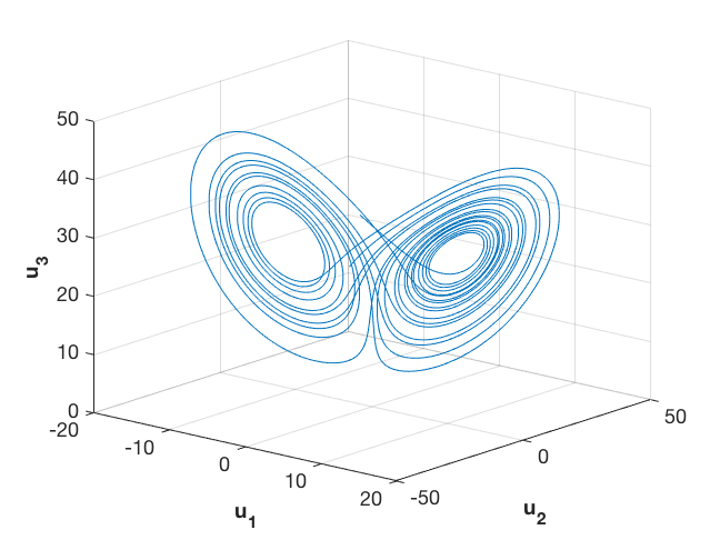
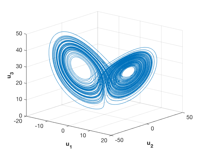
(c) The trajectory defined by Equation (3.5)

Figure 3.2: Lorenz System: Trajectories of the Lorenz system from $t=0$ to $t=20$ (left column) and from $t=0$ to $t=100$ (right column). (a) The “true” Lorenz attractor defined by Equation (3.1). (b) The trajectory defined by Equation (3.4), which is identified from data with additive noise $\sigma^{2}=0.1$. (c) The trajectory defined by Equation (3.5), which is identified from data with additive noise $\sigma^{2}=0.5$.

3.2 The Thomas System

Consider the Thomas system:

$$\begin{cases}\dot{u}_{1}=-0.18u_{1}+\sin(u_{2}),\\ \dot{u}_{2}=-0.18u_{2}+\sin(u_{3}),\\ \dot{u}_{3}=-0.18u_{4}+\sin(u_{1}).\end{cases}$$ (3.6)

which is a non-polynomial system whose trajectories form a chaotic attractor. We simulate $u(t)$ using the initial condition $u(0)=\begin{pmatrix}1,1,0\end{pmatrix}^{T}$ and by evolving the system using the Runge-Kutta method of order 4 up to time-stamp $t=100$ with time step $h=0.025$. We then add Gaussian noise to $u$ and obtain the observed noisy data $\tilde{u}(t)$:

$$\tilde{u}=u+\eta,\quad\eta\sim\mathcal{N}(0,\sigma^{2}).$$

Let $b$ be the numerical approximation of $\dot{u}$ which is defined by Equation (3.3). To identify the governing equation for the data generated by the Thomas system (e.g. the right-hand side of Equation (3.6)), we apply the algorithm to the linear system whose dictionary matrix $A=A(\tilde{u}(t))$ consists of three sub-matrices:

$$A=\begin{pmatrix}|&|&|\\ A_{P}&A_{\sin}&A_{\cos}\\ |&|&|\end{pmatrix},$$

where

$$A_{P} =\begin{pmatrix}|&|&|&|&&|\\ 1&P(\tilde{u}(t))&P^{2}(\tilde{u}(t))&P^{3}(\tilde{u}(t))&\cdots&P^{p_{1}}(\tilde{u}(t))\\ |&|&|&|&&|\end{pmatrix},$$

$$A_{\sin} =\begin{pmatrix}|&|&|&&|\\ \sin\left(P(\tilde{u}(t))\right)&\sin\left(P^{2}(\tilde{u}(t))\right)&\sin\left(P^{3}(\tilde{u}(t))\right)&\cdots&\sin\left(P^{p_{2}}(\tilde{u}(t))\right)\\ |&|&|&&|\end{pmatrix},$$

$$A_{\cos} =\begin{pmatrix}|&|&|&&|\\ \cos\left(P(\tilde{u}(t))\right)&\cos\left(P^{2}(\tilde{u}(t))\right)&\cos\left(P^{3}(\tilde{u}(t))\right)&\cdots&\cos\left(P^{p_{3}}(\tilde{u}(t))\right)\\ |&|&|&&|\end{pmatrix}.$$

Here, $P^{p}$ is defined by Equation (3.2), which denotes the matrix consisting of polynomials in $\tilde{u}$ of order $p$. The matrices $\sin(P^{p})$ and $\cos(P^{p})$ are obtained by applying the sine and cosine functions to each element of $P^{p}$, respectively.

With $p_{1}=3$, $p_{2}=p_{3}=1$, and $\lambda=0.1$, we apply the algorithm to data with different noise levels. The resulting approximations for $x$ are listed in Table 3.2. The identified systems are:

1. $\sigma^{2}=0.1$ (where ${\rm SNR}(u,\eta)=25.8469$):

   $$\begin{cases}\dot{u}_{1}=-0.1805u_{1}+1.0014\sin(u_{2})\\ \dot{u}_{2}=-0.1799u_{2}+1.0038\sin(u_{3})\\ \dot{u}_{3}=-0.1803u_{3}+0.9992\sin(u_{1})\end{cases}$$ (3.7)

   with $E(x)=0.0023$;

2. $\sigma^{2}=0.5$ (where ${\rm SNR}(u,\eta)=11.8738$):

   $$\begin{cases}\dot{u}_{1}=-0.1835u_{1}+1.0304\sin(u_{2})\\ \dot{u}_{2}=-0.1848u_{2}+0.9956\sin(u_{3})\\ \dot{u}_{3}=-0.1725u_{3}+0.9658\sin(u_{1})\end{cases}$$ (3.8)

   with $E(x)=0.0267$.

Table 3.2: The Thomas system: The recovered coefficients for two noise levels.

$A$	$\sigma^{2}=0.1$			$\sigma^{2}=0.5$
	$\dot{u}_{1}$	$\dot{u}_{2}$	$\dot{u}_{3}$	$\dot{u}_{1}$	$\dot{u}_{2}$	$\dot{u}_{3}$
$1$	0	0	0	0	0	0
$u_{1}$	-0.1805	0	0	-0.1835	0	0
$u_{2}$	0	-0.1799	0	0	-0.1848	0
$u_{3}$	0	0	-0.1803	0	0	-0.1725
$u_{1}^{2}$	0	0	0	0	0	0
$u_{1}u_{2}$	0	0	0	0	0	0
$u_{1}u_{3}$	0	0	0	0	0	0
$u_{2}^{2}$	0	0	0	0	0	0
$\vdots$	$\vdots$	$\vdots$	$\vdots$	$\vdots$	$\vdots$	$\vdots$
$u_{3}^{3}$	0	0	0	0	0	0
$\sin(u_{1})$	0	0	0.9992	0	0	0.9658
$\sin(u_{2})$	1.0014	0	0	1.0304	0	0
$\sin(u_{3})$	0	1.0038	0	0	0.9956	0
$\cos(u_{1})$	0	0	0	0	0	0
$\cos(u_{2})$	0	0	0	0	0	0
$\cos(u_{3})$	0	0	0	0	0	0

Observe that the identified system defined by Equation (3.7) is exact up to two significant digits. We simulate this system up to time-stamps $t=200$ and $t=1000$ and compare it with the trajectories of the Thomas system. We show the short-time evolution of the trajectories in Figure 3.3 and the long-time dynamics in Figure 3.4. It can be observed that although the coefficients are not exact, the trajectory of the identified system traces out a similar region to the exact trajectory in state-space.

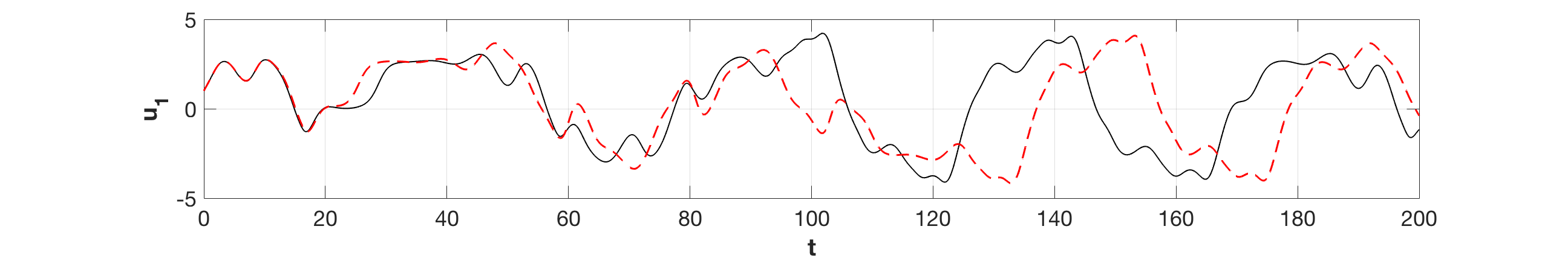
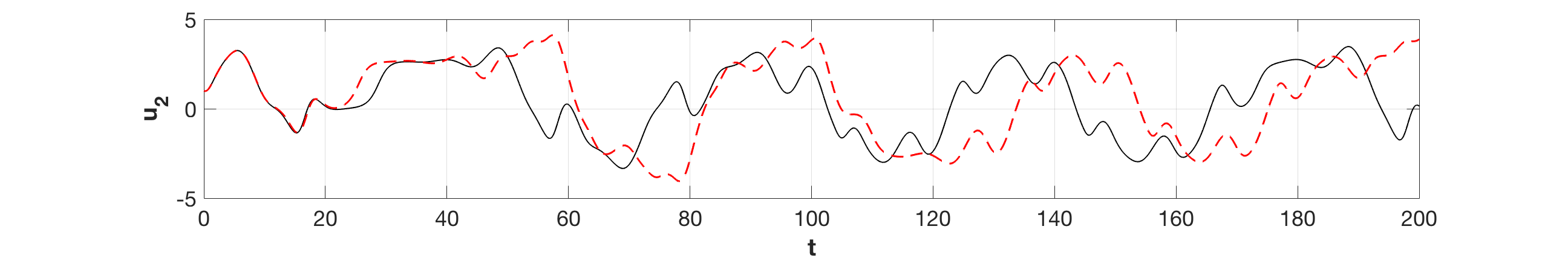
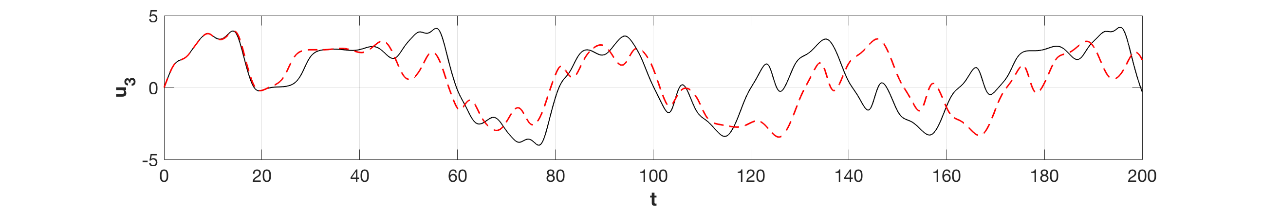
Figure 3.3: The Thomas system: Component-wise evolution of the trajectories. Solid line: the trajectory of the identified system defined by Equation (3.7). Red dashed line: the “true” Thomas trajectory.

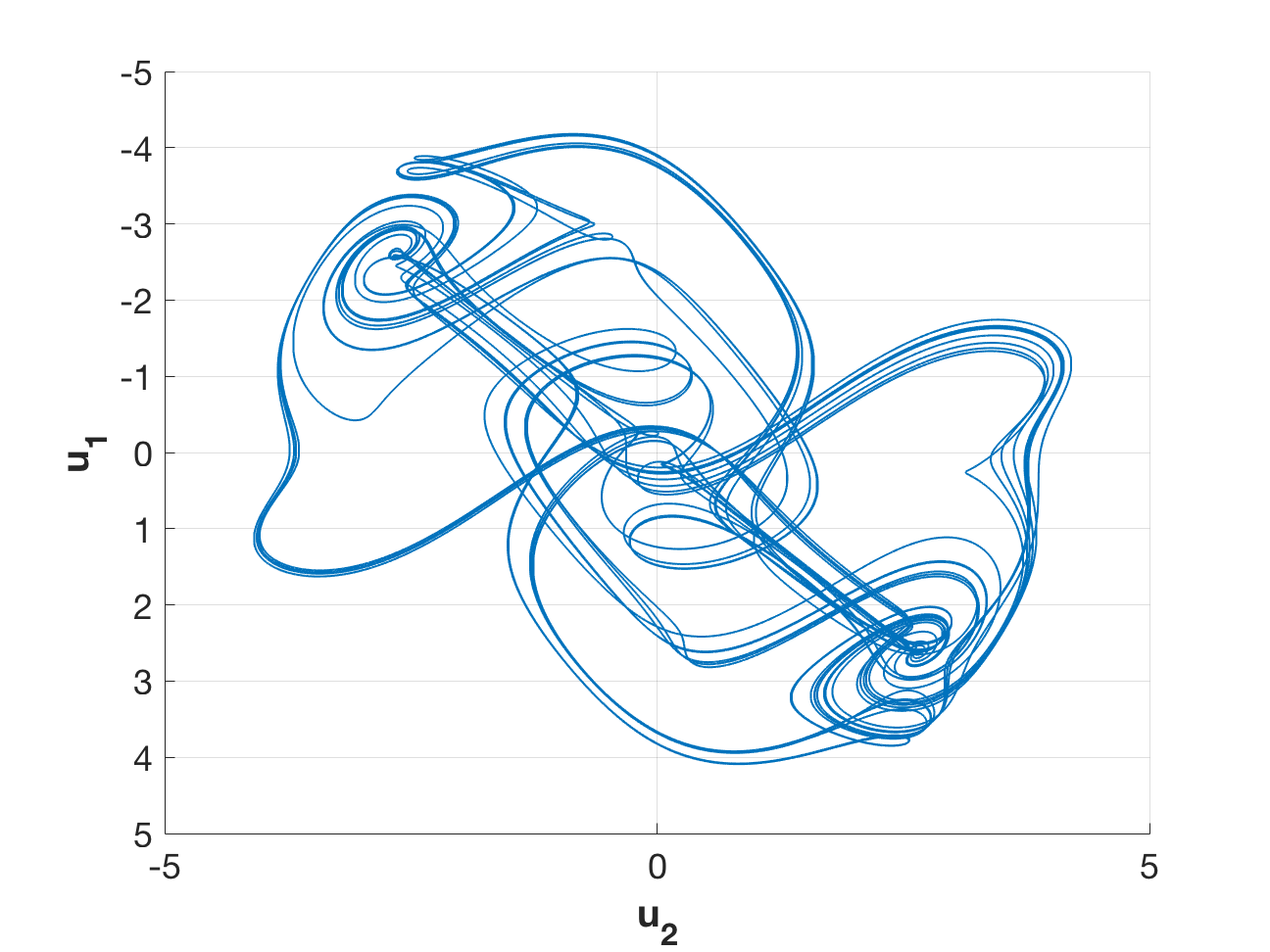
(a) The Thomas trajectory

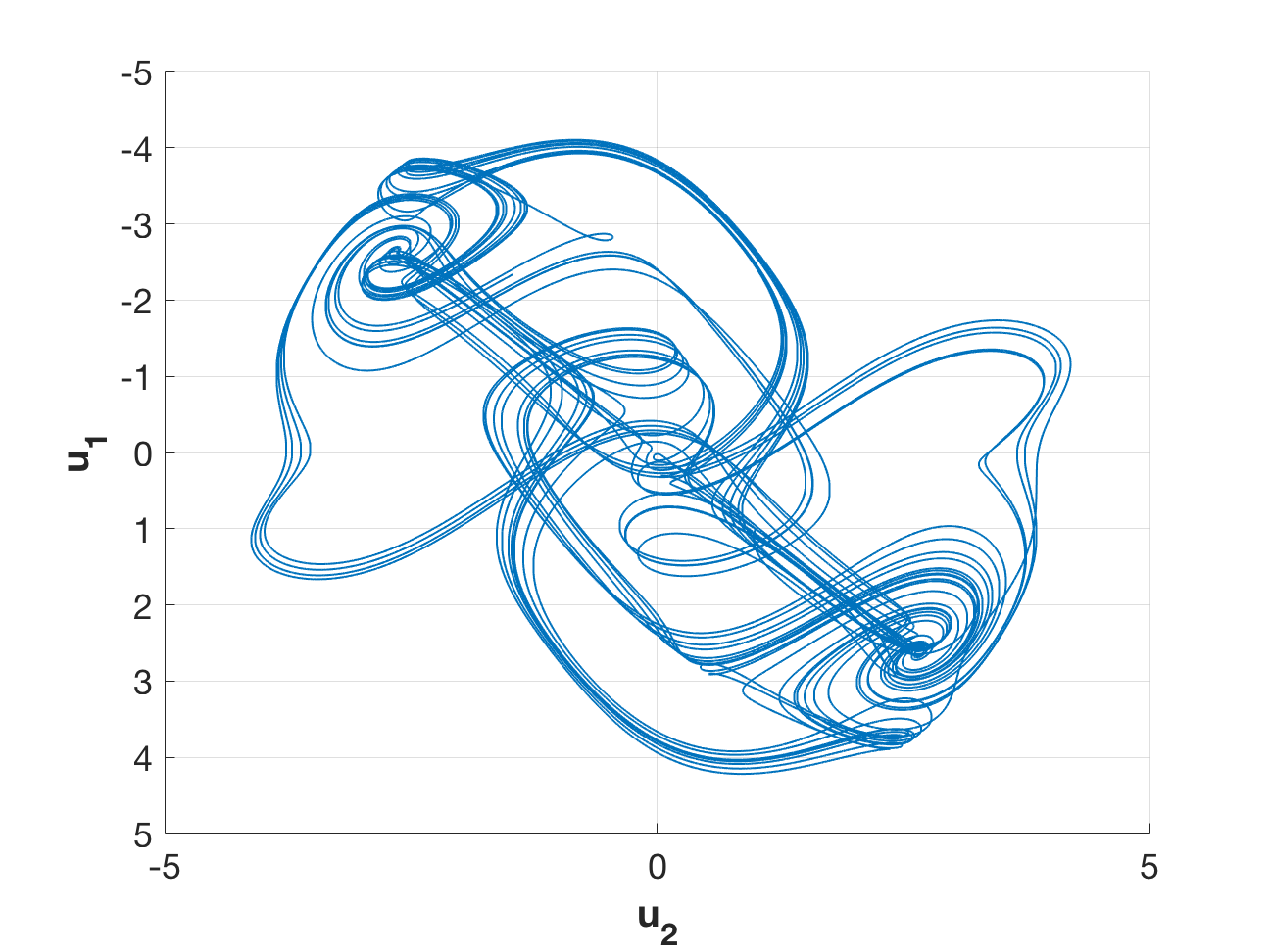
(b) The trajectory defined by Equation (3.7)

Figure 3.4: The Thomas system: Trajectories of the learned and “true” Thomas system from $t=0$ to $t=1000$ (right column). (a) The Thomas trajectory defined by Equation (3.6). (b) The trajectory defined by Equation (3.7), which is identified from data with additive noise $\sigma^{2}=0.1$.

4 Discussion

The SINDy algorithm proposed in [6] has been applied to various problems involving sparse model identification from complex dynamics. In this work, we provided several theoretical results that characterized the solutions produced by the algorithm and provided the rate of convergence of the algorithm. The results included showing that the algorithm approximates local minimizers of the $\ell^{0}$-penalized least-squares problem, and thus can be characterized through various sparse optimization results. In particular, the algorithm produces a minimizing sequence, which converges to a fixed-point rapidly, thereby providing theoretical support for the observed behavior. Several examples show that the convergence rates are sharp. In addition, we showed that iterating the steps is required, in particular, it is possible to obtain solutions through iterating that cannot be obtain via thresholding of the least-squares solution. In future work, we would like to better characterize the effects of noise, detailed in Section 3. It would be useful to have a quantifiable relationship between the thresholding parameter, the noise, and the expected recovery error.

References

- [1] Thomas Blumensath and Mike E. Davies. Iterative thresholding for sparse approximations. Journal of Fourier Analysis and Applications, 14:629–654, 2008.
- [2] Thomas Blumensath and Mike E. Davies. Iterative hard thresholding for compressed sensing. Applied and Computational Harmonic Analysis, 27:265–274, 2009.
- [3] Thomas Blumensath, Mehrdad Yaghoobi, and Mike E. Davies. Iterative hard thresholding and regularisation. 2007 IEEE International Conference on Acoustics, Speech and Signal Processing, 3:III–877, 2007.
- [4] Josh Bongard and Hod Lipson. Automated reverse engineering of nonlinear dynamical systems. Proceedings of the National Academy of Sciences, 104(24):9943–9948, 2007.
- [5] Lorenzo Boninsegna, Feliks Nüske, and Cecilia Clementi. Sparse learning of stochastic dynamic equations. ArXiv e-prints, December 2017.
- [6] Steven L. Brunton, Joshua L. Proctor, and J. Nathan Kutz. Discovering governing equations from data by sparse identification of nonlinear dynamical systems. Proceedings of the National Academy of Sciences, 113(15):3932–3937, 2016.
- [7] Steven L. Brunton, Joshua L. Proctor, and J. Nathan Kutz. Sparse identification of nonlinear dynamics with control (SINDYc). IFAC-PapersOnLine, 49(18):710–715, 2016.
- [8] Magnus Dam, Morten Brøns, Jens Juul Rasmussen, Volker Naulin, and Jan S. Hesthaven. Sparse identification of a predator-prey system from simulation data of a convection model. Physics of Plasmas, 24(2):022310, 2017.
- [9] Eurika Kaiser, J. Nathan Kutz, and Steven L. Brunton. Sparse identification of nonlinear dynamics for model predictive control in the low-data limit. ArXiv e-prints, November 2017.
- [10] Jean-Christophe Loiseau and Steven L. Brunton. Constrained sparse Galerki regression. Journal of Fluid Mechanics, 838:42–67, 2018.
- [11] Zichao Long, Yiping Lu, Xianzhong Ma, and Bin Dong. PDE-Net: Learning PDEs from data. ArXiv e-prints, October 2017.
- [12] Niall M. Mangan, Steven L. Brunton, Joshua L. Proctor, and J. Nathan Kutz. Inferring biological networks by sparse identification of nonlinear dynamics. IEEE Transactions on Molecular, Biological and Multi-Scale Communications, 2(1):52–63, 2016.
- [13] Niall M. Mangan, J. Nathan Kutz, Steven L. Brunton, and Joshua L. Proctor. Model selection for dynamical systems via sparse regression and information criteria. Proceedings of the Royal Society of London A, 473(2204):20170009, 2017.
- [14] Yannis Pantazis and Ioannis Tsamardinos. A unified approach for sparse dynamical system inference from temporal measurements. ArXiv e-prints, October 2017.
- [15] Markus Quade, Markus Abel, J. Nathan Kutz, and Steven L. Brunton. Sparse identification of nonlinear dynamics for rapid model recovery. ArXiv e-prints, March 2018.
- [16] Maziar Raissi and George Em Karniadakis. Hidden physics models: Machine learning of nonlinear partial differential equations. Journal of Computational Physics, 357:125–141, 2018.
- [17] Samuel H. Rudy, Steven L. Brunton, Joshua L. Proctor, and J. Nathan Kutz. Data-driven discovery of partial differential equations. Science Advances, 3:e1602614, 2017.
- [18] Hayden Schaeffer. Learning partial differential equations via data discovery and sparse optimization. Proceedings of the Royal Society of London A, 473(2197):20160446.
- [19] Hayden Schaeffer and Scott G. McCalla. Sparse model selection via integral terms. Physical Review E, 96(2):023302, 2017.
- [20] Hayden Schaeffer, Giang Tran, and Rachel Ward. Extracting sparse high-dimensional dynamics from limited data. ArXiv e-prints, July 2017.
- [21] Hayden Schaeffer, Giang Tran, and Rachel Ward. Learning dynamical systems and bifurcation via group sparsity. ArXiv e-prints, September 2017.
- [22] Hayden Schaeffer, Giang Tran, Rachel Ward, and Linan Zhang. Extracting structured dynamical systems using sparse optimization with very few samples. ArXiv e-prints, May 2018.
- [23] Michael Schmidt and Hod Lipson. Distilling free-form natural laws from experimental data. Science, 324(5923):81–85, 2009.
- [24] Mariia Sorokina, Stylianos Sygletos, and Sergei Turitsyn. Sparse identification for nonlinear optical communication systems: SINO method. Optics express, 24(26):30433–30443, 2016.
- [25] Robert Tibshirani. Regression shrinkage and selection via the lasso. Journal of the Royal Statistical Society. Series B (Methodological), pages 267–288, 1996.
- [26] Giang Tran and Rachel Ward. Exact recovery of chaotic systems from highly corrupted data. Multiscale Modeling & Simulation, pages 1108–1129.
- [27] Joel A. Tropp. Just relax: convex programming methods for identifying sparse signals in noise. IEEE Transactions on Information Theory, 52:1030–1051.