Reconstructing phenomenological distributions of compact binaries via gravitational wave observations

Abstract

Gravitational wave (GW) measurements will provide insight into the population of coalescing compact binaries throughout the universe. We describe and demonstrate a flexible parametric method to infer the event rate as a function of compact binary parameters, accounting for Poisson error and selection biases. Using synthetic data based on projections for LIGO and Virgo’s third observing run (O3), we discuss how well GW measurements could constrain the mass and spin distribution of coalescing neutron stars and black holes (BHs) in the near future, within the context of several phenomenological models described in this work. We demonstrate that only a few tens of events can enable astrophysically significant constraints on the spin magnitude and orientation distribution of BHs in merging binaries. We discuss how astrophysical priors or other measurements can inform the interpretation of future measurements. Using publicly available results, we estimate the event rate versus mass for binary black holes (BBHs). To connect to previously published work, we provide estimates including reported O2 BBH candidates, making several unwarranted but simplifying assumptions for the sensitivity of the network and completeness of the reported set of events. Consistent with prior work, we find BHs in binaries likely have low natal spin. With available results and a population favoring low spin, we cannot presently constrain the typical misalignments of the binary black hole population. All of the tools described in this work are publicly available and ready-to-use to interpret real or synthetic LIGO data, and to synthesize projected data from future observing runs.

I Introduction

The Advanced Laser Interferometer Gravitational Wave Observatory (LIGO)  Abbott et al. (2015) (The LIGO Scientific Collaboration) and Virgo Accadia and et al (2012); Acernese et al. (2015) detectors have and will continue to discover gravitational waves (GW) from coalescing binary black holes (BBHs) and neutron stars. Several tens of binary black holes and potentially neutron stars are expected to be seen in O3, LIGO’s next observing run, alone; and several hundreds more detections are expected over the next five years Abbott et al. (2016) (The LIGO Scientific Collaboration and the Virgo Collaboration); Abbott et al. (2016) (The LIGO Scientific Collaboration and the Virgo Collaboration). Already, the properties of the sources responsible – the inferred event rates, masses, and spins – have confronted other observations of black holes’ masses and spins Abbott et al. (2016) (The LIGO Scientific Collaboration and the Virgo Collaboration), challenged previous formation scenarios Abbott et al. (2016a) (The LIGO Scientific Collaboration and the Virgo Collaboration); Abbott et al. (2016) (The LIGO Scientific Collaboration and the Virgo Collaboration), and inspired new models Mandel and de Mink (2016); Marchant et al. (2016); Rodriguez et al. (2016a); Bird et al. (2016) and insights Kushnir et al. (2016); Lamberts et al. (2016) into the evolution of massive stars and the observationally accessible gravitational waves they emit Dvorkin et al. (2016); Abbott et al. (2016b) (The LIGO Scientific Collaboration and the Virgo Collaboration). Over the next several years, our understanding of the lives and deaths of massive stars over cosmic time will be transformed by the identification and interpretation of the population(s) responsible for coalescing binaries Abbott et al. (2016a) (The LIGO Scientific Collaboration and the Virgo Collaboration); Barack et al. (2018); Wysocki et al. (2018a), because measurements will enable robust tests to distinguish between formation scenarios Mandel and O’Shaughnessy (2010) with present Rodriguez et al. (2016b) and future instruments Breivik et al. (2016); Nishizawa et al. (2016).

During the first few years of discovery, substantial theoretical modeling challenges and the rapid pace of events suggest that GW observations could soon outpace theory. In this work, we introduce a flexible, concrete, and production-ready approach to infer compact binary merger rate and compact binary distribution, in the context of an (arbitrary) parametrized phenomenological model. We extend or employ previously proposed models Fishbach and Holz (2017); Talbot and Thrane (2018). We are motivated by how constraints on these phenomenological models enable us to address broad astrophysical questions—the mass and spin distribution of neutron stars and black holes, as imparted at their birth; the dominant formation mechanism for compact binaries, such as the role of dynamical versus isolated formation channels for binary black holes. To that end, we provide concrete demonstrations of how a few GW measurements will provide insights that enable sharp discrimination between proposed astrophysical alternatives, or measurements of their parameters. We use simple phenomenological arguments and calculations to characterize the information that these first few hundred observations should provide. Conversely, we provide simple approaches to extend our phenomenological approach in sophistication and complexity as several thousand compact binary mergers provide sharp constraints on their underlying properties. This approach complements inferences that work within a concrete model family as explored in other proof-of-concept investigations (see, e.g., Mandel and O’Shaughnessy (2010); O’Shaughnessy (2013); Stevenson et al. (2015); Belczynski et al. (2016a); Zevin et al. (2017); Barrett et al. (2018); Miyamoto et al. (2017); Wysocki et al. (2018a) and references therein).

GW measurements probe only a selection-biased part of the compact binary distribution. Previously reported estimates of the overall compact binary event rate rely on extrapolation away from the observed population, using some fixed model for the compact binary mass distribution Abbott et al. (2016) (The LIGO Scientific Collaboration and the Virgo Collaboration). In fact, the compact binary mass distribution and inferred event rate are strongly coupled. This paper provides the first self-consistent approach to infer both the compact binary event rate and parameter distribution; then it describes and explains the expected correlation in an accessible way.

Several recent studies have explored how well GW measurements can constrain the mass and spin distribution of binary black holes O’Shaughnessy (2013); Wysocki (2017); Mandel et al. (2017); Kovetz et al. (2017); Talbot and Thrane (2017); Farr et al. (2017); Fishbach and Holz (2017); Gerosa and Berti (2017); Fishbach et al. (2017); Stevenson et al. (2017); Abbott et al. (2016) (The LIGO Scientific Collaboration and the Virgo Collaboration); Vitale et al. (2017a); Farr et al. (2018). Our approach is novel insofar as it reconstructs both the strongly correlated event rate and the parameter distribution, making our method a robust tool to assess astrophysical formation scenarios. In our modeling, we focus on measuring the black hole (BH) spin magnitude and misalignment distribution, as a method to probe the formation scenarios for binary BHs. As first described in Mandel and O’Shaughnessy (2010), GW provide a unique opportunity to distinguish between isolated and dynamic formation mechanisms: measurements of the spin properties of the BHs Abbott et al. (2016a) (The LIGO Scientific Collaboration and the Virgo Collaboration); Rodriguez et al. (2016b); Vitale et al. (2017b); Stevenson et al. (2017); O’Shaughnessy et al. (2017); Talbot and Thrane (2017). The presence of a component of the BH spins in the plane of the orbit leads to precession of that plane. If suitably massive and significantly spinning, such binaries will strongly precess within the LIGO sensitive band. If BBHs are the end points of isolated binary star systems, they would be expected to contain BHs with spins preferentially aligned with the orbital angular momentum Kalogera (2000); O’Shaughnessy et al. (2017), and therefore rarely be strongly precessing. If, however, BBHs predominantly form as a result of gravitational interactions inside dense populations of stellar systems, the relative orientations of the BH spins with their orbits will be random, and some gravitational wave signals may be very strongly precessing. At this early stage, observations cannot firmly distinguish between these two scenarios, or more broadly other possible BBH formation mechanisms Abbott et al. (2016a) (The LIGO Scientific Collaboration and the Virgo Collaboration). These include the evolution of isolated pairs of stars Belczynski et al. (2016a, 2010); O’Shaughnessy et al. (2012); Dominik et al. (2012); Mandel and de Mink (2016); Marchant et al. (2016), dynamic binary formation in dense clusters Rodriguez et al. (2016a), and pairs of primordial black holes BHs Bird et al. (2016); see, e.g., Abbott et al. (2016a) (The LIGO Scientific Collaboration and the Virgo Collaboration) and references therein. Loosely speaking, however, the isolated evolution and globular cluster formation scenarios are the most well-developed and verifiable using independent observational constraints. More broadly, precise measurements of their properties will provide unique clues into how BHs and massive stars evolve Vitale et al. (2017b); Stevenson et al. (2017); Rodriguez et al. (2016b); Farr et al. (2017); Wysocki et al. (2018b); Breivik et al. (2016); Nishizawa et al. (2016).

This paper is organized as follows. In Sec. II we describe our techniques to infer compact binary populations, building upon inferences about parameters of individual events. Unlike prior work, we simultaneously reconstruct the event rate, mass distribution, and spin (vector) distribution. In Sec. III, we demonstrate our our population inference strategy with two examples. In the first, we perform a full end-to-end analysis of a synthetic GW data generated from a synthetic population of astrophysically distributed sources. In the second, using a tool to mimic how well we could constrain parameters of a candidate GW signal, we perform a large-scale investigation into how well GW measurements could constrain the mass and spin distribution of binary black holes. We find that the mass and spin distribution can be tightly constrained with only a few tens of events. By virtue of explicitly exploiting only some of the available information, our estimates are necessarily conservative. In Sec. IV, we apply our method to the currently reported binary black hole population. For simplicity, assuming the reported events to date represent a fair sample of the results of LIGO’s first two observing runs (O1 and O2), we corroborate previous results, finding black hole spins are likely small and that the black hole mass spectrum may have an upper bound. Due to small BH spins, except for GW151226, we can extract no information about typical BBH spin-orbit misalignments. We emphasize our demonstration uses a nonfinal sample for LIGO’s O2 survey: depending on that survey’s results, applying our methods to final O2 results could produce substantially different astrophysical conclusions. In Sec. V we briefly discuss the accuracy to which population parameters can be determined, and the surprisingly significant role of waveform systematics in the near future. After summarizing our conclusions in Sec. VI, we supply three appendixes. In Appendix A, we describe a robust, extensible procedure for generating synthetic posterior distributions for proposed GW events. This open-source procedure could be widely used to assess the viability of GW measurements to distinguish between proposed astrophysical channels. A subsequent short Appendix B describes how to generate synthetic populations of selection-biased GW sources using this procedure. Next, in Appendix C, following on and extending previous work, we use toy models for both the measurement process and source population to illustrate how well GW observations will constrain the mass and spin distribution of compact binaries, likely providing robust insights into compact object formation (e.g., BH natal spins and maximum masses) and binary formation mechanisms (e.g., dynamical over isolated).

II Method

II.1 Characterizing and inferring parameters of individual binary black holes

A coalescing compact binary in a quasicircular orbit can be completely characterized by its intrinsic parameters, namely its individual masses $m_{i}$ and spins $\bm{S}_{i}$, and its seven extrinsic parameters: right ascension, declination, luminosity distance, coalescence time, and three Euler angles characterizing its orientation (e.g., inclination, orbital phase, and polarization). In this work, we will also use the total mass $M=m_{1}+m_{2}$ and mass ratio $q$ defined in the following way:

$$q=m_{2}/m_{1},\quad\text{where }m_{1}\geq m_{2}.$$ (1)

We will also refer to two other commonly used mass parametrizations: the chirp mass $\mathcal{M}_{\text{c}}=(m_{1}m_{2})^{3/5}/(m_{1}+m_{2})^{1/5}$ and the symmetric mass ratio $\eta=m_{1}m_{2}/(m_{1}+m_{2})^{2}$. With regard to spin, we define an effective spin Damour (2001); Racine (2008); Ajith et al. (2011), which is a combination of the spin components along the orbital angular momentum direction $\hat{L}$, in the following way:

$$\chi_{\text{eff}}=(\bm{S}_{1}/m_{1}+\bm{S}_{2}/m_{2})\cdot\hat{\bm{L}}/M$$ (2)

where $\bm{S}_{1}$ and $\bm{S}_{2}$ are the spins on the individual BH. We will also characterize BH spins using the dimensionless spin variables

$$\bm{\chi}_{i}=\bm{S}_{i}/m_{i}^{2}.$$ (3)

We will express these dimensionless spins in terms of Cartesian components $\chi_{i,x},\chi_{i,y},\chi_{i,z}$, expressed relative to a frame with $\hat{z}=\hat{L}$ and (for simplicity) at the orbital frequency corresponding to the earliest time of astrophysical interest (e.g., an orbital frequency of $\simeq 10\,{\rm Hz}$).

When necessary, compact binary parameters are inferred through the use of Bayesian analysis via Rapid parameter Inference on gravitational wave sources via Iterative Fitting (RIFT) Lange et al. (2018), which reproduces the results of standard Monte Carlo techniques described in Abbott et al. (2016c) (The LIGO Scientific Collaboration and the Virgo Collaboration); Veitch et al. (2015) and references therein. For any event, fully characterized by parameters $x$, we can compute the (Gaussian) likelihood function $p(d|x)$ for detector network data $d$ containing a signal by using waveform models and an estimate of the (approximately Gaussian) detector noise on short timescales (see, e.g., Veitch et al. (2015); Abbott et al. (2016c) (The LIGO Scientific Collaboration and the Virgo Collaboration); Abbott et al. (2016d) (The LIGO Scientific Collaboration and the Virgo Collaboration) and references therein). In this expression $x$ is shorthand for the set of 15 parameters needed to fully specify a quasicircular BBH. The posterior probability distribution is therefore $p(x|d)\propto p(d|x)p(x)$, where $p(x)$ is the prior probability of finding a merger with different masses, spins, and orientations somewhere in the universe. These parameters $x$ can and are often described with alternate coordinate systems. We sometimes refer to the source luminosity distance $d_{L}$ or equivalently its source redshift $z$, and to the detector-frame or redshifted masses $m_{i,z}=m_{i}(1+z)$. (To distinguish from the detector-frame masses, we will sometimes refer to $m_{i}$ as the source-frame binary masses.) LIGO-Virgo analyses have adopted a fiducial prior $p_{\rm ref}(x)$ that is uniform in orientation, in luminosity distance cubed, in redshifted mass, in spin direction (on the sphere), and, importantly for us, in spin magnitude Veitch et al. (2015); Abbott et al. (2016c) (The LIGO Scientific Collaboration and the Virgo Collaboration). Using standard Bayesian tools Abbott et al. (2016c) (The LIGO Scientific Collaboration and the Virgo Collaboration); Veitch et al. (2015), one can produce a sequence of independent, identically distributed samples $x_{n,s}$ ($s=1,2,\ldots,S$) from the posterior distribution $p(x|d)$ for each event $n$; that is, each $x_{n,s}$ is drawn from a distribution proportional to $p(d_{n}|x_{n})p_{\rm ref}(x_{n})$. Typical calculations of this type provide $\lesssim 10^{4}$ samples Abbott et al. (2016c) (The LIGO Scientific Collaboration and the Virgo Collaboration); Veitch et al. (2015) from which the posterior probability distribution is inferred.

For other examples involving purely synthetic observing scenarios, we perform this procedure with a familiar Fisher matrix approximation for the form of $p(d|x)$ as a function of $x$ Cutler and Flanagan (1994); Poisson and Will (1995); Cho et al. (2013); see Appendix A for details.

II.2 Population inference

We use Bayesian inference to constrain the mass and spin distributions of the astrophysical population of BBHs. To do this, we assume that the distribution is one of a family of distributions, parametrized by $\Lambda$ and scaled by some overall rate $\mathcal{R}=\mathrm{d}N/(\mathrm{d}t\,\mathrm{d}V_{\mathrm{c}})$, which is constant in comoving volume $V_{\mathrm{c}}$. Each BBH in the population has properties denoted by $\lambda\equiv(m_{1},m_{2},\bm{\chi}_{1},\bm{\chi}_{2})$

Ultimately we are interested in determining the likelihood of the astrophysical BBH population having a given merger rate $\mathcal{R}$ and obeying a given parametrization $\Lambda$, given the data for $N$ detections, $\mathcal{D}=(d_{1},\ldots,d_{N})$. This likelihood, $\mathcal{L}(\mathcal{R},\Lambda)\equiv p(\mathcal{D}\mid\mathcal{R},\Lambda)$, is that of an inhomogeneous Poisson process

$$\mathcal{L}(\mathcal{R},\Lambda)\propto e^{-\mu(\mathcal{R},\Lambda)}\prod_{n=1}^{N}\int\mathrm{d}\lambda\,\ell_{n}(\lambda)\,\mathcal{R}\,p(\lambda\mid\Lambda),$$ (4)

where $\mu(\mathcal{R},\Lambda)$ is the expected number of detections under a given population parametrization $\Lambda$ with overall rate $\mathcal{R}$ and where $\ell_{n}(\lambda)=p(d_{n}|\lambda)$ is the likelihood of data $d_{n}$ given binary parameters $\lambda$. A derivation for $\mu$ is given in Sec. II.3.

Using Bayes’ theorem, $p(\mathcal{R},\Lambda\mid\mathcal{D})\propto p(\mathcal{R},\Lambda)\,\mathcal{L}(\mathcal{R},\Lambda)$, one may obtain a posterior distribution on $\mathcal{R}$ and $\Lambda$, after assuming some prior $p(\mathcal{R},\Lambda)$. To avoid computing the normalization constant, we instead draw samples from the posterior distribution via Goodman and Weare’s affine invariant Markov chain Monte Carlo (MCMC) ensemble sampler Goodman and Weare (2010), as implemented in the Python package emcee Foreman-Mackey et al. (2013).

II.3 Estimate for $VT$

Current LIGO-Virgo search sensitivity is well approximated by a familiar approximation: a source will typically be detected if the estimated signal to noise (SNR) of the second-most-sensitive detector is greater than $8$; see, e.g., Abadie et al (2010) (The LIGO Scientific Collaboration and the Virgo collaboration) and references therein. Using this approximation, one can directly evaluate the characteristic volume within which a source will be detected Finn and Chernoff (1993); for nonspinning BH binaries, this estimate is in reasonable agreement with detailed calculations of search sensitivity Abbott et al. (2016) (The LIGO Scientific Collaboration and the Virgo Collaboration). In this work, we therefore adopt the same approximation. Specifically, we estimate the orientation-averaged sensitive 3-volume $V$ to which a search is sensitive by the integral Abbott et al. (2016a) (The LIGO Scientific Collaboration and the Virgo Collaboration); O’Shaughnessy et al. (2010a)

$$V(\lambda)=\int P(<D(z)/D_{h}(\lambda))\frac{\mathrm{d}V_{\mathrm{c}}}{\mathrm{d}z}\frac{\mathrm{d}z}{1+z},$$ (5)

where $D(z)$ is the luminosity distance for redshift $z$; $D_{h}(m_{1}(1+z),m_{2}(1+z))$ is the horizon distance to which the source can be seen; $V_{\mathrm{c}}$ is the comoving volume; $z$ is the redshift of the merger event; and the cumulative distribution $P(>w)=\int_{w>w(\Omega,\iota,\psi)}d\Omega d\psi d\cos\iota$ is a cumulative distribution for $w=8/\rho$ where $\rho$ is the signal to noise ratioFinn and Chernoff (1993); O’Shaughnessy et al. (2010a); Dominik et al. (2015). Using this definition for $V$, we expect that for a uniform comoving merger rate $\mathcal{R}$ (e.g., in units of $\mathrm{Gpc}^{-3}\,\mathrm{yr}^{-1}$), and after observing at this sensitivity for a time $T$ the average number of detections will be

$$\mu(\mathcal{R},\Lambda)=\int(VT)(\lambda)\mathcal{R}p(\lambda\mid\Lambda)\mathrm{d}\lambda,$$ (6)

where $p(\lambda\mid\Lambda)$ is the probability density function for a random binary in the Universe to have intrinsic parameters $\lambda$. In this expression, $\Lambda$ denotes the parameters that characterize the distribution from which all coalescing binaries are drawn. To calculate the horizon distance $D_{h}$ and hence $V$ for each combination of candidate binary parameters, we use the IMRPhenomD gravitational waveform approximation Husa et al. (2016); Khan et al. (2016).

The procedure described above allows us to estimate $V$ for any nonprecessing binary. Fig. 1 shows this estimate as a function of the component masses, based on a single LIGO detector operating at O1 sensitivity. Motivated by LIGO observations to date, however, we assume black holes will not be rapidly spinning. In these circumstances, spin has at best a modest impact on the sensitive volume; further complications due to precession would be expected to be smaller still Brown et al. (2012); O’Shaughnessy et al. (2010b).

Though we pursue a semianalytic estimate for $VT$ and hence the expected number of GW-detected events, detailed analysis of gravitational wave searches in real data with synthetic sources can evaluate $\mu$ and hence the search sensitivity directly Biswas et al. (2009); Abbott et al. (2016) (The LIGO Scientific Collaboration and the Virgo Collaboration); Abbott et al. (2016) (The LIGO Scientific Collaboration and the Virgo Collaboration); Tiwari (2018). Such an approach will be particularly necessary when search selection biases (e.g., due to detector noise non-Gaussianity) cause the search sensitivity threshold to deviate away from the simple SNR threshold described here.

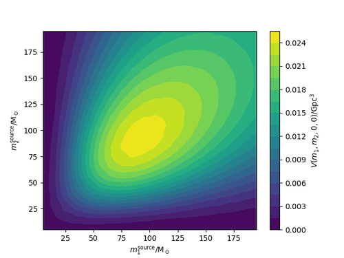
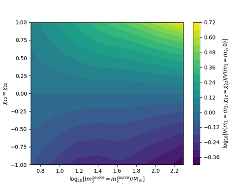
Figure 1: Estimated sensitive comoving volume ($V$) versus mass and spin. Left: Sensitive comoving volume $V$ at O1 sensitivity for nonspinning BBHs, in cubic giga-parsecs. Right: Sensitive comoving volume for equal-mass, equal-spin, nonprecessing BBHs, relative to the zero-spin case. Note that $V$ is strictly increased (decreased) if $\chi_{i,z}>0$ ($<0$), with higher mass making the effect more pronounced.

II.4 Examples of phenomenological population models

Motivated by the qualitative features of predictions produced by detailed binary formation calculations, several groups have proposed purely or weakly phenomenological models for the binary mass distribution Fishbach and Holz (2017); Abbott et al. (2016) (The LIGO Scientific Collaboration and the Virgo Collaboration); Fishbach and Holz (2017); Talbot and Thrane (2018); Christian et al. (2018). Following Abbott et al. (2016) (The LIGO Scientific Collaboration and the Virgo Collaboration); Fishbach and Holz (2017), we adopt a pure truncated power law for the relative intrinsic probability $p(m_{1},m_{2})$ for the source-frame masses in $m_{1}$ and $m_{2}$. Departing from previous work, we assume the probability density is nonzero only in a region $m_{\mathrm{min}}\leq m_{2}\leq m_{1}\leq m_{\mathrm{max}}$, and $m_{1}+m_{2}\leq M_{\mathrm{max}}$. Unless otherwise noted, we assume that $M_{\mathrm{max}}$ is a property of the detector, not astrophysics, and following the conservative scenario described in Fishbach and Holz (2017) fix it at $200\mathrm{M}_{\odot}$. With these assumptions, our mass distribution model has parameters $\alpha_{m},k_{m},m_{\rm min},m_{\rm max}$ and a functional form

$$p(m_{1},m_{2}) =\frac{(m_{2}/m_{1})^{k_{m}}m_{1}^{-\alpha_{m}}}{(m_{1}-m_{\mathrm{min}})}$$

$$\times C(\alpha_{m},k_{m},m_{\mathrm{min}},m_{\mathrm{max}},M_{\mathrm{max}})$$ (7)

inside our mass limits and zero elsewhere, representing a truncated power law in $m_{1}$ with index $-\alpha_{m}$ and a simple power-law conditional distribution $p(m_{2}|m_{1})$ in secondary mass. The normalization constant $C$ is defined so $\int_{A}dm_{1}dm_{2}p(m_{1},m_{2})dm_{1}dm_{2}=1$. Unless otherwise noted, we will adopt $k_{m}=0$ in this work. Because GW networks are much more sensitive to more massive BHs with $M\gtrsim 200\mathrm{M}_{\odot}$, this model and its fiducial choices (e.g., $\alpha_{m}\simeq 2$) produce a detected merger distribution $\propto Rp(m_{1},m_{2})VT$ which is roughly uniform over a wide range of masses, usually terminated by the specific cutoff choices $m_{\mathrm{max}},m_{\mathrm{min}}$ rather than by selection biases against low mass black holes or the rarity of massive BBHs. In the analysis described below, we leave $M_{\mathrm{max}}$ fixed.

Motivated by binary neutron star observations as well as the desire to reproduce arbitrary substructure and features in the mass distribution, we will also examine Gaussian mass distributions in component mass $m_{i}$

$$p_{G}(m_{1})=\mathcal{N}(\overline{m},\sigma_{m})(m_{1})$$ (8)

which is characterized by its mean value $\overline{m}$ and variance $\sigma_{m}$. In this work, we will typically explore the special case of $p(m_{1},m_{2})=p_{G}(m_{1})p_{G}(m_{2})$ and apply this distribution to the case of binary neutron stars, where the narrow width $\sigma$ relative to the mean $\overline{m}$ implies the distribution has effectively no support for undesirable regions (e.g., $m<0$). Finally, for complete generality, we also discuss mixtures of mass distributions, including Gaussian mixture models as previously employed in Wysocki (2017):

$$p(m_{1},m_{2}|\Lambda)=\sum_{\alpha}w_{\alpha}p_{\alpha}(m_{1},m_{2}|\Lambda_{\alpha})$$ (9)

This latter approach allows complete generality and, with suitable smoothing priors on $w$, the ability to reproduce arbitrarily complicated mass distributions and circumvent systematic limitations due to our choice of model. In particular, these more generic models would allow us to reproduce features previously proposed in the literature, including overabundances at specific masses near the pair-instability supernova threshold Fraley (1968); Fryer et al. (2001); Woosley et al. (2002, 2007); Kasen et al. (2011); Belczynski et al. (2016b).

For binary black hole spins, we adopt a simple flexible phenomenological model for each BH spin magnitude $\chi_{i}$: a beta distribution,

$$p(\chi_{i}\mid\alpha_{\chi_{i}},\beta_{\chi_{i}})=\frac{\chi_{i}^{\alpha_{\chi_{i}}-1}\,(\chi_{\rm max}-\chi_{i})^{\beta_{\chi_{i}}-1}}{\mathrm{B}(\alpha_{\chi_{i}},\beta_{\chi_{i}})\chi_{\rm max}^{\beta+\alpha+1}}$$ (10)

with unknown shape parameters $\alpha_{\chi_{i}}$ and $\beta_{\chi_{i}}$ ($i=1,2$). This tractable two-parameter distribution allows us to fit to the observed mean and variance—all that the sparse sample of existing observations will allow. In this work, we for simplicity assume both black hole spins are drawn from the same distribution and $\chi_{\rm max}=1$. Likewise, for simplicity we adopt the unphysical but easily described parametrization of the spin-orbit misalignment $\theta_{i}=\arccos\hat{\mathbf{L}}\cdot\hat{\mathbf{S}}_{i}$ proposed by Talbot and Thrane Talbot and Thrane (2017): a unimodal distribution based on a Gaussian in $\cos\theta$ that smoothly deforms into a uniform distribution in the limit of large $\sigma_{\chi_{i}}$:

$$p(\cos\theta_{i}\mid\sigma_{\chi_{i}})\propto\mathcal{N}(\cos\theta_{i};1,\sigma_{\chi_{i}}),$$ (11)

When using this model, we assume the polar angles $\phi_{i}$ of each spin vector relative to the orbital angular momentum direction $\hat{L}$ are uniformly distributed between $0,2\pi$. In this work, we assume BH spins are drawn from the same spin misalignment distribution $\sigma_{\chi_{1}}=\sigma_{\chi_{2}}$. In this approach, as in our parameter inference, all spins are assumed specified at a gravitational wave frequency $f_{\rm ref}=20\,{\rm Hz}$. No compelling reason exists that astrophysical formation processes should cause binaries of different masses and spins to be drawn from a single, universal misalignment distribution at an arbitrary reference frequency $f_{\rm ref}$; see, e.g., Wysocki et al. (2018a); Rodriguez et al. (2018) for more detailed models. That said, this phenomenological approach is qualitatively consistent with the kinds of misalignments produced by binary SN natal kicks (e.g., $1-\cos\theta_{i}\lesssim 0.1$ for BH natal kicks of order $50\,{\rm km/s}$ O’Shaughnessy et al. (2017)), allowing us a simple way to characterize whether observations support or disfavor plausible amounts of spin-orbit misalignment.

II.5 Useful phenomenological parameters

Observations will constrain combinations of these phenomenological parameters which reflect clear physical features in the observed (selection-biased) distribution of binary black holes. We can better characterize what we learn from GW observations early on by adopting coordinates conforming to these features.

For example, we could have mixture model [Eq. (9)] consisting only of elements with distinctive features, each characterizing a distinctive subpopulation of BHs. Such subpopulations might be BHs near the pair-instability supernova peak, binary neutron stars, and a population of binaries with a continuous mass spectrum formed through hierarchical growth in globular clusters (see, e.g., Miller and Hamilton (2002); Gerosa and Berti (2017); Fishbach and Holz (2017) and references therein). In such a scenario, observations quickly constrain each element, leveraging their distinctive features to identify the relative rates ${\cal R}w_{\alpha}$ and the subpopulations from each domain to constrain that region’s parameters. For the first few tens of events, these observations will principally constrain the mean and variance of the detection-weighted subpopulation $p_{\alpha}(m_{1},m_{2})VT$. We therefore expect that the following coordinate system will produce roughly uncorrelated observables, for a typical model: (a) the relative rates ${\cal R}w$ for different subpopulations; (b) the mean chirp mass $\overline{\mathcal{M}_{\text{c}}}_{\alpha}$, symmetric mass ratio $\overline{\eta}_{\alpha}$, effective spin $\overline{\chi}_{\rm eff,\alpha}$, and mean spin $\overline{\chi}$ in each subpopulation, based on our understanding of GW measurement errors; and (c) the respective widths $\Sigma_{\mathcal{M}_{\text{c}},\alpha}$, $\Sigma_{\eta,\alpha}$, $\Sigma_{\chi_{\mathrm{eff}},\alpha}$, $\Sigma_{\chi}$, where we adopt uppercase to distinguish between these symbols and our model hyperparameters. In Appendix C, we use order-of-magnitude arguments to explain how reliably each of these quantities can be measured.

In the context of our fiducial single-component model, we adopt a reference mass $m_{1}=m_{\rm ref}=15M_{\odot}$ and characterize the overall event rate not by its normalization, which depends on unobserved binaries with high and low masses, but by the event rate ${\cal R}p(m_{\rm ref})$ of binaries whose primary $m_{1}$ has a mass comparable to GW151226 Abbott et al. (2016a). We identify other natural coordinates for the distribution of $m_{1}$ via its detection-weighted cumulative distribution ${\cal P}(<m_{1})$:

$${\cal P}(<x)=\frac{\int d\lambda V(\lambda)p(\lambda)\Theta(x-m_{1}(\lambda))}{\int d\lambda V(\lambda)p(\lambda)}$$ (12)

The mass corresponding to the upper (lower) bound of the 90% symmetric detection-weighted probability on $m_{1}$ serves as a proxy for $m_{\mathrm{max}}$ ($m_{\mathrm{min}}$) which is directly observable and thus a more natural coordinate. In this work, we emphasize the upper bound $m_{*}$ of the detection-weighted mass distribution:

$${\cal P}(m_{*})\equiv 0.95$$ (13)

For BH spins, closed-form expressions for the appropriate mean values and variances are generally not available for arbitrary selection biases $VT$; however, to the extent that $VT$ depends only weakly on BH spin, our model for BH spins and misalignments [Eqs. (10,11)] implies that

$$\overline{\chi} \simeq\frac{\alpha_{\chi}}{\alpha_{\chi}+\beta_{\chi}}$$ (14a)

$$\Sigma_{\chi}^{2} \simeq\frac{\alpha_{\chi}\beta_{\chi}}{(\alpha_{\chi}+\beta_{\chi})^{2}(\alpha_{\chi}+\beta_{\chi}+1)}$$ (14b)

$$\overline{\chi}_{\rm eff} \simeq\overline{\chi}\overline{\cos\theta}$$ (14c)

$$\overline{\cos\theta} \simeq\frac{{\rm erf}(\sqrt{2}/\sigma)+2\sigma(e^{-2/\sigma^{2}}-1)/\sqrt{2\pi}}{{\rm erf}(\sqrt{2}/\sigma)}$$ (14d)

for our fiducial case where both BH spins are drawn from the same distributions; in these expressions, $\Sigma_{\chi}^{2}$ refers to the variance of the one-dimensional $\chi$ distribution, while $\bar{\chi}$ refers to its mean.

II.6 Interpreting results: Posterior predictive distributions and revised priors

If we ask any question about compact binary properties $x$ rather than model hyperparameters $\Lambda$, the only quantity that appears in our posterior inferences $p(\Lambda|\{d\})$ informed by our observations $\{d\}$ is the posterior predictive distribution $p_{\rm ppd}(x|\{d\})$:

$$p_{ppd}(x|\{d\})=\int d\Lambda p(x|\Lambda)p(\Lambda|\{d_{k}\})$$ (15)

The posterior predictive distribution (PPD) encodes our best estimates of the properties of any randomly selected future binary, based on observations to date and accounting for our initial prior knowledge about $\Lambda$. Unlike the model parameters themselves, which may be highly degenerate and lack physical meaning, the PPD provides an unambiguous estimate for how likely different binary parameters are, given our knowledge. Note that by design, the PPD is a probability distribution and, folding in all uncertainties, does not have an error estimate.

As events accumulate, we can use posterior constraints $p(\Lambda|\{d\}_{k})$ on model hyperparameters $\Lambda$ based on the first $k=1\cdots N$ observations to provide a nuanced, observationally revised perspective on future measurements $k>N$. These prior insights can be particularly powerful when individual future measurements are only weakly informative about certain binary parameters such as the mass ratio or spin; see, e.g., Vitale et al. (2017c); Williamson et al. (2017) for examples.

To be concrete, our usual population inferences are performed using a single fiducial choice of reference prior $p_{\rm ref}(x)=p(x|\Lambda_{\rm ref})$: the posterior is $p(x|d_{k},\Lambda_{*})=p(d_{k}|x)p(x|\Lambda_{*})/\int p(d|x)p(x|\Lambda_{\rm ref})$. We exploit prior measurements via

$$p(x|d_{k},\{d\})=\frac{p(d_{k}|x)\int d\Lambda p(x|\Lambda)p(\Lambda|\{d_{k}\})}{\int dxp(d_{k}|x)\int d\Lambda p(x|\Lambda)p(\Lambda|\{d_{k}\})}$$ (16)

In this expression, the numerator $\int d\Lambda p(x|\Lambda)p(\Lambda|\{d_{k}\})$ is the posterior predictive distribution described above.

III Controlled tests with synthetic populations and measurements

To demonstrate our method can infer population parameters, we perform several validation studies using toy models which mimic key features of real gravitational wave observations. These completely controlled illustrations also let us highlight what can be inferred and why about the mass and spin distribution, within the context of our approach. Finally, these examples allow us to demonstrate how population inference can strongly inform the interpretation of individual future GW observations.

III.1 BNS mass and (aligned) spin distribution

For each component of a binary neutron star (BNS), observations of galactic pulsars suggest that the component masses are drawn from a Gaussian distribution with mean $1.33M_{\odot}$ and standard deviation $0.09M_{\odot}$ Özel and Freire (2016). Observations of pulsars and theoretical models of pulsar spin-down suggest that if both NS are not recycled, then their dimensionless spins will be small [$\simeq\mathcal{O}(0.05)$]. Under the assumption that NS spins are parallel to their orbital angular momentum, we construct a synthetic population drawn from this phenomenological model; construct synthetic observations for each binary, recovering 13 synthetic sources based on a three-detector advanced LIGO/Virgo network using a threshold set by the second-most-sensitive detector’s recovered amplitude; perform full GW inference on each source using RIFT Lange et al. (2018); and, with the resulting posterior distributions, use the techniques of Sec. II to infer the underlying NS mass and spin distribution. In our reconstruction, we assume both components of a NS binary are independently drawn from a Gaussian distribution with unknown mean and variance; and with spins $\chi_{i,z}$ drawn from a beta distribution with unknown mean and variance, such that $|\chi_{i,z}|\leq 0.05$.

Fig. 2 shows the synthetic measurements used as inputs in our calculation. These synthetic measurements incorporate significant uncertainty in each source’s redshift, which contributes to the overall uncertainty in each binary’s chirp mass. For each neutron star in our synthetic population, we use the APR4 equation of state to calculate each neutron star’s tidal deformability $\lambda_{i}=\lambda(m|\text{APR4})$. We generate and recover our synthetic sources with IMRPhenomD_NRTidal Dietrich et al. (2019). Fig. 3 compares our recovered NS mass and spin distribution. When inferring source parameters, our waveform model and parameter inferences include the effects of NS tides, treating each NS tidal deformability $\lambda_{i}$ as a free parameter. Despite considerable uncertainties in each measurement, each BNS observation constrains that binary’s chirp mass reasonably well, to an accuracy $\sigma_{\mathcal{M}_{\text{c}}}\simeq 0.05M_{\odot}$, dominated by uncertainty in source redshift. Because GW measurements are only weakly informative about the mass ratio, these measurements each constrain the total mass to be $m_{1}+m_{2}\simeq 2^{6/5}\mathcal{M}_{\text{c}}$ to an accuracy $\sigma_{\mathcal{M}_{\text{c}}}2^{6/5}$; averaging all such observations, we can deduce the mean NS mass $\bar{m}$. With $n=13$ such measurements, we expect to constrain the mean mass of the population to a 1 standard deviation accuracy $\sqrt{\sigma_{\mathcal{M}_{\text{c}}}^{2}2^{12/5}/4+\sigma^{2}}/\sqrt{n}\simeq 0.027M_{\odot}$, which compares favorably to $0.02M_{\odot}$, the standard deviation of our Bayesian estimate for $\bar{m}$ . (A similar analysis shows that we constrain the NS population standard deviation $\sigma_{m}$ almost entirely through these one-dimensional chirp mass constraints.) Because GW measurements have a smaller statistical uncertainty than the astrophysical population width in total mass, the accuracy to which we constrain the mean NS mass is dominated by a simple frequentist error estimate ($\sigma/\sqrt{n}$), allowing us to reliably project the information we will extract about NS masses from future GW observations.

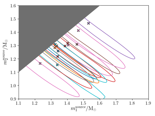
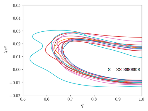
Figure 2: Source information for our synthetic BNS population: For each synthetic signal used in the BNS population reconstruction calculation described in Sec. III.1, these two panels show the true injected source-frame parameters (as crosses) and posterior distributions (contours of their 95% highest posterior density regions). Each color corresponds to a different source. Source parameters have been inferred using full Bayesian parameter inference via RIFT, as described in the text.

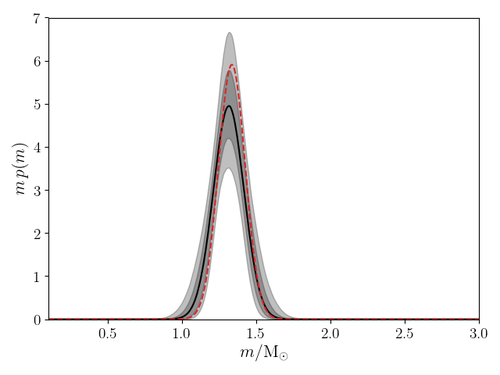
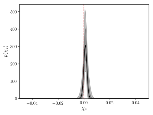
Figure 3: Recovered properties of NS mass and spin distribution: For the synthetic population of BNS sources illustrated in Fig. 2, this figure shows the recovered mass distribution (top figure) and spin distribution parameters (bottom figure) derived using the Gaussian mass and $\beta$-distribution spin model described in the text. The solid line indicates the median distribution; the shaded regions indicate the 68% and 95% credible intervals. Red dashed lines denote the true underlying distribution. In the case of spin, note that the truth is a delta function at zero, so it would require an infinite number of detections to fall within the constraints on this plot.

The measurement accuracy for GW measurements of BNS has been long known Poisson and Will (1995), and their implications for astrophysics (e.g., mass and BNS spin distributions) have been immediately apparent; see, e.g., O’Shaughnessy et al. (2014); Hannam et al. (2013); Zhu et al. (2018) and references therein. We provide the first end-to-end demonstration of how well binary NS population parameters can be measured, using a detailed waveform model at a level where waveform systematics should not dramatically impact the mass, spin, or tidal parameter inferences being performed. By contrast, many previous studies focusing on NS tidal deformation have demonstrated that waveform systematics could bias inferences Wade et al. (2014); Favata (2014); Lackey and Wade (2015), if not controlled. Only recently have systematic errors between waveform models diminished enough to enable consistent infererence; see, e.g., The LIGO Scientific Collaboration et al. (2019).

Reliable population inference allows us to draw informed conclusions about future measurements, using previous observations as prior input. Particularly for cases like NS binaries where individual measurements can be weakly informative and produce highly correlated constraints on NS parameters, these prior inputs enable much sharper constraints on astrophysical parameters. As a concrete example, Fig. 4 shows inferences about one parameter ($\tilde{\Lambda}=\frac{16}{13}[(m_{1}+12m_{2})m_{1}^{4}\lambda_{1}+(m_{2}+12m_{1})m_{2}^{4}\lambda_{2}]/(m_{1}+m_{2})^{5}$) of one of our synthetic NS binaries, where the inferences are performed in isolation (blue line) and using information obtained from all other NS observations in our sample about NS masses and spins (but not tides $\tilde{\Lambda}$, which are presumed arbitrary and spin). Because our other measurements have allowed us to strongly constrain the NS population’s mass and spin distribution, we can exploit correlations between our inferences about these parameters and the NS tidal deformability to more tightly constrain this parameter. In this way, even though only the strongest few GW measurements will provide most of the information about NS tides and the nuclear EOS, by exploiting population measurements we expect to more efficiently draw conclusions using all available information about the NS population.

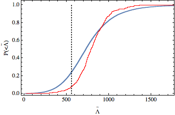
Figure 4: Population measurement enables sharper constraints on NS tides: Cumulative posterior distribution of $\tilde{\Lambda}$ for one of the synthetic sources in our BNS population model. Blue curve shows a single-event analysis, not exploiting information about the mass and spin distribution from other events; red curve shows an analysis based on Eq. (16) that employs our best estimate for the underlying mass and spin distribution, as constrained from the population of events in our BNS synthetic sample.

III.2 BBH mass and (precessing) spin distribution

Quantity	${\mathcal{R}}$	$\alpha_{m}$	$m_{\mathrm{min}}$	$m_{\mathrm{max}}$	$\alpha_{\chi}$	$\beta_{\chi}$	$\sigma_{\chi}$
	${\rm Gpc}^{-3}{\rm yr}$		$M_{\odot}$	$M_{\odot}$
Synthetic population	100	0.8	5	40	1.1	5.5	0.4
Prior range	$[10^{-1},10^{6}]$	$[-5,5]$	$[5,5]$	$[30,195]$	$[10^{-4},10^{4}]$	$[10^{-4},10^{4}]$	$[10^{-2},10^{2}]$
Prior distribution	Log-uniform	Uniform	Uniform	Uniform	Log-uniform	Log-uniform	Log-uniform

Table 1: Synthetic BBH population model: This table shows the parameters of the population model family we adopt to generate and recover a synthetic binary black hole population as described in Sec. III.2. The population is characterized by an overall BBH merger rate ${\cal R}$; a power-law slope $\alpha_{m}$ for the primary mass, between $m_{\rm min}$ and $m_{\rm max}$; a beta distribution for spin magnitude, characterized by the two parameters $\alpha,\beta$ [Eq (10)]; and a characteristic misalignment $\sigma_{\chi}$ for the angle between BH spins and the orbital angular momentum at our reference frequency [Eq. (11)]. This analysis also fixes the maximum allowed total mass $M_{\rm max}$ (i.e., $m_{1}+m_{2}\leq M_{\rm max}$) to $200M_{\odot}$. In this model, both black hole spins are assumed drawn independently from the same distribution. The second row shows the values of these parameters used to generate our synthetic population. The third row shows the range of parameter space we explore when attempting to reproduce our data. The fourth row shows the prior distribution adopted for each parameter, all assumed a priori independent; in this row, “log uniform” implies the prior distribution for any variable $x$ is uniform as a function of $\log x$ [i.e., $p(x)\propto 1/x$]. Note that for simplicity we have assumed the minimum mass is known.

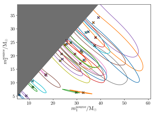
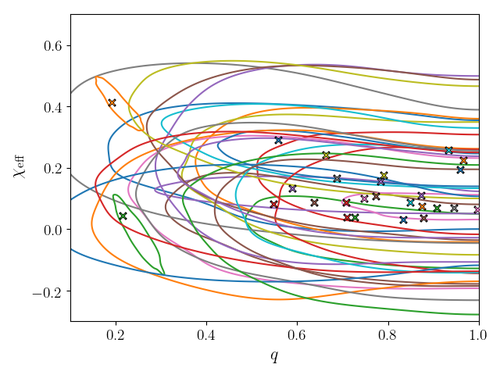
Figure 5: Source information for our synthetic BBH population: For each synthetic signal used in the BH population reconstruction calculation described in Sec. III.2, these two panels show the true injected source-frame parameters (as crosses) and posterior distributions (contours of their 95% highest posterior density regions). Each color corresponds to a different source.

To assess our ability to simultaneously constrain both the mass and spin distribution of binary black holes using GW observations, we constructed a synthetic population drawn from our fiducial BBH population model, with parameters as described in Table 1. Following the procedure described in Appendix B, we drew freely from this population, then selected a subsample based on their relative probability of detection, producing 25 events based on 300 days of synthetic observation at O1 sensitivity. For both the synthetic population and sensitivity model, we approximate $VT$ by neglecting any effects of spin, as a self-consistent leading-order approximation. For each event, we generated 1000 fair draws from a synthetic posterior distribution, using the procedure described in Appendix A. These synthetic or “mock” posterior distributions mimic the effects of full GW parameter inference, but by construction only explicitly constrain the binary chirp mass, mass ratio, and effective spin $\chi_{\mathrm{eff}}$ of each event. Fig. 5 shows the specific source population and synthetic posteriors used in this analysis. Using these synthetic posterior distributions, we apply the population inference procedure described in Sec. II to produce our best estimates for the population parameters responsible for our synthetic observations. As summarized in Table 1, our model has parameters

$$\Lambda\equiv(\mathcal{R},\alpha_{m},m_{\mathrm{min}},m_{\mathrm{max}},\alpha_{\chi},\beta_{\chi},\sigma_{\chi}).$$ (17)

To be consistent with the priors adopted in other work Abbott et al. (2016) (The LIGO Scientific Collaboration and the Virgo Collaboration), we express our results after reweighting to correspond to a Jeffries prior on the rate [$\pi(\mathcal{R})\propto\mathcal{R}^{-1/2}$]. Even with only 25 events drawn from a preferentially low-spin population, our calculations show that GW measurements should strongly constrain the mass and spin distribution of binary black holes

Fig. 6 shows how well we can determine the merger rate versus binary masses, such as the primary mass. Notably and in good agreement with previous work, we find we can strongly constrain the maximum detectable mass in the population Talbot and Thrane (2017); Fishbach and Holz (2017). Following the discussion Sec. II.5, however, we emphasize that while the maximum detectable mass—demarcated by a sharp cutoff in the observed population—is well constrained, the parameters $\mathcal{R}$, $m_{\mathrm{max}}$, $\alpha_{m}$ have a degeneracy: as shown in Fig. 6, a population with extremely few but very massive BHs is hard to rule out, enabling larger $m_{\mathrm{max}}$ to be consistent with our synthetic observations. Additionally and for the first time, we demonstrate how to self-consistently compute both the overall event rate distribution, including Poisson error, while simultaneously constraining the mass distribution. Previous investigations have used specially devised calculations which marginalize over the event rate distribution, producing results that (for a suitable Jeffries prior) are consistent with our results for the marginal mass distribution. As desmonstrated in Fig. 6, to produce a self-consistent rate distribution, due to strong correlations between the event rate and mass distribution, we must simultaneously measure the mass-dependent merger rate in the local universe. Because the correlation between the event rate and mass distribution arises through the expected number of events, we can provide a simple analytic model for the correlation between the mass distribution and event rate, as described in Appendix C.

With 25 events, our population model has enough information to produce strong constraints on the underlying phenomenological distributions, even for parameters such as spin which are weakly constrained by individual measurements. Fig. 7 illustrates how informative these constraints can be about the spin distribution. This figure compares the true marginal distribution of $q,\chi_{\text{eff}}$ for the BH-BH population to our best (posterior predictive) estimate of that distribution. Even with only a few tens of detections, the estimate traces the general structure of the true distribution. In particular, we can clearly and unambiguously identify that a bias in the $\chi_{\text{eff}}$ distribution toward positive values suggests an underlying tendency toward alignment. Of course, our synthetic observations were intentionally drawn from the model family we use to fit it; in general, the underlying astrophysical distribution may have a form outside the model family we adopt, introducing small biases into our interpretation. Nonetheless, our analysis substantially generalizes previous proof-of-concept demonstrations on how well BH measurements can measure BH spin distributions, not being limited to a single spin magnitude, a discrete and restrictive family of orientation distributions, or similar strong prior adopted in previous investigations Stevenson et al. (2017); Vitale et al. (2017b).

Even with only 25 events, we strongly constrain the BH spin distribution, in both magnitude and orientation (Fig. 8). As described in Appendix C in greater quantitative detail, these two constraints are easily understood. For this synthetic analysis, the upper limit on spin follows from the $\chi_{\rm eff}$ distribution of recovered sources. Since our synthetic observations included no events with large $\chi_{\rm eff}$, we can be confident BH spins are not extremely large, since by chance we ought to have found one large value of $\chi_{\rm eff}$ out of $25$, even allowing for uncertainty in how they are oriented. Similarly, because our synthetic population is preferentially aligned ($\sigma=0.4$), the recovered population shown in Fig. 2 has a $\chi_{\rm eff}$ distribution biased toward positive values. Using Eq. (14) for $\overline{\chi}_{\rm eff}$, the bias in $\chi_{\rm eff}$ inevitably implies $\cos\theta$ is preferentially positive and, as described in Appendix C, allows us to limit $\sigma$.

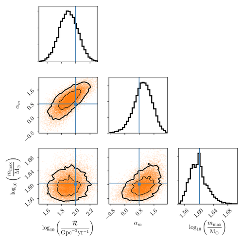
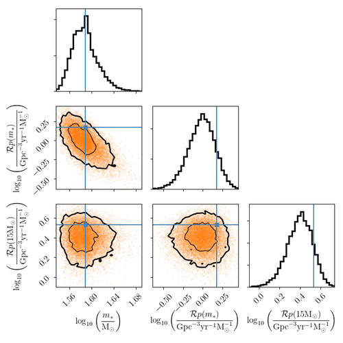
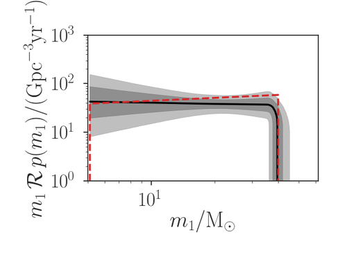
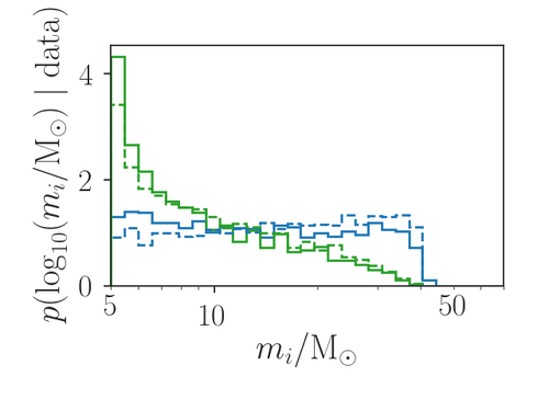
Figure 6: Inferred merger rate versus mass: This figure shows how our estimated merger rate versus mass compares with the known distribution used to generate our synthetic source population. For a more thorough statistical test, see the $P$–$P$ plots in Appendix D. Top left: This group of figures represents the one- and two-dimensional marginal posterior distributions for $\mathcal{R}$, $\alpha_{m}$, and $m_{\mathrm{max}}$, with the true values overlaid as blue crosshairs. Top right: This group of figures represents the one- and two-dimensional marginal posterior distributions for $m_{1}^{*}$, $\mathcal{R}p(m_{1}^{*})$, and $\mathcal{R}p(15\mathrm{M}_{\odot})$, with the true values overlaid as blue crosshairs. Bottom left: In this figure, the red dashed line shows the characteristic merger rate associated with a given mass scale [$m_{1}{\cal R}p(m_{1})$] versus primary mass $m_{1}$. The black line shows the median inferred value, and the two gray shaded regions show the symmetric 68% and 95% credible regions. Bottom right: The solid lines in this figure show our posterior predictive distribution $p(m_{i}|D)$: the best estimate for the probability of a future event being detected having masses $m_{i}$. In this figure, blue and green correspond to the primary and secondary masses. For comparison, the dotted lines show the true astrophysical distribution.

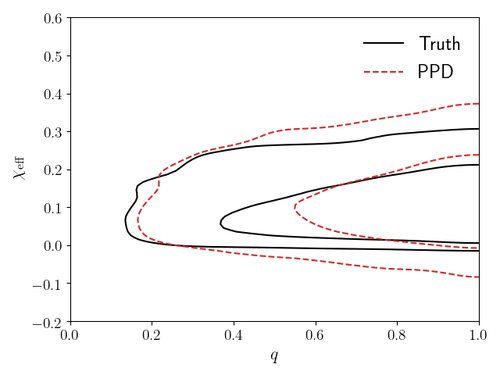
Figure 7: Recovering the true mass ratio and $\chi_{\rm eff}$ distribution: A comparison between the underlying truth (black solid contours) and the inferred posterior predictive (red dashed contours) for the $q$, $\chi_{\text{eff}}$ marginal distribution. The inner (outer) contour for each denotes the 50% (90%) highest probability density credible region.

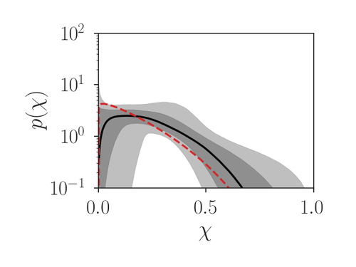
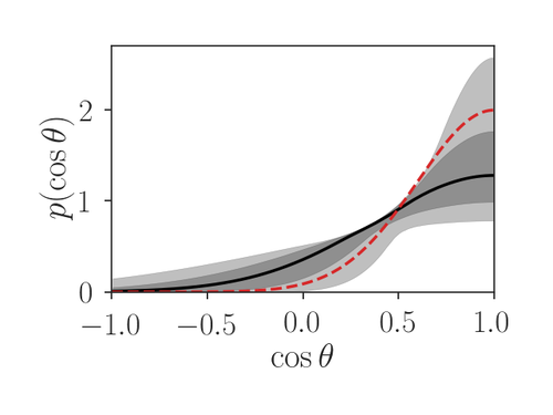
Figure 8: Inferred spin distribution derived from synthetic BBH observations: The top panel shows our inferences about the total BH spin; the bottom panel shows our inferences about BH spin-orbit misalignment. In both panels, the red dashed lines show the underlying distribution, while the black solid lines and shaded regions show the median recovered parameter distribution. To a first approximation, the constraints on spin magnitude and misalignment are as needed for the population model to reproduce the mass and $\chi_{\rm eff}$ distribution of the underlying population as shown in Fig. 7.

In this analysis, we employ conservative synthetic posteriors which assume only the chirp mass, mass ratio, and effective spin can be constrained with GW measurements. Precessing, coalescing binaries can produce a rich symphony of gravitational waves just prior to and during merger, reflecting complex binary dynamics and strong-field multimodal radiation. Given the high expected event rate in ongoing gravitational wave surveys, we expect that future observations will provide clear examples of precessional dynamics, if nature produces them, and that these measurements will allow us to much more sharply constrain the BH spin distribution. However, for massive BH binaries, model systematics complicate attempts to measure BH parameters, including spin. We will conduct full end-to-end calculations with synthetic data and state of the art models in future work.

IV Analysis of reported observational results

To date, five confident binary black hole mergers have been reported: GW150914 Abbott et al. (2016b), GW151226 Abbott et al. (2016a), GW170104 Abbott et al. (2017), GW170608 The LIGO Scientific Collaboration et al. (2017a), and GW170814 The LIGO Scientific Collaboration et al. (2017b) – the latter discovered jointly with the Advanced Virgo instrument Acernese et al. (2015), Additionally, an astrophysically plausible candidate BBH signal has been reported (LVT151012) Abbott et al. (2016) (The LIGO Scientific Collaboration and the Virgo Collaboration). In this section, we describe inferences about the binary black hole population based on reported events, deduced from these reported observations and a simplified model for the network’s search sensitivity. For O1 events, most notably for GW151226, we use full posterior inferences derived from GW data, provided by the LIGO Scientific Collaboration. For O2 events, in lieu of full posterior inferences, we use the procedure described in Appendix A to generate synthetic posterior distributions which closely resemble the reported parameter estimates for mass and $\chi_{\rm eff}$. For simplicity as well as to enable a concrete illustration of our method using real data, we will produce estimates under the (unwarranted) assumption that reported O2 results available to date represent a comprehensive and fair sample of binary black holes seen during LIGO’s O2 observing run. In these estimates, we assume O1 and O2 share a common sensitive volume $V$ as estimated in Sec. II.3, with observing duration $T_{\mathrm{O1}}=48.6\,{\rm days}$ Abbott et al. (2016) (The LIGO Scientific Collaboration and the Virgo Collaboration) and $T_{\mathrm{O2}}=117\,{\rm days}$ The LIGO Scientific Collaboration et al. (2017c). Keeping in mind model systematics such as the omission of a salient feature in the mass distribution can demonstrably strongly bias recovered model parameters Fishbach and Holz (2017); Talbot and Thrane (2018), as well as sample incompleteness for our O2-scale analysis, in Table 2 we provide our inferences about the O1 and O2 population within the context of the fiducial BBH population model described in Sec. III.2. For O2 in particular, we emphasize the simplified $VT$ and non final sample used in that analysis, which is provided solely for illustration and to connect to previously published investigations about O2-scale events Fishbach and Holz (2017); Farr et al. (2017); Wysocki et al. (2018a); applying our methods to final O2 results with real samples and carefully calibrated $VT$ could produce substantially different astrophysical conclusions.

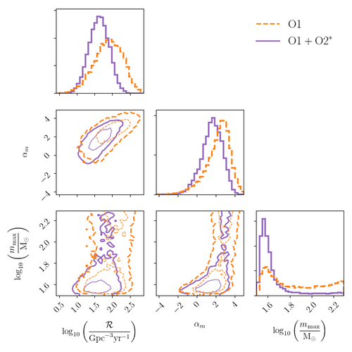
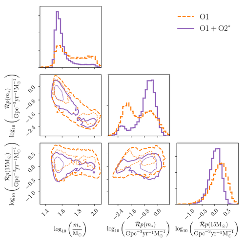
Figure 9: Inferences about astrophysical binary BH mass distribution: Inferences about the merger rate versus mass of coalescing BH-BH binaries, using only O1 observations (dashed orange) and using O1 and reported O2 observations (solid purple), for simplicity assuming the latter represent a comprehensive and fair sample. We apply an asterisk (O2^*) to all O2 results, to highlight the nonfinal sample, simplified sensitivity model $VT$, and mocked-up posteriors used in this proof-of-concept analysis. The panels in this figure follow the format of Fig. 6 for representing one- and two-dimensional marginal posterior distributions.

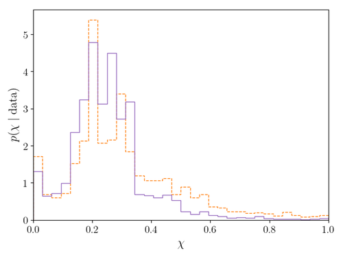
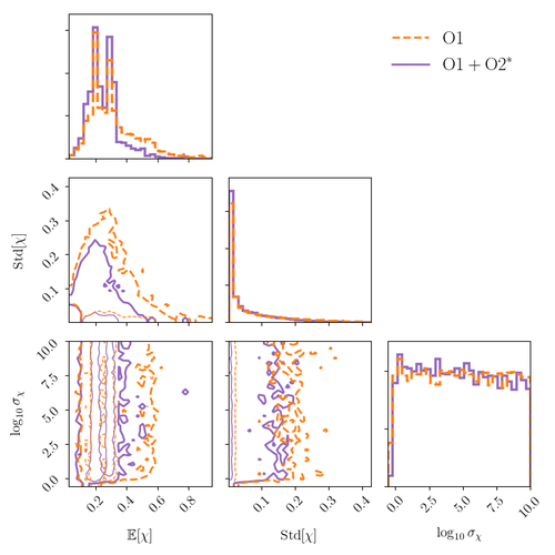
Figure 10: Inferences about astrophysical binary BH spin distribution. Left: Our best estimates for the binary BH spin magnitude distribution (PPD) based on O1 (dashed orange) and O2 (solid purple) observations. We apply an asterisk (O2^*) to all O2 results, to highlight the non final sample, simplified sensitivity model $VT$, and mocked-up posteriors used in this proof-of-concept analysis. Due to the low characteristic spin and within the context of the information used in this analysis, these observations remain uninformative about BH spin-orbit orientations. Right: Our best estimates for the binary BH spin distribution, as expressed using our model hyperparameters, for O1 and O2.

	$\mathcal{R}$	$\alpha_{m}$	$m_{\mathrm{max}}$	$\mathbb{E}[\chi]$	$\mathrm{Std}[\chi]$	$\log_{10}\sigma_{\chi}$	$\chi_{\mathrm{eff}}$	$\chi$
	$\mathrm{Gpc}^{-3}\,\mathrm{yr}^{-1}$		$\mathrm{M}_{\odot}$
O1	$122^{+291}_{-96}$	$2.8^{+1.4}_{-2.5}$	$70^{+110}_{-30}$	$0.28^{+0.31}_{-0.15}$	$0.02^{+0.25}_{-0.02}$	$0.1$–$9.5$	$0.00^{+0.24}_{-0.24}$	$0.03$–$0.68$
O2*	$\cdots$	$1.9^{+1.5}_{-2.0}$	$39^{+98}_{-6}$	$0.24^{+0.21}_{-0.12}$	$0.01^{+0.19}_{-0.01}$	$0.3$–$9.4$	$0.00^{+0.19}_{-0.19}$	$0.04$–$0.49$

Table 2: Inferences about astrophysical binary BH model parameters: This table provides 90% credible intervals for the underlying parameters of our fiducial BBH population model, applied to O1 and reported O2 observations as described in the text. Parameters with clear unimodal structure are represented by their median and the widths of their 90% symmetric probability confidence interval, whereas we only report the 90% upper and lower limits for more poorly constrained parameters. For the spin magnitude distribution, rather than show the (highly correlated) credible intervals for the underlying sampling variables $\alpha_{\chi},\beta_{\chi}$, we instead show credible intervals for the mean value of $\chi$ and the standard deviation of $\chi$. We also show the posterior predictive range of spin magnitudes $\chi$ and effective spins $\chi_{\mathrm{eff}}$. We apply an asterisk (O2^*) to all O2 results, to highlight the nonfinal sample, simplified sensitivity model $VT$, and mocked-up posteriors used in this proof-of-concept analysis.

Fig. 9 shows our best estimates for the merger rate of BH-BH binaries of different masses, inferred within the context of the model described in Table 1 and demonstrated on synthetic data in Sec. III.2. Naturally, we estimate an overall BH-BH merger rate and mass distribution consistent with previously reported results Abbott et al. (2016) (The LIGO Scientific Collaboration and the Virgo Collaboration). Using a Jeffries’ prior for the merger rate, we find $\mathcal{R}=122^{+291}_{-96}\,{\rm Gpc}^{-3}{\rm yr}^{-1}$ based on O1. For O2, we find uncertainty in the event rate is reduced by roughly a factor of 2, both through reduced Poisson error (e.g., six instead of three events) and through sharper constraints on the mass distribution (e.g., reducing prospects for a large maximum mass). Our result for O1 is more conservative (wider) than the power-law result reported previously in Abbott et al. Abbott et al. (2016) (The LIGO Scientific Collaboration and the Virgo Collaboration), $97^{+135}_{-67}\,{\rm Gpc}^{-3}{\rm yr}^{-1}$, because we employ a more flexible model and therefore incorporate more model systematics, notably including the correlation between event rate and mass spectrum and also the impact of the upper mass cutoff. Conversely, if we employ consistent assumptions, we arrive at the same answers previously reported for O1 Abbott et al. (2016) (The LIGO Scientific Collaboration and the Virgo Collaboration). As we adopt a merger rate model that reduces to previously investigated power laws, by design we reproduce the analysis reported in Fishbach and Holz (2017): the events reported during O2 suggest the absence of very massive BHs in the observable population. For this reason our inferences about the mass spectrum exponent $\alpha_{m}$ are considerably wider than prior work which does not take a possible upper mass cutoff into account. Even with the small sample publicly reported so far, our analysis corroborates the analysis in Fishbach and Holz (2017) that O2-scale GW measurements could be weakly informative about the maximum mass of coalescing BHs.

As demonstrated in several previous investigations Farr et al. (2017); Wysocki et al. (2018a), we know that BHs in merging binaries likely have low typical spin. For example, based on the distribution of $\chi_{\rm eff}$, Farr et al. Farr et al. (2017) argued that several members of a discrete array of candidate spin orientations (aligned or isotropic) and magnitude distributions are inconsistent with observations to date, and that BH spins were likely randomly oriented or small. Later, Wysocki and collaborators Wysocki et al. (2018a) demonstrated that, if binary black holes arose from isolated binaries whose spins were weakly misaligned by SN natal kicks, then only relatively small BH natal spins were consistent with observations available at the time. As shown in Fig. 10, with more events available to our analysis, and using much more flexible models, we can draw sharper and more generic conclusions about the BH spin distribution, even using only six reported events. First and foremost, exactly as seen with synthetic data, the absence of large $\chi_{\rm eff}$ allows us to with increasing confidence bound above the fraction of BHs in merging binaries that have large spin. Too, because collectively the observed population distribution of $\chi_{\rm eff}$ remains nearly symmetrically distributed around zero, we can with increasing confidence bound the fraction of binaries that are preferentially aligned and with modest spin. With at least one BH known to have spin (GW151226) and for simplicitly assuming the BH spin and mass distribution are uncorrelated, we are led to weakly disfavor scenarios where BHs are preferentially aligned (i.e., small $\sigma$ is disfavored). We emphasize, however, that this conclusion is driven by the absence of strong support for any spin in all but one binary (GW151226). We would arrive at the same nominal conclusion for a comparable number of random draws from a binary population model with perfectly aligned binaries with small BH spins. Future and more informative observations of BH binaries could significantly alter this conclusion.

V Discussion

In this work, we present concrete examples for how well just a handful of GW measurements can improve our phenomenology of the BH mass and spin distribution. Our examples include real observational data from LIGO’s O1 and (an incomplete sample from) O2 observing run, suggesting current observations could be on the cusp of constraining BH spins and maximum masses. We provide simple estimates to understand how well these parameters have been constrained, allowing the reader to extrapolate to larger sample sizes. For example, in the absence of positive support for spin, the upper limit on BH spin will decrease rapidly, allowing us to place strong upper limits for (or enable discovery of) BH natal spin.

Because each empirical marginal distribution possesses an infinite number of degrees of freedom, any phenomenological parametrization such as our own can quickly be exhausted by the data O’Shaughnessy (2013), particularly when the population must reproduce multiple observational features. In the short run, therefore, we anticipate a fully generic and regularized infinite-dimensional approach will soon be required to adequately reproduce the thousands of events that even the current generation of instruments will discover. A fully generic approach, however, can easily be misled, not least because GW measurements are subject to many subtle strong-field systematics due to model incompleteness. For example, a waveform approximation widely used for rapid parameter inference of binary black holes (IMRPv2 Hannam et al. (2014)) omits astrophysically critical degrees of freedom—the calculation allows for only one precessing spin instead of the two necessary to fully describe the dynamics—and demonstrably has systematic errors large enough to shift posterior distributions for O3-scale events by an appreciable fraction of their statistically expected extent Williamson et al. (2017); Lange et al. (2018). To illustrate the pernicious impact of these systematic biases, we can consider a simple order-of-magnitude estimate: a single quantity, with intrinsic Gaussian distribution of mean $\mu$ and width $\sigma$, being observed multiple times by an apparatus with a (Gaussian, random) measurement error $\Delta x$ and bias $\delta x$. The bias will be important when it influences our best estimate of the average (i.e., when $\delta x\gtrsim\sqrt{\sigma^{2}+\Delta x^{2}}/\sqrt{N}$). Applying this order-of-magnitude approach to GW measurements, we expect that after only a few tens of binary mergers, these modeling systematics will progressively contaminate the interpretation of coalescing binaries, as posterior biases in each event become reflected in biases in the inferred population distribution. Waveform systematics will be even more important because BH spins appear to be small: greater accuracy is needed to separate the secular effects of spin. In this work, when carrying out a full parameter inference, we use the newly developed RIFT parameter inference engine Lange et al. (2018) to produce posteriors. We will discuss the impact of waveform systematics on BH spin misalignment measurements in future work.

VI Conclusions

We have introduced a flexible, ready-to-use, and self-consistent parametric method to estimate the compact binary merger rate as a function of binary parameters, specifically emphasizing mass and spin. Unlike prior work, our procedure self-consistently estimates the merger rate and binary parameter distribution, accounting for statistical sampling error, measurement error, and selection bias. Using this procedure, we show by example that only a handful of NS-NS and BH-BH measurements can enable strong constraints on their respective populations via GW observations alone. Even in the astrophysically likely scenario of small BH spin, we emphasize that just a few measurements will enable sharp constraints on the BH spin distribution. Interpreting current observations, we show that GW measurements are already beginning to place astrophysically interesting constraints on the spin of BHs. We reproduce prior results about the lack of reported BHs at high mass and its implications for the BH mass spectrum. Finally, particularly in our appendix, we explain how to extrapolate toward the measurement prospects available in the very near future.

The procedure described here assumes all sources have been unambiguously resolved from observational data, omitting any treatment of source significance aside from a naive selection bias. Farr et al. Farr et al. (2015) demonstrated and popularized an approach to self-consistently perform the detection and population inference process, estimating the foreground and background distributions simultaneously; see also Loredo (2004); Buchner et al. (2015); Messenger and Veitch (2013). Recently, Gaebel and collaborators Gaebel et al. (2019) developed a concrete procedure to apply this technique to gravitational wave observations. Owing to many deep similarities between our strategies, we anticipate we will shortly incorporate this technique in our own analysis.

The approach described here also employs several strong assumptions about the (lack of) correlations between model parameters. For example, our fiducial BH model assumes the mass-dependent BH merger rate is independent of redshift; that BH masses and spins are completely independent; and that BH spin misalignment and spin magnitudes are likewise uncorrelated. We will explore more physically motivated correlations in future work.

In the long run, phenomenology is only as sound as the underlying parametrization. Previous analyses have repeatedly shown that adopting an overly restrictive model will produce biased results, as demonstrated by Fishbach et al (with the maximum mass) Fishbach and Holz (2017) and Talbot et al Talbot and Thrane (2018) (with the shape of the maximum mass cutoff). With sufficient data, a suitably regularized infinite-dimensional parametrization will make unintended systematic biases less frequent. Mature methods for infinite-dimensional or nonparametric inference exist Gelman et al. (2013); Orbanz and Teh (2010); Ghosal and van der Vaart (2017), beginning with simple infinite-dimensional parametrizations plus smoothing priors or with Gaussian processes Rasmussen and Williams (2006). Early investigations have applied nonparametric methods to GW population estimates Wysocki (2017); Mandel et al. (2017). However, because the GW signal is so rich, many parameters can be measured for each event, several of which are believed to be correlated in most astrophysical formation scenarios. These correlations should be more sharply identified with strong theoretical priors for the immediate future.

Finally, several technical improvements can make this approach faster and more robust. For example, we can perform inference on all events simultaneously, using direct estimates of the likelihood $\ell(\lambda)$ naturally reported by RIFT, to ensure any population inferences are not limited by the compact support of fiducial priors. Using accelerated general-purpose inference engines, we expect to dramatically accelerate the speed with which our population inferences are provided, with a long-term goal of enabling low-latency population-informed identification and classification of candidate sources.

Appendix A Mock posterior populations precessing binaries: Aligned Fisher matrix approach

We test our code using synthetic or “mock” posterior distributions for binary black hole parameters, designed to mimic the results of full end-to-end Bayesian inference on synthetic data. For the mock BBH posterior distributions constructed in this work, we adopt a very simple approximation, motivated by decades of experience suggesting that for short BBH signals the likelihood for gravitational wave signals is nearly Gaussian in three coordinates ($\mathcal{M}_{\text{c}},\eta,\chi_{\rm eff}$) and does not strongly constrain any other degrees of freedom. Specifically, if $\lambda_{0}$ are the true binary parameters and $\rho$ is the true network signal amplitude; if $\Gamma_{ab}=\left\langle\partial_{a}h|\partial_{b}h\right\rangle$ is the Fisher matrix for the binary parameters $\lambda$, evaluated at $\lambda=\lambda_{0}$ and for a signal amplitude $\rho$ using a fiducial detector power spetcrum; and if $p(\lambda)$ is the prior distribution on $\lambda$, then we approximate the posterior distribution by a distribution proportional to

$$e^{-\Gamma_{ab}(\lambda-\lambda_{*})_{a}(\lambda-\lambda_{*})_{b}}p_{\rm ref}(\lambda)$$ (18)

where $\lambda_{*}$ is a fixed random realization from a normal distribution with mean $\lambda_{0}$ and covariance matrix $\Gamma^{-1}$. We generate samples from this distribution via Monte Carlo techniques. We evaluate the approximate Fisher matrix $\Gamma$ using the effective Fisher technique O’Shaughnessy et al. (2014); Cho et al. (2013); Cho and Lee (2014), applied to a nonprecessing binary waveform model assigned the same values of $\mathcal{M}_{\text{c}},\eta,\chi_{\rm eff}$ (i.e., via $\chi_{1,z}=\chi_{2,z}=\chi_{\rm eff}$).

This approximate posterior distribution has several distinct advantages. First and foremost, it captures in $\Gamma_{ab}$ the strong, parameter-dependent, and well-understood correlations between the variables that most significantly impact the GW inspiral signal, while simultaneously populating all intrinsic binary parameters. For example, it captures the shape of the posterior distribution in mass ratio and spin while correctly accounting for parameter boundary effects, as described in Ng et al. (2018). Second, it accounts via $\lambda_{*}$ for the effect of random noise realizations, which impact the best-fitting parameters associated with each set of synthetic data. By including an explicit prior $p_{\rm ref}(\lambda)$, it allows us to carefully adopt fiducial prior assumptions, which have a substantial impact on inferred binary masses and spins.

A ready-to-use implementation of this algorithm is available.

For simplicity, in this implementation, no cosmological effects are applied. If used unaltered, this approximate posterior applies either if cosmological redshift effects are small compared to the width of the distribution in mass (i.e., bias is small compared to the statistical uncertainty) or if these ambiguity distributions are used to approximate the source-frame ambiguity function. Cosmological effects dominate the accuracy to which a binary neutron star’s chirp mass can be measured; to be used in such a scenario, this approximation must be refined to reflect the significant impact of the sources’ unknown redshift.

Appendix B Mock populations

To generate a synthetic population of events, we employ the following procedure. Using O1 sensitivity, and a detection criterion of $\rho>8$ in a single interferometer, we used our estimate of $V$ and a fiducial observation time $T$ to compute the expected number of events $\mu$. Using the Poisson distribution, we select a total number of events $N$ to observe. We assumed each detected binary had a network SNR drawn from a power law $p(\rho_{\mathrm{network}})\propto\rho_{\mathrm{network}}^{-4}$, with a lower cutoff of $12$ (roughly corresponds to $8$ in two detectors).

Appendix C Overview of key phenomenological constraints

C.1 How well can we measure distribution hyperparameters?

Classical frequentist statistical methods provide a quick way to assess how rapidly observations will constrain model hyperparameters. For example, the sample mean of maximum likelihood estimators converges rapidly to the true mean, and (to a first approximation) the sample variance is approximately $\chi^{2}$ distributed. Thus, by adopting the mean and variance of our underlying distributions as coordinates on the space $\Lambda$ of hyperparameters, we can estimate how efficiently observations will constrain them. For example, if we account for measurement error, we can measure the mean spin to an accuracy $\sqrt{V(\chi)+\sigma_{\chi}^{2}}/\sqrt{N}$ where $V(\chi)$ is the variance of the spin magnitude distribution and $\sigma_{\chi}$ is the typical spin measurement accuracy for the mass range of interest [typically $\mathcal{O}(0.3)$]. Because of sharp cutoffs, the maximum and minimum masses have a qualitatively different behavior; see, e.g., Amari and Nagaoka (2007). Both the maximum and minimum masses are best estimated using the most extreme individual event, with an accuracy converging as $1/N$. In our context—the power-law mass distribution—the accuracy with which these maximum masses can be determined scales directly with the number of events in a given region. We therefore expect the maximum mass can be determined to an accuracy of order $m_{\rm max}/N$; the appropriate scale factor can be calibrated to detailed analyses of the kind performed in Sec. III. Similarly, as described below in Appendix C.2, we can use the observed range of $\chi_{\rm eff}$ to constrain spin magnitudes and misalignments.

While providing a useful order-of-magnitude estimate into how well we can measure distribution parameters, the simple estimates above become cumbersome when trying to capture correlations between our phenomenological parameters, notably the event rate and mass distribution. Following O’Shaughnessy (2013), we assess how well we can distinguish model hyperparameters from the (expected) log-likelihood as a function of model hyperparameters $\Lambda$ of

$${\left\langle\ln{\cal L}\right\rangle}=-\mu_{*}+\mu_{*}{\left\langle\ln\int d\lambda p(d|\lambda)Rp(\lambda|\Lambda)\right\rangle}_{*}$$ (19)

where the expectation is performed relative to some reference model characterized by parameters $\Lambda_{*}$ such that $p_{*}(\lambda)\equiv p(\lambda|\Lambda_{*})$ and $\mu_{*}=\mu(\Lambda_{*})$. Rather than work in full generality, we perform a Taylor series expansion of the likelihood around the local maximum, characterizing the second order term by its inverse covariance or Fisher matrix $\Gamma_{ab}$

$${\left\langle\ln{\cal L}\right\rangle}\simeq\ln{\cal L}_{*}-\frac{1}{2}\Gamma_{\alpha\beta}(\Lambda-\Lambda_{*})_{\alpha}(\Lambda-\Lambda_{*})_{\beta}$$ (20)

If $\gamma_{k}$ are eigenvalues of $\Gamma$, then hyperparameters can be measured to an accuracy $1/\sqrt{\gamma_{k}}$, which scales as $1/\sqrt{N}$ for $N$ the number of observed events.

We first illustrate this technique in the idealized case of zero measurement error, following previous work O’Shaughnessy (2013) which characterized differences between two distributions $q,p$ using the KL divergence $D_{\mathrm{KL}}(p|q)\equiv\int p(x)\ln[p(x)/q(x)]\mathrm{d}x$. The marginalized log likelihood only depends on model hyperparameters $\Lambda$ through the KL divergence between our proposed model $\mu,p$ (which depends on $\Lambda$) and the reference model $\mu_{*},p_{*}$ (which does not):

$${\left\langle\ln{\cal L}\right\rangle}=-D_{\mathrm{KL}}(\mu_{*}|\mu)-\mu_{*}D_{\mathrm{KL}}(p_{*}|p)+\text{const.}$$ (21)

As a result, the Fisher matrix has two model-dependent terms, each reflecting second derivatives of $D_{\mathrm{KL}}$ with respect to model parameters:

$$\Gamma_{\alpha\beta}^{(zero)}=\Gamma_{\alpha,\beta}^{(\mu)}+\mu_{*}\Gamma_{\alpha\beta}^{(p)}$$ (22)

where the first term arises from differences in the observed number; where the second term reflects differences in shape; and where we use the fact that $D_{\mathrm{KL}}$ has a local minimum (of 0) when the two distributions are equal to eliminate cross terms. Thus, we can evaluate the Fisher matrix simply by computing KL divergences and carrying out the necessary derivatives. For example, for the mass power-law model with fixed mass range, $p(m|\alpha)=C(\alpha,m_{+},m_{-})m_{1}^{-\alpha}/(m_{1}-m_{-})$, the KL divergence $D_{\mathrm{KL}}(p_{*},p)$ becomes

$$D_{\mathrm{KL}}(\alpha_{*}|\alpha) \equiv\int p(x|\alpha_{*})\ln p(x|\alpha_{*})/p(x|\alpha)$$ (23)

$$=(\alpha-\alpha_{*}){\left\langle\ln x\right\rangle}_{\alpha_{*}}+\ln C(\alpha_{*})/C(\alpha)$$ (24)

where the conditional average is ${\left\langle f\right\rangle}_{\alpha}\equiv\int dxf(x)p(x|\alpha)$. In this expression, only the last term $-\ln C(\alpha)$ does not cancel in $\partial_{\alpha}^{2}D_{\mathrm{KL}}(\alpha_{*}|\alpha)$.

Again using the same concrete power-law example, we next use this technique to show how, because $\mu$ [Eq. (6)] and the mass distribution can be independently constrained, the “overall event rate” ${\cal R}$ and the mass distribution are correlated. Representing $\mu=e^{X}$, the second derivative of $D_{\mathrm{KL}}(\mu_{*}|\mu)$ becomes O’Shaughnessy (2013)

$$D_{KL}\simeq\frac{1}{2}\mu_{*}(\partial_{a}X)(\partial_{b}X)(\Lambda-\Lambda_{*})_{a}(\Lambda-\Lambda_{*})_{b}$$ (25)

For the power-law model described above, the only two derivatives needed are $\partial_{\ln R}X=1$ and $\partial_{\alpha}X=\partial_{\alpha}\ln{\left\langle VT\right\rangle}_{\alpha}$, the latter of which can be well approximated by $-1$. This term introduces correlations between the rate variable ($\ln{\cal R}$) and shape ($\alpha$). Conversely, using coordinates $\mu$ and $\alpha$ to characterize the observed population, by construction our inferred posterior distribution on the total number and mass distribution are uncorrelated.

Roughly speaking, the effects of measurement error add in quadrature in the Fisher matrix:

$$\Gamma=\Gamma^{(\mathrm{zero})}+\Gamma^{(\mathrm{measure})}$$ (26)

We can therefore refine the estimates provided above to incorporate simple estimates of GW measurement errors and their correlations. For the simple power-law estimate described above, however, these measurement errors are relatively small compared to the range of the distribution, unless $\alpha$ is very large.

In the above order-of-magnitude discussion, we have not accounted for parameter-dependent selection bias. To a good first approximation, GW selection bias enters only through the masses, roughly as the (chirp) mass to a power. We can therefore treat the observed population as a (different) power law, which observations constrain to an accuracy loosely characterized by the analysis above.

Therefore, for the power-law mass distribution, we expect the posterior distribution of (log) rate and powerlaw exponent will be correlated and follow a Gaussian distribution characterized by the inverse covariance

$$\Gamma\simeq\mu\begin{bmatrix}1&-1\\ -1&1+2\partial_{\alpha}^{2}\ln C(\alpha)\end{bmatrix}$$ (27)

relative to the coordinates $(\ln{\cal R},\alpha)$, if we adopt a uniform prior on $\alpha$ and $\ln R$. This expression captures the correlations between the rate and mass ratio seen in our inferences, when only varying the total event rate and mass ratio.

C.2 Semianalytic model for constraints on the spin magnitude and misalignment distribution

In this paper, for the purposes of illustration and as a leading-order approximation suitable for the BH-BH binaries reported to date, we adopt three simplifying approximations: that the sensitive volume depends weakly on spin; that GW measurements will only constrain $\chi_{\rm eff}$; and that the underlying mass and spin distributions of BH-BH binaries are uncorrelated. In this framework of approximations, only $\chi_{\rm eff}$ measurements and hence the underlying $\chi_{\rm eff}$ distribution of the population determines how well we can distinguish between population models via spin measurements. Within this framework, we can simply and largely analytically estimate how much information we gain about the BH spin distribution from repeated measurements.

In our synthetic model (and nature) where BH spins appear to be small, the first few measurements will principally inform our upper limit on the BH spin distribution, via the absence of observations consistent with large $\chi_{\rm eff}$. For example, in our synthetic model, the 90% upper limit expected in 25 events is $\chi_{\rm eff}<0.31$; for our inferred posterior predictive distribution based on all published events, it is $0.19$. In Fig. 11, we use a simple toy model to illustrate how upper limits loosely inform our estimates of the BH spin distribution. In this model, we assume each BH in a binary has a random spin magnitude drawn from a uniform distribution between 0 and $\chi_{\rm max}$, randomly (isotropically) oriented, for binaries with a random mass ratio uniformly drawn between $0.1$ and $1$. This figure shows the cumulative distribution of $\chi_{\rm eff}$ implied by these assumptions, for different choices of $\chi_{\rm max}$. These cumulative distributions are well approximated by analytic expressions for the cumulative distribution of $\chi_{1,z}$ and $\chi_{\rm eff}$ under these assumptions; see Lange et al. (2018) for concrete expressions. For comparison, the vertical shaded regions show the largest values of $\chi_{\rm eff}$ which have significant support in our synthetic sample ($\chi_{\rm eff}\lesssim 0.5$), consistent with the largest plausible spins reported for O1 and O2 events. The lack of support for large $\chi_{\rm eff}$ in any observation to date strongly suggests that BH spins cannot be large. Conversely, an observation of a binary with $\chi_{\rm eff}$ bounded below by $\epsilon$ (e.g., GW151226) implies that a significant fraction of BH spins must be greater than of order $\epsilon$.

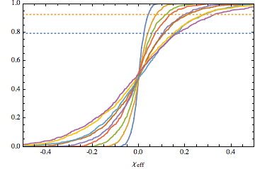
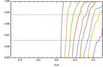
Figure 11: Why $\chi_{\rm eff}$ measurements constrain the maximum spin: cumulative distribution function for $\chi_{\rm eff}$ for toy models with isotropic spins and uniform spin magnitude distributions limited by $0.1,0.2,0.3,\ldots$. In the top panel, the vertical lines, corresponding to $0.5^{1/3}$ and $0.5^{1/25}$, indicate the locus of points in each cumulative distribution function we can begin to constrain with the absence of events above $X$ with $3$ and 25 events, respectively. In the bottom panel, the lines have been changed to $0.9^{1/3}$ and $0.9^{1/25}$, respectively.

We emphasize that we provide these estimates (and perform our calculation within these underlying approximations) to produce a conservative, well-understood benchmark for how well the BH spin distribution can be constrained with present and future GW measurements. Real GW measurements, particularly of low-mass or closer and therefore higher-amplitude BH-BH mergers, will provide additional direct constraints on the other spin degrees of freedom.

Appendix D End-to-end tests of population hyperparameter recovery: $P$–$P$ plots

A standard technique to test Bayesian parameter inference codes is a probability-probability or $P$–$P$ plot. We employ this test both on our population inference engine and on the procedure for making synthetic observations. For our population inference code, we generate $k=1\cdots 1000$ synthetic BBH populations, each a fair draw from a set of population hyperparameters controlling the rate, mass and spin distribution. For each synthetic population, we generate one random observing run with O1 LIGO sensitivity and $T=300\,\mathrm{days}$ coincident observing time, by computing the expected number of detections $\mu$ [Eq. 6] and taking one random Poisson draw $p(n_{k})\propto e^{-\mu}\mu^{n_{k}}/n_{k}!$. We take $n_{k}$ detection-weighted binaries, generating parameter estimates according to the procedure in Appendix B. We then apply our population parameter inference code to generate posterior distributions on the population hyperparameters $\Lambda$, and from that one-dimensional marginal cumulative distributions $\hat{P}_{k,i}(\Lambda_{i})$, for each parameter $\Lambda_{i}$. It should be noted here that we used as our prior the same distribution that these population hyperparameters were drawn from, as anything else would produce biases. Using the true hyperparameter values $\Lambda^{*}_{k,i}$, we generate a single number for each hyperparameter $\hat{P}_{k,i}(\Lambda^{*}_{k,i})$. A $P$–$P$ plot is the cumulative distribution of these $\hat{P}_{k,i}(\Lambda^{*}_{k,i})$. If the code is behaving correctly, these should be uniformly distributed from 0 to 1: the plot should be diagonal. The top panel of Fig. 12 shows the $P$–$P$ plots for each of our model hyperparameters.

In addition to our population inference code, we made $P$–$P$ plots for our synthetic parameter estimation code, described in Appendix B, as our population inference tests make use of it. Here we generated $k=1\cdots 1000$ synthetic BBH signals, drawing true values from the prior we used for measuring the posteriors. We repeated the same process just described, making posterior distributions on the intrinsic parameters $\lambda$, and evaluating the marginal cumulative distribution functions at the true values $\lambda^{*}_{k}$. $P$–$P$ plots for some representations of the intrinsic parameters are shown in the bottom panel of Fig. 12.

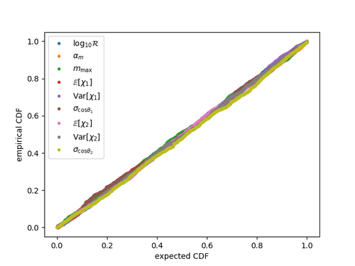
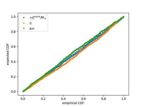
Figure 12: $P$–$P$ plots for hyperparameter recovery. Top (bottom) panel shows the $P$–$P$ plot for population (single synthetic event) inferences.

References

- Abbott et al. (2015) (The LIGO Scientific Collaboration) B. Abbott et al. (The LIGO Scientific Collaboration), CQG 32, 074001 (2015), arXiv:1411.4547 [gr-qc] .
- Accadia and et al (2012) T. Accadia and et al, Journal of Instrumentation 7, P03012 (2012).
- Acernese et al. (2015) F. Acernese et al. (VIRGO), CQG 32, 024001 (2015), arXiv:1408.3978 [gr-qc] .
- Abbott et al. (2016) (The LIGO Scientific Collaboration and the Virgo Collaboration) B. Abbott et al. (The LIGO Scientific Collaboration and the Virgo Collaboration), ApJ 833, L1 (2016), arXiv:1602.03842 [astro-ph.HE] .
- Abbott et al. (2016) (The LIGO Scientific Collaboration and the Virgo Collaboration) B. Abbott et al. (The LIGO Scientific Collaboration and the Virgo Collaboration), \prx 6, 041015 (2016), arXiv:1606.04856 .
- Abbott et al. (2016a) (The LIGO Scientific Collaboration and the Virgo Collaboration) B. Abbott et al. (The LIGO Scientific Collaboration and the Virgo Collaboration), ApJ 818, L22 (2016a), arXiv:1602.03846 [astro-ph.HE] .
- Mandel and de Mink (2016) I. Mandel and S. E. de Mink, MNRAS 458, 2634 (2016), arXiv:1601.00007 [astro-ph.HE] .
- Marchant et al. (2016) P. Marchant, N. Langer, P. Podsiadlowski, T. Tauris, and T. Moriya, A&A 588, A50 (2016), arXiv:1601.03718 [astro-ph.SR] .
- Rodriguez et al. (2016a) C. L. Rodriguez, C.-J. Haster, S. Chatterjee, V. Kalogera, and F. A. Rasio, ApJ 824, L8 (2016a), arXiv:1604.04254 [astro-ph.HE] .
- Bird et al. (2016) S. Bird, I. Cholis, J. B. Muñoz, Y. Ali-Haïmoud, M. Kamionkowski, E. D. Kovetz, A. Raccanelli, and A. G. Riess, Physical Review Letters 116, 201301 (2016), arXiv:1603.00464 .
- Kushnir et al. (2016) D. Kushnir, M. Zaldarriaga, J. A. Kollmeier, and R. Waldman, MNRAS 462, 844 (2016), arXiv:1605.03839 [astro-ph.HE] .
- Lamberts et al. (2016) A. Lamberts, S. Garrison-Kimmel, D. R. Clausen, and P. F. Hopkins, MNRAS 463, L31 (2016), arXiv:1605.08783 [astro-ph.HE] .
- Dvorkin et al. (2016) I. Dvorkin, E. Vangioni, J. Silk, J.-P. Uzan, and K. A. Olive, MNRAS 461, 3877 (2016), arXiv:1604.04288 [astro-ph.HE] .
- Abbott et al. (2016b) (The LIGO Scientific Collaboration and the Virgo Collaboration) B. Abbott et al. (The LIGO Scientific Collaboration and the Virgo Collaboration), Phys. Rev. Lett. 116, 131102 (2016b).
- Barack et al. (2018) L. Barack, V. Cardoso, S. Nissanke, T. P. Sotiriou, A. Askar, C. Belczynski, G. Bertone, E. Bon, and et al., ArXiv e-prints (2018), arXiv:1806.05195 [gr-qc] .
- Wysocki et al. (2018a) D. Wysocki, D. Gerosa, R. O’Shaughnessy, K. Belczynski, W. Gladysz, E. Berti, M. Kesden, and D. E. Holz, Phys. Rev. D 97, 043014 (2018a), arXiv:1709.01943 [astro-ph.HE] .
- Mandel and O’Shaughnessy (2010) I. Mandel and R. O’Shaughnessy, Classical and Quantum Gravity 27, 114007 (2010), arXiv:0912.1074 [astro-ph.HE] .
- Rodriguez et al. (2016b) C. L. Rodriguez, M. Zevin, C. Pankow, V. Kalogera, and F. A. Rasio, ApJ 832, L2 (2016b), arXiv:1609.05916 [astro-ph.HE] .
- Breivik et al. (2016) K. Breivik, C. L. Rodriguez, S. L. Larson, V. Kalogera, and F. A. Rasio, ApJ 830, L18 (2016), arXiv:1606.09558 .
- Nishizawa et al. (2016) A. Nishizawa, E. Berti, A. Klein, and A. Sesana, Phys. Rev. D 94, 064020 (2016), arXiv:1605.01341 [gr-qc] .
- Fishbach and Holz (2017) M. Fishbach and D. E. Holz, ApJ 851, L25 (2017), arXiv:1709.08584 [astro-ph.HE] .
- Talbot and Thrane (2018) C. Talbot and E. Thrane, ApJ 856, 173 (2018), arXiv:1801.02699 [astro-ph.HE] .
- O’Shaughnessy (2013) R. O’Shaughnessy, Phys. Rev. D 88, 084061 (2013), arXiv:1204.3117 [astro-ph.CO] .
- Stevenson et al. (2015) S. Stevenson, F. Ohme, and S. Fairhurst, ApJ 810, 58 (2015), arXiv:1504.07802 [astro-ph.HE] .
- Belczynski et al. (2016a) K. Belczynski, D. E. Holz, T. Bulik, and R. O’Shaughnessy, Nature 534, 512 (2016a), arXiv:1602.04531 [astro-ph.HE] .
- Zevin et al. (2017) M. Zevin, C. Pankow, C. L. Rodriguez, L. Sampson, E. Chase, V. Kalogera, and F. A. Rasio, ApJ 846, 82 (2017), arXiv:1704.07379 [astro-ph.HE] .
- Barrett et al. (2018) J. W. Barrett, S. M. Gaebel, C. J. Neijssel, A. Vigna-Gómez, S. Stevenson, C. P. L. Berry, W. M. Farr, and I. Mandel, MNRAS (2018), 10.1093/mnras/sty908, arXiv:1711.06287 [astro-ph.HE] .
- Miyamoto et al. (2017) A. Miyamoto, T. Kinugawa, T. Nakamura, and N. Kanda, Phys. Rev. D 96, 064025 (2017), arXiv:1709.08437 [astro-ph.HE] .
- Wysocki (2017) D. Wysocki, ArXiv e-prints (2017), arXiv:1712.02643 [gr-qc] .
- Mandel et al. (2017) I. Mandel, W. M. Farr, A. Colonna, S. Stevenson, P. Tiňo, and J. Veitch, MNRAS 465, 3254 (2017), arXiv:1608.08223 [astro-ph.HE] .
- Kovetz et al. (2017) E. D. Kovetz, I. Cholis, P. C. Breysse, and M. Kamionkowski, Phys. Rev. D 95, 103010 (2017), arXiv:1611.01157 .
- Talbot and Thrane (2017) C. Talbot and E. Thrane, Phys. Rev. D 96, 023012 (2017), arXiv:1704.08370 [astro-ph.HE] .
- Farr et al. (2017) W. M. Farr, S. Stevenson, M. C. Miller, I. Mandel, B. Farr, and A. Vecchio, Nature 548, 426 (2017), arXiv:1706.01385 [astro-ph.HE] .
- Gerosa and Berti (2017) D. Gerosa and E. Berti, Phys. Rev. D 95, 124046 (2017), arXiv:1703.06223 [gr-qc] .
- Fishbach et al. (2017) M. Fishbach, D. E. Holz, and B. Farr, ApJ 840, L24 (2017), arXiv:1703.06869 [astro-ph.HE] .
- Stevenson et al. (2017) S. Stevenson, C. P. L. Berry, and I. Mandel, MNRAS 471, 2801 (2017), arXiv:1703.06873 [astro-ph.HE] .
- Vitale et al. (2017a) S. Vitale, R. Lynch, V. Raymond, R. Sturani, J. Veitch, and P. Graff, Phys. Rev. D 95, 064053 (2017a), arXiv:1611.01122 [gr-qc] .
- Farr et al. (2018) B. Farr, D. E. Holz, and W. M. Farr, ApJ 854, L9 (2018), arXiv:1709.07896 [astro-ph.HE] .
- Vitale et al. (2017b) S. Vitale, R. Lynch, R. Sturani, and P. Graff, Classical and Quantum Gravity 34, 03LT01 (2017b), arXiv:1503.04307 [gr-qc] .
- O’Shaughnessy et al. (2017) R. O’Shaughnessy, D. Gerosa, and D. Wysocki, Phys. Rev. Lett. 119, 011101 (2017).
- Kalogera (2000) V. Kalogera, ApJ 541, 319 (2000), astro-ph/9911417 .
- Belczynski et al. (2010) K. Belczynski, M. Dominik, T. Bulik, R. O’Shaughnessy, C. L. Fryer, and D. E. Holz, ApJ 715, L138 (2010), arXiv:1004.0386 [astro-ph.HE] .
- O’Shaughnessy et al. (2012) R. O’Shaughnessy, R. Kopparapu, and K. Belczynski, CQG 29, 145011 (2012), arXiv:0812.0591 .
- Dominik et al. (2012) M. Dominik, K. Belczynski, C. Fryer, D. E. Holz, E. Berti, T. Bulik, I. Mandel, and R. O’Shaughnessy, ApJ 759, 52 (2012), arXiv:1202.4901 [astro-ph.HE] .
- Wysocki et al. (2018b) D. Wysocki, D. Gerosa, R. O’Shaughnessy, K. Belczynski, and et al, Phys. Rev. D 97, 043014 (2018b), arXiv:1709.01943 [astro-ph.HE] .
- Damour (2001) T. Damour, Phys. Rev. D 64, 124013 (2001), gr-qc/0103018 .
- Racine (2008) É. Racine, Phys. Rev. D 78, 044021 (2008), arXiv:0803.1820 [gr-qc] .
- Ajith et al. (2011) P. Ajith, M. Hannam, S. Husa, Y. Chen, B. Brügmann, N. Dorband, D. Müller, F. Ohme, D. Pollney, C. Reisswig, L. Santamaría, and J. Seiler, Physical Review Letters 106, 241101 (2011), arXiv:0909.2867 [gr-qc] .
- Lange et al. (2018) J. Lange, R. O’Shaughnessy, and M. Rizzo, arXiv e-prints , arXiv:1805.10457 (2018), arXiv:1805.10457 [gr-qc] .
- Abbott et al. (2016c) (The LIGO Scientific Collaboration and the Virgo Collaboration) B. Abbott et al. (The LIGO Scientific Collaboration and the Virgo Collaboration), Phys. Rev. Lett. 116, 241102 (2016c).
- Veitch et al. (2015) J. Veitch, V. Raymond, B. Farr, W. M. Farr, P. Graff, S. Vitale, B. Aylott, K. Blackburn, N. Christensen, M. Coughlin, W. D. Pozzo, F. Feroz, J. Gair, C. Haster, V. Kalogera, T. Littenberg, I. Mandel, R. O’Shaughnessy, M. Pitkin, C. Rodriguez, C. Röver, T. Sidery, R. Smith, M. V. D. Sluys, A. Vecchio, W. Vousden, and L. Wade, Phys. Rev. D 91, 042003 (2015).
- Abbott et al. (2016d) (The LIGO Scientific Collaboration and the Virgo Collaboration) B. Abbott et al. (The LIGO Scientific Collaboration and the Virgo Collaboration), Phys. Rev. D 94, 064035 (2016d).
- Cutler and Flanagan (1994) C. Cutler and É. E. Flanagan, Phys. Rev. D 49, 2658 (1994), gr-qc/9402014 .
- Poisson and Will (1995) E. Poisson and C. M. Will, Phys. Rev. D 52, 848 (1995).
- Cho et al. (2013) H. Cho, E. Ochsner, R. O’Shaughnessy, C. Kim, and C. Lee, Phys. Rev. D 87, 02400 (2013), arXiv:1209.4494 .
- Goodman and Weare (2010) J. Goodman and J. Weare, Commun. Appl. Math. Comput. Sci. 5, 65 (2010).
- Foreman-Mackey et al. (2013) D. Foreman-Mackey, D. W. Hogg, D. Lang, and J. Goodman, PASP 125, 306 (2013), arXiv:1202.3665 [astro-ph.IM] .
- Abadie et al (2010) (The LIGO Scientific Collaboration and the Virgo collaboration) J. Abadie et al (The LIGO Scientific Collaboration and the Virgo collaboration), CQG 27, 173001 (2010), arXiv:1003.2480 [astro-ph.HE] .
- Finn and Chernoff (1993) L. S. Finn and D. F. Chernoff, Phys. Rev. D 47, 2198 (1993), gr-qc/9301003 .
- O’Shaughnessy et al. (2010a) R. O’Shaughnessy, V. Kalogera, and K. Belczynski, ApJ 716, 615 (2010a), arXiv:0908.3635 .
- Dominik et al. (2015) M. Dominik, E. Berti, R. O’Shaughnessy, I. Mandel, K. Belczynski, C. Fryer, D. E. Holz, T. Bulik, and F. Pannarale, ApJ 806, 263 (2015), arXiv:1405.7016 [astro-ph.HE] .
- Husa et al. (2016) S. Husa, S. Khan, M. Hannam, M. Pürrer, F. Ohme, X. J. Forteza, and A. Bohé, Phys. Rev. D 93, 044006 (2016), arXiv:1508.07250 [gr-qc] .
- Khan et al. (2016) S. Khan, S. Husa, M. Hannam, F. Ohme, M. Pürrer, X. J. Forteza, and A. Bohé, Phys. Rev. D 93, 044007 (2016), arXiv:1508.07253 [gr-qc] .
- Brown et al. (2012) D. A. Brown, A. Lundgren, and R. O’Shaughnessy, Phys. Rev. D 86, 064020 (2012), arXiv:1203.6060 [gr-qc] .
- O’Shaughnessy et al. (2010b) R. O’Shaughnessy, B. Vaishnav, J. Healy, and D. Shoemaker, Phys. Rev. D 82, 104006 (2010b), arXiv:1007.4213 [gr-qc] .
- Biswas et al. (2009) R. Biswas, P. R. Brady, J. D. E. Creighton, and S. Fairhurst, Classical and Quantum Gravity 26, 175009 (2009), arXiv:0710.0465 [gr-qc] .
- Tiwari (2018) V. Tiwari, Classical and Quantum Gravity 35, 145009 (2018), arXiv:1712.00482 [astro-ph.HE] .
- Christian et al. (2018) P. Christian, P. Mocz, and A. Loeb, ApJ 858, L8 (2018), arXiv:1803.07094 [astro-ph.HE] .
- Fraley (1968) G. S. Fraley, Ap&SS 2, 96 (1968).
- Fryer et al. (2001) C. L. Fryer, S. E. Woosley, and A. Heger, ApJ 550, 372 (2001), astro-ph/0007176 .
- Woosley et al. (2002) S. E. Woosley, A. Heger, and T. A. Weaver, Reviews of Modern Physics 74, 1015 (2002).
- Woosley et al. (2007) S. E. Woosley, S. Blinnikov, and A. Heger, Nature 450, 390 (2007), arXiv:0710.3314 [astro-ph] .
- Kasen et al. (2011) D. Kasen, S. E. Woosley, and A. Heger, ApJ 734, 102 (2011), arXiv:1101.3336 [astro-ph.HE] .
- Belczynski et al. (2016b) K. Belczynski, A. Heger, W. Gladysz, A. J. Ruiter, S. Woosley, G. Wiktorowicz, H.-Y. Chen, T. Bulik, R. O’Shaughnessy, D. E. Holz, C. L. Fryer, and E. Berti, A&A 594, A97 (2016b), arXiv:1607.03116 [astro-ph.HE] .
- Rodriguez et al. (2018) C. L. Rodriguez, P. Amaro-Seoane, S. Chatterjee, and F. A. Rasio, Physical Review Letters 120, 151101 (2018), arXiv:1712.04937 [astro-ph.HE] .
- Miller and Hamilton (2002) M. C. Miller and D. P. Hamilton, MNRAS 330, 232 (2002), astro-ph/0106188 .
- Abbott et al. (2016a) B. P. Abbott, R. Abbott, T. D. Abbott, M. R. Abernathy, F. Acernese, K. Ackley, C. Adams, T. Adams, P. Addesso, R. X. Adhikari, and et al., Physical Review Letters 116, 241103 (2016a), arXiv:1606.04855 [gr-qc] .
- Vitale et al. (2017c) S. Vitale, D. Gerosa, C.-J. Haster, K. Chatziioannou, and A. Zimmerman, Physical Review Letters 119, 251103 (2017c), arXiv:1707.04637 [gr-qc] .
- Williamson et al. (2017) A. R. Williamson, J. Lange, R. O’Shaughnessy, J. A. Clark, P. Kumar, J. Calderón Bustillo, and J. Veitch, Phys. Rev. D 96, 124041 (2017), arXiv:1709.03095 [gr-qc] .
- Özel and Freire (2016) F. Özel and P. Freire, ARA&A 54, 401 (2016), arXiv:1603.02698 [astro-ph.HE] .
- Dietrich et al. (2019) T. Dietrich, S. Khan, R. Dudi, S. J. Kapadia, P. Kumar, A. Nagar, F. Ohme, F. Pannarale, A. Samajdar, S. Bernuzzi, G. Carullo, W. Del Pozzo, M. Haney, C. Markakis, M. Pürrer, G. Riemenschneider, Y. E. Setyawati, K. W. Tsang, and C. Van Den Broeck, Phys. Rev. D 99, 024029 (2019), arXiv:1804.02235 [gr-qc] .
- O’Shaughnessy et al. (2014) R. O’Shaughnessy, B. Farr, E. Ochsner, H.-S. Cho, C. Kim, and C.-H. Lee, Phys. Rev. D 89, 064048 (2014), arXiv:1308.4704 [gr-qc] .
- Hannam et al. (2013) M. Hannam, D. A. Brown, S. Fairhurst, C. L. Fryer, and I. W. Harry, ApJ 766, L14 (2013), arXiv:1301.5616 [gr-qc] .
- Zhu et al. (2018) X. Zhu, E. Thrane, S. Osłowski, Y. Levin, and P. D. Lasky, Phys. Rev. D 98, 043002 (2018), arXiv:1711.09226 [astro-ph.HE] .
- Wade et al. (2014) L. Wade, J. D. E. Creighton, E. Ochsner, B. D. Lackey, B. F. Farr, T. B. Littenberg, and V. Raymond, Phys. Rev. D 89, 103012 (2014), arXiv:1402.5156 [gr-qc] .
- Favata (2014) M. Favata, Physical Review Letters 112, 101101 (2014), arXiv:1310.8288 [gr-qc] .
- Lackey and Wade (2015) B. D. Lackey and L. Wade, Phys. Rev. D 91, 043002 (2015), arXiv:1410.8866 [gr-qc] .
- The LIGO Scientific Collaboration et al. (2019) The LIGO Scientific Collaboration, the Virgo Collaboration, B. P. Abbott, R. Abbott, T. D. Abbott, F. Acernese, K. Ackley, C. Adams, T. Adams, P. Addesso, and et al., Physical Review X 9, 011001 (2019), arXiv:1805.11579 [gr-qc] .
- Abbott et al. (2016b) B. P. Abbott, R. Abbott, T. D. Abbott, M. R. Abernathy, F. Acernese, K. Ackley, C. Adams, T. Adams, P. Addesso, R. X. Adhikari, and et al., Physical Review Letters 116, 061102 (2016b), arXiv:1602.03837 [gr-qc] .
- Abbott et al. (2017) B. P. Abbott, R. Abbott, T. D. Abbott, F. Acernese, K. Ackley, C. Adams, T. Adams, P. Addesso, R. X. Adhikari, V. B. Adya, and et al., Phys. Rev. Lett. 118, 221101 (2017), arXiv:1706.01812 [gr-qc] .
- The LIGO Scientific Collaboration et al. (2017a) The LIGO Scientific Collaboration, the Virgo Collaboration, B. P. Abbott, R. Abbott, T. D. Abbott, F. Acernese, K. Ackley, C. Adams, T. Adams, P. Addesso, R. X. Adhikari, V. B. Adya, and et al., ApJ 851, L35 (2017a).
- The LIGO Scientific Collaboration et al. (2017b) The LIGO Scientific Collaboration, the Virgo Collaboration, B. P. Abbott, R. Abbott, T. D. Abbott, F. Acernese, K. Ackley, C. Adams, T. Adams, P. Addesso, R. X. Adhikari, V. B. Adya, and et al., Physical Review Letters 119, 141101 (2017b), arXiv:1709.09660 [gr-qc] .
- The LIGO Scientific Collaboration et al. (2017c) The LIGO Scientific Collaboration, the Virgo Collaboration, B. P. Abbott, R. Abbott, T. D. Abbott, F. Acernese, K. Ackley, C. Adams, T. Adams, P. Addesso, and et al., Phys. Rev. Lett. 119, 141101 (2017c).
- Hannam et al. (2014) M. Hannam, P. Schmidt, A. Bohé, L. Haegel, S. Husa, F. Ohme, G. Pratten, and M. Pürrer, Phys. Rev. Lett. 113, 151101 (2014), arXiv:1308.3271 [gr-qc] .
- Farr et al. (2015) W. M. Farr, J. R. Gair, I. Mandel, and C. Cutler, Phys. Rev. D 91, 023005 (2015), arXiv:1302.5341 [astro-ph.IM] .
- Loredo (2004) T. J. Loredo, in American Institute of Physics Conference Series, American Institute of Physics Conference Series, Vol. 735, edited by R. Fischer, R. Preuss, and U. V. Toussaint (2004) pp. 195–206, astro-ph/0409387 .
- Buchner et al. (2015) J. Buchner, A. Georgakakis, K. Nandra, M. Brightman, M.-L. Menzel, Z. Liu, L.-T. Hsu, M. Salvato, C. Rangel, J. Aird, A. Merloni, and N. Ross, ApJ 802, 89 (2015), arXiv:1501.02805 [astro-ph.HE] .
- Messenger and Veitch (2013) C. Messenger and J. Veitch, New Journal of Physics 15, 053027 (2013), arXiv:1206.3461 [astro-ph.IM] .
- Gaebel et al. (2019) S. M. Gaebel, J. Veitch, T. Dent, and W. M. Farr, MNRAS 484, 4008 (2019), arXiv:1809.03815 [astro-ph.IM] .
- Gelman et al. (2013) A. Gelman, J. Carlin, H. Stern, D. Dunson, A. Vehtari, and D. Rubin, Bayesian Data Analysis, Third Edition, Chapman & Hall/CRC Texts in Statistical Science (Taylor & Francis, 2013).
- Orbanz and Teh (2010) P. Orbanz and Y. W. Teh, “Bayesian nonparametric models.” Encyclopedia of Machine Learning (Springer, 2010) pp. 81–89.
- Ghosal and van der Vaart (2017) S. Ghosal and A. van der Vaart, Fundamentals of Nonparametric Bayesian Inference, Cambridge Series in Statistical and Probabilistic Mathematics (Cambridge University Press, 2017).
- Rasmussen and Williams (2006) C. Rasmussen and C. Williams, Gaussian Processes for Machine Learning (The MIT Press, 2006).
- Jones et al. (01 ) E. Jones, T. Oliphant, P. Peterson, et al., Available at http://www.scipy.org/ (2001–).
- Hunter (2007) J. D. Hunter, Computing in Science & Engineering 9, 90 (2007).
- Astropy Collaboration et al. (2013) Astropy Collaboration, T. P. Robitaille, E. J. Tollerud, P. Greenfield, M. Droettboom, E. Bray, T. Aldcroft, M. Davis, A. Ginsburg, A. M. Price-Whelan, and et al., A&A 558, A33 (2013), arXiv:1307.6212 [astro-ph.IM] .
- Price-Whelan et al. (2018) A. M. Price-Whelan, B. M. Sipőcz, H. M. Günther, P. L. Lim, S. M. Crawford, S. Conseil, D. L. Shupe, M. W. Craig, N. Dencheva, A. Ginsburg, and et al., AJ 156, 18 (2018).
- Collete (2013) A. Collete, Python and HDF5 (O’Reilly, 2013).
- Cho and Lee (2014) H.-S. Cho and C.-H. Lee, Classical and Quantum Gravity 31, 235009 (2014), arXiv:1403.4681 [gr-qc] .
- Ng et al. (2018) K. K. Y. Ng, S. Vitale, A. Zimmerman, K. Chatziioannou, D. Gerosa, and C.-J. Haster, Phys. Rev. D 98, 083007 (2018), arXiv:1805.03046 [gr-qc] .
- Amari and Nagaoka (2007) S.-i. Amari and H. Nagaoka, Methods of information geometry, Vol. 191 (American Mathematical Soc., 2007).