Abstract

Two methods are proposed for high-dimensional shape-constrained regression and classification. These methods reshape pre-trained prediction rules to satisfy shape constraints like monotonicity and convexity. The first method can be applied to any pre-trained prediction rule, while the second method deals specifically with random forests. In both cases, efficient algorithms are developed for computing the estimators, and experiments are performed to demonstrate their performance on four datasets. We find that reshaping methods enforce shape constraints without compromising predictive accuracy.

Prediction Rule Reshaping

chiDepartment of Statistics, The University of Chicago illDepartment of Statistics, University of Illinois at Urbana-Champaign yaleDepartment of Statistics and Data Science, Yale University

1 Introduction

Shape constraints like monotonicity and convexity arise naturally in many real-world regression and classification tasks. For example, holding all other variables fixed, a practitioner might assume that the price of a house is a decreasing function of neighborhood crime rate, that an individual’s utility function is concave in income level, or that phenotypes such as height or the likelihood of contracting a disease are monotonic in certain genetic effects.

Parametric models like linear regression implicity impose monotonicity constraints at the cost of strong assumptions on the true underlying function. On the other hand, nonparametric techniques like kernel regression impose weak assumptions, but do not guarantee monotonicity or convexity in their predictions. Shape-constrained nonparametric regression methods attempt to offer the best of both worlds, allowing practitioners to dispense with parametric assumptions while retaining many of their appealing properties.

However, classical approaches to nonparametric regression under shape constraints suffer from the curse of dimensionality (Han & Wellner, 2016; Han et al., 2017). Some methods have been developed to mitigate this issue under assumptions like additivity, where the true function $f$ is assumed to have the form $f(x)=\sum_{j}f_{j}(x_{j})+c$, where a subset of the component $f_{j}$’s are shape-constrained (Pya & Wood, 2015; Chen & Samworth, 2016; Xu et al., 2016). But in many real-world settings, the lack of interaction terms among the predictors can be too restrictive.

Approaches from the machine learning community like random forests, gradient boosted trees, and deep learning methods have been shown to exhibit outstanding empirical performance on high-dimensional tasks. But these methods do not guarantee monotonicity or convexity.

In this paper, we propose two methods for high-dimensional shape-constrained regression and classification. These methods blend the performance of machine learning methods with the classical least-squares approach to nonparametric shape-constrained regression.

In Section (2.1), we describe black box reshaping, which takes any pre-trained prediction rule and reshapes it on a set of test inputs to enforce shape constraints. In the case of monotonicity constraints, we develop an efficient algorithm to compute the estimator. Section (2.2) presents a second method designed specifically to reshape random forests (Breiman, 2001). This approach reshapes each individual decision tree based on its split rules and estimated leaf values. Again, in the case of monotonicity constraints, we present another efficient reshaping algorithm. We apply our methods to four datasets in Section (3) and show that they enforce the pre-specified shape constraints without sacrificing accuracy.

1.1 Related Work

In the context of monotonicity constraints, the black box reshaping method is related to the method of rearrangements (Chernozhukov et al., 2009, 2010). The rearrangement operation takes a pre-trained prediction rule and sorts its predictions to enforce monotonicity. In higher dimensions, the rearranged estimator is the average of one-dimensional rearrangements. In contrast, this paper focuses on isotonization of prediction values, jointly reshaping multiple dimensions in tandem. It would be interesting to explore adaptive procedures that average rearranged and isotonized predictions in future work.

Monotonic decision trees have previously been studied in the context of classification. Several methods require that the training data satisfy monotonicity constraints (Potharst & Feelders, 2002; Makino et al., 1996), a relatively strong assumption in the presence of noise. The methods we propose here do not place any restrictions on the training data.

Another class of methods augment the score function for each split to incorporate the degree of non-monotonicity introduced by that split (Ben-David, 1995; González et al., 2015). However, this approach does not guarantee monotonicity. Feelders & Pardoel (2003) apply pruning algorithms to non-monotonic trees as a post-processing step in order to enforce monotonicity. For a comprehensive survey of estimating monotonic functions, see Gupta et al. (2016) .

A line of recent work has led to a method for learning deep monotonic models by alternating different types of monotone layers (You et al., 2017). Amos et al. (2017) propose a method for fitting neural networks whose predictions are convex with respect to a subset of predictors.

Our methods differ from this work in several ways. First, our techniques can be used to enforce both monotonic and convex/concave relationships. Unlike pruning methods, neither approach presented here changes the structure of the original tree. Black box reshaping, described in Section (2.1), can be applied to any pre-trained prediction rule, giving practitioners the flexibility of picking the method of their choice. And both methods guarantee that the intended shape constraints are satisfied on test data.

2 Prediction Rule Reshaping

In what follows, we say that a function $f:{\mathbb{R}}^{d}\rightarrow{\mathbb{R}}$ is monotone with respect to variables $\mathcal{R}\subseteq[d]=\{1,\dots,d\}$ if $f(x)\leq f(y)$ when $x_{i}\leq y_{i}$ for $i\in\mathcal{R}$, and $x_{i}=y_{i}$ otherwise.

Similarly, a function $f$ is convex in $\mathcal{R}$ if for all $x,y\in{\mathbb{R}}^{d}$ and $\alpha\in[0,1]$, $f(\alpha x+(1-\alpha)y)\leq\alpha f(x)+(1-\alpha)f(y)$ when $x_{i}=y_{i}\;\forall i\notin\mathcal{R}$.

2.1 Black Box Reshaping

Let $\widehat{f}\leavevmode\nobreak\ :\leavevmode\nobreak\ \mathbb{R}^{d}\rightarrow\mathbb{R}$ denote an arbitrary prediction rule fit on a training set and assume we have a candidate set of shape constraints with respect to variables ${\mathcal{R}}\subseteq[d]$. For example, we might require that the function be monotone increasing in each variable $v\in\mathcal{R}$.

Let $\mathcal{F}$ denote the class of functions that satisfy the desired shape constraints on each predictor variable $v\in\mathcal{R}$. We aim to find a function $f^{\ast}\in\mathcal{F}$ that is close to $\widehat{f}$ in the $L_{2}$ norm:

$$f^{\ast}=\mathop{\text{\rm arg\,min}}_{f\in\mathcal{F}}\lVert f-\widehat{f}\rVert_{2}$$ (2.1)

where the $L_{2}$ norm is with respect to the uniform measure on a compact set containing the data. We simplify this infinite-dimensional problem by only considering values of $\widehat{f}$ on certain fixed test points.

Suppose we take a sequence $t^{1},t^{2},\dots,t^{n}$ of test points, each in ${\mathbb{R}}^{d}$, that differ only in their $v$-th coordinate so that $t^{i}_{k}=t^{i^{\prime}}_{k}$ for all $k\neq v$. These points can be ordered by their $v$-th coordinate, allowing us to consider shape constraints on the vector $(f(t^{1}),f(t^{2}),...,f(t^{n}))\in{\mathbb{R}}^{n}$. For instance, under a monotone-increasing constraint with respect to $v$, if $t^{1}_{v}\leq t^{2}_{v}\leq\dots\leq t^{n}_{v}$, then we consider functions $f$ such that $(f(t^{1}),f(t^{2}),...,f(t^{n}))$ is a monotone sequence.

There is now the question of choosing a test point $t$ as well as a sequence of values $t^{1}_{v},...,t^{n}_{v}$ to plug into its $v$-th coordinate. A natural choice is to use the observed data values as both test points and coordinate values.

Denote $\mathcal{D}_{n}=\{(x^{1},y^{1}),\dots,(x^{n},y^{n})\}$ as a set of observed values where $y^{i}$ is the response and $x^{i}\in{\mathbb{R}}^{d}$ are the predictors. From each $x^{i}$, we construct a sequence of test points that can be ordered according to their $v$-th coordinate in the following way. Let $x^{i,k,v}$ denote the observed vector $x^{i}$ with its $v$-th coordinate replaced by the $v$-th coordinate of $x^{k}$, so that

$$x^{i,k,v}=(x^{i}_{1},x^{i}_{2},\ldots,x^{i}_{v-1},x^{k}_{v},x^{i}_{v+1},\ldots,x^{i}_{d}).$$ (2.2)

This process yields $n$ points from $x^{i}$ that can be ordered by their $v$-th coordinate, $x^{i,1,v},x^{i,2,v},\dots,x^{i,n,v}$. We then require $(f(x^{i,1,v}),f(x^{i,2,v}),\dots,f(x^{i,n,v}))\in S_{v}$ where $S_{v}\subset{\mathbb{R}}^{d}$ is the appropriate convex cone that enforces the shape constraint for variable $v\in\mathcal{R}$, for example the cone of monotone increasing or convex sequences.

To summarize, for each coordinate $v\in\mathcal{R}$ and for each $i\in[n]$, we:

1. Take the $i$-th observed data point $x^{i}$ as a test point.

2. Replace its $v$-th coordinate with the $n$ observed $v$-th coordinates $x^{1}_{v},...x^{n}_{v}$ to produce
   $x^{i,1,v},x^{i,2,v},\dots,x^{i,n,v}$.

3. Enforce the appropriate shape constraint on the vector of evaluated function values,
   $(f(x^{i,1,v}),f(x^{i,2,v}),\dots,f(x^{i,n,v}))\in S_{v}$.

See Figure (1) for an illustration. This leads to the following relaxation of (2.1):

Figure 1: Two-dimensional illustration of the black box setup when reshaping the $y$ dimension. $x^{i,k}$ denotes the original test point $x^{i}$ with its $y$-coordinate replaced by the $y$-coordinate of $x^{k}$. Dark gray nodes represent the original observed points. For monotonicity constraints, a directed edge from node $x$ to node $y$ represents the constraint $f(x)\leq f(y)$ on the shape-constrained function $f$.

$$f^{\ast}=\mathop{\text{\rm arg\,min}}_{f\in\mathcal{F}_{n}}\lVert f-\widehat{f}\rVert_{2}$$ (2.3)

where $\mathcal{F}_{n}$ is the class of functions $f$ such that $(f(x^{i,1,v}),f(x^{i,2,v}),\dots,f(x^{i,n,v}))\in S_{v}\subset{\mathbb{R}}^{n}$ for each $v\in\mathcal{R}$ and each $i\in[n]$. In other words, we have relaxed the shape constraints on the function $f$, requiring the constraints to hold relative to the selected test points. However, this optimization is still infinite dimensional.

We make the final transition to finite dimensions by changing the objective function to only consider values of $f$ on the test points. Letting $F_{i,k,v}$ denote the value of $f$ evaluated on test point $x^{i,k,v}$, we relax (2.3) to obtain the solution $F^{\ast}=(F^{\ast}_{i,k,v})_{v\in{\mathcal{R}},i\in[n],k\in[n]}$ of the optimization:

$$\mathop{\text{\rm arg\,min}}_{F} \sum_{i,k,v}(F_{i,k,v}-\widehat{f}(x^{i,k,v}))^{2}$$ (2.4)

subject to $$(F_{i,1,v},...,F_{i,n,v})\in(S_{v})_{v\in\mathcal{R}},\,\forall\,i\in[n]$$

However, this leads to ill-defined predictions on the original data points $x^{1},...,x^{n}$, since for each $v$, $x^{i,i,v}=x^{i}$, but we may obtain different values $F^{\ast}_{i,i,v}$ for various $v\in{\mathcal{R}}$.

We avoid this issue by adding a consistency constraint (2.7) to obtain our final black box reshaping optimization (BBOPT):

$$\mathop{\text{\rm arg\,min}}_{F} \quad\sum_{i,k,v}(F_{i,k,v}-\widehat{f}(x^{i,k,v}))^{2}$$ (2.5)

subject to $$\quad(F_{i,1,v},...,F_{i,n,v})\in(S_{v})_{v\in\mathcal{R}},\;\forall\,i\in[n]$$ (2.6)

and $$\quad F_{i,i,v}=F_{i,i,w}\quad\forall\;v,w\in\mathcal{R},\forall\,i\in[n]$$ (2.7)

We then take the reshaped predictions to be

$$f^{\ast}(x^{i})=F^{\ast}_{i,i,v}$$

for any $v\in{\mathcal{R}}$. Since the constraints depend on each $x^{i}$ independently, BBOPT decomposes into $n$ optimization problems, one for each observed value. Note that the true response values $y^{i}$ are not used when reshaping. We could select optimal shape constraints on a held-out test set.

2.1.1 Intersecting Isotonic Regression

In this section, we present an efficient algorithm for solving BBOPT for the case when each $\mathcal{S}_{v}$ imposes monotonicity constraints. Let $R=|\mathcal{R}|$ denote the number of monotonicity constraints.

When reshaping with respect to only one predictor ($R=1$), the consistency constraints (2.7) vanish, so the optimization decomposes into $n$ isotonic regression problems. Each problem is efficiently solved in $\Theta(n)$ time with the pool adjacent violators algorithm (PAVA) (Ayer et al., 1955).

For $R>1$ monotonicity constraints, BBOPT gives rise to $n$ independent intersecting isotonic regression problems. The $k$-th problem corresponds to the $k$-th observed value $x^{k}$; the “intersection” is implied by the consistency constraints (2.7). For each independent problem, our algorithm takes $O(m\log R)$ time, where $m=n\times R$ is the number of variables in each problem.

We first state the general problem. Assume $v^{1},v^{2},\dots,v^{K}$ are each real-valued vectors with dimensions $d_{1},d_{2},\dots,d_{K}$, respectively. Let $i_{j}\in\{1,\dots,d_{j}\}$ denote an index in the $j$-th vector $v^{j}$. The intersecting isotonic regression problem (IISO) is:

$$\underset{{(\widehat{v}^{k})_{k=1}^{K}}}{\text{minimize}} \sum_{k=1}^{K}\lVert\widehat{v}{}^{k}-v^{k}\rVert^{2}$$ (2.8)

subject to $$\widehat{v}^{k}_{1}\leq\widehat{v}^{k}_{2}\leq\dots\leq\widehat{v}^{k}_{d_{k}},\;\forall\,k\in[K]$$

and $$\widehat{v}^{1}_{i_{1}}=\widehat{v}^{2}_{i_{2}}=\dots=\widehat{v}^{K}_{i_{K}}$$

First consider the simpler constrained isotonic regression problem with a single sequence $v\leavevmode\nobreak\ \in\leavevmode\nobreak\ {\mathbb{R}}^{d}$, index $i\in[d]$, and fixed value $c\in{\mathbb{R}}$

$$\underset{{\widehat{v}}}{\text{minimize}} \lVert\widehat{v}-v\rVert^{2}$$ (2.9)

subject to $$\widehat{v}_{1}\leq\widehat{v}_{2}\leq\dots\leq\widehat{v}_{d}$$

and $$\widehat{v}_{i}=c$$

Lemma 2.1.

The solution $v^{\ast}$ to (LABEL:eq:simple-iso) can be computed by using index $i$ as a pivot and splitting $v$ into its left and right tails, so that $\ell=(v_{1},v_{2},\dots,v_{i-1})$ and $r=(v_{i+1},\dots,v_{d})$, then applying PAVA to obtain monotone tails $\widehat{\ell}$ and $\widehat{r}$. $v^{\ast}$ is obtained by setting elements of $\widehat{\ell}$ and $\widehat{r}$ to

$$\ell_{k}^{\ast} =\mathop{\text{\rm min}}(\widehat{\ell}_{k},c)$$ (2.10)

$$r_{k}^{\ast} =\mathop{\text{\rm max}}(\widehat{r}_{k},c)$$

and concatenating the resulting tails so that $v^{\ast}\leavevmode\nobreak\ =\leavevmode\nobreak\ (\ell^{\ast},c,r^{\ast})\in{\mathbb{R}}^{d}$.

Algorithm 1 IISO Algorithm

  1. Apply PAVA to each of the 2K tails.

  2. Combine and sort the left and right tails separately.

  3. Find segment $s^{\ast}$ in between tail values where the derivative $g^{\prime}(\eta)$ changes sign.

  4. Compute $c^{\ast}$, the minimizer of $g(c)$ in segment $s^{\ast}$.

We now explain the IISO Algorithm presented in Algorithm (1). First divide each vector $v^{j}$ into two tails, the left tail $\ell^{j}$ and the right tail $r^{j}$, using the intersection index $i_{j}$ as a pivot,

$$v^{j}=(\underbrace{v_{1}^{j},v_{2}^{j},\dots,v_{(i_{j}-1)}^{j}}_{\ell^{j}},v_{i_{j}}^{j},\underbrace{v_{(i_{j}+1)}^{j},v_{(i_{j}+2)}^{j},\dots,v_{d_{j}}^{j}}_{r^{j}}).$$

resulting in $2K$ tails $\{\ell^{1},\dots,\ell^{K},r^{1},\dots,r^{K}\}$.

Step 1 of Algorithm (1) performs an unconstrained isotonic regression on each tail using PAVA to obtain $2K$ monotone tails $\{\widehat{\ell}^{1},\dots,\widehat{\ell}^{K},\widehat{r}^{1},\dots,\widehat{r}^{K}\}$. This can be done in $\Theta(n)$ time, where $n$ is the total number of elements across all vectors so that $n=\sum_{i=1}^{K}d_{i}$.

Given the monotone tails, we can write a closed-form expression for the IISO objective function in terms of the value at the point of intersection.

Let $c$ be the value of the vectors at the point of intersection so that $c=\widehat{v}_{i_{1}}^{1}=\widehat{v}_{i_{2}}^{2}=\dots=\widehat{v}_{i_{K}}^{K}$. For a fixed $c$, we can solve IISO by applying Lemma (2.1) to each sequence separately. This yields the following expression for the squared error as a function of $c$:

$$\begin{split}g(c)=\sum_{k=1}^{K}(c&-v_{i_{k}}^{k})^{2}+\sum_{k=1}^{K}\sum_{i=1}^{i_{k}-1}(\ell_{i}^{k}-\text{min}(\widehat{\ell}_{i}^{k},c))^{2}+\sum_{l=1}^{K}\sum_{j=i_{l}+1}^{d_{l}}(r_{j}^{l}-\text{max}(\widehat{r}_{j}^{l},c))^{2}\end{split}$$ (2.11)

which is piecewise quadratic with knots at each $\widehat{\ell}_{i}^{k}$ and $\widehat{r}_{j}^{l}$. Our goal is to find $c^{\star}=\mathop{\text{\rm min}}_{c}g(c)$. Note that $g(c)$ is convex and differentiable.

We proceed by computing the derivative of $g$ at each knot, from smallest to largest, and finding the segment in which the sign of the derivative changes from negative to positive. The minimizer $c^{\ast}$ will live in this segment.

Step 2 of Algorithm (1) merges the left and right sorted tails into two sorted lists. This can be done in $O(n\log K)$ time with a heap data structure. Step 3 computes the derivative of the objective function $g$ at each knot, from smallest to largest, searching for the segment in which the derivative changes sign. Step 4 computes the minimizer of $g$ in the corresponding segment. By updating the derivative incrementally and storing relevant side information, Steps 3 and 4 can be done in linear time.

The total time complexity is therefore $O(n\log(K))$.

Figure 2: An illustration motivating the random forest reshaping method. The only nodes that split on the shape-constrained variable $v$ are $p_{1}$ and $p_{2}$. Assume $x\in{\mathbb{R}}^{d}$ drops down to leaf $\ell_{1}$ and that, holding all other variables constant, increasing $x_{v}$ beyond $t_{1}$ and $t_{2}$, results in dropping to leaves $\ell_{2}$ and $\ell_{3}$, respectively. To enforce monotonicity in $v$ for this point, we need to ensure leaf values $\mu_{\ell}$ follow $\mu_{\ell_{1}}\leq\mu_{\ell_{2}}\leq\mu_{\ell_{3}}$.

2.2 Reshaping Random Forests

In this section, we describe a framework for reshaping a random forest to ensure monotonicity of its predictions in a subset of its predictor variables. A similar method can be applied to ensure convexity. For both regression and probability trees (Malley et al., 2012), the prediction of the forest is an average of the prediction of each tree; it is therefore sufficient to ensure monotonicity or convexity of the trees. For the rest of this section, we focus on reshaping individual trees to enforce monotonicity.

Our method is a two-step procedure. The first step is to grow a tree in the usual way. The second step is to reshape the leaf values to enforce monotonicity. We hope to explore the implications of combining these steps in future work.

Let $T(x)$ be a regression tree and ${\mathcal{R}}\subseteq[d]$ a set of predictor variables to be reshaped. Let $x\in{\mathbb{R}}^{d}$ be an input point and denote the $k$-th coordinate of $x$ as $x_{k}$. Assume $v\in\mathcal{R}$ is a predictor variable to be reshaped. The following thought experiment, illustrated in Figure (2), will motivate our approach.

Imagine dropping $x$ down $T$ until it falls in its corresponding leaf, $\ell_{1}$. Let $p_{1}$ be the closest ancestor node to $\ell_{1}$ that splits on $v$ and assume it has split rule $\{x_{v}\leq t_{1}\}$. Holding all other coordinates constant, increasing $x_{v}$ until it is greater than $t_{1}$ would create a new point that drops down to a different leaf $\ell_{2}$ in the right subtree of $p_{1}$.

If $\ell_{1}$ and $\ell_{2}$ both share another ancestor $p_{2}$ farther up the tree with split rule $\{x_{v}\leq t_{2}\}$, increasing $x_{v}$ beyond $t_{2}$ would yield another leaf $\ell_{3}$. Assume these leaves have no other shared ancestors that split on $v$. Denoting the value of leaf $\ell$ as $\mu_{\ell}$, in order to ensure monotonicity in $v$ for this point $x$, we require $\mu_{\ell_{1}}\leq\mu_{\ell_{2}}\leq\mu_{\ell_{3}}$.

We use this line of thinking to propose a framework for estimating monotonic random forests and describe two estimators that fall under this framework.

Figure 3: Suppose we have three variables $(x_{1},x_{2},x_{3})$ and when we split on reshaped variable $x_{3}$, the left and right subtrees and their corresponding cells are as shown above. By examination, any point that drops to $\ell_{2}$ can only travel to $r_{2}$ when its $x_{3}$ coordinate is increased. By this logic, the exact estimator would use the six constraints $,\mu_{\ell_{2}}\leq\mu_{r_{2}},\mu_{\ell_{1}}\leq\mu_{r_{1}},\mu_{\ell_{1}}\leq\mu_{r_{2}},\mu_{\ell_{3}}\leq\mu_{r_{1}},\mu_{\ell_{3}}\leq\mu_{r_{2}},\mu_{\ell_{3}}\leq\mu_{r_{3}}$, whereas the over-constrained estimator would use all nine pairwise constraints.

2.2.1 Exact Estimator

Each leaf $\ell$ in a decision tree is a cell (or hyperrectangle) $C_{\ell}$ which is an intersection of intervals

$$C_{\ell}=\bigcap_{j=1}^{d}\{x:x_{j}\in I_{j}^{\ell}\}$$

When we split on a shape-constrained variable $v$ with split-value $t$, each cell in the left subtree is of the form $C_{l}=\bar{C}_{l}\cap\{x:x_{v}\leq t\}$ and each cell in the right subtree is of the form $C_{r}=\bar{C}_{r}\cap\{x:x_{v}>t\}$.

For cells $l$ in the left subtree and $r$ in the right subtree, our goal is to constrain the corresponding leaf values $\mu_{l}\leq\mu_{r}$ only when $\bar{C}_{l}\cap\bar{C}_{r}\neq\emptyset$. See Figure (3) for an illustration. We must devise an algorithm to find the intersecting cells $(l,r)$, and add each to a constraint set $E$. This can be done efficiently with an interval tree data structure.

Assume there are $n$ unique leaves appearing in $E$. The exact estimator is obtained by solving the following optimization:

$$\mathop{\text{\rm min}}_{(\widehat{\mu}_{\ell})_{\ell=1}^{n}} \sum_{\ell=1}^{n}(\mu_{\ell}-\widehat{\mu}_{\ell})^{2}$$ (2.12)

subject to $$\widehat{\mu}_{i}\leq\widehat{\mu}_{j}\;\forall\>(i,j)\in E$$

where $\mu_{\ell}$ is the original value of leaf $\ell$.

This is an instance of $L_{2}$ isotonic regression on a directed acyclic graph where each leaf value $\mu_{\ell}$ is a node, and each constraint in $E$ is an edge. With $n$ vertices and $m$ edges, the fastest known exact algorithm for this problem has time complexity $\Theta(n^{4})$ (Spouge et al., 2003), and the fastest known $\delta$-approximate algorithm has complexity $O(m^{1.5}\log^{2}n\log\frac{n}{\delta})$ (Kyng et al., 2015).

With a corresponding change to the constraints in Equation (2.12), this approach extends naturally to convex regression trees. It can also be applied directly to probability trees for binary classification by reshaping the estimated probabilities in each leaf.

2.2.2 Over-constrained Estimator

In this section, we propose an alternative estimator that can be more efficient to compute, depending on the tree structure. In our experiments below, we find that computing this estimator is always faster.

Let $E_{p}$ denote the set of constraints that arise between leaf values under a shape-constrained split node $p$. By adding additional constraints to $E_{p}$, we can solve (2.12) exactly for each shape-constrained split node in $O(n_{p}\log n_{p})$ time, where $n_{p}$ is the number of leaves under $p$.

In this setting, each shape-constrained split node gives rise to an independent optimization involving its leaves. Due to transitivity, we can solve these optimizations sequentially in reverse (bottom-up) level-order on the tree.

Let $n_{p}$ denote the number of leaves under node $p$. For each node $p$ that is split on a shape-constrained variable, the over-constrained estimator solves the following max-min problem:

$$\mathop{\text{\rm min}}_{(\widehat{\mu}_{\ell})_{\ell=1}^{n_{p}}} \sum_{\ell=1}^{n_{p}}(\mu_{\ell}-\widehat{\mu}_{\ell})^{2}$$ (2.13)

subject to $$\mathop{\text{\rm max}}_{\ell\in\text{left}(p)}\widehat{\mu}_{\ell}\leq\mathop{\text{\rm min}}_{r\in\text{right}(p)}\widehat{\mu}_{r}$$

where left($p$) denotes all leaves in the left subtree of $p$ and right($p$) denotes all leaves in the right subtree.

This is equivalent to adding an edge $(\ell,r)$ to $E$ for every pair of leaves such that $\ell$ is in left($p$) and $r$ is in right($p$). All such pairs do not necessarily exist in $E$ for the exact estimator; see Figure (3). For each shape-constrained split, (2.13) is an instance of $L_{2}$ isotonic regression on a complete directed bipartite graph.

For a given shape-constrained split node $p$, let $\ell=(\ell_{1},\ell_{2},\dots,\ell_{n_{1}})$ be the values of the leaves in its left subtree, and $r=(r_{1},r_{2},\dots,r_{n_{2}})$ be the values of the leaves in its right subtree, indexed so that $\ell_{1}\leq\dots\leq\ell_{n_{1}}$ and $r_{1}\leq\dots\leq r_{n_{2}}$. Then the max-min problem (2.13) is equivalent to:

$$\mathop{\text{\rm min}}_{\widetilde{\ell},\widetilde{r}} \sum_{i=1}^{n_{1}}(\ell_{i}-\widetilde{\ell}_{i})^{2}+\sum_{i=1}^{n_{2}}(r_{i}-\widetilde{r}_{i})^{2}$$ (2.14)

subject to $$\widetilde{\ell}_{1}\leq\widetilde{\ell}_{2}\leq...\leq\widetilde{\ell}_{n_{1}}\leq\widetilde{r}_{1}\leq\dots\leq\widetilde{r}_{n_{2}}$$

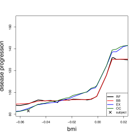
(a) Diabetes dataset.

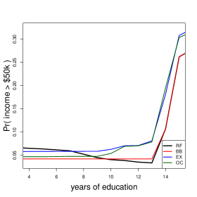
(b) Adult dataset.

Figure 4: Illustrating the result of reshaping. We choose a test point at random and make predictions with each model as we vary the predictor variable on the $x$-axis, holding all other variables constant. We see in both cases that the original RF predictions are not monotone-increasing. The Diabetes plot (4(a)) also shows the true value of the chosen data point with an X.

The solution to this optimization is of the form $\widetilde{\ell}_{i}=\mathop{\text{\rm min}}(c,\ell_{i})$ and $\widetilde{r}_{i}=\mathop{\text{\rm max}}(c,r_{i})$, for some constant $c$. Given the two sorted vectors $\ell$ and $r$, the optimization becomes:

$$\mathop{\text{\rm min}}_{c}\sum_{i=1}^{n_{1}}(\ell_{i}-\mathop{\text{\rm min}}(c,\ell_{i}))^{2}+\sum_{i=1}^{n_{2}}(r_{i}-\mathop{\text{\rm max}}(c,r_{i}))^{2}$$

This objective is convex and differentiable in $c$. Similar to the black box reshaping method, we can compute the derivatives at the values of the data and find where it flips sign, then compute the minimizer in the corresponding segment. This takes $O(n)$ time where $n=n_{1}+n_{2}$, the number of leaves under the shape-constrained split. With sorting, the over-constrained estimator can be computed in $O(n\log n)$ time for each shape-constrained split node.

We apply this procedure sequentially on the leaves of every shape-constrained node in reverse level-order on the tree.

3 Experiments

Table 1: Acronyms used for reshaping methods.

Method	Acronym	Sec
Random Forest	RF	-
Black Box Reshaping	BB	2.1
Exact Estimator	EX	2.2.1
Over-constrained Estimator	OC	2.2.2

We apply the reshaping methods described above to two regression tasks and two binary classification tasks. We show that reshaping allows us to enforce shape constraints without compromising predictive accuracy. For convenience, we use the acronyms in Table (1) to refer to each method.

The BB method was implemented in R, and the OC and EX methods were implemented in R and C++, extending the R package ranger (Wright & Ziegler, 2017). The exact estimator from Section (2.2.1) is computed using the MOSEK C++ package (ApS, 2017).

For binary classification, we use the probability tree implementation found in ranger, enforcing monotonicity of the probability of a positive classification with respect to the chosen predictors. For the purposes of these experiments, black box reshaping is applied to a traditional random forest. The random forest was fit with the default settings found in ranger.

We apply 5-fold cross validation on all four tasks and present the results under the relevant performance metrics in Table (2).

3.1 Diabetes Dataset

Table 2: Experimental results of 5-fold cross-validation. Accuracy is measured by mean squared error (Diabetes), mean absolute percent error (Zillow), and classification accuracy (Adult, Spam). Standard errors are shows in parentheses.

Method	Diabetes	Zillow	Adult	Spam
RF	3209 (377)	2.594% (0.1%)	87.0% (1.7%)	95.4% (1.3%)
BB	3210 (390)	2.594% (0.1%)	87.1% (1.8%)	95.4% (1.3%)
EX	3154 (353)	-	86.8% (1.5%)	95.3% (1.2%)
OC	3155 (350)	2.588% (0.1%)	87.0% (1.5%)	95.3% (1.2%)

The diabetes dataset (Efron et al., 2004) consists of ten physiological baseline variables, age, sex, body mass index, average blood pressure, and six blood serum measurements, for each of 442 patients. The response is a quantitative measure of disease progression measured one year after baseline.

Holding all other variables constant, we might expect disease progression to be monotonically increasing in body mass index (Ganz et al., 2014). We estimate a random forest and apply our reshaping techniques, then make predictions for a random test subject as we vary the body mass index predictor variable. The results shown in Figure (4(a)) illustrate the effect of reshaping on the predictions.

We use mean squared error to measure accuracy. The results in Table (2) indicate that the prediction accuracy of all four estimators is approximately the same.

3.2 Zillow Dataset

In this section, the regression task is to predict real estate sales prices using property information. The data were obtained from Zillow, an online real estate database company. For each of 206,820 properties, we are given the list price, number of bedrooms and bathrooms, square footage, build decade, sale year, major renovation year (if any), city, and metropolitan area. The response is the actual sale price of the home.

We reshape to enforce monotonicity of the sale price with respect to the list price. Due to the size of the constraint set, this problem becomes intractable for MOSEK; the results for the EX method are omitted. An interesting direction for future work is to investigate more efficient algorithms for this method.

Following reported results from Zillow, we use mean absolute percent error (MAPE) as our measure of accuracy. For an estimate $\widehat{y}$ of the true value $y$, the APE is $|\widehat{y}-y|/y$.

The results in Table (2) show that the performance across all estimators is indistinguishable.

3.3 Adult Dataset

We apply the reshaping techniques to the binary classification task found in the Adult dataset Lichman (2013). The task is to predict whether an individual’s income is less than or greater than $50,000. Following the experiments performed in Milani Fard et al. (2016) and You et al. (2017), we apply monotonic reshaping to four variables: capital gain, weekly hours of work, education level, and the gender wage gap.

We illustrate the effect of reshaping on the predictions in Figure (4(b)). The results in Table (2) show that we achieve similar test set accuracy before and after reshaping the random forest.

3.4 Spambase Dataset

Finally, we apply reshaping to classify whether an email is spam or not. The Spambase dataset (Lichman, 2013) contains 4,601 emails each with 57 predictors. There are 48 word frequency predictors, 6 character frequency predictors, and 3 predictors related to the number of capital letters appearing in the email.

That data were collected by Hewlett-Packard labs and donated by George Forman. One of the predictors is the frequency of the word “george”, typically assumed to be an indicator of non-spam for this dataset. We reshape the predictions to enforce the probability of being classified as spam to be monotonically decreasing in the frequency of words “george” and “hp”.

The results in Table (2) again show similar performance across all methods.

4 Discussion

We presented two strategies for prediction rule reshaping. We developed efficient algorithms to compute the reshaped estimators, and illustrated their properties on four datasets. Both approaches can be viewed as frameworks for developing more sophisticated reshaping techniques.

There are several ways that this work can be extended. Extensions to the black box method include adaptively combining rearrangements and isotonization (Chernozhukov et al., 2009), and considering a weighted objective function to account for the distance between test points.

In general, the random forest reshaping method can be viewed as operating on pre-trained parameters of a specific model. Applying this line of thinking to gradient boosted trees, deep learning methods, and other machine learning techniques could yield useful variants of this approach.

And finally, while practitioners might require certain shape-constraints on their predictions, many scientific applications also require inferential quantities, such as confidence intervals and confidence bands. Developing inferential procedures for reshaped predictions, similar to Chernozhukov et al. (2010) for rearrangements and Athey et al. (2018) for random forests, would yield interpretable predictions along with useful measures of uncertainty.

5 Acknowledgments

Research supported in part by ONR grant N00014-12-1-0762, NSF grants DMS-1513594 and DMS-1654076, and an Alfred P. Sloan fellowship.

References

- Amos et al. (2017) Amos, Brandon, Xu, Lei, and Kolter, J. Zico. Input convex neural networks. In Proceedings of the 34th International Conference on Machine Learning, 2017.
- ApS (2017) ApS, MOSEK. MOSEK Fusion API for C++ 8.0.0.94, 2017. URL https://docs.mosek.com/8.0/cxxfusion/index.html.
- Athey et al. (2018) Athey, S., Tibshirani, J., and Wager, S. Generalized Random Forests. Forthcoming in Annals of Statistics, 2018. URL https://arxiv.org/abs/1610.01271.
- Ayer et al. (1955) Ayer, Miriam, Brunk, H.D., Ewing, G.M., Reid, W.T., and Silverman, Edward. An empirical distribution function for sampling with incomplete information. Annals of Mathematical Statistics, 26:641–648, 1955.
- Ben-David (1995) Ben-David, Arie. Monotonicity maintenance in information-theoretic machine learning algorithms. Mach. Learn., 19(1):29–43, April 1995. ISSN 0885-6125. 10.1023/A:1022655006810.
- Breiman (2001) Breiman, Leo. Random forests. Mach. Learn., 45(1):5–32, October 2001. ISSN 0885-6125. 10.1023/A:1010933404324.
- Chen & Samworth (2016) Chen, Yining and Samworth, Richard J. Generalized additive and index models with shape constraints. Journal of the Royal Statistical Society: Series B (Statistical Methodology), 78(4):729–754, 2016.
- Chernozhukov et al. (2009) Chernozhukov, V., Fernández-Val, I., and Galichon, A. Improving point and interval estimators of monotone functions by rearrangement. Biometrika, 96(3):559–575, 2009.
- Chernozhukov et al. (2010) Chernozhukov, V., Fernández-Val, I., and Galichon, A. Quantile and probability curves without crossing. Econometrica, 78(3):1093–1125, 2010. ISSN 1468-0262.
- Efron et al. (2004) Efron, Bradley, Hastie, Trevor, Johnstone, Iain, and Tibshirani, Robert. Least angle regression. Annals of Statistics, 32:407–499, 2004.
- Feelders & Pardoel (2003) Feelders, Ad and Pardoel, Martijn. Pruning for monotone classification trees. In R. Berthold, Michael, Lenz, Hans-Joachim, Bradley, Elizabeth, Kruse, Rudolf, and Borgelt, Christian (eds.), Advances in Intelligent Data Analysis V, pp. 1–12, Berlin, Heidelberg, 2003. Springer Berlin Heidelberg.
- Ganz et al. (2014) Ganz, Michael L., Wintfeld, Neil, Li, Qian, Alas, Veronica, Langer, Jakob, and Hammer, Mette. The association of body mass index with the risk of type 2 diabetes: a case–control study nested in an electronic health records system in the united states. Diabetology & Metabolic Syndrome, 6(1):50, Apr 2014. ISSN 1758-5996.
- González et al. (2015) González, Sergio, Herrera, Francisco, and García, Salvador. Monotonic random forest with an ensemble pruning mechanism based on the degree of monotonicity. 33:367–388, 07 2015.
- Gupta et al. (2016) Gupta, Maya, Cotter, Andrew, Pfeifer, Jan, Voevodski, Konstantin, Canini, Kevin, Mangylov, Alexander, Moczydlowski, Wojciech, and van Esbroeck, Alexander. Monotonic calibrated interpolated look-up tables. Journal of Machine Learning Research, 17(109):1–47, 2016.
- Han & Wellner (2016) Han, Qiyang and Wellner, Jon A. Multivariate convex regression: global risk bounds and adaptation. arXiv preprint arXiv:1601.06844, 2016.
- Han et al. (2017) Han, Qiyang, Wang, Tengyao, Chatterjee, Sabyasachi, and Samworth, Richard J. Isotonic regression in general dimensions. arXiv preprint arXiv:1708.09468, 2017.
- Kyng et al. (2015) Kyng, Rasmus, Rao, Anup, and Sachdeva, Sushant. Fast, provable algorithms for isotonic regression in all l_p-norms. In Cortes, C., Lawrence, N. D., Lee, D. D., Sugiyama, M., and Garnett, R. (eds.), Advances in Neural Information Processing Systems 28, pp. 2719–2727. Curran Associates, Inc., 2015.
- Lichman (2013) Lichman, M. UCI machine learning repository, 2013. URL http://archive.ics.uci.edu/ml.
- Makino et al. (1996) Makino, Kazuhisa, Suda, Takashi, Yano, Kojin, and Ibaraki, Toshihide. Data analysis by positive decision trees. In CODAS, pp. 257–264, 1996.
- Malley et al. (2012) Malley, James D, Kruppa, Jochen, Dasgupta, Abhijit, Malley, Karen G, and Ziegler, Andreas. Probability machines: consistent probability estimation using nonparametric learning machines. Methods of Information in Medicine, 51(1):74, 2012.
- Milani Fard et al. (2016) Milani Fard, Mahdi, Canini, Kevin, Cotter, Andrew, Pfeifer, Jan, and Gupta, Maya. Fast and flexible monotonic functions with ensembles of lattices. In Lee, D. D., Sugiyama, M., Luxburg, U. V., Guyon, I., and Garnett, R. (eds.), Advances in Neural Information Processing Systems 29, pp. 2919–2927. Curran Associates, Inc., 2016.
- Potharst & Feelders (2002) Potharst, R. and Feelders, A. J. Classification trees for problems with monotonicity constraints. SIGKDD Explor. Newsl., 4(1):1–10, June 2002. ISSN 1931-0145.
- Pya & Wood (2015) Pya, Natalya and Wood, Simon N. Shape constrained additive models. Statistics and Computing, 25(3):543–559, May 2015. ISSN 1573-1375.
- Spouge et al. (2003) Spouge, J., Wan, H., and Wilbur, W.J. Least squares isotonic regression in two dimensions. Journal of Optimization Theory and Applications, 117(3):585–605, Jun 2003.
- Wright & Ziegler (2017) Wright, Marvin N. and Ziegler, Andreas. ranger: A fast implementation of random forests for high dimensional data in C++ and R. Journal of Statistical Software, 77(1):1–17, 2017.
- Xu et al. (2016) Xu, Min, Chen, Minhua, and Lafferty, John. Faithful variable screening for high-dimensional convex regression. Ann. Statist., 44(6):2624–2660, 12 2016. 10.1214/15-AOS1425.
- You et al. (2017) You, Seungil, Ding, David, Canini, Kevin, Pfeifer, Jan, and Gupta, Maya. Deep lattice networks and partial monotonic functions. In NIPS, 2017.