Task Agnostic Robust Learning on Corrupt Outputs
by Correlation-Guided Mixture Density Networks

Abstract

In this paper, we focus on weakly supervised learning with noisy training data for both classification and regression problems. We assume that the training outputs are collected from a mixture of a target and correlated noise distributions. Our proposed method simultaneously estimates the target distribution and the quality of each data which is defined as the correlation between the target and data generating distributions. The cornerstone of the proposed method is a Cholesky Block that enables modeling dependencies among mixture distributions in a differentiable manner where we maintain the distribution over the network weights. We first provide illustrative examples in both regression and classification tasks to show the effectiveness of the proposed method. Then, the proposed method is extensively evaluated in a number of experiments where we show that it constantly shows comparable or superior performances compared to existing baseline methods in the handling of noisy data.

1 Introduction

Training a deep neural network requires immense amounts of training data which are often collected using crowd-sourcing methods, such as Amazon’s Mechanical Turk (AMT). However, in practice, the crowd-sourced labels are often noisy [1]. Furthermore, naive training of deep neural networks is often vulnerable to over-fitting given the noisy training data in that they are capable of memorizing the entire dataset even with inconsistent labels, leading to a poor generalization performance [2]. We address this problem through the principled idea of revealing the correlations between the target distribution and the other (possibly noise) distributions by assuming that a training dataset is sampled from a mixture of a target distribution and other correlated distributions.

Throughout this paper, we aim to address the following two questions: 1) How can we define (or measure) the quality of training data in a principled manner? 2) In the presence of inconsistent outputs, how can we infer the target distribution in a scalable manner? Traditionally, noisy outputs are handled by modeling additive random distributions, often leading to robust loss functions [3] or estimating the structures of label corruptions in classifications tasks [4] (for more details, refer to Section 2).

To address the first question, we leverage the concept of a correlation. Precisely, we define and measure the quality of training data using the correlation between the target distribution and the data generating distribution. However, estimating the correct correlation requires access to the target distribution, whereas learning the correct target distribution requires knowing the correlation between the distributions to be known, making it a chicken-and-egg problem. To address the second question, we present a novel method that simultaneously estimates the target distribution as well as the correlation in a fully differentiable manner using stochastic gradient descent methods.

The cornerstone of the proposed method is a Cholesky Block in which we employ the Cholesky transform for sampling the weights of a neural network that enables us to model correlated outputs. Similar to Bayesian neural networks [5], we maintain the probability distributions over the weights, but we also leverage mixture distributions to handle the inconsistencies in a dataset. To the best of our knowledge, this is the first approach simultaneously to infer the target distribution and the output correlations using a neural network in an end-to-end manner. We will refer to this framework as ChoiceNet.

ChoiceNet is first applied to synthetic regression tasks and a real-world regression task where we demonstrate its robustness to extreme outliers and its ability to distinguish the target distribution and noise distributions. Subsequently, we move on to image classification tasks using a number of benchmark datasets where we show that it shows comparable or superior performances compared to existing baseline methods in terms of robustness with regard to handling different types of noisy labels.

2 Related Work

Recently, robustness in deep learning has been actively studied [6] as deep neural networks are being applied to diverse tasks involving real-world applications such as autonomous driving [7] or medical diagnosis [8] where a simple malfunction can have catastrophic results [9].

Existing work for handing noisy training data can be categorized into four groups: small-loss tricks [10, 11, 12, 13], estimating label corruptions [14, 15, 16, 17, 18, 19], using robust loss functions [20, 21], and explicit and implicit regularization methods [22, 23, 24, 25, 26, 27, 28, 29, 30]. Our proposed method is mostly related to the robust loss function approach but cannot fully be categorized into this group in that we present a novel architecture, a mixture of correlated densities network block, for achieving robustness based on the correlation estimation.

First of all, the small-loss tricks selectively focus on training instances based on a certain criterion, such as having small cost values [12]. [13] proposed a meta-algorithm for tackling the noisy label problem by training two networks only when the predictions of the two networks disagree, where selecting a proper network from among the two networks can be done using an additional clean dataset. [11] reweighs the weight of each training instance using a small amount of clean validation data. MentorNet [10] concentrated on the training of an additional neural network, which assigns a weight to each instance of training data to supervise the training of a base network, termed StudentNet, to overcome the over-fitting of corrupt training data. Recent work [12] presented Co-teaching by maintaining two separate networks where each network is trained with small-loss instances selected from its peer network.

The second group of estimating label corruption information is mainly presented for classification tasks where training labels are assumed to be corrupt with a possibly unknown corruption matrix. An earlier study in [17] proposed an extra layer for the modeling of output noises. [4] extended the approach mentioned above by adding an additional noise adaptation layer with aggressive dropout regularization. A similar method was then proposed in [14] which initially estimated the label corruption matrix with a learned classifier and used the corruption matrix to fine-tune the classifier. Other researchers [15] presented a robust training method that mimics the EM algorithm to train a neural network, with the label noise modeled as an additional softmax layer, similar to earlier work [4]. A self-error-correcting network was also presented [31]. It switches the training labels based on the learned model at the beginning stages by assuming that the deep model is more accurate during the earlier stage of training.

Researchers have also focussed on using robust loss functions; [20] studied the problem of binary classification in the presence of random labels and presented a robust surrogate loss function for handling noisy labels. Existing loss functions for classification were studied [32], with the results showing that the mean absolute value of error is inherently robust to label noise. In other work [21], a robust loss function for deep regression tasks was proposed using Tukey’s biweight function with the median absolute deviation of the residuals.

The last group focusses on using implicit or explicit regularization methods while training. Adding small label noises while training is known to be beneficial to training, as it can be regarded as an effective regularization method [23, 24]. Similar methods have been proposed to tackle noisy outputs. A bootstrapping method [22] which trains a neural network with a convex combination of the output of the current network and the noisy target was proposed. [25] proposed DisturbLabel, a simple method that randomly replaces a percentage of the labels with incorrect values for each iteration. Mixing both input and output data was also proposed [26, 27]. One study [27] considered the image recognition problem under label noise and the other [26] focused on a sound recognition problem. The temporal ensemble was proposed in [30] where an unsupervised loss term of fitting the output of an augmented input to the augmented target updated with an exponential moving average. [29] extends the temporal ensemble in [30] by introducing a consistency cost function that minimizes the distance between the weights of the student model and the teacher model. [28] presented a new regularization method based on virtual adversarial loss which measures the smoothness of conditional label distribution given input. Minimizing the virtual adversarial loss has a regularizing effect in that it makes the model smooth at each data point.

The foundation of the proposed method is a Cholesky Block where the output distribution is modeled using a mixture of correlated distributions. Modeling correlations of output training data has been actively studied in light of Gaussian processes [33]. MTGPP [34] that models the correlations of multiple tasks via Gaussian process regression was proposed in the context of a multi-task setting. [35] proposed a robust learning from demonstration method using a sparse constrained leverage optimization method which estimates the correlation between the training outputs and showed its robustness compared to several baselines.

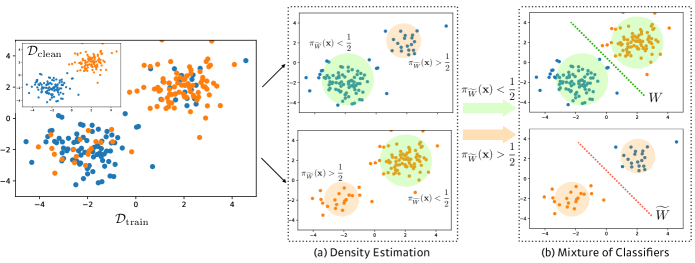
Figure 1: A process of binary classification on corrupt data using the mixture of (a) densities and (b) classifiers through (4). $\pi_{\widetilde{W}}(\mathbf{x})$ is the mixture weight which models the choice probability of $\widetilde{W}$ and estimates the corruption probability $\pi_{\text{corrupt}}$ in (3).

3 Proposed Method

In this section, we present the motivation and the model architecture of the proposed method. The main ingredient is a Cholesky Block which can be built on top of any arbitrary base network. First, we illustrate the motivations of designing the Cholesky Block in Section 3.1. Section 3.2 introduces a Cholesky transform which enables correlated sampling procedures. Subsequently, we present the overall mechanism of the proposed method and its loss functions for regression and classification tasks in Section 3.3 followed by illustrative synthetic examples in Section 3.4.

3.1 Motivation

Denote training data with correct (clean) labels by $\mathcal{D}_{\text{clean}}$ whose elements $(\mathbf{x},y)\in\mathcal{D}_{\text{clean}}$ are determined by a relation $y=f(\mathbf{x})$ for a regression task and $y\in L$ for a classification task where $L$ is a discrete set. In this paper, we assume that the corrupt training data $(\mathbf{x},\hat{y})\in\mathcal{D}_{\text{train}}$ is generated by

Regression:

$$\hat{y}=\begin{cases}f(\mathbf{x})+\epsilon&\text{with }1-p\\ g(\mathbf{x})+\xi&\text{with }p\end{cases}$$ (1)

Classification:

$$\hat{y}=\begin{cases}y&\text{with }1-p\\ L\setminus\{y\}&\text{with }p\end{cases}$$ (2)

where $g$ is an arbitrary function. Here $\epsilon$ and $\xi$ are heteroscedastic additive noises and $p$ indicates the corruption probability. Then, the above settings naturally employ the mixture of the conditional distributions:

$$P(\hat{y}|\mathbf{x})=(1-\pi_{\text{corrupt}})P_{\text{target}}(\hat{y}|\mathbf{x})+\pi_{\text{corrupt}}P_{\text{noise}}(\hat{y}|\mathbf{x})$$ (3)

where $\pi_{\text{corrupt}}$ models the corrupt ratio $p$. In particular, we model the target conditional density $P_{\text{target}}(\cdot|\cdot)$ using a parametrized distribution with a Gaussian distribution with a fixed variance $\hat{\sigma}^{2}$, i.e., $P(\cdot|\mathbf{x})=\mathcal{N}(f_{\mathbf{\theta}}(\mathbf{x}),\,\hat{\sigma}^{2})$ where $f_{\theta}(\cdot)$ can be any functions, e.g., a feed-forward network, parametrized with $\theta$.

While it may look similar to a Huber’s $\epsilon$-contamination model [36], one major difference is that, our method quantifies the irrelevance (or independence) of noise distributions by utilizing the input-dependent correlation $\rho(\mathbf{x})$ between $P_{\text{target}}(\cdot|\mathbf{x})$ and $P_{\text{noise}}(\cdot|\mathbf{x})$. To be specific, $P_{\text{noise}}(\cdot|\mathbf{x})$ will be a function of $P_{\text{target}}(\cdot|\mathbf{x})$ and $\rho(\mathbf{x})$.

In the training phase, we jointly optimize $P_{\text{target}}(\cdot|\mathbf{x})$ and $\rho(\mathbf{x})$. Intuitively speaking, irrelevant noisy data will be modeled to be collected from a class of $P_{\text{noise}}$ with relatively small or negative $\rho$ which can be shown in Figure 4. Since we assume that the correlation (quality) is not explicitly given, we model the $\rho$ of each data to be a function of an input $\mathbf{x}$ i.e., $\rho_{\phi}(\mathbf{x})$, parametrized by $\phi$ and jointly optimize $\phi$ and $\theta$.

Why correlation matters in mixture modeling?

Let us suppose a binary classification problem $L=\{-1,1\}$ and a feature map $h:\mathcal{X}\to\mathcal{F}$ and a (stochastic) linear functional $W:\mathcal{F}\to\mathbb{R}$ are given. For $(\mathbf{x},y)\in\mathcal{D}_{\text{clean}}$, we expect that $W$ and $h$ will be optimized as follows:

$$Wh(\mathbf{x})\sim\begin{cases}\mathcal{N}(\mu_{+},\sigma^{2})&:y=1\\ \mathcal{N}(\mu_{-},\sigma^{2})&:y=-1\end{cases},\quad\mu_{+}>0,\mu_{-}<0$$

so that $-Wh(\mathbf{x)}\cdot y<0$ holds. However, if corrupt training data are given by (2), the linear functional $W$ and the feature map $h(\cdot)$ may have $-Wh(\mathbf{x)}\cdot\hat{y}>0$ and using an ordinary loss function, such as a cross-entropy loss, might lead to over-fitting of the contaminated pattern of $\mathcal{D}_{\text{train}}$. Motivated from (3), we employ the mixture density to discriminate the corrupt data by using another linear classifier $\widetilde{W}$ which is expected to reveal the reverse patterns by minimizing the following mixture classification loss:

$$-\left\{(1-\pi_{\widetilde{W}}(\mathbf{x}))Wh(\mathbf{x})-\pi_{\widetilde{W}}(\mathbf{x})\widetilde{W}h(\mathbf{x})\right\}\cdot\hat{y}$$ (4)

Here $\pi_{\widetilde{W}}(\mathbf{x})$ is the mixture weight which models the choice probability of the reverse classifier $\widetilde{W}$ and eventually estimates the corruption probability $\pi_{\text{corrupt}}$ in (3). See Figure 1 for the illustrative example in binary classification.

However, the above setting is not likely to work in practice as both $W$ and $\widetilde{W}$ may learn the corrupt patterns independently hence $\pi_{\widetilde{W}}(\mathbf{x})$ adhere to $1/2$ under (4). In other words, the lack of dependencies between $W$ and $\widetilde{W}$ makes it hard to distinguish clean and corrupt patterns. To aid $W$ to learn the pattern of data with a clean label, we need a self-regularizing way to help $\pi_{\widetilde{W}}$ to infer the corruption probability of given data point $\mathbf{x}$ by guiding $\widetilde{W}$ to learn the reverse mapping of given feature $h(\mathbf{x})$. To resolve this problem, let us consider different linear functional $\widehat{W}$ with negative correlation with $W$, i.e., $\rho(\widehat{W},W)<0$. Then this functional maps the feature $h(\mathbf{x})$ as follows:

$$\widehat{W}h(\mathbf{x})\sim\begin{cases}\mathcal{N}(\rho\mu_{+},\sigma^{2})&:y=1\\ \mathcal{N}(\rho\mu_{-},\sigma^{2})&:y=-1\end{cases}$$

since $\rho(\widehat{W},W)=\rho(\widehat{W}h,Wh)$ so we have $-\widehat{W}h(\mathbf{x})\cdot\hat{y}<0$ if $\hat{y}=-y$. Eventually, (4) is minimized when $\pi_{\widehat{W}}(\mathbf{x})\approx 1$ if output is corrupted, i.e., $\hat{y}=-y$, and $\pi_{\widetilde{W}}(\mathbf{x})\approx 0$ otherwise. In this way, we can make $\pi_{\widehat{W}}(\mathbf{x})$ to learn the corrupt probability for given data point.

We provide illustrative examples in both regression and classification that can support the aforementioned motivation in Section 3.4.

3.2 Cholesky Block for Correlated Sampling

Now we introduce a Cholesky transform that enables modeling dependencies among output mixtures in a differentiable manner. The Cholesky transform is a way of constructing a random variable which is correlated with other random variables and can be used as a sampling routine for sampling correlated matrices from two uncorrelated random matrices.

To be specific, suppose that $w\sim\mathcal{N}(\mu_{w},\,\sigma^{2}_{w})$ and $z\sim\mathcal{N}(0,\,\sigma^{2}_{z})$ and our goal is to construct a random variable $\tilde{w}$ such that the correlation between $w$ and $\tilde{w}$ becomes $\rho$. Then, the Cholesky transform which is defined as

$$\text{{Cholesky}}(w,z,\rho,\mu_{w},\sigma_{w},\sigma_{z})$$ (5)

$$:=\rho\mu+\sqrt{1-\rho^{2}}\left(\rho\frac{\sigma_{z}}{\sigma_{w}}(w-\mu)+z\sqrt{1-\rho^{2}}\right)$$

is a mapping from $(w,z)\in\mathbb{R}^{2}$ to $\mathbb{R}$ and can be used to construct $\tilde{w}$. In fact, $\tilde{w}=\text{{Cholesky}}(w,z,\rho,\mu_{w},\sigma_{w},\sigma_{z})$ and we can easily use (5) to construct a feed-forward layer with a correlated weight matrix which will be referred to as a Cholesky Block as shown in Figure 2.

We also show that the correlation is preserved through the affine transformation making it applicable to a single fully-connected layer where all the derivations and proofs can be found in the supplementary material. In other words, we model correlated outputs by first sampling correlated weight matrices using Cholesky transfrom in an element-wise fashion and using the sampled weights for an affine transformation of a feature vector of a feed-forward layer. One can simply use a reparametrization trick [37] for implementations.

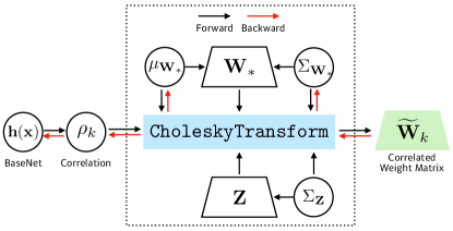
Figure 2: Illustration of a Cholesky Block. Every block shares target weight matrix $\mathbf{W}_{*}$ and auxiliary matrix $\mathbf{Z}$, and outputs correlated weight matrix $\widetilde{\mathbf{W}}_{k}$ through CholeskyTransform (see (5)) to distinguish the abnormal pattern from normal one which will be learned by $\mathbf{W}_{*}$.

3.3 Overall Mechanism of ChoiceNet

In this section we describe the model architecture and the overall mechanism of ChoiceNet. In the following, $\tau^{-1}>0$ is a small constant indicating the expected variance of the target distriubtion. $\mathbf{W}_{\mathbf{h}\to\boldsymbol{\rho}}$, $\mathbf{W}_{\mathbf{h}\to\boldsymbol{\pi}}\in\mathbb{R}^{K\times Q}$ and $\mathbf{W}_{\mathbf{h}\to\boldsymbol{\Sigma_{0}}}\in\mathbb{R}^{D\times Q}$ are weight matrices where $Q$ and $D$ denote the dimensions of a feature vector $\mathbf{h}$ and output $\mathbf{y}$, respectively, and $K$ is the number of mixtures.

ChoiceNet is a twofold architecture: (a) an arbitrary base network and (b) the Cholesky Block (see Figure 2). Once the base network extracts features, The Cholesky Block estimates the mixture of the target distribution and other correlated distributions using the Cholesky transform in (5). While it may seem to resemble a mixture density network (MDN) [38], this ability to model dependencies between mixtures lets us to effectively infer and distinguish the target distributions from other noisy distributions as will be shown in the experimental sections. When using the MDN, particularly, it is not straightforward to select which mixture to use other than using the one with the largest mixture probability which may lead to inferior performance given noisy datasets.

Let us elaborate on the overall mechanism of ChoiceNet. Given an input $\mathbf{x}$, a feature vector $\mathbf{h}\in\mathbb{R}^{Q}$ is computed from any arbitrary mapping such as ResNet [39] for images or word embedding [40] for natural languages. Then the network computes $K-1$ correlations, $\{\rho_{1},\rho_{2}(\mathbf{h}),...,\rho_{K}(\mathbf{h})\}$, for $K$ mixtures where the first $\rho_{1}=1$ is reserved to model the target distribution, In other words, the first mixture becomes our target distribution and we use the predictions from the first mixture in the inference phase.

The mean and variance of the weight matrix, $\mu_{\mathbf{W}}\in\mathbb{R}^{Q\times D}$ and $\Sigma_{\mathbf{W}}\in\mathbb{R}^{Q\times D}$, are defined and updated for modeling correlated output distributions which is analogous to a Bayesian neural network [5], These matrices can be back-propagated using the reparametrization trick. The Cholesky Block also computes the base output variance $\Sigma_{0}(\mathbf{h})$ similar to an MDN.

Then we sample $K$ weight matrices $\{\widetilde{\mathbf{W}}_{i}\}_{i=1}^{K}$ from $\{\mu_{*},\Sigma_{*}\}$ and $\{\rho_{1},\rho_{2}(\mathbf{h}),...,\rho_{K}(\mathbf{h})\}$ using the Cholesky transform (5) so that the correlations between $\widetilde{\mathbf{W}}_{i}$ and $\mathbf{W}_{*}$ becomes $\rho_{i}(\cdot)$. Note that the correlation is preserved through an affine transform. The $K$ sampled feedforward weights, $\{\widetilde{\mathbf{W}}_{i}\}_{i=1}^{K}$, are used to compute $K$ correlated output mean vectors, $\{\mu_{i}\}_{i=1}^{K}$. Note that the correlation between $\mu_{1}$ and $\mu_{i}$ also becomes $\rho_{i}(\cdot)$. We would like to emphasize that, as we employ Gaussian distributions in the Cholesky transform, the influences of uninformative or independent data, whose correlations, $\rho$, are close to $0$, is attenuated as their variances increase [41].

Input : $\mathcal{D}_{\text{train}}$, $K$, $\tau$, $\lambda$, $\mathbf{h}:\mathcal{X}\to\mathbb{R}^{Q}$

Initialize $\mu_{*},\Sigma_{*},\Sigma_{\mathbf{Z}}\in\mathbb{R}^{Q\times D}$

$\qquad\qquad\mathbf{W}_{\mathbf{h}\to\boldsymbol{\rho}},\mathbf{W}_{\mathbf{h}\to\boldsymbol{\pi}},\mathbf{W}_{\mathbf{h}\to\Sigma_{0}}\in\mathbb{R}^{K\times Q}$

while True do

       Sample $\mathbf{W}_{*}\sim\mathcal{N}(\mu_{*},\Sigma_{*})$, $\mathbf{Z}\sim\mathcal{N}(\boldsymbol{0},\Sigma_{\mathbf{Z}})$

      for $k\in\{1,\ldots,K\}$ do

             $\rho_{k}=\tanh(\mathbf{W}_{\mathbf{h}\to\boldsymbol{\rho}}\mathbf{h})_{k}$ $\qquad(\rho_{1}=1)$

             $\pi_{k}=\text{softmax}(\mathbf{W}_{\mathbf{h}\to\boldsymbol{\pi}}\mathbf{h})_{k}$

             $(\Sigma_{0})_{k}=\exp(\mathbf{W}_{\mathbf{h}\to\Sigma_{0}}\mathbf{h})_{k}$

             $\Sigma_{k}=(1-\rho_{k}^{2})(\Sigma_{0})_{k}+\tau^{-1}$

             $\widetilde{\mathbf{W}}_{k}$ = Cholesky$(\mathbf{W}_{*},\mathbf{Z},\rho_{k},\mu_{*},\Sigma_{*},\Sigma_{\mathbf{Z}})$

             $\mu_{k}=\widetilde{\mathbf{W}}_{k}\mathbf{h}$

       end for

      

      Compute $\mathcal{L}(\mathcal{D}_{\text{train}}|(\pi_{k},\mu_{k},\Sigma_{k})_{k=1}^{K})$

      

      Update $\mathbf{h},\mathbf{W}_{\mathbf{h}\to\boldsymbol{\rho}},\mathbf{W}_{\mathbf{h}\to\boldsymbol{\pi}},\mathbf{W}_{\mathbf{h}\to\Sigma_{0}},\mu_{*},\Sigma_{*}$

end while

return $\mathbf{W}_{*},\mathbf{h}$

Algorithm 1 ChoiceNet Algorithm

The output variances of $k$-th mixture is computed from $\rho_{k}(\mathbf{h})$ and the based output variance $\Sigma_{0}(\mathbf{h})$ as follows:

$$\Sigma_{k}=(1-\rho^{2}_{k}(\mathbf{h}))\Sigma_{0}(\mathbf{h})+\tau^{-1}\in\mathbb{R}^{D}$$ (6)

This has an effect of increasing the variance of the mixture which is less related (in terms of the absolute value of a correlation) with the target distribution. The Cholesky Block also computes the mixture probabilities of $k$-th mixture, $\pi_{k}(\mathbf{h})$, akin to an MDN. The overall process of the Cholesky Block is summarized in Algorithm 1 and Figure 3. Now, let us introduce the loss functions for regression and classification tasks.

Regression

For the regression task, we employ both $L_{2}$-loss and the standard MDN loss ([38, 42, 43])

$$\mathcal{L}(\mathcal{D})=\frac{1}{N}\sum_{i=1}^{N}\lambda_{1}\|\mathbf{y}_{i}-\mu_{1}(\mathbf{x}_{i})\|_{2}^{2}$$ (7)

$$+\frac{1}{N}\sum_{i=1}^{N}\lambda_{2}\log\left(\sum_{k=1}^{K}\pi_{k}(\mathbf{x}_{i})\mathcal{N}(\mathbf{y}_{i};\mu_{k}(\mathbf{x}_{i}),\Sigma_{k}(\mathbf{x}_{i}))\right)$$

where $\lambda_{1}$ and $\lambda_{2}$ are hyper-parameters and $\mathcal{N}(\cdot|\mu,\Sigma)$ is the density of multivariate Gaussian:

$$\mathcal{N}(\mathbf{y}_{i};\mu_{k},\Sigma_{k})=\prod_{d=1}^{D}\frac{1}{\sqrt{2\pi\Sigma_{k}^{(d)}}}\exp\left(-\frac{|y_{i}^{(d)}-\mu_{k}^{(d)}|^{2}}{2\Sigma_{k}^{(d)}}\right)$$

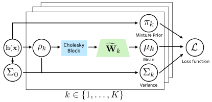
Figure 3: Overall mechanism of ChoiceNet. It consists of $K$ mixtures and each mixture outputs triplet $(\pi_{k},\mu_{k},\Sigma_{k})$ via Algorithm 1. $\rho_{1}=1$ is reserved to model the target distribution.

We also propose the following Kullback-Leibler regularizer:

$$\mathbb{KL}(\bar{\boldsymbol{\rho}}\|\boldsymbol{\pi})=\sum_{k=1}^{K}\bar{\boldsymbol{\rho}}_{k}\log\frac{\bar{\boldsymbol{\rho}}_{k}}{\pi_{k}},\quad\bar{\boldsymbol{\rho}}=\text{softmax}(\boldsymbol{\rho})$$ (8)

The above KL regularizer encourages the mixture components with the strong correlations to have high mixture probabilities. Note that we use the notion of correlation to evaluate the goodness of each training data where the first mixture whose correlation is always $1$ is reserved for modeling the target distribution.

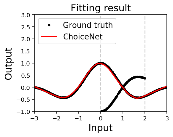
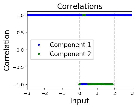
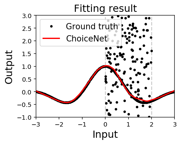
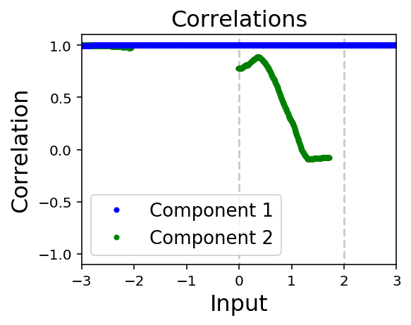
Figure 4: Fitting results on datasets with (a) flipped function and (c) uniform corruptions. Resulting correlations of two components with (b) flipped function and (d) uniform corruptions.

Classification

In the classification task, we suppose each $\mathbf{y}_{i}$ is a $D$-dimensional one-hot vector. Unlike the regression task, (LABEL:loss-reg) is not appropriate for the classification task. We employ the following loss function:

$$\mathcal{L}(\mathcal{D})=-\frac{1}{N}\sum_{i=1}^{N}\sum_{k=1}^{K}\pi_{k}(\mathbf{x}_{i})l(\mathbf{x}_{i},\mathbf{y}_{i})$$ (9)

where

$$l(\mathbf{x}_{i},\mathbf{y}_{i}) =\langle\text{softmax}(\hat{\mathbf{y}}_{k}(\mathbf{x}_{i})),\mathbf{y}_{i}\rangle$$

$$\qquad-\lambda_{\text{reg}}\log\left(\sum_{d=1}^{D}\exp(\hat{y}_{k}^{(d)}(\mathbf{x}_{i}))\right).$$

Here $\langle\cdot,\cdot\rangle$ denotes inner product, $\hat{\mathbf{y}}_{k}=(\hat{y}_{k}^{(1)},\ldots,\hat{y}_{k}^{(D)})$, and $\hat{y}_{k}^{(d)}(\mathbf{x}_{i})=\mu_{k}^{(d)}+\sqrt{\Sigma_{k}^{(d)}}\varepsilon$ where $\varepsilon\sim\mathcal{N}(0,1)$. Similar loss function was used in [44] which also utilizes a Gaussian mixture model.

3.4 Illustrative Synthetic Examples

Here, we provide synthetic examples in both regression and classification to illustrate how the proposed method can be used to robustly learn the underlying target distribution given a noisy training dataset.

Regression Task

We first focus on how the proposed method can distinguish between the target distribution and noise distributions in a regression task and show empirical evidence that our method can achieve this by estimating the target distribution and the correlation of noise distribution simultaneously. We train on two datasets with the same target function but with different types of corruptions by replacing $50\%$ of the output values whose input values are within $0$ to $2$: one uniformly sampled from $-1$ to $3$ and the other from a flipped target function as shown in Figure 4 and 4. Throughout this experiment, we set $K=2$ for better visualization.

As shown in Figure 4, ChoiceNet successfully estimates the target function with partial corruption. To further understand how ChoiceNet works, we also plot the correlation of each mixture at each input with different colors. When using the first dataset where we flip the outputs whose inputs are between $0$ and $2$, the correlations of the second mixture at the corrupt region becomes $-1$ (see Figure 4). This is exactly what we wanted ChoiceNet to behave in that having $-1$ correlation will simply flip the output. In other words, the second mixture takes care of the noisy (flipped) data by assigning $-1$ correlation while the first mixture component reserved for the target distribution is less affected by the noisy training data.

When using the second dataset, the correlations of the second mixture at the corrupt region are not $-1$ but decreases as the input increase from $0$ to $2$ (see Figure 4). Intuitively speaking, this is because the average deviations between the noisy output and the target output increases as the input increases. Since decreasing the correlation from $1$ to $0$ will increase the output variance as shown in (6), the correlation of the second mixture tends to decrease as the input increase between $0$ to $2$. This clearly shows the capability of ChoiceNet to distinguish the target distribution from noisy distributions.

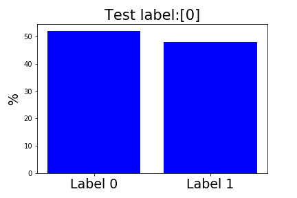
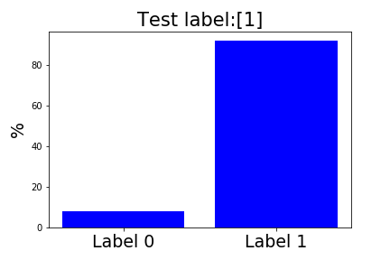
Figure 5: The predictions results of the second mixture of test inputs whose labels are (a) $0$ and (b) $1$, respectively.

Binary Classification Task

We also provide an illustrative binary classification task using label $0$ and $1$ from the MNIST dataset. In particular, we replaced $40\%$ of the training data with label $0$ to $1$. To implement ChoiceNet, we use two-layer convolutional neural networks with $64$ channels and two mixtures. We trained ChoiceNet for $10$ epochs where the final train and test accuracies are $81.7\%$ and $98.1\%$, respectively, which indicates ChoiceNet successfully infers clean data distribution. As the first mixture is deserved for inferring the clean target distribution, we expect the second mixture to take away corrupted labels. Figure 5 shows two prediction results of the second mixture when given test inputs with label $0$ and $1$. As $40\%$ of training labels whose labels are originally $0$ are replaced to $1$, almost half of the second mixture predictions of test images whose labels are $0$ are $1$ indicating that it takes away corrupted labels while training. On the contrary, the second mixture predictions of test inputs whose original labels are $1$ are mostly focusing on label $1$.

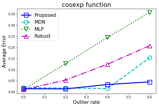
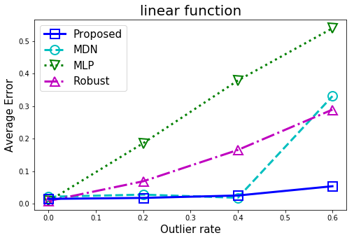
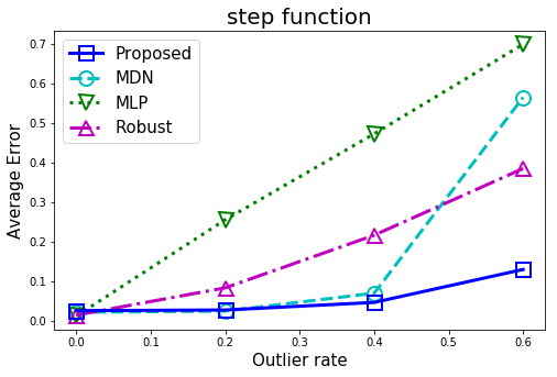
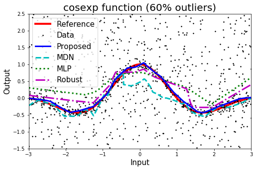
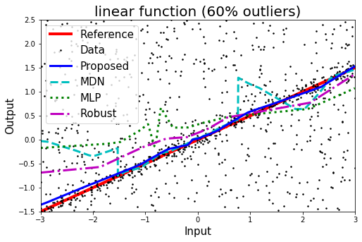
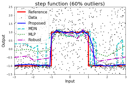
Figure 6: (a-c) Average fitting errors while varying the outlier rates and (e-f) fitting results of the compared methods with $60\%$ outliers using cosexp, linear, and step functions.

4 Experiments

In this section, we validate the performance of ChoiceNet on both regression problems in Section B.1 and classification problems in Section B.2 where we mainly focus on evaluating the robustness of the proposed method.

4.1 Regression Tasks

Here, we show the regression performances using synthetic regression tasks and a Boston housing dataset with outliers. More experimental results using synthetic data and behavior cloning scenarios in MuJoCo environments where the demonstrations are collected and mixed from both expert and adversarial policies as well as detailed experimental settings can be found in the supplementary material.

Synthetic Data

In order to evaluate the robustness of the proposed method, we use three different $1$-D target functions. Particularly, we use the following target functions: cosexp, linear, and step functions as shown in Figure 6-6, respectively, and collected $1,000$ points per each function while replacing a certain portion of outputs to random values uniformly sampled between $-1.5$ and $2.5$. We compared our proposed method with a mixture density network (MDN) [38] and fully connected layers with an $L_{2}$-loss (MLP) and a robust loss (Robust) proposed in [21]. We use three-layers with $64$ units and ReLU activations, and for both the proposed method and an MDN, five mixtures are used.

The average absolute fitting errors of three different functions are shown in Figure 6-6, respectively where we can see that the proposed method outperforms or show comparable results with low outlier rates and shows superior performances with a high outlier rate ($>50\%$). Figure 6-6 show the fitting results along with training data. While our proposed method is built on top of an MDN, it is worthwhile noting the severe performance degradation of an MDN with an extreme noise level ($60\%$). It is mainly because an MDN fails to allocate high mixture probability on the mixture corresponds to the target distribution as there are no dependencies among different mixtures.

Boston Housing Dataset

A Boston housing price dataset is used to check the robustness of the proposed method. We compare our method with standard feedforward networks using four different loss functions: standard $L2$-loss, $L1$-loss which is known to be robust to outliers, a robust loss (RL) function proposed in [21], and a leaky robust loss (LeakyRL) function where the results are shown in Table 5. Implementation details can be found in the supplementary material.

Table 1: The RMSEs of compared methods on the Boston Housing Dataset

Outliers	ChoiceNet	$L2$	$L1$	RL	LeakyRL	MDN
$0\%$	$3.29$	3.22	$3.26$	$4.28$	$3.36$	$3.46$
$10\%$	3.99	$5.97$	$5.72$	$6.36$	$5.71$	$6.5$
$20\%$	4.77	$7.51$	$7.16$	$8.08$	$7.08$	$8.62$
$30\%$	5.94	$9.04$	$8.65$	$10.54$	$8.67$	$8.97$
$40\%$	6.80	$9.88$	$9.69$	$10.94$	$9.68$	$10.44$

Table 2: Test accuracies on the CIFAR-10 dataset with by symmetric and asymmetric noises.

	Pair-$45\%$	Sym-$50\%$	Sym-$20\%$
Standard	49.5	48.87	76.25
+ ChoiceNet	70.3	85.2	91.0
MentorNet	58.14	71.10	80.76
Co-teaching	72.62	74.02	82.32
F-correction	6.61	59.83	59.83
MDN	51.4	58.6	81.4

		MNIST		FMNIST		SVHN		CIFAR10		CIFAR100
Data	Model	20%	50%	20%	50%	20%	50%	20%	50%	20%	50%
$D_{\text{test}}$	WideResNet	82.19	56.63	82.32	56.55	82.21	55.94	81.93	54.97	80.19	50.48
	+ ChoiceNet	99.66	99.03	97.46	95.36	94.40	78.32	96.58	90.28	85.81	68.89
$D_{\text{train}}$	WideResNet	99.29	92.49	98.62	92.42	99.34	95.91	99.97	99.82	99.96	99.91
	+ ChoiceNet	81.99	55.38	80.63	54.45	78.99	48.69	81.88	56.83	26.03	18.14
Expected True Ratio		82%	55%	82%	55%	82%	55%	82 %	55%	80.2%	50.5 %

Table 3: The comparison between naive WideResNet and ChoiceNet on multile benchmark datasets.

4.2 Classification Tasks

Here, we conduct comprehensive classification experiments to investigate how ChoiceNet performs on image classification tasks with noisy labels. More experimental results on MNIST, CIFAR-10, and a natural language processing task and ablation studies of hyper-parameters can also be found in the supplementary material.

CIFAR-10 Comparison

We first evaluate the performance of our method and compare it with MentorNet [10], Co-teaching [12] and F-correction [14] on noisy CIFAR-10 datasets. We follow three different noise settings from [12]: PairFlip-$45\%$, Symmetry-$50\%$, and Symmetry-$20\%$. On ‘Symmetry‘ settings, noisy labels can be assigned to all classes, while, on ‘PairFlip‘ settings, all noisy labels from the same true label are assigned to a single noisy label. A model is trained on a noisy dataset and evaluated on the clean test set. For fair comparisons, we keep other configurations such as the network topology to be the same as [12].

Table 14 shows the test accuracy of compared methods under different noise settings. Our proposed method outperforms all compared methods on the symmetric noise settings with a large margin over 10%p. On asymmetric noise settings (Pair-$45\%$), our method shows the second best performance, and this reveals the weakness of the proposed method. As Pair-$45\%$ assigns $45\%$ of each label to its next label, The Cholesky Block fails to infer the dominant label distributions correctly. However, we would like to note that Co-teaching [12] is complementary to our method where one can combine these two methods by using two ChoiceNets and update each network using Co-teaching.

Generalization to Other Datasets

We conduct additional experiments to investigate how our method works on other image datasets. We adopt the structure of WideResNet [45] and design a baseline network with a depth of $22$ and a widen factor of $4$. We also construct ChoiceNet by replacing the last two layers (‘average pooling‘ and ‘linear‘) with the Cholesky Block. We train the networks on CIFAR-10, CIFAR-100, FMNIST, MNIST and SVHN datasets with noisy labels. We generate noisy datasets with symmetric noise setting and vary corruption ratios from $20\%$ to $50\%$. We would like to emphasize that we use the same hyper-parameters, which are tuned for the CIFAR-10 experiments, for all the datasets except for CIFAR-100.

Table 3 shows test accuracies of our method and the baseline on various image datasets with noisy labels. ChoiceNet consistently outperforms the baseline in most of the configurations except for $80\%$-corrupted SVHN dataset. Moreover, we expect that performance gains can increase when dataset-specific hyperparameter tuning is applied. The results suggest that the proposed ChoiceNet can easily be applied to other noisy datasets and show a performance improvement without large efforts.

We would like to emphasize that the training accuracy of the proposed method in Table 3 is close to the expected true ratio. This implies that our proposed Cholesky Block can separate true labels and false labels from a noisy dataset. We also note that training ChoiceNet on CIFAR-100 datasets requires a modification in a loss weight. We hypothesize that the hyperparameters of our proposed method are sensitive to a number of target classes in a dataset.

5 Conclusion

In this paper, we have presented ChoiceNet that can robustly learn a target distribution given noisy training data. The keystone of ChoiceNet is the mixture of correlated densities network block which can simultaneously estimate the underlying target distribution and the quality of each data where the quality is defined by the correlation between the target and generating distributions. We have demonstrated that the proposed method can robustly infer the target distribution on corrupt training data in both regression and classification tasks. However, we have seen that in the case of extreme asymmetric noises, the proposed method showed suboptimal performances. We believe that it could resolved by combining our method with other robust learning methods where we have demonstrated that ChoiceNet can effectively be combined with mix-up [27]. Furthermore, one can use ChoiceNet for active learning by evaluating the quality of each training data using through the lens of correlations.

Appendix A Proof of Theorem in Section 3

In this appendix, we introduce fundamental theorems which lead to Cholesky transform for given random variables $(W,Z)$. We apply this transform to random matrices $\mathbf{W}$ and $\mathbf{Z}$ which carry out weight matrices for prediction and a supplementary role, respectively. We also elaborate the details of conducted experiments with additional illustrative figures and results. Particularly, we show additional classification experiments with the MNST dataset on different noise configurations.

Lemma 1.

Let $W$ and $Z$ be uncorrelated random variables such that

$$\begin{cases}\mathbb{E}W=\mu_{W},&\mathbb{V}\left(W\right)=\sigma_{W}^{2}\\ \mathbb{E}Z=0,&\mathbb{V}\left(Z\right)=\sigma_{Z}^{2}\end{cases}$$ (10)

For a given $-1\leq\rho\leq 1$, set

$$\tilde{Z}=\rho\frac{\sigma_{Z}}{\sigma_{W}}(W-\mu_{W})+\sqrt{1-\rho^{2}}Z$$ (11)

Then $\mathbb{E}\tilde{Z}=0$, $\mathbb{V}(\tilde{Z})=\sigma_{Z}^{2}$, and $\text{\rm{Corr}}(W,\tilde{Z})=\rho$.

Proof.

Since $W$ and $Z$ are uncorrelated, we have

$$\mathbb{E}\left[(W-\mu_{W})Z\right]=\mathbb{E}(W-\mu_{W})\mathbb{E}Z=0$$ (12)

By (10), we directly obtain

$$\mathbb{E}\tilde{Z}=\rho\frac{\sigma_{Z}}{\sigma_{W}}\left(\mathbb{E}W-\mu_{W}\right)+\mathbb{E}Z=0$$

Also, by (10) and (12),

$$\mathbb{V}\left(\tilde{Z}\right)=\mathbb{E}|\tilde{Z}|^{2} =\rho^{2}\left(\frac{\sigma_{Z}}{\sigma_{W}}\right)^{2}\mathbb{V}(W)+\mathbb{V}(Z)+2\rho\frac{\sigma_{Z}}{\sigma_{W}}\underbrace{\mathbb{E}\left[(W-\mu_{W})Z\right]}_{=0}$$

$$=\rho^{2}\frac{\sigma_{Z}^{2}}{\sigma_{W}^{2}}\sigma_{W}^{2}+(1-\rho^{2})\sigma_{Z}^{2}=\sigma_{Z}^{2}$$

Similarly,

$$\text{Cov}(W,\tilde{Z}) =\mathbb{E}\left[(W-\mu_{W})\tilde{Z}\right]$$

$$=\mathbb{E}\left[(W-\mu_{W})\rho\frac{\sigma_{Z}}{\sigma_{W}}(W-\mu_{W})\right]+\underbrace{\mathbb{E}\left[(W-\mu_{W})Z\right]}_{=0}$$

$$=\rho\frac{\sigma_{Z}}{\sigma_{W}}\mathbb{V}(W)=\rho\sigma_{Z}\sigma_{W}$$

Therefore

$$\text{Corr}(W,\tilde{Z})=\frac{\text{Cov}(W,\tilde{Z})}{\sqrt{\mathbb{V}(W)}\sqrt{\mathbb{V}(\tilde{Z})}}=\frac{\rho\sigma_{W}\sigma_{Z}}{\sigma_{W}\sigma_{Z}}=\rho$$

The lemma is proved. ∎

Lemma 2.

Assume the same condition in Lemma 1 and define $\tilde{Z}$ as (11). For given functions $\varphi:\mathbb{R}\to\mathbb{R}$ and $\psi:\mathbb{R}\to(0,\infty)$, set $\tilde{W}:=\varphi(\rho)+\psi(\rho)\tilde{Z}$. Then

$$\mathbb{E}\tilde{W}=\varphi(\rho),\quad\mathbb{V}(\tilde{W})=|\psi(\rho)|^{2}\sigma_{Z}^{2},\quad\text{\rm{Corr}}(W,\tilde{W})=\rho$$

Proof.

Note that

$$\mu_{\tilde{W}}=\varphi(\rho)+\psi(\rho)\mu_{\tilde{Z}}=\varphi(\rho)$$

$$\sigma_{\tilde{W}}^{2}=\left|\psi(\rho)\right|^{2}\mathbb{E}\left(\tilde{Z}-\mu_{\tilde{Z}}\right)^{2}=\psi^{2}(\rho)\sigma_{Z}^{2}$$

Therefore, by Lemma 1

$$\mathbb{E}\left[(W-\mu_{W})(\tilde{W}-\mu_{\tilde{W}})\right] =\psi(\rho)\mathbb{E}\left[(W-\mu_{W})(\tilde{Z}-\mu_{\tilde{Z}})\right]$$

$$=\rho\psi(\rho)\sigma_{W}\sigma_{Z}$$

Hence

$$\text{\rm{Corr}}(W,\tilde{W})=\frac{\mathbb{E}\left[(W-\mu_{W})(\tilde{W}-\mu_{\tilde{W}})\right]}{\sigma_{W}\sigma_{\tilde{W}}}=\frac{\rho\psi(\rho)\sigma_{W}\sigma_{Z}}{\psi(\rho)\sigma_{W}\sigma_{Z}}=\rho$$

The lemma is proved. ∎

Now we prove the aforementioned theorem in Section 3.

Theorem.

Let $\boldsymbol{\rho}=(\rho_{1},\ldots,\rho_{K})\in\mathbb{R}^{K}$. For $p\in\{1,2\}$, random matrices $\mathbf{W}^{(p)}\in\mathbb{R}^{K\times Q}$ are given such that for every $k\in\{1,\ldots,K\}$,

$$\text{\rm{Cov}}\left(W_{ki}^{(p)},W_{kj}^{(p)}\right)=\sigma_{p}^{2}\delta_{ij},\quad\text{\rm{Cov}}\left(W_{ki}^{(1)},W_{kj}^{(2)}\right)=\rho_{k}\sigma_{1}\sigma_{2}\delta_{ij}$$ (13)

Given $\mathbf{h}=(h_{1},\ldots,h_{Q})\in\mathbb{R}^{Q}$, set $\mathbf{y}^{(p)}=\mathbf{W}^{(p)}\mathbf{h}$ for each $p\in\{1,2\}$. Then an elementwise correlation between $\mathbf{y}^{(1)}$ and $\mathbf{y}^{(2)}$ equals $\boldsymbol{\rho}$ i.e.

$$\text{\rm{Corr}}\left(y_{k}^{(1)},y_{k}^{(2)}\right)=\rho_{k},\quad\forall k\in\{1,\ldots,K\}$$

Proof.

First we prove that for $p\in\{1,2\}$ and $k\in\{1,\ldots,K\}$

$$\mathbb{V}\left(y_{k}^{(p)}\right)=\sigma_{p}^{2}\left\|\mathbf{h}\right\|^{2}$$ (14)

Note that

$$\mathbb{V}\left(y_{k}^{(p)}\right) =\mathbb{E}\left[\left(\sum_{i=1}^{Q}W_{ki}^{(p)}h_{i}-\mathbb{E}\left[\sum_{i=1}^{Q}W_{ki}^{(p)}h_{i}\right]\right)^{2}\right]$$

$$=\mathbb{E}\left[\left(\sum_{i=1}^{Q}\left(W_{ki}^{(p)}-\mathbb{E}W_{ki}^{(p)}\right)h_{i}\right)^{2}\right]$$

$$=\mathbb{E}\left[\sum_{i,j}^{Q}\left(W_{ki}^{(p)}-\mathbb{E}W_{ki}^{(p)}\right)\left(W_{kj}^{(p)}-\mathbb{E}W_{kj}^{(p)}\right)h_{i}h_{j}\right]$$

$$=\sum_{i,j}^{Q}\text{Cov}(W_{ki}^{(p)},W_{kj}^{(p)})h_{i}h_{j}$$

By (13),

$$\mathbb{V}\left(y_{k}^{(p)}\right)=\sum_{i,j}^{Q}\text{Cov}(W_{ki}^{(p)},W_{kj}^{(p)})h_{i}h_{j}=\sum_{i,j}^{Q}\sigma_{p}^{2}h_{i}h_{j}\delta_{ij}=\sum_{i=1}^{Q}\sigma_{p}^{2}h_{i}^{2}=\sigma_{p}^{2}\|\mathbf{h}\|^{2}$$

so (14) is proved. Next we prove

$$\text{Cov}(y_{k}^{(1)},y_{k}^{(2)})=\rho_{k}\sigma_{1}\sigma_{2}\left\|\mathbf{h}\right\|^{2}$$ (15)

Observe that

$$\text{Cov}(y_{k}^{(1)},y_{k}^{(2)}) =\mathbb{E}\left[\left(y_{k}^{(1)}-\mathbb{E}y_{k}^{(1)}\right)\left(y_{k}^{(2)}-\mathbb{E}y_{k}^{(2)}\right)\right]$$

$$=\mathbb{E}\left[\left(\sum_{i=1}^{Q}W_{ki}^{(1)}h_{i}-\mathbb{E}\left[\sum_{i=1}^{Q}W_{ki}^{(1)}h_{i}\right]\right)\left(\sum_{j=1}^{Q}W_{kj}^{(2)}h_{j}-\mathbb{E}\left[\sum_{j=1}^{Q}W_{kj}^{(2)}h_{j}\right]\right)\right]$$

$$=\mathbb{E}\left[\sum_{i,j}^{Q}\left(W_{ki}^{(1)}-\mathbb{E}W_{ki}^{(1)}\right)\left(W_{kj}^{(2)}-\mathbb{E}W_{kj}^{(2)}\right)h_{i}h_{j}\right]$$

$$=\sum_{i,j}^{Q}\text{Cov}(W_{ki}^{(1)},W_{kj}^{(2)})h_{i}h_{j}$$

Similarly,

$$\text{Cov}(y_{k}^{(1)},y_{k}^{(2)})=\sum_{i,j}^{Q}\text{Cov}(W_{ki}^{(1)},W_{kj}^{(2)})h_{i}h_{j}=\sum_{i,j}^{Q}\rho_{k}\sigma_{1}\sigma_{2}h_{i}h_{j}\delta_{ij}=\rho_{k}\sigma_{1}\sigma_{2}\left\|\mathbf{h}\right\|^{2}$$

Hence (15) is proved. Therefore by (14) and (15)

$$\text{\rm{Corr}}(y_{k}^{(1)},y_{k}^{(2)})=\frac{\text{Cov}(y_{k}^{(1)},y_{k}^{(2)})}{\sqrt{\mathbb{V}(y_{k}^{(1)})}\sqrt{\mathbb{V}(y_{k}^{(2)})}}=\frac{\rho_{k}\sigma_{1}\sigma_{2}\left\|\mathbf{h}\right\|^{2}}{\sqrt{\sigma_{1}^{2}\left\|\mathbf{h}\right\|^{2}}\sqrt{\sigma_{2}^{2}\left\|\mathbf{h}\right\|^{2}}}=\rho_{k}$$

The theorem is proved. ∎

Remark.

Recall the definition of Cholesky transform: for $-1<\rho<1$

$$\mathscr{T}_{(\rho,\mu_{W},\sigma_{W},\sigma_{Z})}(w,z):=\rho\mu_{W}+\sqrt{1-\rho^{2}}\left(\rho\frac{\sigma_{Z}}{\sigma_{W}}(w-\mu_{W})+\sqrt{1-\rho^{2}}z\right)$$ (16)

Note that we do not assume $W$ and $Z$ should follow typical distributions. Hence every above theorems hold for general class of random variables. Additionally, by Theorem 2 and (16), $\tilde{W}$ has the following $\rho$-dependent behaviors;

$$\mathbb{E}\tilde{W}\to\begin{cases}\mu_{W}&:\rho\to 1\\ 0&:\rho\to 0\\ -\mu_{W}&:\rho\to-1\end{cases},\quad\mathbb{V}(\tilde{W})\to\begin{cases}0&:\rho\to\pm 1\\ \sigma_{Z}^{2}&:\rho\to 0\end{cases}$$

Thus strongly correlated weights $\tilde{W}$ i.e. $\rho\approx 1$, provide prediction with confidence while uncorrelated weights encompass uncertainty. These different behaviors of weights perform regularization and preclude over-fitting caused by bad data since uncorrelated and negative correlated weights absorb vague and outlier pattern, respectively.

Appendix B More Experiments

B.1 Regression Tasks

We conduct three regression experiments: 1) a synthetic scenario where the training dataset contains outliers sampled from other distributions, 2) using a Boston housing dataset with synthetic outliers, 3) a behavior cloning scenario where the demonstrations are collected from both expert and adversarial policies.

Synthetic Example

We first apply ChoiceNet to a simple one-dimensional regression problem of fitting $f(x)=\cos(\frac{\pi}{2}x)\exp(-(\frac{x}{2})^{2})$ where $x\in[-3,+3]$ as shown in Figure 7. ChoiceNet is compared with a naive multilayer perceptron (MLP), Gaussian process regression (GPR) [33], leveraged Gaussian process regression (LGPR) with leverage optimization [35], and robust Gaussian process regression (RGPR) with an infinite Gaussian process mixture model [46] are also compared. ChoiceNet has five mixtures and it has two hidden layers with $32$ nodes with a ReLU activation function. For the GP based methods, we use a squared-exponential kernel function and the hyper-parameters are determined using a simple median trick [47]. To evaluate its performance in corrupt datasets, we randomly replace the original target values with outliers whose output values are uniformly sampled from $-1$ to $+3$. We vary the outlier rates from $0\%$ (clean) to $80\%$ (extremely noisy).

Table 4 illustrates the RMSEs (root mean square errors) between the reference target function and the fitted results of ChoiceNet and other compared methods. Given an intact training dataset, all the methods show stable performances in that the RMSEs are all below $0.1$. Given training datasets whose outlier rates exceed $40\%$, however, only ChoiceNet successfully fits the target function whereas the other methods fail as shown in Figure 7.

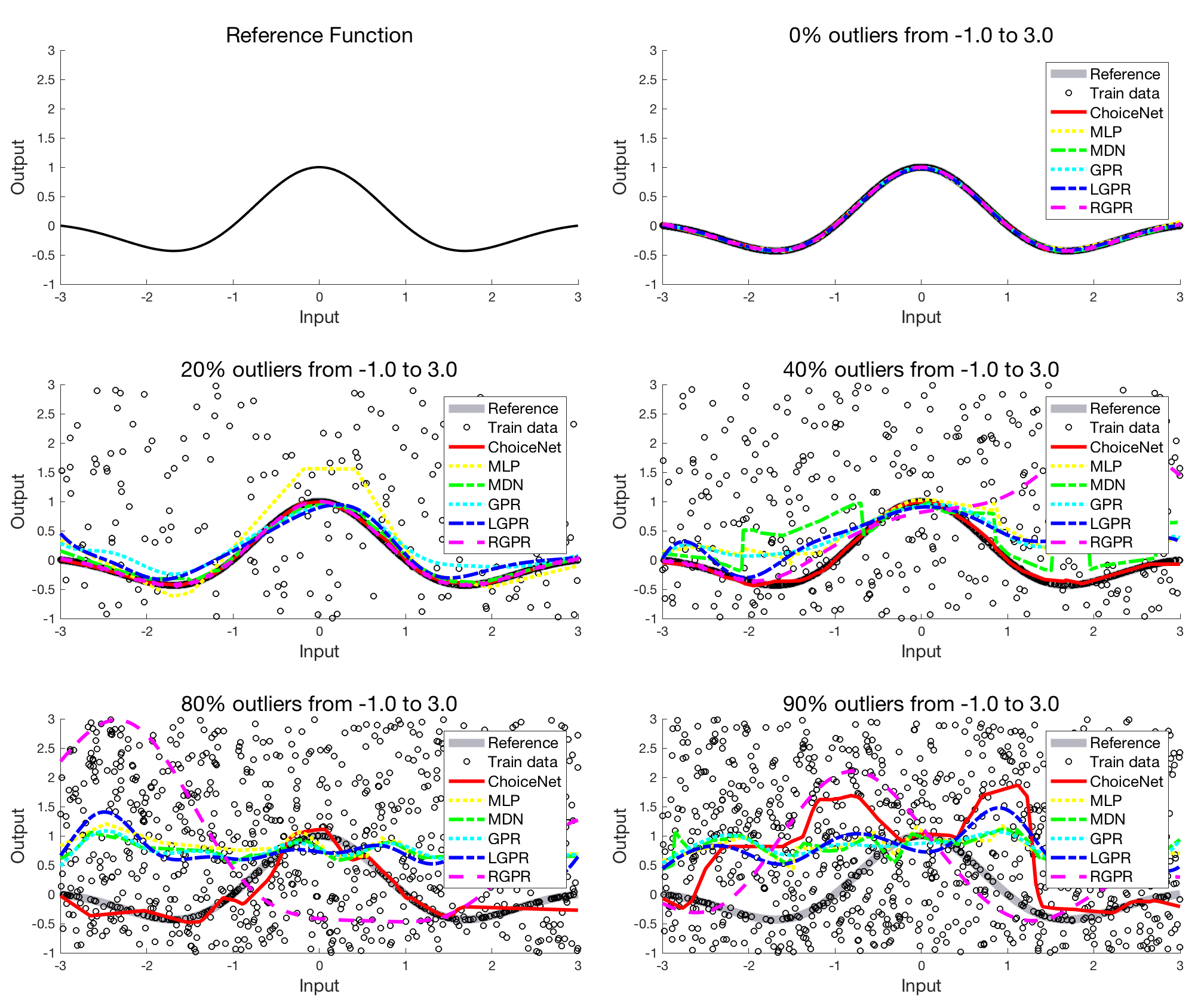
Figure 7: Reference function and fitting results of compared methods on different outlier rates, $0\%$,$20\%$ $40\%$, $80\%$, and $90\%$).

Table 4: The RMSEs of compared methods on synthetic toy examples

Outliers	ChoiceNet	MLP	GPR	LGPR	RGPR	MDN
$0\%$	$0.034$	$0.039$	$\bf{0.008}$	$0.022$	$0.017$	$0.028$
$20\%$	$0.022$	$0.413$	$0.280$	$0.206$	$\bf{0.013}$	$0.087$
$40\%$	$\bf{0.018}$	$0.452$	$0.447$	$0.439$	$1.322$	$0.565$
$60\%$	$\bf{0.023}$	$0.636$	$0.602$	$0.579$	$0.738$	$0.645$
$80\%$	$\bf{0.084}$	$0.829$	$0.779$	$0.777$	$1.523$	$0.778$

Boston Housing Dataset

Here, we used a real world dataset, a Boston housing price dataset, and checked the robustness of the proposed method and compared with standard multi-layer perceptrons with four different types of loss functions: standard $L2$-loss, $L1$-loss which is known to be robust to outliers, a robust loss (RL) function proposed in [21], and a leaky robust loss (LeakyRL) function. We further implement the leaky version of [21] in that the original robust loss function with Tukey’s biweight function discards the instances whose residuals exceed certain threshold.

Table 5: The RMSEs of compared methods on the Boston Housing Dataset

Outliers	ChoiceNet	$L2$	$L1$	RL	LeakyRL	MDN
$0\%$	$3.29$	3.22	$3.26$	$4.28$	$3.36$	$3.46$
$10\%$	3.99	$5.97$	$5.72$	$6.36$	$5.71$	$6.5$
$20\%$	4.77	$7.51$	$7.16$	$8.08$	$7.08$	$8.62$
$30\%$	5.94	$9.04$	$8.65$	$10.54$	$8.67$	$8.97$
$40\%$	6.80	$9.88$	$9.69$	$10.94$	$9.68$	$10.44$

Table 6: Average returns of compared methods on behavior cloning problems using MuJoCo

Outliers	HalfCheetah			Walker2d
	ChoiceNet	MDN	MLP	ChoiceNet	MDN	MLP
$10\%$	2068.14	192.53	852.91	2754.08	102.99	537.42
$20\%$	1498.72	675.94	372.90	1887.73	95.29	1155.80
$30\%$	2035.91	363.08	971.24	-267.10	-260.80	-728.39

Behavior Cloning Example

In this experiment, we apply ChoiceNet to behavior cloning tasks when given demonstrations with mixed qualities where the proposed method is compared with a MLP and a MDN in two locomotion tasks: HalfCheetah and Walker2d. The network architectures are identical to those in the synthetic regression example tasks. To evaluate the robustness of ChoiceNet, we collect demonstrations from both an expert policy and an adversarial policy where two policies are trained by solving the corresponding reinforcement learning problems using the state-of-the-art proximal policy optimization (PPO) [48]. For training adversarial policies for both tasks, we flip the signs of the directional rewards so that the agent gets incentivized by going backward. We evaluate the performances of the compared methods using $500$ state-action pairs with different mixing ratio and measure the average return over $100$ consecutive episodes. The results are shown in Table 6. In both cases, ChoiceNet outperforms compared methods by a significant margin. Additional behavior cloning experiments for autonomous driving can be found in the supplement material.

Autonomous Driving Experiment

In this experiment, we apply ChoiceNet to a autonomous driving scenario in a simulated environment. In particular, the tested methods are asked to learn the policy from driving demonstrations collected from both safe and careless driving modes. We use the same set of methods used for the previous task. The policy function is defined as a mapping between four dimensional input features consist of three frontal distances to left, center, and right lanes and lane deviation distance from the center of the lane to the desired heading. Once the desired heading is computed, the angular velocity of a car is computed by $10*(\theta_{\text{desired}}-\theta_{\text{current}})$ and the directional velocity is fixed to $10m/s$. The driving demonstrations are collected from keyboard inputs by human users. The objective of this experiment is to assess its performance on a training set generated from two different distributions. We would like to note that this task does not have a reference target function in that all demonstrations are collected manually. Hence, we evaluated the performances of the compared methods by running the trained policies on a straight track by randomly deploying static cars.

Table 7 and Table 8 indicate collision rates and RMS lane deviation distances of the tested methods, respectively, where the statistics are computed from $50$ independent runs on the straight lane by randomly placing static cars as shown in Figure 8. ChoiceNet clearly outperforms compared methods in terms of both safety (low collision rates) and stability (low RMS lane deviation distances).

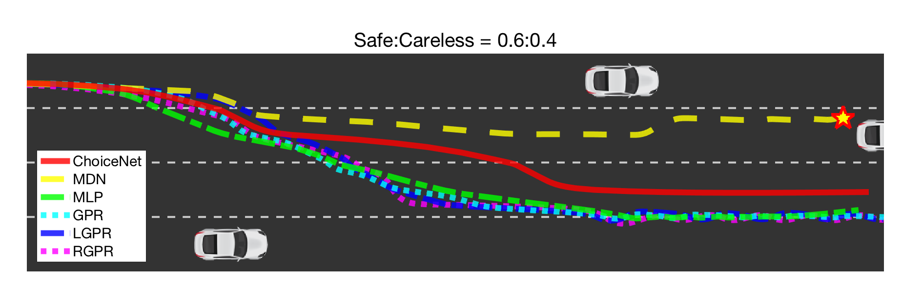
Figure 8: Resulting trajectories of compared methods trained with mixed demonstrations. (best viewed in color).

Table 7: Collision rates of compared methods on straight lanes.

Outliers	ChoiceNet	MDN	MLP	GPR	LGPR	RGPR
$0\%$	$\bf{0\%}$	$50.83\%$	$\bf{0\%}$	$0.83\%$	$4.17\%$	$3.33\%$
$10\%$	$\bf{0\%}$	$38.33\%$	$\bf{0\%}$	$2.5\%$	$1.67\%$	$4.17\%$
$20\%$	$\bf{0\%}$	$41.67\%$	$\bf{0\%}$	$7.5\%$	$6.67\%$	$10\%$
$30\%$	$\bf{0\%}$	$66.67\%$	$1.67\%$	$4.17\%$	$1.67\%$	$7.5\%$
$40\%$	$\bf{0.83\%}$	$35\%$	$3.33\%$	$6.67\%$	$6.67\%$	$24.17\%$

Table 8: Root mean square lane deviation distances (m) of compared methods on straight lanes.

Outliers	ChoiceNet	MDN	MLP	GPR	LGPR	RGPR
$0\%$	$0.314$	$0.723$	$\bf{0.300}$	$0.356$	$0.349$	$0.424$
$10\%$	$\bf{0.352}$	$0.387$	$0.438$	$0.401$	$0.446$	$0.673$
$20\%$	$\bf{0.349}$	$0.410$	$0.513$	$0.418$	$0.419$	$0.725$
$30\%$	$\bf{0.368}$	$\bf{0.368}$	$0.499$	$0.455$	$0.476$	$0.740$
$40\%$	$\bf{0.370}$	$0.574$	$0.453$	$0.453$	$0.453$	$0.636$

Here, we describe the features used for the autonomous driving experiments. As shown in the manuscript, we use a four dimensional feature, a lane deviation distance of an ego car, and three frontal distances to the closest car at left, center, and right lanes as shown in Figure 9. We upperbound the frontal distance to $40m$. Figure 10 and 10 illustrate manually collected trajectories of a safe driving mode and a careless driving mode.

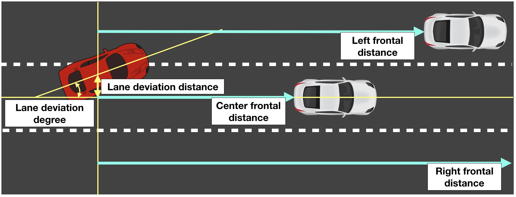
Figure 9: Descriptions of the featrues of an ego red car used in autonomous driving experiments.

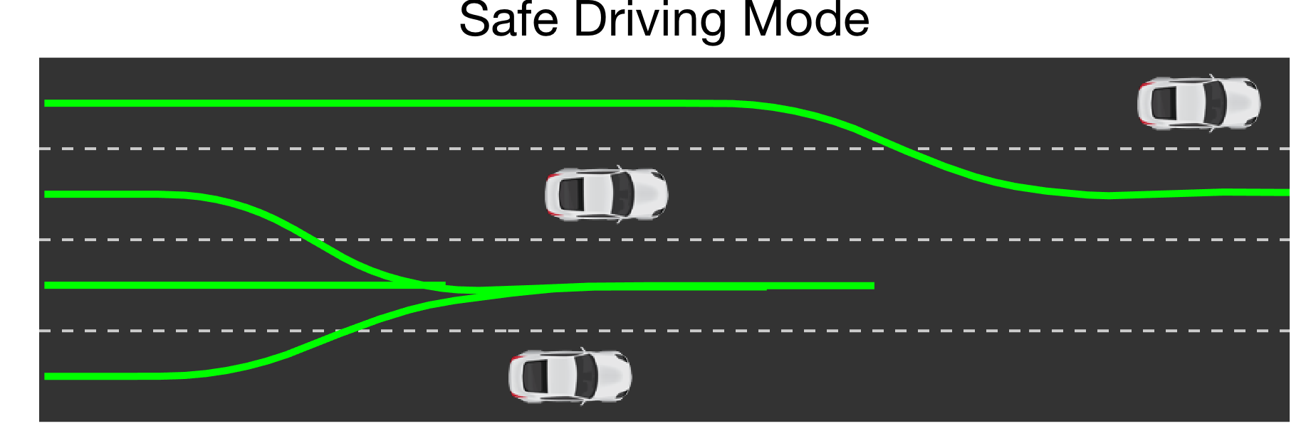
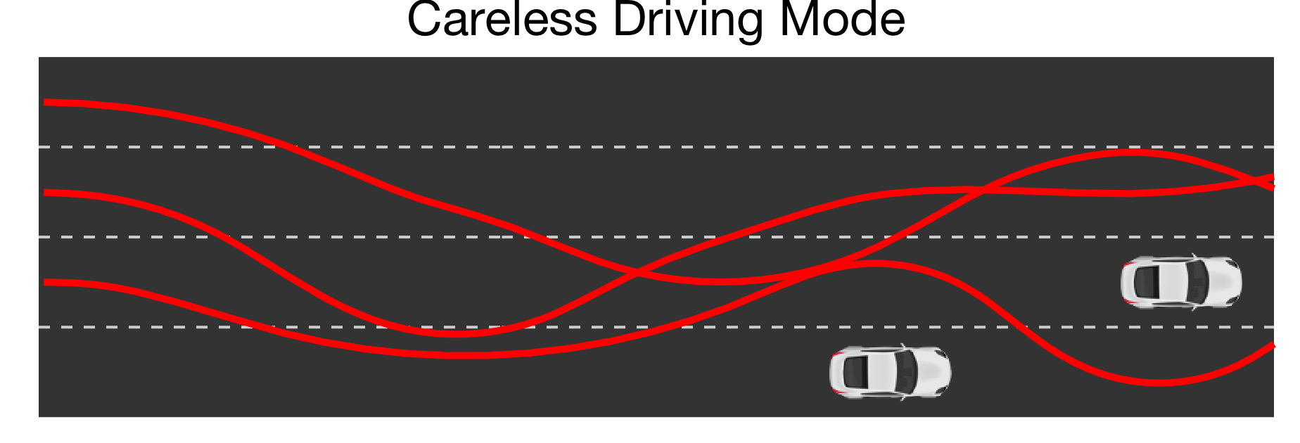
Figure 10: Manually collected trajectories of (a) safe driving mode and (b) careless driving mode. (best viewed in color).

B.2 Classification Tasks

Here, we conduct comprehensive classification experiments using MNIST, CIFAR-10, and Large Movie Review datasets to evaluate the performance of ChoiceNet on corrupt labels. For the image datasets, we followed two different settings to generate noisy datasets: one following the setting in [27] and the other from [12] which covers both symmetric and asymmetric noises. For the Large Movie Review dataset, we simply shuffle the labels to the other in that it only contains two labels.

MNIST

For MNIST experiments, we randomly shuffle a percentage of the labels with the corruption probability $p$ from $50\%$ to $95\%$ and compare median accuracies after five runs for each configuration following the setting in [27].

We construct two networks: a network with two residual blocks [49] with $3\times 3\times 64$ convolutional layers followed by a fully-connected layer with $256$ output units (ConvNet) and ChoiceNet with the same two residual blocks followed by the MCDN block (ConvNet+CN). We train each network for $50$ epochs with a fixed learning rate of 1e-5.

We train each network for $300$ epochs with a minibatch size of $256$. We begin with a learning rate of $0.1$, and it decays by $1/10$ after $150$ and $225$ epochs. We apply random horizontal flip and random crop with 4$-$pixel-padding and use a weight decay of $0.0001$ for the baseline network as [49].

Table 9: Test accuracies on the MNIST datasets with corrupt labels.

Corruption $p$	Configuration	Best	Last
50%	ConvNet	95.4	89.5
	ConvNet+Mixup	97.2	96.8
	ConvNet+CN	99.2	99.2
	MDN	97.7	97.7
80%	ConvNet	86.3	76.9
	ConvNet+Mixup	87.2	87.2
	ConvNet+CN	98.2	97.6
	MDN	85.2	78.7
90%	ConvNet	76.1	69.8
	ConvNet+Mixup	74.7	74.7
	ConvNet+CN	94.7	89.0
	MDN	61.4	50.2
95%	ConvNet	72.5	64.4
	ConvNet+Mixup	69.2	68.2
	ConvNet+CN	88.5	80.0
	MDN	31.2	25.9

The classification results are shown in Table 9 where ChoiceNet consistently outperforms ConvNet and ConvNet+Mixup by a significant margin, and the difference between the accuracies of ChoiceNet and the others becomes more clear as the corruption probability increases.

Here, we also present additional experimental results using the MNIST dataset on following three different scenarios:

1. Biased label experiments where we randomly assign the percentage of the training labels to label $0$.

2. Random shuffle experiments where we randomly replace the percentage of the training labels from the uniform multinomial distribution.

3. Random permutation experiments where we replace the percentage of the labels based on the label permutation matrix where we follow the random permutation in [22].

The best and final accuracies on the intact test dataset for biased label experiments are shown in Table 10. In all corruption rates, ChoiceNet achieves the best performance compared to two baseline methods. The learning curves of the biased label experiments are depicted in Figure 11. Particularly, we observe unstable learning curves regarding the test accuracies of ConvNet and Mixup. As training accuracies of such methods show stable learning behaviors, this can be interpreted as the networks are simply memorizing noisy labels. In the contrary, the learning curves of ChoiceNet show stable behaviors which clearly indicates the robustness of the proposed method.

The experimental results and learning curves of the random shuffle experiments are shown in Table 11 and Figure 12. The convolutional neural networks trained with Mixup show robust learning behaviors when $80\%$ of the training labels are uniformly shuffled. However, given an extremely noisy dataset ($90\%$ and $95\%$), the test accuracies of baseline methods decrease as the number of epochs increases. ChoiceNet shows outstanding robustness to the noisy dataset in that the test accuracies do not drop even after $50$ epochs for the cases where the corruption rates are below $90\%$. For the $95\%$ case, however, over-fitting is occured in all methods.

Table 12 and Figure 13 illustrate the results of the random permutation experiments. Specifically, we change the labels of randomly selected training data using a permutation rule: $(0,1,2,3,4,5,6,7,8,9)\to(7,9,0,4,2,1,3,5,6,8)$ following [22]. We argue that this setting is more arduous than the random shuffle case in that we are intentionally changing the labels based on predefined permutation rules.

Table 10: Test accuracies on the MNIST dataset with biased label.

Corruption $p$	Configuration	Best	Last
25%	ConvNet	95.4	89.5
	ConvNet+Mixup	97.2	96.8
	ChoiceNet	99.2	99.2
40%	ConvNet	86.3	76.9
	ConvNet+Mixup	87.2	87.2
	ChoiceNet	98.2	97.6
45%	ConvNet	76.1	69.8
	ConvNet+Mixup	74.7	74.7
	ChoiceNet	94.7	89.0
47%	ConvNet	72.5	64.4
	ConvNet+Mixup	69.2	68.2
	ChoiceNet	88.5	80.0

Table 11: Test accuracies on the MNIST dataset with corrupt label.

Corruption $p$	Configuration	Best	Last
50%	ConvNet	97.1	95.9
	ConvNet+Mixup	98.0	97.8
	ChoiceNet	99.1	99.0
80%	ConvNet	90.6	79.0
	ConvNet+Mixup	95.3	95.1
	ChoiceNet	98.3	98.3
90%	ConvNet	76.1	54.1
	ConvNet+Mixup	78.6	42.4
	ChoiceNet	95.9	95.2
95%	ConvNet	50.2	31.3
	ConvNet+Mixup	53.2	26.6
	ChoiceNet	84.5	66.0

Table 12: Test accuracies on the MNIST dataset with randomly permutated label.

Corruption $p$	Configuration	Best	Last
25%	ConvNet	94.4	92.2
	ConvNet+Mixup	97.6	97.6
	ChoiceNet	99.2	99.2
40%	ConvNet	77.9	71.8
	ConvNet+Mixup	84.0	83.0
	ChoiceNet	99.2	98.8
45%	ConvNet	68.0	61.4
	ConvNet+Mixup	68.9	55.8
	ChoiceNet	98.0	97.1
47%	ConvNet	58.2	53.9
	ConvNet+Mixup	60.2	53.4
	ChoiceNet	92.5	86.1

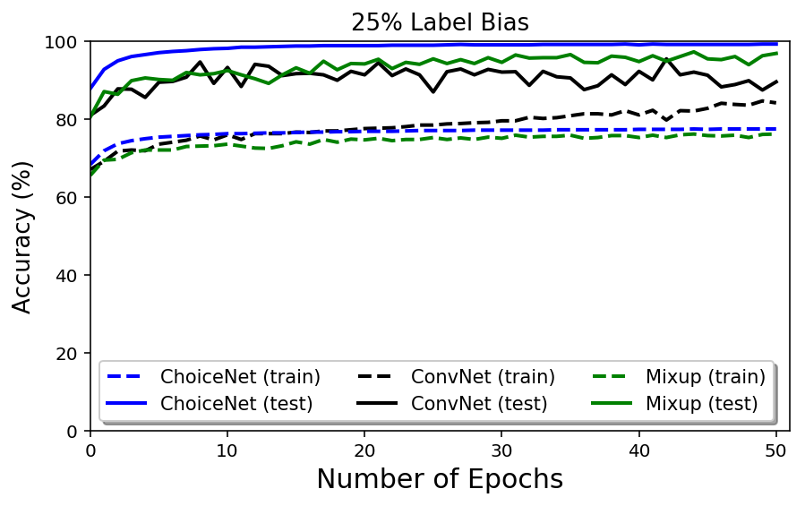
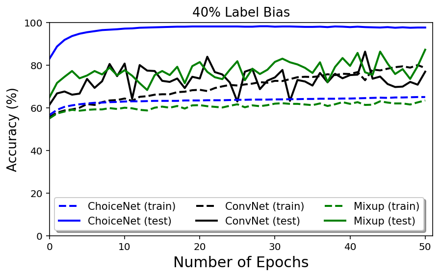
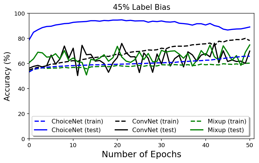
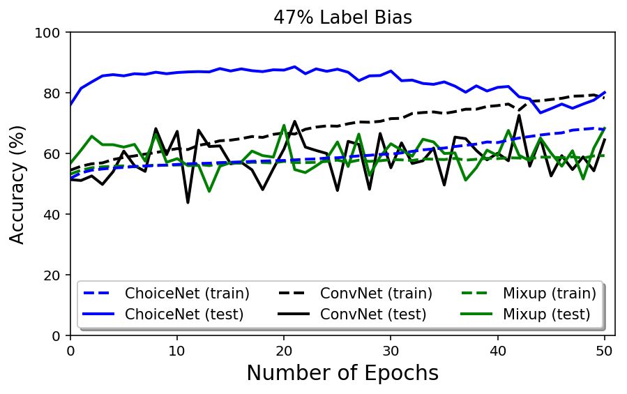
Figure 11: Learning curves of compared methods on random bias experiments using MNIST with different noise levels.

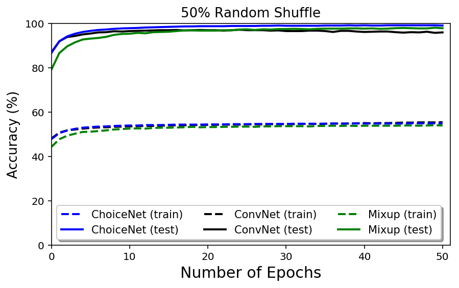
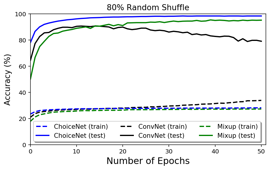
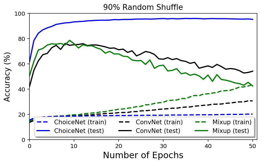
Figure 12: Learning curves of compared methods on random shuffle experiments using MNIST with different noise levels.

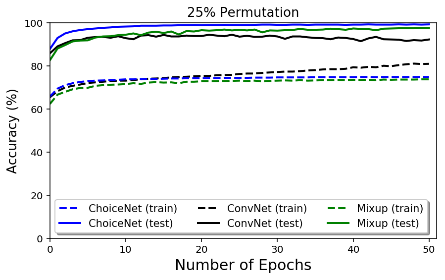
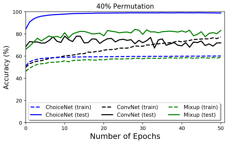
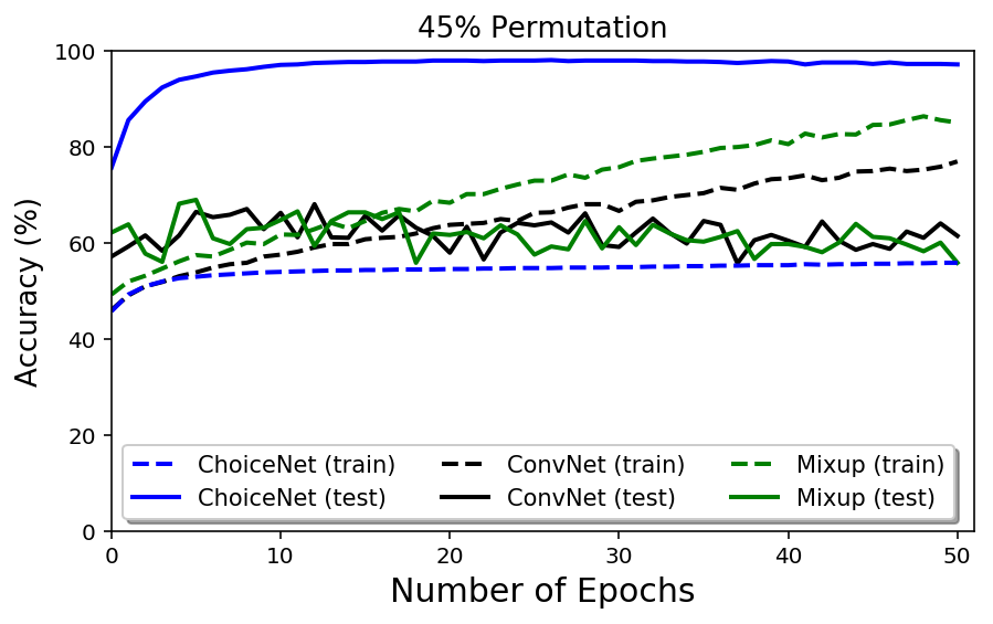
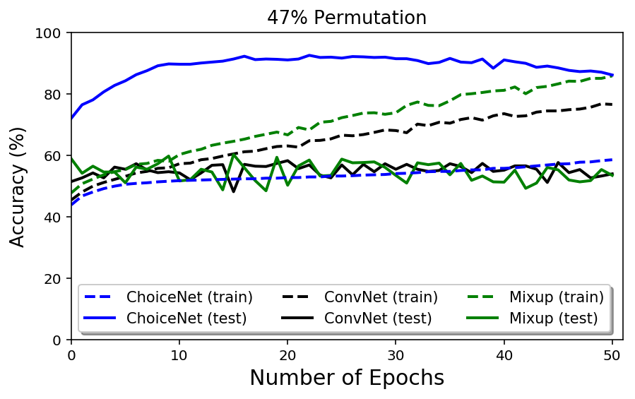
Figure 13: Learning curves of compared methods on random permutation experiments using MNIST with different noise levels.

CIFAR-10

When using the CIFAR-10 dataset, we followed two different settings from [27] and [12] for more comprehensive comparisons. Note that the setting in [12] incorporates both symmetric and asymmetric noises.

For the first scenario following [27], we apply symmetric noises to the labels and vary the corruption probabilities from $50\%$ to $80\%$. We compare our method with Mixup [27], VAT [28], and MentorNet [10]. We adopt WideResNet (WRN) [45] with $22$ layers and a widening factor of $4$. To construct ChoiceNet, we replace the last layer of WideResNet with a MCDN block. We set $K=3$, $\rho_{\text{max}}=0.95$, $\lambda_{\text{reg}}=0.0001$, and $\rho_{k},\pi_{k},\Sigma_{0}$ modules consist of two fully connected layers with $64$ hidden units and a ReLU activation function. We train each network for $300$ epochs with a minibatch size of $256$. We begin with a learning rate of $0.1$, and it decays by $1/10$ after $150$ and $225$ epochs. We apply random horizontal flip and random crop with 4$-$pixel-padding and use a weight decay of $0.0001$ for the baseline network as [49]. To train ChoiceNet, we set the weight decay rate to $1e-6$ and apply gradient clipping at $1.0$.

Table 13: Test accuracies on the CIFAR-10 datasets with symmetric noises.

Corruption $p$	Configuration	Accuarcy ($\%$)
50%	ConvNet	59.3
	ConvNet+CN	84.6
	ConvNet+Mixup	83.1
	ConvNet+Mixup+CN	87.9
	MentorNet	49.0
	VAT	71.6
	MDN	58.6
80%	ConvNet	27.4
	ConvNet+CN	65.2
	ConvNet+Mixup	62.9
	ConvNet+Mixup+CN	75.4
	MentorNet	21.4
	VAT	16.9
	MDN	22.7

Table 13 shows the test accuracies of compared methods under different symmetric corruptions probabilities. In all cases, ConvNet+CN outperforms the compared methods. We would like to emphasize that when ChoiceNet and Mixup [27] are combined, it achieves a high accuracy of $75\%$ even on the $80\%$ shuffled dataset. We also note that ChoiceNet (without Mixup) outperforms WideResNet+Mixup when the corruption ratio is over $50\%$ on the last accuracies.

We conduct additional experiments on the CIFAR-10 dataset to better evaluate the performance on both both symmetric and asymmetric noises following [12]: Pair-$45\%$, Symmetry-$50\%$, and Symmetry-$20\%$. Pair-$45\%$ flips $45\%$ of each label to the next label, e.g., randomly flipping $45\%$ of label $1$ to label $2$ and label $2$ to label $3$, and Symmetry-$50\%$ randomly assigns $50\%$ of each label to other labels uniformly. We implement the a $9$-layer CNN architecture following VAT [28] and Co-teaching [12] for fair and accurate evaluations and set other configurations such as the network topology and activations to be the same as [12]. We also copied some results in [12] for better comparisons. Here, we compared our method with MentorNet [10], Co-teaching [12], and F-correction [14].

Table 14: Test accuracies on the CIFAR-10 dataset with by symmetric and asymmetric noises.

	Pair-$45\%$	sym-$50\%$	sym-$20\%$
ChoiceNet	70.3	85.2	91.0
MentorNet	58.14	71.10	80.76
Co-teaching	72.62	74.02	82.32
F-correction	6.61	59.83	59.83
MDN	51.4	58.6	81.4

While our proposed method outperforms all compared methods on the symmetric noise settings, it shows the second best performance on asymmetric noise settings (Pair-$45\%$). This shows the weakness of the proposed method. In other words, as Pair-$45\%$ assigns $45\%$ of each label to its next label, the MCDN fails to correctly infer the dominant label distributions. However, we would like to note that Co-teaching [12] is complementary to our method where one can combine these two methods by using two ChoiceNets and update each network using Co-teaching. However, it is outside the scope of this paper.

Here, we also present detailed learning curves of the CIFAR-10 experiments while varying the noise level from $20\%$ to $80\%$ following the configurations in [27].

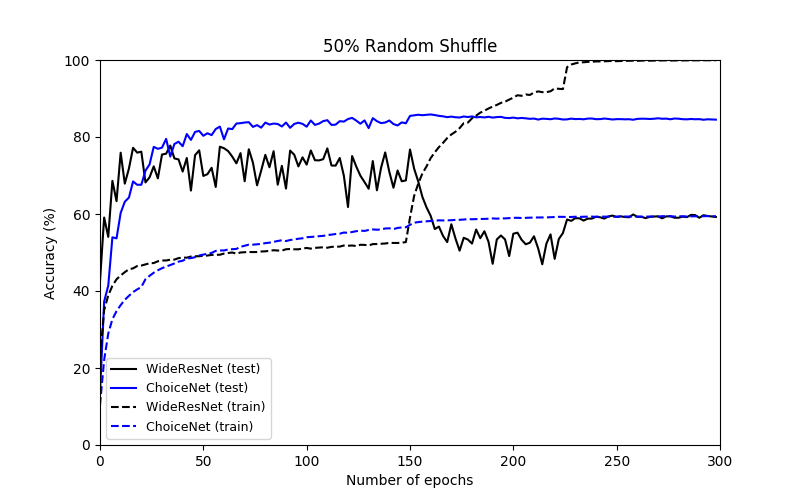
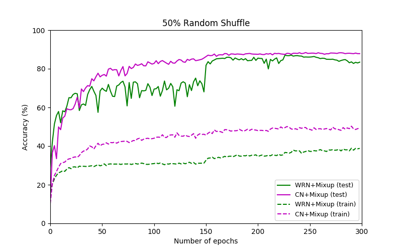
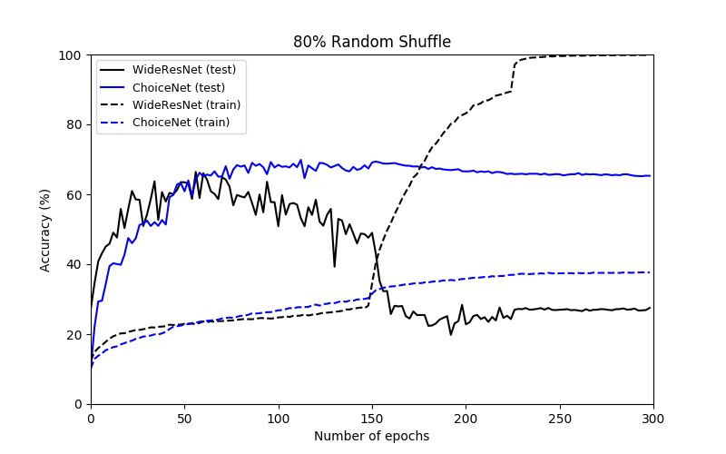
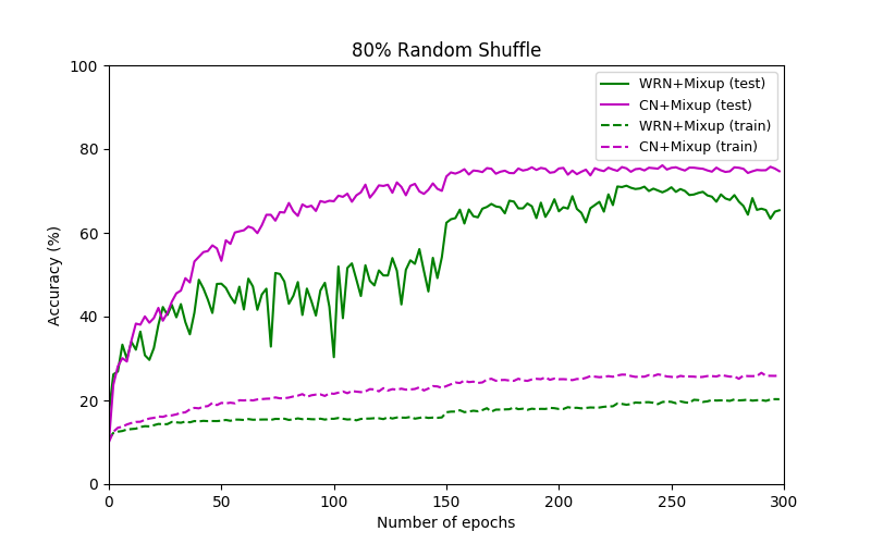
Figure 14: Learning curves of compared methods on CIFAR-10 experiments with different noise levels.

Large Movie Review Dataset

We also conduct a natural language processing task using a Large Movie Review dataset which consists of $25,000$ movie reviews for training and $25,000$ reviews for testing. Each movie review (sentences) is mapped to a $128$-dimensional embedding vector using a feed-forward Neural-Net Language Models [50]. We evaluated the robustness of the proposed method with Mixup [27], VAT [28], and naive MLP baseline by randomly flipping the labels with a corruption probability $p$. In all experiments, we used two hidden layers with $128$ units and ReLU activations. The test accuracies of the compared methods are shown in Table 15. ChoiceNet shows the superior performance in the presence of outliers where we observe that the proposed method can be used for NLP tasks as well.

Table 15: Test accuracies on the Large Movie Review dataset with different corruption probabilities.

Corruption $p$	$0\%$	$10\%$	$20\%$	$30\%$	$40\%$
ChoiceNet	79.43	79.50	78.66	77.1	73.98
Mixup	79.77	78.73	77.58	75.85	69.63
MLP	79.04	77.88	75.70	69.05	62.83
VAT	76.40	72.50	69.20	65.20	58.30

B.3 Ablation Study on MNIST

Above figures show the results of ablation study when varying the number of mixture $K$ and the expected measurement variance $\tau^{-1}$. Left two figures indicate test accuracies using the MNIST dataset where $90\%$ of train labels are randomly shuffled and right two figures are RMSEs using a synthetic one-dimensional regression problem in Section 4.1. We observe that having bigger $K$ is beneficial to the classification accuracies. In fact, the results achieved here with $K$ equals $15$ and $20$ are better than the ones reported in the submitted manuscript. $\tau^{-1}$ does not affect much unless it is exceedingly large.

References

- [1] Wei Bi, Liwei Wang, James T Kwok, and Zhuowen Tu, “Learning to predict from crowdsourced data.”, in UAI, 2014, pp. 82–91.
- [2] Chiyuan Zhang, Samy Bengio, Moritz Hardt, Benjamin Recht, and Oriol Vinyals, “Understanding deep learning requires rethinking generalization”, in Proc. of International Conference on Learning Representations, 2016.
- [3] Frank R Hampel, Elvezio M Ronchetti, Peter J Rousseeuw, and Werner A Stahel, Robust statistics: the approach based on influence functions, vol. 196, John Wiley & Sons, 2011.
- [4] Ishan Jindal, Matthew Nokleby, and Xuewen Chen, “Learning deep networks from noisy labels with dropout regularization”, in Proc. of IEEE International Conference onData Mining. IEEE, 2016, pp. 967–972.
- [5] Charles Blundell, Julien Cornebise, Koray Kavukcuoglu, and Daan Wierstra, “Weight uncertainty in neural networks”, in International Conference on Machine Learning (ICML), 2015.
- [6] Alhussein Fawzi, Seyed Mohsen Moosavi Dezfooli, and Pascal Frossard, “A geometric perspective on the robustness of deep networks”, IEEE Signal Processing Magazine, 2017.
- [7] Brian Paden, Michal Čáp, Sze Zheng Yong, Dmitry Yershov, and Emilio Frazzoli, “A survey of motion planning and control techniques for self-driving urban vehicles”, IEEE Transactions on Intelligent Vehicles, vol. 1, no. 1, pp. 33–55, 2016.
- [8] Varun Gulshan, Lily Peng, Marc Coram, Martin C Stumpe, Derek Wu, Arunachalam Narayanaswamy, Subhashini Venugopalan, Kasumi Widner, Tom Madams, Jorge Cuadros, et al., “Development and validation of a deep learning algorithm for detection of diabetic retinopathy in retinal fundus photographs”, Journal of the American Medical Association, vol. 316, no. 22, pp. 2402–2410, 2016.
- [9] AP and REUTERS, “Tesla working on ’improvements’ to its autopilot radar changes after model s owner became the first self-driving fatality.”, June 2016.
- [10] Lu Jiang, Zhengyuan Zhou, Thomas Leung, Li-Jia Li, and Li Fei-Fei, “Mentornet: Regularizing very deep neural networks on corrupted labels”, arXiv preprint arXiv:1712.05055, 2017.
- [11] Mengye Ren, Wenyuan Zeng, Bin Yang, and Raquel Urtasun, “Learning to reweight examples for robust deep learning”, in Proc. of International Conference on Machine Learning, 2018.
- [12] Bo Han, Quanming Yao, Xingrui Yu, Gang Niu, Miao Xu, Weihua Hu, Ivor Tsang, and Masashi Sugiyama, “Co-teaching: robust training deep neural networks with extremely noisy labels”, in Proc. of the Advances in Neural Information Processing Systems, 2018.
- [13] Eran Malach and Shai Shalev-Shwartz, “Decoupling" when to update" from" how to update"”, in Advances in Neural Information Processing Systems, 2017, pp. 961–971.
- [14] Giorgio Patrini, Alessandro Rozza, Aditya Krishna Menon, Richard Nock, and Lizhen Qu, “Making deep neural networks robust to label noise: a loss correction approach”, in Proc. of the Conference on Computer Vision and Pattern Recognition, 2017, vol. 1050, p. 22.
- [15] Jacob Goldberger and Ehud Ben-Reuven, “Training deep neural-networks using a noise adaptation layer”, in Proc. of International Conference on Learning Representations, 2017.
- [16] Sainbayar Sukhbaatar, Joan Bruna, Manohar Paluri, Lubomir Bourdev, and Rob Fergus, “Training convolutional networks with noisy labels”, arXiv preprint arXiv:1406.2080, 2014.
- [17] Alan Joseph Bekker and Jacob Goldberger, “Training deep neural-networks based on unreliable labels”, in Proc. of IEEE International Conference on Acoustics, Speech and Signal Processing. IEEE, 2016, pp. 2682–2686.
- [18] Dan Hendrycks, Mantas Mazeika, Duncan Wilson, and Kevin Gimpel, “Using trusted data to train deep networks on labels corrupted by severe noise”, arXiv preprint arXiv:1802.05300, 2018.
- [19] Andreas Veit, Neil Alldrin, Gal Chechik, Ivan Krasin, Abhinav Gupta, and Serge Belongie, “Learning from noisy large-scale datasets with minimal supervision”, in Conference on Computer Vision and Pattern Recognition, 2017.
- [20] Nagarajan Natarajan, Inderjit S Dhillon, Pradeep K Ravikumar, and Ambuj Tewari, “Learning with noisy labels”, in Proc. of the Advances in Neural Information Processing Systems, 2013, pp. 1196–1204.
- [21] Vasileios Belagiannis, Christian Rupprecht, Gustavo Carneiro, and Nassir Navab, “Robust optimization for deep regression”, in Proc. of the IEEE International Conference on Computer Vision, 2015, pp. 2830–2838.
- [22] Scott Reed, Honglak Lee, Dragomir Anguelov, Christian Szegedy, Dumitru Erhan, and Andrew Rabinovich, “Training deep neural networks on noisy labels with bootstrapping”, arXiv preprint arXiv:1412.6596, 2014.
- [23] Dong-Hyun Lee, “Pseudo-label: The simple and efficient semi-supervised learning method for deep neural networks”, in Workshop on Challenges in Representation Learning, ICML, 2013, vol. 3, p. 2.
- [24] Ian Goodfellow, Yoshua Bengio, Aaron Courville, and Yoshua Bengio, Deep learning, vol. 1, MIT press Cambridge, 2016.
- [25] Lingxi Xie, Jingdong Wang, Zhen Wei, Meng Wang, and Qi Tian, “Disturblabel: Regularizing cnn on the loss layer”, in Proc. of the IEEE Conference on Computer Vision and Pattern Recognition, 2016, pp. 4753–4762.
- [26] Yuji Tokozume, Yoshitaka Ushiku, and Tatsuya Harada, “Proc. of international conference on learning representations”, 2018.
- [27] Hongyi Zhang, Moustapha Cisse, Yann N Dauphin, and David Lopez-Paz, “mixup: Beyond empirical risk minimization”, in Proc. of International Conference on Learning Representations, 2017.
- [28] Takeru Miyato, Shin-ichi Maeda, Shin Ishii, and Masanori Koyama, “Virtual adversarial training: a regularization method for supervised and semi-supervised learning”, IEEE transactions on pattern analysis and machine intelligence, 2018.
- [29] Antti Tarvainen and Harri Valpola, “Mean teachers are better role models: Weight-averaged consistency targets improve semi-supervised deep learning results”, in Advances in neural information processing systems, 2017, pp. 1195–1204.
- [30] Samuli Laine and Timo Aila, “Temporal ensembling for semi-supervised learning”, in Proc. of International Conference on Learning Representations, 2017.
- [31] Xin Liu, Shaoxin Li, Meina Kan, Shiguang Shan, and Xilin Chen, “Self-error-correcting convolutional neural network for learning with noisy labels”, in Proc. of IEEE International Conference on Automatic Face & Gesture Recognition. IEEE, 2017, pp. 111–117.
- [32] Aritra Ghosh, Himanshu Kumar, and PS Sastry, “Robust loss functions under label noise for deep neural networks.”, in Proc. of the AAAI Conference on Artificial Intelligence, 2017, pp. 1919–1925.
- [33] Carl Edward Rasmussen, “Gaussian processes for machine learning”, 2006.
- [34] Edwin V Bonilla, Kian M Chai, and Christopher Williams, “Multi-task gaussian process prediction”, in Proc. of the Advances in Neural Information Processing Systems, 2008, pp. 153–160.
- [35] Sungjoon Choi, Kyungjae Lee, and Songhwai Oh, “Robust learning from demonstration using leveraged Gaussian processes and sparse constrained opimization”, in Proc. of the IEEE International Conference on Robotics and Automation (ICRA). May 2016, IEEE.
- [36] Peter J Huber, Robust statistics, Springer, 2011.
- [37] Diederik P Kingma, “Variational inference & deep learning: A new synthesis”, University of Amsterdam, 2017.
- [38] Christopher M Bishop, “Mixture density networks”, 1994.
- [39] Kaiming He, Xiangyu Zhang, Shaoqing Ren, and Jian Sun, “Deep residual learning for image recognition”, in Proc. of the IEEE conference on Computer Vision and Pattern Recognition, 2016, pp. 770–778.
- [40] Omer Levy and Yoav Goldberg, “Neural word embedding as implicit matrix factorization”, in Advances in neural information processing systems, 2014, pp. 2177–2185.
- [41] Alex Kendall and Yarin Gal, “What uncertainties do we need in bayesian deep learning for computer vision?”, in Advances in Neural Information Processing Systems, 2017, pp. 5580–5590.
- [42] Sungjoon Choi, Kyungjae Lee, Sungbin Lim, and Songhwai Oh, “Uncertainty-aware learning from demonstration using mixture density networks with sampling-free variance modeling”, arXiv preprint arXiv:1709.02249, 2017.
- [43] M Bishop Christopher, PATTERN RECOGNITION AND MACHINE LEARNING., Springer-Verlag New York, 2016.
- [44] Alex Kendall and Yarin Gal, “What uncertainties do we need in Bayesian deep learning for computer vision?”, in Proc. of the Advances in Neural Information Processing Systems, 2017.
- [45] Sergey Zagoruyko and Nikos Komodakis, “Wide residual networks”, in BMVC, 2016.
- [46] Carl E Rasmussen and Zoubin Ghahramani, “Infinite mixtures of gaussian process experts”, in Advances in Neural Information Processing Systems, 2002, pp. 881–888.
- [47] Bo Dai, Bo Xie, Niao He, Yingyu Liang, Anant Raj, Maria-Florina F Balcan, and Le Song, “Scalable kernel methods via doubly stochastic gradients”, in Proc. of the Advances in Neural Information Processing Systems, 2014, pp. 3041–3049.
- [48] John Schulman, Filip Wolski, Prafulla Dhariwal, Alec Radford, and Oleg Klimov, “Proximal policy optimization algorithms”, arXiv preprint arXiv:1707.06347, 2017.
- [49] Kaiming He, Xiangyu Zhang, Shaoqing Ren, and Jian Sun, “Deep residual learning for image recognition”, in Proceedings of the IEEE conference on computer vision and pattern recognition, 2016, pp. 770–778.
- [50] Yoshua Bengio, Réjean Ducharme, Pascal Vincent, and Christian Jauvin, “A neural probabilistic language model”, Journal of machine learning research, vol. 3, no. Feb, pp. 1137–1155, 2003.