Simulating squirmers with multiparticle collision dynamics

Abstract

Multiparticle collision dynamics is a modern coarse-grained simulation technique to treat the hydrodynamics of Newtonian fluids by solving the Navier-Stokes equations. Naturally, it also includes thermal noise. Initially it has been applied extensively to spherical colloids or bead-spring polymers immersed in a fluid. Here, we review and discuss the use of multiparticle collision dynamics for studying the motion of spherical model microswimmers called squirmers moving in viscous fluids.

1 Introduction

Recently, there has been a great interest in understanding the physical principles of the locomotion mechanisms of microswimmers. Important examples are biological microorganisms such as bacteria, sperm cells or algae, and artificial self-propelled swimmers such as active colloids Zottl2016 ; Bechinger2016 or active emulsion droplets Maass2016 . Their locomotion is mainly governed by low Reynolds number hydrodynamics and thermal or biological noise. While swimming speed and flow fields of a single noiseless microswimmer in a bulk fluid may be calculated analytically in some simple cases by solving Stokes equations Taylor51 ; Lighthill52 ; Blake71 ; Najafi2004 ; Avron2005 , analytical methods are less suitable for swimmers in complex environments, in the presence of other swimmers, or when Brownian fluctuations become important. Hence several numerical methods are used nowadays to overcome these limitations. Very succesful tools are coarse-grained hydrodynamic simulation methods such as lattice Boltzmann (LB), dissipative particle dynamics (DPD), and multiparticle collision dynamics (MPCD) – a special version of which is stochastic rotation dynamics (SRD). These methods allow to simulate the time evolution of one or many swimmers, in bulk as well as in confinement. While MPCD and DPD are particle-based methods and naturally include thermal fluctuations, LB is based on the time evolution of smooth velocity distribution functions and noise may be included on top.

In particular, MPCD has been used extensively in the last decade to simulate the dynamics and flow fields of various nano-and microswimmers like a Taylor sheet Muench2016 , artificial nano- and microswimmers Rueckner07 ; Tao08 ; Tao09 ; Tao09b ; Thakur10 ; Thakur10b ; Thakur11 ; Thakur11b ; Yang11 ; Thakur12 ; Huang12 ; deBuyl13 ; Kapral13 ; Yang13 ; Yang2014 ; Wagner2017 , sperm cells, flagella, cilia, and self-propelled rods YangB08 ; Elgeti08 ; Elgeti09 ; Elgeti10 ; YangB10 ; Reigh12 ; Reigh13 ; YangB13 ; Elgeti13 ; Yang2014b ; Agrawal2018 , dumbbell swimmers Schwarzendahl2017 , swimming bacteria Hu2015 ; Hu2015b ; Zottl2017 , and the complicated motion of the parasite African Trypanosome Babu12b ; Heddergott12 ; Alizadehrad2015 and bacterial swarmer cells Eisenstecken2016 . At present a very popular spherical model swimmer is the so-called squirmer. Its motion has recently been modeled with MPCD and it has been used to explore generic features of microswimmers Downton09 ; Goetze10 ; Zottl2012 ; Zottl2014 ; Schaar2015 ; Blaschke2016 ; Theers2016 ; Kuhr2017 ; Ruehle2018 . In this paper we will summarize the details how the squirmer is implemented and simulated with MPCD.

We first introduce the basics of the MPCD method in section 2 and discuss the squirmer model briefly in section 3. We then explain in detail how the motion of the squirmer can be coupled to the MPCD fluid using a hybrid molecular dynamics – multiparticle collision dynamics (MD-MPCD) scheme in section 4. We then present results for swimming in a narrow slit geometry in section 5, and finish with a conclusion in section 6.

2 Multiparticle collision dynamics

Multiparticle collision dynamics (MPCD) is a coarse-grained solver of the Navier-Stokes equations Kapral08 ; Gompper08 , which naturally includes thermal fluctuations because it simulates the fluid explicitly via pointlike, effective fluid particles kept at temperature $T_{0}$. Transport coefficients such as the shear viscosity $\eta$ can be calculated analytically for a wide range of simulation parameters but depend on the particular collision rule between fluid particles Gompper08 .

The MPCD method was originally proposed by Malevanets and Kapral and termed stochastic rotation dynamics (SRD) Malevanets99 ; Malevanets00 . The fluid is modeled by $N_{p}$ effective fluid particles, which are pointlike and have mass $m_{0}$. They perform alternating streaming and collision steps and thereby solve the Navier-Stokes equations on a coarse-grained level since the collision step preserves local momentum. Initially, the particles are randomly placed in the simulation domain at initial positions $\mathbf{r}_{i}(t=0)$ and at velocities $\mathbf{v}_{i}(t=0)$ that are drawn from a normal distribution with zero mean and standard deviation $\sigma_{0}=\sqrt{k_{B}T_{0}/m_{0}}$.

In the streaming step [see Fig. 1(a)] the fluid particles are moved ballistically for a time $\Delta t$ such that their positions are updated to

$$\mathbf{r}_{i}(t+\Delta t)=\mathbf{r}_{i}(t)+\mathbf{v}_{i}(t)\Delta t.$$ (1)

Noteworthy, here $\Delta t$ is a simulation parameter, which determines fluid properties such as the viscosity. This is in contrast to molecular dynamics (MD) simulations, where $\Delta t$ only determines the accuracy of a simulation run. Typically, $\Delta t=10^{-2}-10^{0}$ in MPCD units. After the streaming step all the fluid particles are sorted into cubic cells with edge length $a_{0}$. To perform the collision step, all particles in a cell interact with each other and their velocities are updated to [see also Fig. 1(b)]

$$\mathbf{v}_{i}(t+\Delta t)=\mathbf{u}_{\xi}(t)+\bm{\Xi}(\mathbf{r}_{j}(t),\mathbf{v}_{j}(t)).$$ (2)

Here $\xi=1,\dots,N_{c}$ ist the cell index, $N_{c}$ is the total number of cells, and $\mathbf{u}_{\xi}(t)$ is the average particle velocity in cell $\xi$. The collision operator $\bm{\Xi}(\mathbf{r}_{j}(t),\mathbf{v}_{j}(t))$ in general depends on positions and velocities of the fluid particles in cell $\xi$. It has to be chosen such that momentum is conserved locally in each cell, in order to reproduce a flow field, which solves the Navier-Stokes equations. Depending on its concrete realization it either conserves energy or keeps temperature and thus the mean kinetic energy constant.

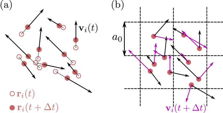
Figure 1: Sketch of the MPCD method. (a) Streaming step: Pointlike fluid particles move ballistically for a time $\Delta t$ with velocities $\mathbf{v}_{i}$. (b) Collision step: Particles are sorted into cubic cells of edge length $a_{0}$ and exchange momentum with other particles in the cell such that the total momentum is conserved.

In the original SRD method the fluid particles are part of a microcanonical ensemble and both momentum and energy is conserved locally. The collision operator reads

$$\bm{\Xi}=\mathcal{R}_{\alpha}(\vec{v}_{i}-\vec{u}_{\xi}),$$ (3)

where $\mathcal{R}_{\alpha}$ is a rotation operator, which rotates the relative velocities $\vec{v}_{i}-\vec{u}_{\xi}$ about a randomly chosen axis by a fixed angle $\alpha$. In order to fulfill Galilean invariance but also to reduce memory effects and correlations in the collision step, the cell grid is shifted randomly at each time step Ihle03 by a random vector $\mathbf{s}=\{s_{1},s_{2},s_{3}\}$, where the components $s_{i}$ are drawn from a uniform distribution $s_{i}\in[-a_{0}/2,a_{0}/2]$.

In their original paper Malevanets and Kapral showed Malevanets99 that by averaging out the particle dynamics on short length and time scales using a Chapman-Enskog expansion of the corresponding Boltzmann equation, the Navier-Stokes equations can be derived. Furthermore, the $\mathcal{H}$-theorem guarantees fluid relaxation towards equilibrium. The authors also demonstrated that the number of fluid particles per cell is Poisson distributed and the fluid particle velocity distribution converges fast towards a Maxwell-Boltzmann distribution. In addition, transport coefficients like the fluid viscosity can be calculated from the relevant model parameters $m_{0}$, $a_{0}$, $T_{0}$, $\gamma$, $\alpha$ and $\Delta t$ Malevanets99 ; Malevanets00 ; Ihle01 ; Ihle03 ; Tuezel03 ; Pooley05 ; Tuezel06 , where $\gamma=\sum_{\xi=1}^{N_{c}}n_{\xi}/N_{c}$ is the average number of fluid particles $n_{\xi}$ per cell.

Noguchi et al. developed alternative collision operators for MPCD fluids. They use a Langevin or Anderson thermostat to keep temperature constant but also to conserve momentum locally Noguchi07 ; Noguchi08 . Thus, a canonical ensemble of fluid particles is modeled, where energy is conserved on average. An advantage of these alternative collision rules is that local angular momentum conservation, which is missing in the original SRD formulation, can be included in a rather simple way. Although angular momentum conservation does not directly alter the Navier Stokes equations, it ensures that the stress tensor is symmetric, as it should be for the Newtonian fluid with its isotropy. Indeed, it has been shown that neglecting angular momentum conservation in the fluid may lead to incorrect physical effects Goetze07 . One popular approach for the collision operator is to use the Anderson thermostat and, in addition, conserve angular momentum. This type of collision rule is abbreviated by MPC-AT+a Noguchi07 . It has widely been used to study the dynamics of squirmers in MPCD fluids Goetze10 ; Zottl2012 ; Zottl2014 ; Schaar2015 ; Blaschke2016 ; Kuhr2017 ; Ruehle2018 .

3 Squirmer model

The squirmer is a simple spherical model swimmer. In its simplest form, a single parameter allows to tune the flow field initiated by the squirmer in the surrounding fluid. Thereby it mimics typical types of microswimmers ranging from pushers via neutral swimmer to pullers. The squirmer has been introduced originally as a model for ciliated microorganisms such as the spherical Volvox or the elongated Opalina Lighthill52 ; Blake71 . Their cell bodies are covered entirely by synchronously beating cilia, which propel them forward by propagating so-called metachronal waves along the cell surface Brennen77 . After averaging over a full beating cycle, characterized by a power stroke and recovery stroke, the resulting net flow close to the surface is nonzero. To account for these flows, the squirmer model was developed by Lighthill Lighthill52 and extended by Blake Blake71 . Cilia-induced flows close to the surface of the swimmer is here modeled by an effective slip velocity $\mathbf{v}_{s}$ directly at the surface of the sphere. Considering only axisymmetric flows, the time-dependent surface velocity fields in spherical coordinates read

$$\mathbf{v}_{s}(\theta,t)=v_{\theta}(\theta,t)\mathbf{e}_{\theta}+v_{r}(\theta,t)\mathbf{e}_{r}.$$ (4)

Without any thermal noise, a squirmer in bulk simply swims along its symmetry axis $\mathbf{e}$, and $\theta$ is the angle between this axis and the point $\vec{r}_{s}$ on the surface [see Fig. 2(a)]. The surface velocities can be expanded in Legendre polynomials $P_{n}$,

$$\begin{split}v_{\theta}(\theta,t)=&\sum_{n}A_{n}(t)P_{n}(\cos\theta)\\ v_{r}(\theta,t)=&\sum_{n}B_{n}(t)V_{n}(\cos\theta),\end{split}$$ (5)

where

$$V_{n}(\cos\theta)=\frac{2\sin\theta}{n(n+1)}\frac{\mathrm{d}P_{n}(\cos\theta)}{\mathrm{d}\cos\theta}.$$ (6)

The expansion coefficients $A_{n}$ and $B_{n}$ are sometimes called surface velocity modes. Solving the governing equations of low-Reynolds-number hydrodynamics, the Stokes equations Kim ; Happel , together with the boundary conditions [Eq. (5)] gives analytic expressions for the flow fields created by a squirmer in the surrounding fluid.

In many cases the surface velocity is assumed to be only tangential to the squirmer surface and time-independent. This describes in a good approximation the hydrodynamic flows close to spherical artificial microswimmers. Examples are active colloids Zottl2016 ; Bechinger2016 and droplets Schmitt13 ; Schmitt2016 ; Maass2016 which move themselves forward realizing static tangential stresses close to their surface, for example induced by self-phoretic mechanisms or self-induced Marangoni flows, respectively. Other examples are biological microswimmers such as Paramecia Ishikawa06b or Volvox Pedley2016 which propel themselves by synchronously beating thousands of tiny cilia attached to their surface. Averaged over a beating cycle, they induce strong tangential flows to move forward. Setting $v_{r}(\theta,t)=0$, the velocity field $\mathbf{v}(\mathbf{r})$ around a squirmer of radius $R$ with orientation $\mathbf{e}$ and located at position $\mathbf{r}_{0}$ can be calculated to Ishikawa06

$$\begin{split}&\mathbf{v}(\mathbf{r})=-\frac{1}{3}\frac{R^{3}}{r^{3}}B_{1}\mathbf{e}+\frac{R^{3}}{r^{3}}B_{1}(\mathbf{e}\cdot\hat{\mathbf{r}})\hat{\mathbf{r}}\\ &+\sum_{n=2}^{\infty}\left(\frac{R^{n+2}}{r^{n+2}}-\frac{R^{n}}{r^{n}}\right)B_{n}P_{n}(\mathbf{e}\cdot\hat{\mathbf{r}})\hat{\mathbf{r}}\\ &+\sum_{n=2}^{\infty}\left(\frac{n}{2}\frac{R^{n+2}}{r^{n+2}}-\left(\frac{n}{2}-1\right)\frac{R^{n}}{r^{n}}\right)B_{n}W_{n}(\mathbf{e}\cdot\hat{\mathbf{r}})\left[(\mathbf{e}\cdot\hat{\mathbf{r}})\hat{\mathbf{r}}-\mathbf{e}\right].\end{split}$$ (7)

Here $r=|\mathbf{r}-\mathbf{r}_{0}|$ is the distance from the squirmer center, $\hat{\mathbf{r}}=(\mathbf{r}-\mathbf{r}_{0})/r$ is the radial unit vector, and

$$W_{n}(\mathbf{e}\cdot\hat{\mathbf{r}})=W_{n}(\cos\theta)=\frac{2}{n(n+1)}\frac{\mathrm{d}P_{n}(\cos\theta)}{\mathrm{d}\cos\theta}$$ (8)

with $\mathbf{e}\cdot\hat{\mathbf{r}}=\cos\theta$.

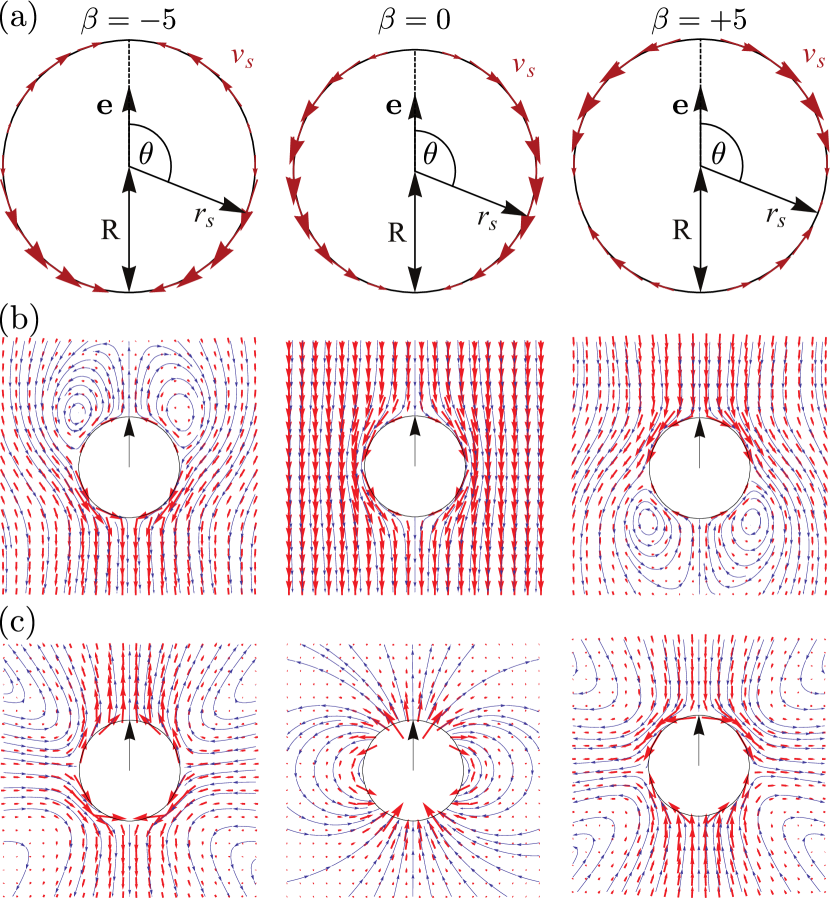
Figure 2: The squirmer model. (a) Axisymmetric surface velocity profile $\mathbf{v}_{s}(\theta)$ for a pusher ($\beta=-5$), a neutral squirmer ($\beta=0$) and a puller ($\beta=+5$). (b) Corresponding velocity fields (red) and stream lines (blue) in the frame moving with the swimmer. (c) Velocity fields (red) and stream lines (blue) in the lab frame.

The swimming speed $v_{0}$ of a noiseless squirmer in bulk solely depends on the first mode $B_{1}$ Lighthill52 ,

$$v_{0}=\frac{2}{3}B_{1},$$ (9)

and its velocity is constant, $\vec{V}_{0}=v_{0}\mathbf{e}$. It can be shown that the velocity of a sphere with tangential surface velocity $\vec{v}_{s}$ is equivalent to the average velocity on the surface Anderson1989 ; Stone96 ,

$$\vec{V}_{0}=-\frac{1}{4\pi R^{2}}\int_{S}\vec{v}_{s}\mathrm{d}S.$$ (10)

Indeed, it can be shown directly that only the first mode gives a nonzero contribution to the integral resulting in Eq. (9).

It is interesting to have a closer look at the flow field presented in Eq. (7), in particular at the behavior far away from the squirmer. The flow field created by the first mode $B_{1}$ is that of a source dipole. It decays as $\sim r^{-3}$ and is often the dominant contribution for spherical microswimmers Zottl2016 . The flow field created by the second mode $B_{2}$ is a force dipole field. It decays as $\sim r^{-2}$ and is the dominant field far away from the squirmer, because all other modes $B_{i}$ with $i\geqslant 3$ decay faster, see Eq. (7). For $B_{2}<0$ the far-field is the same as for a so-called pusher (or contractile swimmer) and for $B_{2}>0$ a so-called puller (or extensile swimmer) is realized. Typical pushers have the propelling apparatus at the back of their cell bodies, as observable in many bacteria or sperm cells. In contrast, pullers like Chlamydomonas have their flagella in front of the cell body. By tuning $B_{2}$, the squirmer can therefore be used as a simple model to capture different types of swimmers: pushers ($B_{2}<0$), pullers ($B_{2}>0$), and source-dipole swimmers ($B_{2}=0$).

In order to capture the flow fields of microswimmers in leading order correctly, it is sufficient to take the first two modes $B_{1}$ and $B_{2}$ into account. Experiments with active emulsion droplets have indeed demonstrated that the flow field can be approxiamted by these two modes only Thutupalli11 . The flow field of a swimming Paramecium has been measured as well. It can also be approximated well by considering only the leading modes with $B_{1}$ being the dominant mode Ishikawa06b .

Therefore, in numerical simulations the squirmer is very often used in its simplest form, only taking the first two modes into account. The resulting surface velocity field reads

$$\mathbf{v}_{s}(\mathbf{r}_{s},\mathbf{e})=B_{1}\left(1+\beta(\mathbf{e}\cdot\hat{\mathbf{r}}_{s})\right)\left[(\mathbf{e}\cdot\hat{\mathbf{r}}_{s})\hat{\mathbf{\mathbf{r}}}_{s}-\mathbf{e}\right]\,.$$ (11)

Here, $\hat{\mathbf{r}}_{s}=\mathbf{r}_{s}/R$ is the radial unit vector pointing from the squirmer center to its surface and the squirmer parameter $\beta$,

$$\beta=\frac{B_{2}}{B_{1}},$$ (12)

quantifies the leading-order flow field: pushers ($\beta<0$), pullers ($\beta>0$), and source-dipole swimmers ($\beta=0$). Figure 2(a) shows a sketch of squirmers and their surface velocity fields for $\beta=-5$, $\beta=0$, and $\beta=+5$. Its dimensionless velocity field $\mathbf{v}(\mathbf{r},\mathbf{e})/B_{1}$ generated in the surrounding fluid can then be written as

$$\begin{split}\frac{\mathbf{v}(\mathbf{r})}{B_{1}}=&\frac{R^{3}}{r^{3}}\left((\mathbf{e}\cdot\hat{\mathbf{r}})\hat{\mathbf{r}}-\frac{1}{3}\mathbf{e}\right)\\ &+\beta\left(\frac{R^{4}}{r^{4}}-\frac{R^{2}}{r^{2}}\right)\frac{1}{2}\left(-1+3(\mathbf{e}\cdot\hat{\mathbf{r}})^{2}\right)\hat{\mathbf{r}}\\ &+\beta\frac{R^{4}}{r^{4}}(\mathbf{e}\cdot\hat{\mathbf{r}})\left[(\mathbf{e}\cdot\hat{\mathbf{r}})\hat{\mathbf{r}}-\mathbf{e}\right],\end{split}$$ (13)

In leading order a force dipole field occurs,

$$\frac{\mathbf{v}_{D}(\mathbf{r})}{B_{1}}=-\frac{\beta}{2}\frac{R^{2}}{r^{2}}\left[-1+3(\mathbf{e}\cdot\hat{\mathbf{r}})^{2}\right]\hat{\mathbf{r}},$$ (14)

where the strength of the field is set by the squirmer parameter $\beta$ multiplied with the surface area of the sphere $\sim R^{2}$. Similarly, the mode $B_{1}$ is related to the source-dipole,

$$\frac{\mathbf{v}_{SD}(\mathbf{r})}{B_{1}}=\frac{R^{3}}{r^{3}}\left((\mathbf{e}\cdot\hat{\mathbf{r}})\hat{\mathbf{r}}-\frac{1}{3}\mathbf{e}\right)\,,$$ (15)

which scales with the volume of the squirmer $\sim R^{3}$. Figures 2(b) and (c) show flow fields (red) and stream lines (blue) around pushers ($\beta<0$), pullers ($\beta>0$), and neutral squirmers ($\beta=0$) both in the swimmer (b) and the lab frame (c).

Building on the pioneering work of Lighthill Lighthill52 and Blake Blake71 , the squirmer was rediscovered by Pedley and co-workers. They used the squirmer to model the nutrient uptake of spherical microswimmers Magar03 ; Magar05 , the flow around swimming Volvox Pedley2016 , the pairwise hydrodynamic interaction between two squirmers and between two Paramecia Ishikawa06 ; Ishikawa06b ; Giacche10 , collective motion of squirmers in bulk Ishikawa07b ; Ishikawa07c ; Ishikawa08b ; Ishikawa10 ; Evans11 , in flow Ishikawa07a ; Ishikawa12 ; Pagonabarraga13 , and in a monolayer Ishikawa08a . Within the last ten years the squirmer was also used extensively by other groups to study the persistent random walk of Brownian squirmers Downton09 , optimal swimming efficiency and feeding Michelin10 ; Michelin11 , finite Reynolds number locomotion Wang12a ; Khair2014 ; Chisholm2016 ; Li2016 , unsteady squirming Wang12b , the motion in a stratified or unsteady fluid Doostmohammadi12 ; Ishimoto13 , propulsion in complex fluids Leshansky09 ; Zhu11 ; Zhu12 ; Datt2015 ; DeCorato2015 ; Nganguia2017 , fluid mixing Lin11 ; Pushkin12 , collective motion Aguillon12 ; Molina13 ; Alarcon13 ; Matas-Navarro2014 ; Zottl2014 ; Kyoya2015 ; Oyama2016 ; Delfau2016 ; Yoshinaga2017 ; Alarcon2017 , the motion in bounded flows Pagonabarraga13 , motion under gravity Kuhr2017 ; Ruehle2018 , motion in obstacle lattices Chamolly2017 , alignment in nematic fluids Lintuvuori2017 , motion near surfaces or in channels Llopis10 ; Spagnolie12 ; Wang13 ; Zhu13 ; Ishimoto13b ; Li2014 ; Schaar2015 ; Papavassiliou2015 ; Lintuvuori2016 ; Simmchen2016 ; Shen2017 and squirmers in optical traps Navarro10 .

4 Details of MPCD simulations of squirmers

In this section we discuss in detail how the dynamics of squirmers moving in the MPCD fluid is implemented. We also explain how the dynamics of multiple squirmers is treated, how to include solid boundaries, and how pressure-driven channel flow is realized in the simulation.

In the streaming step both squirmers and fluid particles are moved forward. In addition, squirmers collide with each other and squirmers and fluid particles hit bounding walls. In the collision step virtual particles contribute when fluid particles exchange momentum. They are inside squirmers and walls that overlap with collision cells. In both streaming and collision step momentum and angular momentum are transferred between fluid, squirmers, and walls. In the following we describe in detail the procedure how to perform the actual simulations.

Typical simulation geometries in 3D are bulk systems implemented by periodic boundary conditions in $x$, $y$, and $z$ direction, or a fluid confined between two infinitely extended parallel walls separated by a distance $H$. For the latter case the number of collision cells in the direction perpendicular to the walls is $H/a_{0}+1$. This ensures that despite the random grid shifts all fluid particles and a sufficiently thick layer of virtual particles are covered by the grid all the time. Initially, the effective fluid particles are randomly distributed in the simulation domain but are not allowed to overlap with the squirmers. The velocities are normal distributed with zero mean and standard deviation $\sigma_{0}=\sqrt{k_{B}T_{0}/m_{0}}$. The mass density of the fluid is given by $\rho_{f}=\gamma m_{0}/a_{0}^{3}$ and the number density by $n_{f}=\gamma/a_{0}^{3}$ with $\gamma$ the average number of fluid particles per cell.

One possibility is to choose cell length $a_{0}$, mass $m_{0}$, and energy $k_{B}T_{0}$ as the basic units Padding06 . Then the unit of time becomes $\tau_{0}=a_{0}\sqrt{m_{0}/k_{B}T_{0}}$ and the unit of viscosity is $\eta_{0}=\sqrt{m_{0}k_{B}T_{0}}/a_{0}^{2}$. The remaining parameters are $\Delta t$, $\gamma$, and, in addition, the rotation angle $\alpha$, when the SRD collision operator is used. These parameters determine transport coefficients of the fluid such as the viscosity Gompper08 .

In our simulations we consider the dynamics of one or $N_{S}$ identical squirmers of radius $R$, with surface velocity modes $B_{1}$ and $B_{2}$, and with the same mass density as the fluid, $\rho_{S}=\rho_{f}$. Note, when $B_{1}=B_{2}=0$ passive colloids can be simulated as well. Squirmers are initially placed such that they do not overlap with other squirmers, walls, or fluid particles. The concrete initial conditions for their positions and orientations depend on the specific problem of interest. Usually, initial values for velocities and angular velocities are set to $\mathbf{V}_{i}=0$ and $\bm{\Omega}_{i}=0$. The mass $M_{S}$ of a squirmer is given by

$$M_{S}=\rho_{S}V_{S}=\frac{4\pi\gamma m_{0}R^{3}}{3a_{0}^{3}}$$ (16)

with volume $V_{S}=4\pi R^{3}/3$. The moment of inertia tensor of a squirmer is isotropic, $\mathsf{I}_{S}=I_{S}\textbf{{1}}$, with

$$I_{S}=\frac{2M_{S}R^{2}}{5}=\frac{8\pi\gamma R^{5}}{15}\frac{m_{0}}{a_{0}^{3}}.$$ (17)

4.1 Streaming step

In the streaming step squirmers and effective fluid particles move ballistically and they interact with each other and with confining walls. There are different ways how to integrate the streaming of the system. One way is to use interaction potentials, such as a cut-off Lennard-Jones or WCA potential Weeks71 , between squirmers to ensure they do not overlap. Then, the streaming step is divided into $N_{\text{MD}}$ time steps, which defines the MD time interval $\delta t=\Delta t/N_{\text{MD}}$. It has to be chosen sufficiently small in order to correctly integrate motion in possibly very steep potentials. Another way is to perform event-driven MD simulations during the time intervall $\delta t=\Delta t$.

Motion of the squirmers

Squirmers are moved ballistically during time $\delta t$ in order to update their positions $\mathbf{R}_{i}$ and orientations $\mathbf{e}_{i}$. In some situations external forces $\mathbf{F}_{i}(t)$ and/or torques $\mathbf{T}_{i}(t)$ act on the squirmers. They can also include the interaction forces between squirmers. Then, one possibility to move squirmers in the streaming step is to use a simple Velocity-Verlet integration Verlet67 ; Swope82 . It updates positions and orientations according to

$$\begin{split}\mathbf{R}_{i}(t+\delta t)&=\mathbf{R}_{i}(t)+\left[\mathbf{V}_{i}(t)+\frac{1}{2M_{S}}\mathbf{F}_{i}(t)|\delta t|\right]\delta t,\\ \mathbf{e}_{i}(t+\delta t)&=\mathbf{e}_{i}(t)+\left[\left(\bm{\Omega}_{i}(t)+\frac{1}{2I_{S}}\mathbf{T}_{i}(t)|\delta t|\right)\times\mathbf{e}_{i}(t)\right]\delta t,\end{split}$$ (18)

and translational and angular velocities according to

$$\begin{split}\mathbf{V}_{i}(t+\delta t)&=\mathbf{V}_{i}(t)+\frac{1}{2M_{S}}\left[\mathbf{F}_{i}(t)+\mathbf{F}_{i}(t+\delta t)\right]\delta t,\\ \bm{\Omega}_{i}(t+\delta t)&=\bm{\Omega}_{i}(t)+\frac{1}{2I_{S}}\left[\mathbf{T}_{i}(t)+\mathbf{T}_{i}(t+\delta t)\right]\delta t.\end{split}$$ (19)

When hard potentials between squirmers are used, an alternative is to perform event-driven simulations. Squirmers may overlap when they move for a time $\delta t$. Then, all collision times $t_{ij}$ between squirmer $i$ and another squirmer $j$ or a wall $j$ have to be calculated. Instead of moving during time $\delta t$, the squirmers can only move for a time $t_{m}<\delta t$ with $t_{m}=\min(t_{ij})$. If squirmer $i$ hits a wall and the wall is assumed to be smooth so that it does not act with a frictional torque on the squirmer, the squirmer velocity is simply updated to

$$\mathbf{V}_{i}^{\prime}=\mathbf{V}_{i}-2(\mathbf{V}_{i}\cdot\mathbf{n})\mathbf{n},$$ (20)

with $\mathbf{n}$ the wall normal. If two squirmers $i$ and $j$ are the collision partners, which have smooth surfaces so that they do not exchange angular momentum, their velocities are updated to Allen87

$$\begin{split}\mathbf{V}_{i}^{\prime}&=\mathbf{V}_{i}+\delta\mathbf{V}_{ij},\\ \mathbf{V}_{j}^{\prime}&=\mathbf{V}_{j}-\delta\mathbf{V}_{ij},\end{split}$$ (21)

with

$$\delta\mathbf{V}_{ij}=-\frac{1}{4R^{2}}\left(\mathbf{R}_{ij}\cdot\mathbf{V}_{ij}\right)\mathbf{R}_{ij}$$ (22)

and

$$\begin{split}\mathbf{R}_{ij}&=\mathbf{R}_{i}-\mathbf{R}_{j},\\ \mathbf{V}_{ij}&=\mathbf{V}_{i}-\mathbf{V}_{j}.\\ \end{split}$$ (23)

After the collision is performed, all squirmers are moved during time interval $\delta t-t_{m}$ and again the collision partners and times are determined and their velocities updated. This procedure is repeated until the total time $\delta t$ is consumed.

Motion of the fluid particles

In the absence of external forces acting on the fluid and fluid-squirmer interactions, the streaming of the fluid particles is simply given by Eq. (1). However, to implement a Poiseuille flow in a channel geometry or between two infinitely extended parallel plates, one needs to apply a constant force $\mathbf{f}_{i}$ to them representing the constant pressure gradient Allahyarov02 . Then, again the Velocity-Verlet algorithm can be used to update positions and velocities,

$$\begin{split}\mathbf{r}_{i}(t+\delta t)&=\mathbf{r}(t)+\mathbf{v}_{i}(t)\delta t+\frac{1}{2m_{0}}\mathbf{f}_{i}|\delta t|\delta t,\\ \mathbf{v}_{i}(t+\delta t)&=\mathbf{v}_{i}(t)+\frac{1}{2m_{0}}\left[\mathbf{f}_{i}(t)+\mathbf{f}_{i}(t+\delta t)\right]\delta t.\end{split}$$ (24)

Fluid particles also collide with squirmers or bounding walls during the streaming step. In contrast to the event-driven implementation of squirmer dynamics, one may not want to calculate exact collision times between fluid particles and squirmers or walls since this slows down the simulation. One way to overcome this is to first stream all the squirmers during time $\delta t$ neglecting that some fluid particles may enter them and only then move the fluid particles. Padding et al. Padding05 have proposed an efficient method to do so for simulating colloidal suspensions, which has been used for squirmer-fluid interactions as well Downton09 ; Zottl2012 ; Zottl2014 ; Schaar2015 . We start with a fluid particle hitting a wall. Once this happens, it is moved half a time step back and its velocity is updated as follows. In order to fulfill the no-slip boundary condition at the wall, the bounce back rule is applied, where the velocity is simply reversed,

$$\mathbf{v}_{i}^{\prime}=-\mathbf{v}_{i}\,,$$ (25)

meaning that surfaces are rough for the fluid. Then, the fluid particle is moved forward for half a time step with the new velocity. A similar procedure is applied if fluid particle $i$ hits squirmer $j$, but one has to account for the fact that the surface of the squirmer carries a slip velocity field as well Downton09 ,

$$\mathbf{v}_{i}^{\prime}=-\mathbf{v}_{i}+2\left[\mathbf{v}_{s}(\mathbf{e}_{j},\mathbf{r}_{ij}^{\ast})+\bm{\Omega}_{j}\times(\mathbf{r}_{ij}^{\ast}-\mathbf{R}_{j})+\mathbf{V}_{j}\right]\,.$$ (26)

Here, $\mathbf{r}_{ij}^{\ast}$ is the collision point of the particle on the surface of the squirmer and $\mathbf{v}_{s}(\mathbf{e}_{j},\mathbf{r}_{ij}^{\ast})$ is the slip velocity [Eq. (11)] of squirmer $j$ located at $\mathbf{r}_{ij}^{\ast}$. When passive colloids are simulated, $\mathbf{v}_{s}$ is set to zero. Note that during time interval $\delta t$ a fluid particle is allowed to interact several times with different squirmers or bounding walls. These multiple reflections help to reduce possible depletion interactions between squirmers.

When a fluid particle interacts with a squirmer or a wall, its momentum $\mathbf{p}_{i}=m_{0}\mathbf{v}_{i}$ is modified. While a fixed wall absorbs this momentum, moving objects such as colloids or squirmers update their velocity and angular velocity such that the total momentum and angular momentum is conserved during the collision. The change of momentum for fluid particle $i$ hitting squirmer $j$ is simply

$$\Delta\mathbf{p}_{ij}=m_{0}[\mathbf{v}_{i}^{\prime}-\mathbf{v}_{i}]\,,$$ (27)

which is then transferred to the squirmer. In general, if $N_{j}^{\ast}$ fluid particles hit squirmer $j$ during time interval $\delta t$, its velocity $\mathbf{V}_{j}$ and angular velocity $\bm{\Omega}_{j}$ are updated to

$$\begin{split}\mathbf{V}_{j}^{\prime}&=\mathbf{V}_{j}+\frac{1}{M_{S}}\Delta\mathbf{P}_{j}^{s},\\ \bm{\Omega}_{j}^{\prime}&=\bm{\Omega}_{j}+\frac{1}{I_{S}}\Delta\mathbf{L}_{j}^{s},\end{split}$$ (28)

where

$$\begin{split}\Delta\mathbf{P}_{j}^{s}&=-\sum_{i=1}^{N_{j}^{\ast}}\Delta\mathbf{p}_{ij},\\ \Delta\mathbf{L}_{j}^{s}&=-\sum_{i=1}^{N_{j}^{\ast}}\left[(\mathbf{r}_{ij}^{\ast}-\mathbf{R}_{j})\times\Delta\mathbf{p}_{ij}\right].\end{split}$$ (29)

are the total linear and angular momentum transferred to squirmer $j$ in the streaming step.

4.2 Collision step

In the collision step fluid particles interact with each other but also interact with squirmers and bounding walls via virtual particles Lamura01 . The collision step starts with shifting the cell grid by a random vector $\mathbf{s}$ as discussed in Sec. 2. Then, collision cells partly overlapping with squirmers and walls are filled with virtual particles, which are placed in the walls and in the squirmers, see Fig. 3. This increases the accuracy of the hydrodynamic flow fields significantly since otherwise these cells would have an average fluid particle number below the mean number $\gamma$ and hence locally a smaller viscosity Gompper08 .

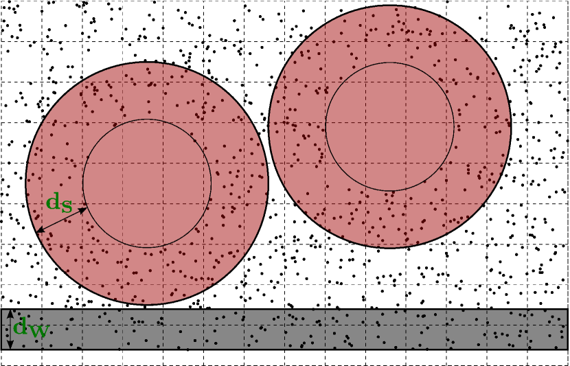
Figure 3: 2D sketch of collision step. Squirmers are shown in red and a wall in grey. Small dots in the white region indicate the fluid particles and dots in the squirmers and in the wall are virtual particles, which are located in a thin layer of thickness $d_{W}=a_{0}$ in the wall and in a thin shell of thickness $d_{S}=\sqrt{3}a_{0}$ in the squirmers. The dashed lines show the collision cell grid.

The virtual particles are placed randomly distributed at density $\rho_{f}$ in a layer of thickness $d_{W}=a_{0}$ inside a bounding wall and in layers of thickness $d_{S}=\sqrt{3}a_{0}$ inside the squirmers, see Fig. 3. It is always guaranteed that grid cells overlapping with walls and squirmers are always completely filled. The positions and velocities of the virtual particles are denoted by $\bar{\mathbf{r}}_{i}$ and $\bar{\mathbf{v}}_{i}$, respectively, with $i=1,\dots,N^{v}$ and $N^{v}$ is the total number of virtual particles. Their velocities are drawn from a normal distribution with the usual standard deviation, $\sigma_{0}=\sqrt{k_{B}T_{0}/m_{0}}$, and zero mean. In addition, virtual particle $i$ located in squirmer $j$ also assumes the local slip velocity of the point $\bar{\mathbf{r}}_{ij}^{\ast}$ on the squirmer surface, which is closest to $\bar{\mathbf{r}}_{i}$, plus the velocity of this point due to the translation and rotation of the squirmer. So, one sets Goetze10

$$\bar{\mathbf{v}}_{i}=\bar{\mathbf{v}}_{i}^{\text{r}}+\mathbf{v}_{s}(\mathbf{e}_{j},\bar{\mathbf{r}}_{ij}^{\ast})+\bm{\Omega}_{j}\times(\bar{\mathbf{r}}_{ij}^{\ast}-\mathbf{R}_{j})+\mathbf{V}_{j},$$ (30)

where $\bar{\mathbf{v}}_{i}^{\text{r}}$ are the random velocities. Then, as usual, fluid and virtual particles are sorted into the cells. We denote the number of fluid and virtual particles in cell $\xi$ by $N_{\xi}^{f}$ and $N_{\xi}^{v}$, respectively. The total number of particles in the cell is $N_{\xi}=N_{\xi}^{f}+N_{\xi}^{v}$. In order to perform now the collision step, the mean velocity in a cell is computed,

$$\mathbf{u}_{\xi}=\frac{1}{N_{\xi}}\left(\sum_{i=1}^{N_{\xi}^{f}}\mathbf{v}_{i}+\sum_{i=1}^{N_{\xi}^{v}}\bar{\mathbf{v}}_{i}\right)\,,$$ (31)

and the new velocities of the particles in a cell are set by the mean velocity $\mathbf{u}_{\xi}$ plus a term given by the collision operator, see Eq. (2).

When the Anderson thermostat is used, random velocities have to be computed, which are denoted by $\mathbf{v}_{i}^{\text{r}}$ and $\bar{\mathbf{v}}_{i}^{\text{r}}$, and which are again drawn from a Gaussian distribution with width $\sigma_{0}=\sqrt{k_{B}T_{0}/m_{0}}$. Then, in order to conserve linear momentum the change of total velocity due to the added random velocities, $\bm{\mathcal{V}}_{\xi}$, has to be subtracted. If conservation of angular momentum is required, by using the collision operator MPC-AT+a, a further term needs to be added. To implement the collision operator, first the center of mass has to be calculated,

$$\mathbf{r}_{\xi}^{s}=\frac{1}{N_{\xi}}\left(\sum_{i=1}^{N_{\xi}^{f}}\mathbf{r}_{i}+\sum_{i=1}^{N_{\xi}^{v}}\bar{\mathbf{r}}_{i}\right),$$ (32)

and the relative positions $\mathbf{r}_{i}^{s}=\mathbf{r}_{i}-\mathbf{r}_{\xi}^{s}$ and $\bar{\mathbf{r}}_{i}^{s}=\bar{\mathbf{r}}_{i}-\mathbf{r}_{\xi}^{s}$. They are needed to calculate the inverse of the moment of inertia tensor $\mathbf{I}^{-1}_{\xi}$ in each cell, where

$$\mathbf{I}_{\xi}=m_{0}\left(\sum_{i=1}^{N_{\xi}^{f}}(|\mathbf{r}_{i}^{s}|^{2}\,\textbf{{1}}-\mathbf{r}_{i}^{s}\otimes\mathbf{r}_{i}^{s})+\sum_{i=1}^{N_{\xi}^{v}}(|\bar{\mathbf{r}}_{i}^{s}|^{2}\,\textbf{{1}}-\bar{\mathbf{r}}_{i}^{s}\otimes\bar{\mathbf{r}}_{i}^{s})\right).$$ (33)

The random velocities added in the collision step change angular momentum by

$$\Delta\bm{\mathcal{L}}_{\xi}=m_{0}\left(\sum_{i=1}^{N_{\xi}^{f}}[\mathbf{r}_{i}^{s}\times(\mathbf{v}_{i}-\mathbf{v}_{i}^{\text{r}})]+\sum_{i=1}^{N_{\xi}^{v}}[\bar{\mathbf{r}}_{i}^{s}\times(\bar{\mathbf{v}}_{i}-\bar{\mathbf{v}}_{i}^{\text{r}})]\right).$$ (34)

To compensate for $\Delta\bm{\mathcal{L}}_{\xi}$ and conserve angular momentum in each cell, the following angular velocity is computed Noguchi07 ,

$$\bm{\omega}_{\xi}^{\text{AMC}}=\mathbf{I}_{\xi}^{-1}\Delta\bm{\mathcal{L}}_{\xi},$$ (35)

and used to rotate the particle velocities in a cell. Thus, by adding the extra terms $\bm{\omega}_{\xi}^{\text{AMC}}\times\mathbf{r}_{i}^{s}$ or $\bm{\omega}_{\xi}^{\text{AMC}}\times\bar{\mathbf{r}}_{i}^{s}$ to the new particle velocities, angular momentum is conserved without changing linear momentum. To summarize, in the collision step the particle velocities are updated according to Noguchi07

$$\begin{split}\mathbf{v}_{i}^{\prime}&=\mathbf{u}_{\xi}+\mathbf{v}_{i}^{\text{r}}-\bm{\mathcal{V}}_{\xi}+\bm{\omega}_{\xi}^{\text{AMC}}\times\mathbf{r}_{i}^{s},\\ \bar{\mathbf{v}}_{i}^{\prime}&=\mathbf{u}_{\xi}+\bar{\mathbf{v}}_{i}^{\text{r}}-\bm{\mathcal{V}}_{\xi}+\bm{\omega}_{\xi}^{\text{AMC}}\times\bar{\mathbf{r}}_{i}^{s}\,.\\ \end{split}$$ (36)

Finally, momentum and angular momentum is transferred to the squirmers, no matter which collision operator has been used. In each collision cell momentum (and angular momentum) is conserved locally but exchanged between fluid particles and virtual particles. The change of momentum for a virtual particle is then

$$\Delta\bar{\mathbf{p}}_{i}=m_{0}(\bar{\mathbf{v}}_{i}^{\prime}-\bar{\mathbf{v}}_{i}).$$ (37)

The momenta and angular momenta of all virtual particles $i$ located in squirmer $j$ are then added up and assigned to squirmer $j$. Thus, after a collision step each squirmer assumes an additional momentum $\Delta\mathbf{P}_{j}^{c}$ and angular momentum $\Delta\mathbf{L}_{j}^{c}$,

$$\begin{split}\Delta\mathbf{P}_{j}^{c}&=\sum_{i=1}^{N_{j}^{v}}\Delta\bar{\mathbf{p}}_{i},\\ \Delta\mathbf{L}_{j}^{c}&=\sum_{i=1}^{N_{j}^{v}}(\bar{\mathbf{r}}_{i}-\mathbf{R}_{j})\times\Delta\bar{\mathbf{p}}_{i},\\ \end{split}$$ (38)

where the sum goes over all virtual particles located in squirmer $j$ with total number $N_{j}^{v}$. So, after each collision step the squirmer velocities and angular velocities are updated according to

$$\begin{split}\mathbf{V}_{j}^{\prime}&=\mathbf{V}_{j}+\frac{1}{M_{S}}\mathbf{P}_{j}^{c},\\ \bm{\Omega}_{j}^{\prime}&=\bm{\Omega}_{j}+\frac{1}{I_{S}}\mathbf{L}_{j}^{c}\,,\end{split}$$ (39)

where $I_{S}$ is the moment of inertia of the squirmer.

5 Dynamics of a squirmer in a narrow slit geometry

Finally, we apply the discussed simulation procedure to the case of a single squirmer moving in a narrow-slit or Hele-Shaw geometry. We use a squirmer of radius $R=3a_{0}$, swimming speed determined by $B_{1}=0.1a_{0}/\tau_{0}$, and choose different values of $\beta=B_{2}/B_{1}$. We place planar walls at positions $x=\pm 4a_{0}$ such that there is only a small gap between squirmer surface and walls. Then, we perform several simulations at various $\beta$ and initial conditions.

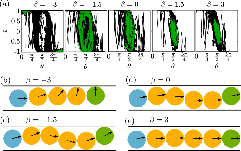
Figure 4: (a) Typical phase portraits from MPCD simulations for a squirmer moving in a narrow-slit geometry. Walls are located at $x=\pm 4a_{0}$ and the radius of the squirmer is $R=3a_{0}$. Thus, minimum and maximum positions of its center are at $x=\pm a_{0}$. The angle $\theta$ indicates the orientation of the squirmer relative to the wall normal. So, $\theta=0$ ($\theta=\pi/2$) is the orientation perpendicular (parallel) to the walls. The long-time dynamics is shown in green. (b-e): Sketch of typical squirmer trajectories for different $\beta$. The initial positions are shown in blue, the final positions in green, and intermediate positions in orange. The orientation vectors are sketched by black arrows.

All the recorded trajectories are shown in Fig. 4(a) where the position $x$ is plotted versus the angle $\theta$, which is the orientation of the squirmer relative to the upper wall normal. For strongly negative $\beta$ values (strong pushers) the squirmer tends to orient perpendicular to the walls (shown for $\beta=-3$ in Fig. 4(a)). This is also sketched in Fig. 4(b). Increasing $\beta$ above a certain value induces oscillations of the swimmer between the walls: The squirmer hits a surface, spends some time there, reorients away from the surface, hits the second surface and so on (shown for $\beta=-1.5$ in Fig. 4(a) and sketched in Fig. 4(c)). A neutral squirmer still performs oscillations but mainly avoids touching the walls by swimming with an orientation performing small oscillations about $\theta=\pi/2$ along the bounding walls, see also Fig. 4(d). In contrast, pullers ($\beta>0$) swim stable between the two walls, as sketched in Fig. 4(e). Interestingly, the $\beta$-dependent dynamics can be captured by considering the lubrication approximation of a squirmer in front of a wall Ishikawa06 ; Schaar2015 , which predicts the correct dynamics for all considered $\beta$ values Zottl2014 .

We also measured the swimming velocity and the flow field around a squirmer with radius $R=3a_{0}$ and surface velocity modes $B_{1}=0.1a_{0}/\tau_{0}$ and $\beta=3$, which swims stable between the plates, by averaging over many realisations and over time. The swimming velocity results in $v_{0}^{\text{MPCD}}=0.0657a_{0}/\tau_{0}$, which is very close to the analytic expression for the swimming speed in bulk $v_{0}=0.0667$ [Eq. (9)]. To obtain the flow fields, the simulation box around the swimmer is divided into small cubic boxes, for which we determine the flow velocity vector. The boxes do not have to coincide with collision cell boxes and may even have higher resolution. Figure 5 shows the flow field (blue arrows) and stream lines (red) for a slice of the field parallel to the walls (top) and perpendicular to the walls (bottom) in the lab fame. Due to the presence of the walls the force dipole fields develop closed loops Cisneros07 ; Hernandez-Ortiz09 . We use a grid size with edge length $a_{0}/2$ to monitor the velocity field, meaning that MPCD is able to resolve flow fields below the the cell size $a_{0}$ of the collision grid.

In Fig. 6 we show the decay of the flow field perpendicular ($v_{\perp}$) and parallel ($v_{||}$) to the swimming direction, which we compare to the decay in bulk using the analytic expressions [Eq. (13)]. Due to the leading force dipole field, they decay with $\sim r^{-2}$. For intermediate distances away from the squirmer the flow fields obtained from our simulations in strong confinement show a similar decay. Indeed it has been shown analytically that for very strong confinement flow fields of microswimmers decay in general with $\sim r^{-2}$ Brotto2013 ; Blaschke2016 . However, in our simulations the decay of the flow fields far away from the squirmer is faster, which probably stems from the periodic boundary conditions Hu2015 ; Zottl2017 . Also, the fact that the strength of the flow field in front of the swimmer is weaker than at the back may be a signature of the periodic boundary conditions or due to the fact that MPCD does not model a perfect incompressible Stokes flow, but finite Reynolds and Schmidt numbers which account for finite fluid inertia and compressibility, respectively Padding06 ; Gompper08 .

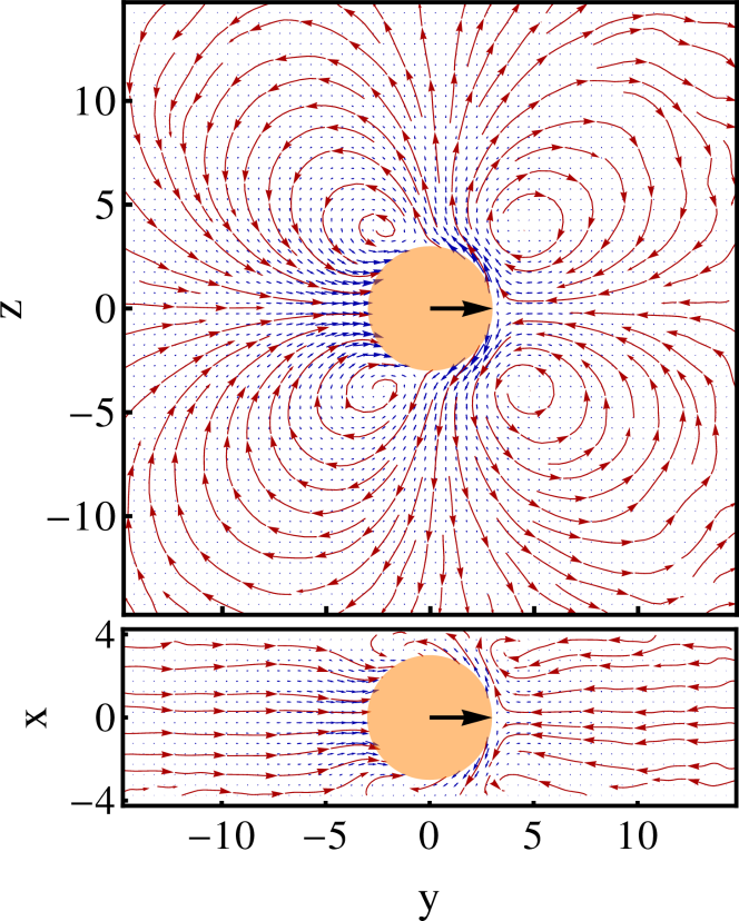
Figure 5: Flow field for a puller swimming in a narrow-slit geometry. The velocity field is indicated in blue and streamlines in red. Top: Top view of the flow field. Bottom: side view.

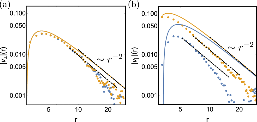
Figure 6: (a) Decay of the flow field perpendicular ($v_{\perp}$) to the swimmer direction. The flow field in the $-z$ direction is shown in blue, and in the $+z$ direction in orange. (b) Decay of the flow field parallel ($v_{||}$) to the swimmer direction. The flow field in the $+y$ direction (front of the swimmer) is shown in blue, and in the $-y$ direction (back of the swimmer) in orange. Solid lines are curves obtained from the analytic model of a squirmer in bulk [Eq. (13)].

6 Conclusion

Here we have reviewed and discussed how simple spherical model swimmers – squirmers – can be modeled and simulated using the method of multiparticle collision dynamics. We have shown how the dynamics of the fluid and the squirmers is coupled both in the streaming step and in the collision step, where a correct momentum and angular momentum transfer between particles ensures correct hydrodynamics Downton09 and thermal fluctuations Goetze10 . In order to enhance the accuracy of the flow fields around the squirmer, the use of virtual particles inside squirmers, which contribute to the collision step, is necessary. Also bounding surfaces and pressure-driven flows can be simulated straightforward. Since the method models the fluid explicitely via effective fluid particles, thermal noise is included naturally in the simulation. In order to obtain smooth flow fields averaging over several realisations and over time is necessary.

References

- (1) A. Zöttl and H. Stark, J. Phys.: Condens. Matter 28, 253001 (2016).
- (2) C. Bechinger, R. Di Leonardo, H. Löwen, C. Reichhardt, G. Volpe, and G. Volpe, Rev. Mod. Phys. 88, 045006 (2016).
- (3) C. C. Maass, C. Krüger, S. Herminghaus, and C. Bahr, Annu. Rev. Condens. Matter Phys. 7, 171 (2016).
- (4) G. I. Taylor, Proc. R. Soc. A 209, 447 (1951).
- (5) J. Lighthill, Commun. Pure Appl. Math. 5, 109 (1952).
- (6) J. R. Blake, J. Fluid Mech. 46, 199 (1971).
- (7) A. Najafi and R. Golestanian, Phys. Rev. E 69, 062901 (2004).
- (8) J. E. Avron, O. Kenneth, and D. H. Oaknin, New J. Phys. 7, 234 (2005).
- (9) J. L. Münch, D. Alizadehrad, S. B. Babu, and H. Stark, Soft Matter 12, 7350 (2016).
- (10) G. Rückner and R. Kapral, Phys. Rev. lett. 98, 150603 (2007).
- (11) Y. G. Tao and R. Kapral, J. Chem. Phys. 128, 164518 (2008).
- (12) Y. G. Tao and R. Kapral, J. Chem. Phys. 131, 024113 (2009).
- (13) Y.-G. Tao and R. Kapral, ChemPhysChem 10, 770 (2009).
- (14) S. Thakur and R. Kapral, J. Chem. Phys. 133, 204505 (2010).
- (15) S. Thakur and R. Kapral, Soft Matter 6, 756 (2010).
- (16) S. Thakur and R. Kapral, J. Chem. Phys. 135, 024509 (2011).
- (17) S. Thakur, J. X. Chen, and R. Kapral, Angew. Chem. Int. Ed. 50, 10165 (2011).
- (18) M. Yang and M. Ripoll, Phys. Rev. E 84, 061401 (2011).
- (19) S. Thakur and R. Kapral, Phys. Rev. E 85, 026121 (2012).
- (20) M.-J. Huang, H.-Y. Chen, and A. S. Mikhailov, Eur. Phys. J. E 35, 119 (2012).
- (21) P. de Buyl and R. Kapral, Nanoscale, 5, 1337 (2013).
- (22) R. Kapral, J. Chem. Phys. 138, 020901 (2013).
- (23) M. Yang and M. Ripoll, Soft Matter 9, 4661 (2013).
- (24) M. Yang, A. Wysocki and M. Ripoll, Soft Matter 10, 6208 (2014).
- (25) M. Wagner and M. Ripoll, Eur. Phys. Lett. 119 66007 (2017).
- (26) Y. Yang, F. Qiu, and G. Gompper, Phys. Rev. E 89, 012720 (2014).
- (27) Y. Yang, J. Elgeti, and G. Gompper, Phys. Rev. E 78, 061903 (2008).
- (28) J. Elgeti and G. Gompper, NIC Symp. 39, 53 (2008).
- (29) J. Elgeti and G. Gompper, Eur. Phys. Lett. 85, 38002 (2009).
- (30) J. Elgeti, U. B. Kaupp, and G. Gompper, Biophys. J 99, 1018 (2010).
- (31) Y. Yang, V. Marceau, and G. Gompper, Phys,. Rev. E 82, 031904 (2010).
- (32) S. Y. Reigh, R. G. Winkler, and G. Gompper, Soft Matter 8, 4363 (2012).
- (33) S. Y. Reigh, R. G. Winkler, and G. Gompper, PLoS ONE 8, e70868 (2013).
- (34) J. Elgeti and G. Gompper, Proc. Natl. Am. Sci. U.S.A. 110, 4470 (2013).
- (35) Y. Yang, F. Qiu, and G. Gompper, Phys. Rev. E 89, 012720 (2014).
- (36) A. Agrawal and S. B. Babu, Phys. Rev. E 97, 020401(R) (2018).
- (37) F. J. Schwarzendahl and M. G. Mazza, arXiv:1711.08689 (2017).
- (38) J. Hu, M. Yang, G. Gompper, and R. G. Winkler, Soft Matter 11, 7867 (2015).
- (39) J. Hu, A. Wysocki, G. Gompper, and R. G. Winkler, Sci. Rep. 5, 9586 (2015).
- (40) A. Zöttl and J. M. Yeomans, arXiv:1710.03505 (2017).
- (41) S. B. Babu and H. Stark, New J. Phys. 14, 085012 (2012).
- (42) N. Heddergott, T. Krüger, S. B. Babu, A. Wei, E. Stellamanns, S. Uppaluri, T. Pfohl, H. Stark, and M. Engstler, PLoS Pathog. 8(11), e1003023 (2012).
- (43) D. Alizadehrad, Tim Krüger, M. Engstler, and H. Stark, PLoS Comput. Biol. 11, e1003967 (2015).
- (44) T. Eisenstecken, J. Hu, and R. G. Winkler, Soft Matter 12, 8316 (2016).
- (45) M. T. Downton and H. Stark, J. Phys. Condens. Matt. 21, 204101 (2009).
- (46) I. O. Götze and G. Gompper, Phys. Rev. E 82, 041921 (2010).
- (47) A. Zöttl and H. Stark, Phys. Rev. Lett. 108, 218104 (2012).
- (48) A. Zöttl and H. Stark, Phys. Rev. Lett. 112, 118101 (2014).
- (49) K. Schaar, A. Zöttl, and H. Stark, Phys. Rev. Lett. 115, 038101 (2015).
- (50) J. Blaschke, M. Maurer, K. Menon, A. Zöttl, and H. Stark, Soft Matter 12, 9821 (2016).
- (51) M. Theers, E. Westphal, G. Gompper, and R. G. Winkler, Soft Matter 12, 7372 (2016).
- (52) J.-T. Kuhr, J. Blaschke, F. Rühle, and H. Stark, Soft Matter 13, 7548 (2017).
- (53) F. Rühle, J. Blaschke, J.-T. Kuhr, and H. Stark, New J. Phys. 20, 025003 (2018).
- (54) R. Kapral, Adv. Chem. Phys. 140, 89 (2008).
- (55) G. Gompper, T. Ihle, D. M. Kroll, and R. G. Winkler, Adv. Polym. Sci. 221, 1 (2008).
- (56) A. Malevanets and R. Kapral, J. Chem. Phys. 110, 8605 (1999).
- (57) A. Malevanets and R. Kapral, J. Chem. Phys. 112, 7260 (2000).
- (58) T. Ihle and D. M. Kroll, Phys. Rev. E 63, 066705 (2003); 63, 066706 (2003).
- (59) T. Ihle and D. M. Kroll, Phys. Rev. E 63, 020201 (2001).
- (60) E. Tüzel, M. Strauss, T. Ihle, and D. M. Kroll, Phys. Rev. E 68, 036701 (2003).
- (61) C. M. Pooley and J. M. Yeomans, J. Phys. Chem. B 109, 6505 (2005).
- (62) E. Tüzel, T. Ihle, and D. M. Kroll, Phys. Rev. E 74, 056702 (2006).
- (63) H. Noguchi, N. Kikuchi, and G. Gompper, Europhys. Lett. 78, 10005 (2007).
- (64) H. Noguchi and G. Gompper, Phys. Rev. E 78, 016706 (2008).
- (65) I. O. Götze, H. Noguchi, and G. Gompper, Phys. Rev. E 76, 046705 (2007).
- (66) C. Brennen and H. Winet, Annu. Rev. Fluid Mech. 9, 339 (1977).
- (67) S. Kim and S. Karila, Microhydrodynamics, (Butterworth-Heinemann, Newton, MA, 1991).
- (68) J. Happel and H. Brenner, Low Reynolds Number Hydrodynamics: with special applications to particulate media, (Springer, New York, 1983).
- (69) M. Schmitt and H. Stark, Eur. Phys. Lett. 101, 44008 (2013).
- (70) M. Schmitt and H. Stark, Eur. Phys. J. E 39, 80 (2016).
- (71) T. Ishikawa and M. Hota, J. Exp. Biol. 209, 4452 (2006).
- (72) T. J. Pedley, D. R. Brumley, and R. E. Goldstein, J. Fluid Mech. 798, 165 (2016).
- (73) T. Ishikawa, M. P. Simmonds, and T. J. Pedley, J. Fluid Mech. 568, 119 (2006).
- (74) J. L. Anderson, Ann. Rev. Fluid Mech. 21, 61 (1989).
- (75) H. A. Stone and A. D. T. Samuel, Phys. Rev. Lett. 77, 4102 (1996).
- (76) S. Thutupalli, R. Seemann, and S. Herminghaus, New J. Phys. 13, 073021 (2011).
- (77) V. Magar, T. Goto, and T. J. Pedley, Q. J. Mech. Appl. Math. 56, 65 (2003).
- (78) V. Magar and T. J. Pedley, J. Fluid Mech. 539, 93 (2005).
- (79) D. Giacché, T. Ishikawa, and T. Yamaguchi, Phys. Rev. E 82, 056309 (2010).
- (80) T. Ishikawa and T. J. Pedley, J. Fluid. Mech 588, 437-462 (2007).
- (81) T. Ishikawa, T. J. Pedley, and T. Yamaguchi, J. Theor. Biol. 249, 296-306 (2007).
- (82) T. Ishikawa, J. T. Locsei, and T. J. Pedley, J. Fluid Mech. 615, 401 (2008).
- (83) T. Ishikawa, J. T. Locsei, and T. J. Pedley, Phys. Rev. E 82, 021408 (2010).
- (84) A. A. Evans, T. Ishikawa, T. Yamaguchi, and E. Lauga, Phys. Fluids 23, 111702 (2011).
- (85) T. Ishikawa and T. J. Pedley, J. Fluid. Mech 588, 399 (2007).
- (86) T. Ishikawa, J. Fluid. Mech. 705, 98 (2012).
- (87) I. Pagonabarraga and I. Llopis, Soft Matter 9, 7174 (2013).
- (88) T. Ishikawa and T. J. Pedley, Phys. Rev. Lett. 100, 088103 (2008).
- (89) S. Michelin and E. Lauga, Phys. Fluids 22, 111901 (2010).
- (90) S. Michelin and E. Lauga, Phys. Fluids 23, 101901 (2011).
- (91) S. Wang and A. M. Ardekani, Phys. Fluids 24, 101902 (2012).
- (92) A. S. Khair and N. G. Chisholm, Phys. Fluids 26, 011902 (2014).
- (93) N. G. Chisholm, D. Legendre, E. Lauga, and A. S. Khair, J. Fluid. Mech. 796, 233 (2016).
- (94) G. Li, A. Ostace, and A. M. Ardekani, Phys. Rev. E 94, 053104 (2016).
- (95) S. Wang and A. M. Ardekani, J. Fluid Mech. 702, 286 (2012).
- (96) A. Doostmohammadi, R. Stocker, and A. M. Ardekani, Proc. Natl. Am. Sci. U.S.A. 109, 3856 (2012).
- (97) K. Ishimoto, J. Fluid Mech. 723, 163 (2013).
- (98) A. M. Leshansky, Phys. Rev. E 80, 051911 (2009).
- (99) L. Zhu, M. Do-Quang, E. Lauga, and L. Brandt, Phys. Rev. E 83, 011901 (2011).
- (100) L. Zhu, E. Lauga, and L. Brandt, Phys. Fluids 24, 051902 (2012).
- (101) C. Datt, L. Zhu, G. J. Elfring, and O. S. Pak, J. Fluid. Mech. 784, R1 (2015).
- (102) M. De Corato, F. Greco, and P. L. Maffettone, Phys. Rev. E 92, 053008 (2015).
- (103) H. Nganguia, K. Pietrzyk, and O. S. Pak, Phys. Rev. E 96, 062606 (2017).
- (104) Z. Lin, J. Thiffeault, and S. Childress, J. Fluid Mech. 669, 167 (2011).
- (105) D. Pushkin, H. Shum, and J. M. Yeomans, J. Fluid Mech. 726, 5 (2013).
- (106) N. Aguillon, A. Decoene, B. Fabréges, B. Maury, and B. Semin, ESAIM: Proc. 38, 36 (2012).
- (107) J. J. Molina, Y. Nakayama, and R. Yamamoto, Soft Matter 9, 4923 (2013).
- (108) F. Alarcon and I. Pagonabarraga, J. Mol. Liq. 185, 56 (2013).
- (109) R. Matas-Navarro, R. Golestanian, T. B. Liverpool, and S. M. Fielding, Phys. Rev. E 90, 032304 (2014).
- (110) K. Kyoya, D. Matsunaga, Y. Imai, T. Omori, and T. Ishikawa, Phys. Rev. E 92, 063027 (2015).
- (111) N. Oyama, J. J. Molina, and R. Yamamoto, Phys. Rev. E 93, 043114 (2016).
- (112) J.-B. Delfau, J. J. Molina, and M. Sano, Europhys. Lett. 114, 24001 (2016).
- (113) N. Yoshinaga and T. B. Liverpool, Phys. Rev. E 96, 020603(R) (2017).
- (114) F. Alarcon, C. Valeriani I. Pagonabarraga Soft Matter 13, 814 (2017).
- (115) A. Chamolly, T. Ishikawa, and E. Lauga, New J. Phys. 19 115001 (2017).
- (116) J. S. Lintuvuori, A. Würger, and K. Stratford, Phys. Rev. Lett. 119, 068001 (2016).
- (117) I. Llopis and I. Pagonabarraga, J. Non-Newtonian. Fluid Mech. 165, 946 (2010).
- (118) S. E. Spagnolie and E. Lauga, J. Fluid Mech. 700, 105 (2012).
- (119) S. Wang and A. M. Ardekani, Phys. Rev. E 87, 063010 (2013).
- (120) L. Zhu, E. Lauga, and L. Brandt, J. Fluid. Mech. 726, 285 (2013).
- (121) K. Ishimoto and E. A. Gaffney, Phys. Rev. E 88, 062702 (2016).
- (122) G.-J. Li and A. M. Ardekani, Phys. Rev. E 90, 013010 (2014).
- (123) D. Papavassiliou and G. P. Alexander, Europhys. Lett. 110, 44001 (2015).
- (124) J. S. Lintuvuori, A. T. Brown, K. Stratford, and D. Marenduzzo, Soft Matter 12, 7959 (2016).
- (125) J. Simmchen, J. Katuri, W. E. Uspal, M. N. Popescu, M. Tasinkevych, and S. Sanchez, Nat. Comm. 7, 10598 (2016).
- (126) Z. Shen, A. Würger, and J. S. Lintuvuori, arXiv:1711.09699 (2017).
- (127) R. Matas Navarro and I. Pagonabarraga, Eur. Phys. J. E 33, 27 (2010).
- (128) J. T. Padding and A. A. Louis, Phys. Rev. E 74, 031402 (2006).
- (129) J. D. Weeks, D. Chandler, and H. C. Anderson, J. Chem. Phys. 54, 5237 (1971).
- (130) L. Verlet, Phys. Rev. Z 159, 98 (1967).
- (131) W. C. Swope, H. C. Andersen, P. H. Berens, and K. R. Wilson, J. Chem. Phys. 76, 637 (1982).
- (132) M. P. Allen and D. J. Tildesley, Computer simulation of liquids, (Clarendon Press, Oxford, 1987).
- (133) E. Allahyarov and G. Gompper, Phys. Rev. E 66, 036702 (2002).
- (134) J. T. Padding, A. Wysocki, H. Löwen, and A. A. Louis, J. Phys.: Condens. Matter 17, S3393 (2005).
- (135) A. Lamura, G. Gompper, T. Ihle, and D. M. Kroll, Europhys. Lett. 56, 319 (2001).
- (136) L. H. Cisneros, R. Cortez, C. Dombrowski, R. E. Goldstein, and J. Kessler, Exp. Fluids 43, 737, (2007).
- (137) J. P. Hernandez-Ortiz, P. T. Underhill, and M. D. Graham, J. Phys.: Condens. Matter 21, 204107 (2009).
- (138) T. Brotto, J.-B. Caussin, E. Lauga, and D. Bartolo, Phys. Rev. Lett. 110, 038101 (2013).