The structure of ultrafine entanglement witnesses

Abstract

An entanglement witness is an observable with the property that a negative expectation value signals the presence of entanglement. The question arises how a witness can be improved if the expectation value of a second observable is known, and methods for doing this have recently been discussed as so-called ultrafine entanglement witnesses. We present several results on the characterization of entanglement given the expectation values of two observables. First, we explain that this problem can naturally be tackled with the method of the Legendre transformation, leading even to a quantification of entanglement. Second, we present necessary and sufficient conditions that two product observables are able to detect entanglement. Finally, we explain some fallacies in the original construction of ultrafine entanglement witnesses [F. Shahandeh et al., Phys. Rev. Lett. 118, 110502 (2017)].

1 Introduction

Entanglement is a central phenomenon in quantum information processing and entanglement witnesses provide some of the most effective tools for detecting it [1, 2]. Mathematically, an entanglement witness is a Hermitean operator $W$, such that $\operatorname{Tr}(\sigma W)\geq 0$ holds for every separable state $\sigma\in\mathcal{S}_{\rm sep}$. Consequently, measuring a negative expectation value $\operatorname{Tr}(\varrho W)<0$ implies that the state $\varrho$ is entangled.

Any entanglement witness can be written as

$$W=g_{s}\mathbbm{1}-L,$$ (1)

where $L$ is the observable actually to be measured in an experiment and $g_{s}$ characterizes the relation of $L$ to separability. It is defined as the maximal value that $L$ can attain on separable states, $g_{s}=\sup_{\sigma}\{\operatorname{Tr}(\sigma L)|\sigma\in\mathcal{S}_{\rm sep}\}$. The physical interpretation of the witness is then clear: If one measures an expectation value $l={\langle{L}\rangle}$ larger than $g_{s}$, the state must be entangled and ${\langle{W}\rangle}<0$.

Some remarks are in order. First, since the set of separable states is defined as the convex hull of all pure product states, the state $\sigma_{\rm opt}$ where the expression $\{\operatorname{Tr}(\sigma L)|\sigma\in\mathcal{S}_{\rm sep}\}$ is maximal is a pure product state, which simplifies the computation of $g_{s}.$ Second, for many possible $L$, the computation of $g_{s}$ can be carried out analytically, for instance if $L=|\psi\rangle\!\langle\psi|$ is a projector onto a pure state [2]. Finally, it can happen, of course, that the observable $L$ is not useful for entanglement detection at all. This is the case, if the maximal eigenvalue of $L$ coincides with $g_{s}$ and consequently no state can have an expectation value ${\langle{L}\rangle}$ that exceeds the maximal value for separable states.

What changes, if in addition to $l={\langle{L}\rangle}$ the expectation value $c={\langle{C}\rangle}$ of a second observable $C$ is known? From the knowledge of the two observables, one can determine the expectation value of $X=\alpha C+\beta L$ for any values of $\alpha,\beta.$ Consequently, any witness of the type

$$W(\alpha,\beta)=g_{s}(\alpha,\beta)\mathbbm{1}-X$$ (2)

can be evaluated. From the convexity of the set of separable states it also follows that any state whose entanglement can be proved from the knowledge of $l={\langle{L}\rangle}$ and $c={\langle{C}\rangle}$ must be detected by the witness from Eq. (2) for some $\alpha,\beta$.

A different approach, called ultrafine entanglement witnessing (UEW) was recently introduced [3, 4] and further developed [5]. Here, one starts from Eq. (1) and asks how $g_{s}$ can be changed due to the knowledge of $c={\langle{C}\rangle}$. In fact, one can then define

$$g_{s}=\sup_{\sigma}\{\operatorname{Tr}(\sigma L)|\sigma\in\mathcal{S}_{\rm sep}\mbox{ and }\operatorname{Tr}(\sigma C)=c\}.$$ (3)

Of course, evaluating this is more complicated, and the question arises how one can characterize the optimal $\sigma_{\rm opt;c}$ which is the separable state obeying ${\rm Tr}(C\sigma_{\rm opt;c})=c$ and maximizing the expectation value of $L$.

A second question is, whether one can derive conditions on $L$ and $C$ which guarantee that the knowledge of ${\rm Tr}(\varrho{C})$ improves the capability of $L$ to detect entanglement. In an experimental setting, one typically considers observables which are easy to implement, so one may take $L=L_{A}\otimes L_{B}$ and $C=C_{A}\otimes C_{B}$ to be product observables. In this case, $l={\langle{L}\rangle}$ (or $c={\langle{C}\rangle}$) alone is clearly not sufficient to detect entanglement, so the question arises what conditions $C$ and $L$ have to fulfill in order to detect entanglement together. So far, a conjecture has been presented [3], but its rigorous derivation remained elusive.

In this paper, we present several results on the characterization of entanglement from the expectation values of two observables. In Section II we start with the problem in Eq. (2). We explain how the problem can be solved using the method of the Legendre transformation. We stress that this approach is not new [6, 7], but we present an analytical example useful for our later discussion. In Section III we study the question, which conditions $L=L_{A}\otimes L_{B}$ and $C=C_{A}\otimes C_{B}$ have to fulfill in order to be able to detect entanglement. We solve the problem for two qubits and present extensions, as well as interesting counterexamples, for higher dimensions. In Section IV we critically discuss the results of Ref. [3] in some detail. Some errors in this reference have been already corrected in an erratum [4], but it is instructive to study precisely the fallacies. Finally, we conclude and discuss some open problems for further research.

2 Legendre transformation

In this section, we consider the general task of characterizing entanglement from two known expectation values. More precisely, given the two expectation values $c=\operatorname{Tr}{(\varrho C)}$ and $l=\operatorname{Tr}{(\varrho L)}$ of the observables $C$ and $L$, we want to find a lower bound on the value of some entanglement measure $E(\varrho)$ of the state $\varrho$. The method we explain uses the Legendre transformation. It is not new and has been introduced in Refs. [6, 7].

The connection to UEW introduced in Ref. [3] is simple: The method of Legendre transformations gives a non-trivial bound on some faithful entanglement measure for the states compatible with $c$ and $l$, if and only if these observables are useful for UEW. UEWs, however, can only certify entanglement, while the method of Legendre transformation provides a systematic way to estimate entanglement quantitatively. In addition, the Legendre transformation treats the observables $C$ and $L$ in a symmetric manner.

2.1 The general method

We need to compute the minimal value of $E(\varrho)$ over all states compatible with the observed data,

$$\varepsilon(c,l)=\inf_{\varrho}\{E(\varrho)\,|\,\operatorname{Tr}{(\varrho C)}=c\mbox{ and }\operatorname{Tr}{(\varrho L)}=l\}.$$ (4)

If the entanglement measure $E(\varrho)$ is convex, then this is a convex function in $c$ and $l$. As such, it can be characterized as the supremum over all affine functions below it. Therefore, given $c$ and $l$, we would like to find the smallest constant $k\in\mathbb{R}$, such that

$$\varepsilon(c,l)\geq\alpha c+\beta l-k$$ (5)

for arbitrary $\alpha$ and $\beta\in\mathbb{R}$. Rewriting Eq. (5), we obtain

$$k:=\hat{E}(X)= \sup_{c,l}\{\alpha c+\beta l-\varepsilon(c,l)\}$$

$$= \sup_{\varrho}\{\alpha\operatorname{Tr}{(\varrho C)}+\beta\operatorname{Tr}{(\varrho L)}-E(\varrho)\},$$ (6)

which is the definition of $\hat{E}$ as the Legendre transform of the entanglement measure $E$, evaluated for the operator

$$X=\alpha C+\beta L.$$ (7)

The value of $k$ can in turn be used to obtain the supremum over all slopes $\alpha$ and $\beta$:

$$\varepsilon(c,l)=\sup_{\alpha,\beta}\{\alpha c+\beta l-\hat{E}(X)\}.$$ (8)

This is itself a Legendre transform of $\hat{E}(X)$ and gives a lower bound on the entanglement measure $E(\varrho)$ from the values $c$ and $l$. It follows from convex geometry that this lower bound is optimal, in the sense that there is one state with the values $c$ and $l$ having the entanglement $E(\varrho)=\varepsilon(c,l)$. Also, it should be noted that there is a practical difference between Eq. (6) and Eq. (8): For obtaining a valid lower bound on $E(\varrho)$ one needs the global optimum in the maximization in Eq. (6). In Eq. (8), however, any pair of values $\alpha,\beta$ gives already a valid lower bound.

2.2 A concrete example

Whether one can analytically evaluate Eqs. (6, 8) depends on the entanglement measure $E$ and the specific form of $C$ and $L$. For measures that are defined via the convex roof construction,

$$E(\varrho)=\inf_{p_{i},|\psi_{i}\rangle}\sum_{i}p_{i}E(|\psi_{i}\rangle),$$ (9)

with $\varrho=\sum_{i}p_{i}|\psi_{i}\rangle\!\langle\psi_{i}|$, the Legendre transform can be evaluated by optimizing over pure states only [6]:

$$E(X)=\sup_{|\psi\rangle}\{\langle\psi|X|\psi\rangle-E(|\psi\rangle)\}.$$ (10)

Here, we concentrate on the geometric measure of entanglement $E_{G}$ [8] defined for pure states as one minus the maximal overlap with product states,

$$E_{G}(|\psi\rangle)=1-\sup_{|\phi\rangle=|a\rangle|b\rangle|c\rangle\dots}\left|\left\langle\phi|\psi\right\rangle\right|^{2},$$ (11)

and for mixed states via a convex roof construction. Thus, we need to evaluate

$$E_{G}(X)=\sup_{|\psi\rangle}\sup_{|\phi\rangle=|a\rangle|b\rangle|c\rangle\dots}\{\langle\psi|(X+|\phi\rangle\!\langle\phi|)|\psi\rangle-1\}.$$ (12)

This optimization can be done in practice numerically in an efficient manner [6]. Here, however, we consider a specific case of $X$ where analytical derivations can be made. We choose

$$C=\sigma_{z}\otimes\sigma_{z},\quad L=\sigma_{x}\otimes\sigma_{x}.$$ (13)

The operator $X$ accordingly is then diagonal in the Bell basis with eigenvalues $(\alpha+\beta,\alpha-\beta,-\alpha+\beta,-\alpha-\beta)$. For such operators, the Legendre transformation of the geometric measure is given by [9]

$$E_{G}(X)=\frac{\lambda_{1}+\lambda_{2}-1}{2}+\frac{1}{2}\sqrt{(\lambda_{1}-\lambda_{2})^{2}+1},$$ (14)

where $\lambda_{1}$ denotes the largest, and $\lambda_{2}$ denotes the second-largest eigenvalue of X.

For $c=\operatorname{Tr}{(\varrho C)}$ and $l=\operatorname{Tr}{(\varrho L)}$ we can assume without loss of generality that $c\geq l\geq 0$, as this can be achieved for the given observables by local unitary transformations that do not alter the entanglement. In addition, we have $c\leq 1$. It is easy to see that the higher the values of $c$ and $l$, the more entangled the state is. From this it follows that in Eq. (8) the interesting case is if $\alpha$ and $\beta$ both have positive values.

We have to distinguish between two cases, $\alpha\geq\beta\geq 0$ and $\beta\geq\alpha\geq 0$. First, assume that $\alpha\geq\beta\geq 0$, then

$$\varepsilon(c,l)= \sup_{\alpha,\beta}\bigg{[}\alpha(l-1)+\frac{1}{2}+\beta c-\sqrt{\beta^{2}+\frac{1}{4}}\bigg{]}.$$ (15)

Taking the partial derivative with respect to $\alpha$ we obtain $\partial_{\alpha}\varepsilon(c,l)=(l-1)\leq 0$, therefore $\alpha$ must be chosen as small as possible, i.e., $\alpha=\beta$. Inserting this and taking the partial derivative with respect to $\beta$ we find

$$\partial_{\beta}\varepsilon(c,l)=(c+l-1)-\frac{\beta}{\sqrt{\beta^{2}+\frac{1}{4}}}\overset{!}{=}0,$$ (16)

and consequently $\beta={(c+l-1)}/{[2\sqrt{1-(c+l-1)^{2}}]}$. This yields the final result:

$$E_{G}\geq\varepsilon(c,l)=\frac{1}{2}\left(1-\sqrt{1-(c+l-1)^{2}}\right).$$ (17)

Considering the second case, $\beta\geq\alpha\geq 0$, the second largest eigenvalue changes from $\alpha-\beta$ to $\beta-\alpha$. The function to maximize is essentially the same as before, but with $\alpha$ and $\beta$ swapped. Therefore, the solution is the same and Eq. (17) also holds. The corresponding bounds on the geometric measure are depicted in Fig. 1.

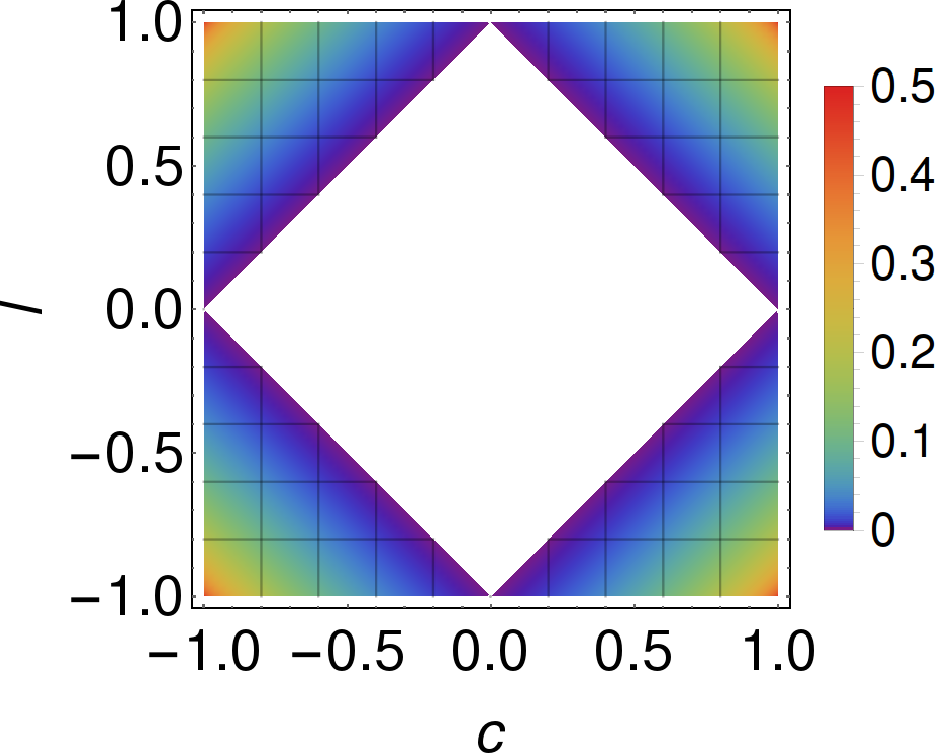
Figure 1: Lower bounds on the geometric measure of entanglement based on the expectation values $c=\operatorname{Tr}(\varrho\sigma_{z}\otimes\sigma_{z})$ and $l=\operatorname{Tr}(\varrho\sigma_{x}\otimes\sigma_{x})$. The white inner region corresponds to separable states.

2.3 Necessary and sufficient criterion for two qubits

In this case, we can directly formulate the main result:

Proposition 1. Consider a two-qubit system and product operators $C=C_{A}\otimes C_{B}$ and $L=L_{A}\otimes L_{B}$. $C$ and $L$ can be used for entanglement detection, if and only if $[C_{A},L_{A}]\neq 0$ and $[C_{B},L_{B}]\neq 0$.

Proof. One direction is trivial and valid for any dimension: If $[C_{A},L_{A}]=0$, then $C$ and $L$ cannot be used for entanglement detection. The reason is that in this case Alice is effectively performing only a single measurement $M_{A}$. So, any possible linear combination $X=\alpha C+\beta L$ can be evaluated from the statistics of a product measurement $M_{A}\otimes M_{B}$, (where $M_{B}$ may depend on $\alpha,\beta$) and for such measurements the probabilities can always be mimicked by a separable state. A similar reasoning holds if $[C_{B},L_{B}]=0.$

For the other direction we need to prove that for some real valued $\alpha$ and $\beta$ the operator

$$X=\alpha C+\beta L$$ (18)

has an entangled ground (lowest eigenvalue) state. This ground state can then be certified by the appropriate combination of $C$ and $L$, thus its entanglement can be detected.

Let us consider $\alpha=1$ and $\beta=\lambda$, where $\lambda$ is a very small real number. We can assume that the operators $C_{A}$ and $C_{B}$ are diagonal in their respective local computational basis, so $C$ is diagonal in $|kl\rangle$, $k,l\in\{0,1\}$ with eigenvalues $\gamma_{kl}$. We need to distinguish two cases, depending on whether the operator $C$ has a degenerate ground state or not.

First case: Let us assume that $C$ has the unique ground state $|00\rangle$. Considering $\lambda L$ as a perturbation to $C$, the first order correction to the ground state is given by [10]

$$|\psi_{1}\rangle=\sum_{k\neq 0,l\neq 0}\frac{\langle kl|L|00\rangle}{\gamma_{00}-\gamma_{kl}}|kl\rangle.$$ (19)

We now prove the statement by contradiction, i.e. we assume that the ground state of the operator $C+\lambda L$ is always a product state. For small values of $\lambda$, the ground state can, according to perturbation theory, be expanded as

$$|\psi(\lambda)\rangle=|00\rangle+\lambda|\psi_{1}\rangle+\lambda^{2}|\psi_{2}\rangle+\dots.$$ (20)

As the total state is normalized, $|\psi_{1}\rangle$ is orthogonal to $|00\rangle$.

The first observation is that from the fact that $|\psi(\lambda)\rangle$ is a product state, it follows that $|\psi_{1}\rangle$ must also be orthogonal to all $|kl\rangle$, where $k,l>0$. For qubits, this only concerns the case $k=l=1$, but we formulate the argument directly for arbitrary dimensions. This orthogonality can be seen as follows: Assume that $0<f:=\langle kl|\psi_{1}\rangle$ for $k,l>0$, and consider the state $|\varphi\rangle=(|00\rangle+|kl\rangle)/{\sqrt{2}}$. The state $|\varphi\rangle$ is entangled and it is known that for every product state $|a,b\rangle$ one has $|\langle a,b|\varphi\rangle|^{2}\leq 1/2$ [2]. For $\lambda=0$, we have that $|\langle\psi(0)|\varphi\rangle|^{2}=1/2$ and in addition

$$\frac{\partial}{\partial\lambda}|\langle\psi(\lambda)|\varphi\rangle|\big{|}_{\lambda=0}=f>0,$$ (21)

so for small $\lambda$ the overlap obeys $|\langle\psi(\lambda)|\varphi\rangle|^{2}>1/2$. Consequently $|\psi(\lambda)\rangle$ is entangled and we arrive at a contradiction.

Having established that $|kl\rangle$ for $k,l>0$ is orthogonal to the first order expansion vector $|\psi_{1}\rangle$ we can conclude from Eq. (19) that

$$\langle 11|L|00\rangle=\langle 00|L|11\rangle=0.$$ (22)

Since $L=L_{A}\otimes L_{B}$, it follows that either $L_{A}$ or $L_{B}$ must be diagonal in the computational basis. This is the contradiction to the statement that $[C_{x},L_{x}]\neq 0$ for $x\in\{A,B\}$.

Second case: Now we consider the case when $C$ is degenerate, in which case both the ground (lowest eigenvalue) state and the most excited (highest eigenvalue) state must have two-fold degeneracy. This is because if only the ground state would be degenerate, the operator $-C$ could be used instead and the first case of the proof would apply.

Since we have the assumption that neither $C_{A}$ or $C_{B}$ commutes with $L_{A}$ or $L_{B}$, respectively, neither $C_{A}$ not $C_{B}$ can be proportional to the identity. It follows that without loss of generality we can fix the degenerate ground subspace to be spanned by the two product vectors $|00\rangle$ and $|11\rangle$. Note that in this two-dimensional subspace, $|00\rangle$ and $|11\rangle$ are the only product vectors.

The operator $C$ is disturbed by the operator $L$ and we want to characterize this using degenerate perturbation theory [10]. We define the projector $P=|00\rangle\!\langle 00|+|11\rangle\!\langle 11|$ and, according to perturbation theory, we need to diagonalize the operator $PLP$. The ground state $|\chi\rangle$ of this operator is then the zeroth order of perturbation theory, that is in the limes $\lambda\searrow 0$ the ground state of the perturbed system approximates $|\chi\rangle$ arbitrarily well.

The vectors $|00\rangle$ and $|11\rangle$ cannot be eigenstates of $PLP$, as this would imply $\langle 11|L|00\rangle=\langle 00|L|11\rangle=0$ again. So, $|\chi\rangle$ must be entangled. But then there are no product states in its vicinity and for small $\lambda$ the operator $C+\lambda L$ must have an entangled ground state. $\hfill\Box$

Note that Proposition 1 implies that even two jointly measurable observables can be used for entanglement detection. This is discussed in more detail in Section 3.

2.4 Criteria for higher dimensions

The question arises whether the same result is also true in higher dimensions. In a $2\times 3$-dimensional system, a similar statement is true, except that in this case we need to ensure that the ground state of $C$ is non-degenerate. For higher dimensions, we will present examples of $C=C_{A}\otimes C_{B}$ and $L=L_{A}\otimes L_{B}$ with $[C_{A},C_{B}]\neq 0\neq[L_{A},L_{B}]$, where nevertheless $C$ and $L$ cannot be used for entanglement detection.

Proposition 2. Consider a qubit-qutrit system and operators $C=C_{A}\otimes C_{B}$ and $L=L_{A}\otimes L_{B}$ where the ground state and the most excited state of $C$ are non-degenerate. Then $C$ and $L$ can be used for entanglement detection, if and only if $[C_{A},L_{A}]\neq 0$ and $[C_{B},L_{B}]\neq 0$.

Proof. We assume again that $C$ is diagonal in the computational basis and that the ground state is given by $|00\rangle$. Using the same methods as in the proof of Proposition 1, one can show that the first order correction to the ground state, $|\psi_{1}\rangle$, must be orthogonal to $|00\rangle$ and to all $|kl\rangle$, with $k,l>0$, i.e. to $|11\rangle$ and $|12\rangle$. Similar orthogonality constraints hold for the corrections to the most excited state. Thus, the operator $L$ must have the following structure:

$$L=\begin{pmatrix}\centerdot&\centerdot&\centerdot&\centerdot&0&0\\ \centerdot&\centerdot&\centerdot&\centerdot&\centerdot&0\\ \centerdot&\centerdot&\centerdot&\centerdot&\centerdot&\centerdot\\ \centerdot&\centerdot&\centerdot&\centerdot&\centerdot&\centerdot\\ 0&\centerdot&\centerdot&\centerdot&\centerdot&\centerdot\\ 0&0&\centerdot&\centerdot&\centerdot&\centerdot\end{pmatrix}.$$ (23)

Due to the product structure of $L$, this means that $L_{A}$ (or $L_{B}$) must be diagonal in the computational basis, too. This implies that it commutes with $C_{A}$ (or $C_{B}$), leading to a contradiction. $\hfill\Box$

For the case of two qutrits, statements similar to Propositions 1 and 2 are not true. To show this, we present two Hermitean qutrit operators $L=L_{A}\otimes L_{B}$ and $C=C_{A}\otimes C_{B}$ with $[C_{A},C_{B}]\neq 0\neq[L_{A},L_{B}]$, where the operator $X=C+\lambda L$ does not have entangled ground or most excited states. This implies that all possible combinations of expectation values of ${\langle{C}\rangle}$ and ${\langle{L}\rangle}$ can origin from separable states and the pair of observables is useless for entanglement detection.

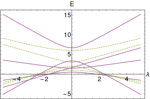
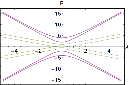
Figure 2: Left: Eigenvalues of the two-qutrit operator $X=C+\lambda L$ for different values of $\lambda$ [see Eqs. (26, 27) for the definitions of $C$ and $L$]. The dotted lines correspond to eigenvalues of entangled eigenstates and the solid lines are depicting eigenvalues of product eigenstates. The lowest and highest eigenstates for the operator $X$ always correspond to product states, yielding a counterexample for the two-qutrit case. Right: Eigenvalues of the qubit-ququart operator $X=C+\lambda L$ for different values of $\lambda$ [see Eqs. (28, 29)]. This gives a counterexample for the qubit-ququart case.

We take $C$ to be diagonal in the computational basis and $|00\rangle$ and $|22\rangle$ are its eigenstates corresponding to the lowest and highest eigenvalues. Requiring that the perturbed ground state remains to be a product state, we get conditions on the entries of the operator $L$. Similarly to Eq. (22) for $k,l>0$ and $m,l<2$ the following must hold:

$$\langle kl|L|00\rangle=\langle ml|L|22\rangle=0.$$ (24)

Since $C$ and $L$ are not diagonal in the same product basis, it follows that the Hermitean operators $L_{A}$ and $L_{B}$ can only have the structure

$$L_{A}=\begin{pmatrix}\centerdot&0&0\\ 0&\centerdot&\centerdot\\ 0&\centerdot&\centerdot\end{pmatrix}\ \ \mbox{and }\ \ L_{B}=\begin{pmatrix}\centerdot&\centerdot&0\\ \centerdot&\centerdot&0\\ 0&0&\centerdot\end{pmatrix},$$ (25)

or the other way round. In fact, choosing the diagonal matrices

$$C_{A}=\begin{pmatrix}1&0&0\\ 0&2&0\\ 0&0&4\end{pmatrix}\ \ \mbox{and }\ \ C_{B}=\begin{pmatrix}\frac{1}{2}&0&0\\ 0&\frac{3}{2}&0\\ 0&0&\frac{5}{3}\end{pmatrix}$$ (26)

and $L_{A}$ and $L_{B}$ to read

$$L_{A}=\left(\begin{array}[]{ccc}1&0&0\\ 0&0&2\\ 0&2&0\end{array}\right)\ \ \mbox{and }\ \ L_{B}=\left(\begin{array}[]{ccc}0&\frac{1}{2}&0\\ \frac{1}{2}&0&0\\ 0&0&1\end{array}\right),$$ (27)

one can explicitly calculate the ground and excited states of $X$ for all $\lambda$. The result is displayed on the left side of Fig. 2. It can be seen that the ground state and the most excited state always correspond to product states.

A similar counterexample can be found for the case of a qubit-ququart system: Choosing

$$C_{A}=\sigma_{z}\ \ \mbox{and }\ \ C_{B}=\begin{pmatrix}2&0&0&0\\ 0&\frac{1}{3}&0&0\\ 0&0&-1&0\\ 0&0&0&4\end{pmatrix}$$ (28)

and

$$L_{A}=\sigma_{x}\ \ \mbox{and }\ \ L_{B}=\begin{pmatrix}3&0&0&0\\ 0&0&1&0\\ 0&1&0&0\\ 0&0&0&3\end{pmatrix},$$ (29)

leads to the eigenvalue structure displayed on right side of Fig. 2.

The presented counterexamples are surprising and relevant for the general construction of entanglement witnesses. In many situations, one tries to identify two product observables, which are easy to measure. Then, in order to obtain a strong witness, a typical recipe is to choose them “locally anticommuting”, meaning that we have $\{C_{X},L_{X}\}=0$ [11]. From our counterexamples we can conclude that in higher dimensions this strategy may not always be successful.

3 Discussion of the results of Ref. [3]

In this section we list the three main statements in Ref. [3] and give a detailed discussion of them. Two of the statements have already been corrected in the erratum [4], but it sometimes remains unclear, where precisely the mistake was made. Therefore, we present the issues in some detail.

First, let us start with Theorem 1 of Ref. [3] for which it has already been pointed out that it requires a revision [4]. The original version of Theorem 1 in Ref. [3] reads: For a given constraint value $c$, the optimal state $\sigma_{\rm opt;\mathcal{X}}\in\mathcal{S}_{\rm sep;\mathcal{X}}$ to the test operator $L$ is a pure state with ${\rm Tr}(C\sigma_{\rm opt;\mathcal{X}})=c$. In the given context $\mathcal{X}=c$ and $\mathcal{S}_{\rm sep;\mathcal{X}}$ denotes all separable states obeying ${\rm Tr}(\varrho{C})=\mathcal{X}$ [see also Eq. (3) in our introduction].

This statement is not correct, when looking for optimal states one cannot restrict the attention to pure states as shown by our counterexample already included in the erratum [4]: Consider a two-qubit system and take the operator $C=|00\rangle\!\langle 00|-|11\rangle\!\langle 11|.$ Then, for any given value $c\in[0,1]$ the state $\varrho_{0}=[(1+c)/2]|00\rangle\!\langle 00|+[(1-c)/2]|11\rangle\!\langle 11|$ is in the plane described by ${\rm Tr}(\varrho{C})=c.$ If one takes the operator $L=|00\rangle\!\langle 00|+|11\rangle\!\langle 11|$ and maximizes its expectation value over pure states in $\mathcal{S}_{\rm sep;c}$ one finds by direct inspection that the value ${\rm Tr}(L\varrho_{0})$ is larger than the value for any pure state in $\mathcal{S}_{\rm sep;c}$.

The error in the proof in Ref. [3] is the following: The range of $\varrho_{0}$ is spanned by the vectors $|00\rangle$ and $|11\rangle$ and there are no other product vectors in the range. These product vectors do not lie in the plane characterized by ${\rm Tr}(\varrho{C})=c$. So, $\varrho_{0}$ constitutes already a counterexample to Lemma 3 in the Supplemental Material. Going deeper, Lemma 2 in the Supplemental Material is also not correct. This Lemma states that a vector $|a^{*}b^{*}\rangle$ occurs in some convex decomposition of $\sigma$, if $|a^{*}b^{*}\rangle$ is not in the kernel of $\sigma^{-1/2}.$ But in the proof it is assumed that $\sigma^{-1/2}\sigma^{1/2}=\mathbbm{1}$, which is not correct if $\sigma$ is not of full rank. Note also that in the original version of this Lemma [12, 13] the condition reads that $|a^{*}b^{*}\rangle$ should be in the range of $\sigma^{-1/2}$.

Closing the discussion concerning Theorem 1, we add that in the erratum [4] Theorem 1 is reformulated and states now correctly that the state $\sigma_{\rm opt;\mathcal{X}}$ is maximally of rank $2$.

Second, we consider Theorem 2 in Ref. [3]. This is ambiguous, as it reads: The necessary condition for the separable operators $C$ and $L$ to detect entanglement […] is that $[C,L]\neq 0$.

The ambiguity comes from the notion of a “separable operator”, which is not defined in Ref. [3]. If one considers operators of the form $C=C_{A}\otimes C_{B}$ to be separable, then the statement is not correct. A counterexample for two qubits are the operators $C=\sigma_{x}\otimes\sigma_{x}$ and $L=\sigma_{z}\otimes\sigma_{z}$. They commute, but can be used for entanglement detection as we have seen in Section II.

In the erratum Theorem 2 is reformulated and the commutator condition is replaced by the condition that the “separable, positive operators” $C$ and $L$ “are not diagonal in a common product basis”. Clearly, the statement is then correct even without a precise notion of “separable” operators, and the positivity of the operators is not required for the conclusion. But the necessary condition is then very weak and far from being sufficient, as we can learn from Proposition 1 in Section III. For instance, if $L=L_{A}\otimes L_{B}$ and $C=C_{A}\otimes C_{B}$ with $[L_{A},C_{A}]=0$ but $[L_{B},C_{B}]\neq 0$, the observables $C$ and $L$ are not diagonal in a common product basis, but they are useless for entanglement detection.

Finally, we consider Corollary 1, which has not been addressed in the erratum: If $C=C_{A}\otimes C_{B}$ and $L=L_{A}\otimes L_{B}$ are product operators, then [in order to be able to detect entanglement] $C_{Y}$ and $L_{Y}$ ($Y=A,B$) must not be jointly measurable.

This statement is not correct. This can be already inferred from Proposition 1 in Section III, but it is very instructive to discuss a counterexample. It can be found by considering noisy versions of Pauli measurements: For $E_{\pm}^{C}=(\mathbbm{1}\pm\sigma_{x}/\sqrt{2})/2$ and $E_{\pm}^{L}=(\mathbbm{1}\pm\sigma_{z}/\sqrt{2})/2$ it is well known that all these effects are jointly measurable [13]. If one takes $C_{Y}=E_{+}^{C}$ and $L_{Y}=E_{+}^{L}$ (for $Y=A,B$) and the corresponding $C$ and $L$ and restricts to the hyperplane $c=0.6$ one can define an ultrafine entanglement witness

$${W}_{\text{UEW}}=g_{c}\mathbbm{1}-{L},$$ (30)

where a value of $g_{c}=0.5223$ can be obtained by a semidefinite program, using the separability criterion of the positivity of the partial transpose. However, one can check that $\hat{W}_{\text{UEW}}$ attains a minimum of $-0.016$ over all states on the hyperplane defined by $c=0.6$. Thus, the jointly measurable operators $C_{Y}$ and $L_{Y}$ are able to detect entanglement via an UEW.

The motivation of this counterexample comes from the fact that

$${W}=\frac{9}{8}\mathbbm{1}-{C}-{L}$$ (31)

is a standard entanglement witness: the expectation value for product states is non-negative, while ${W}$ has a negative eigenvalue. This implies that there must be values of $c$ for which an UEW with $L$ can detect entanglement.

The error in the proof in Ref. [3] is the following. For $E_{\pm}^{C}$ and $E_{\pm}^{L}$ there is a generalized measurement with four outcomes on a qubit that allows to measure them jointly. This generalized measurement can be implemented as a projective measurement $G_{Y}$ on a four-dimensional space, and on this space $C_{Y}$ and $L_{Y}$ have a representation as commuting observables. Then, it is correct that any observed statistics of $G_{A}\otimes G_{B}$ can be mimicked by a separable state (see Eq. 3.1 in the Supplemental Material). But this does not imply that any statistics can be mimicked with a separable state on a $2\times 2$ subsystem (of the total $4\times 4$ space) only, as suggested in the proof of Corollary 1. In other words, if one knows that a state acts on a certain $2\times 2$ subspace only, one can detect entanglement with $G_{A}\otimes G_{B}$.

4 Summary

In summary, we have discussed the problem of entanglement detection, given the expectation values of two observables. We showed that the general problem can be tackled with the method of the Legendre transformation. We identified conditions for two product observables to be useful for entanglement detection. The conditions are necessary and sufficient for two qubits, but the situation in the general case is not clear.

For further work, it would be interesting to clarify in a general setting which combinations of observables are useful for entanglement detection. For instance, it would be interesting to identify three product observables, for which each pair is useless for entanglement detection, but the whole triple is useful. Such examples may then be related to similar studies on joint measurability [14] or state characterization [15].

5 Acknowledgements

We thank T. Heinosaari, M. Ringbauer, F. Shahandeh and R. Uola for discussions. We also thank T. Gühne and D. Wyderka for being quiet sometimes. This work was supported by the DFG and the ERC (Consolidator Grant 683107/TempoQ). M.G. acknowledges funding from the Gesellschaft der Freunde und Förderer der Universität Siegen and N.W. acknowledges funding from the House of Young Talents of the Universität Siegen.

References

References

- [1] R. Horodecki, P. Horodecki, M. Horodecki, and K. Horodecki, Rev. Mod. Phys. 81, 865 (2009).
- [2] O. Gühne and G. Tóth, Phys. Rep. 474, 1 (2009).
- [3] F. Shahandeh, M. Ringbauer, J. C. Loredo, and T.C. Ralph, Phys. Rev. Lett. 118, 110502 (2017), for the erratum see [4].
- [4] F. Shahandeh, M. Ringbauer, J. C. Loredo, and T. C. Ralph, Phys. Rev. Lett. 119, 269901 (2017).
- [5] S.-Q. Shen, T.-R. Xu, S.-M. Fei, X. Li-Jost, and M. Li, Phys. Rev. A 97, 032343 (2018).
- [6] O. Gühne, M. Reimpell, and R.F. Werner, Phys. Rev. Lett. 98, 110502 (2007).
- [7] J. Eisert, F.G.S.L. Brandão, and K.M.R Audenaert, New J. Phys. 9, 46 (2007).
- [8] T.-C. Wei and P.M. Goldbart, Phys. Rev. A 68, 042307 (2003).
- [9] O. Gühne, M. Reimpell, and R.F. Werner, Phys. Rev. A 77, 052317 (2008).
- [10] M. Stingl, Quantentheorie, lecture notes, University of Münster (1997), see www.uni-muenster.de/ Physik.TP/archive/Lehre/Skripten/Stingl/qmskript.ps
- [11] G. Tóth and O. Gühne, Phys. Rev. A 72, 022340 (2005).
- [12] G. Cassinelli, E. De Vito, and A. Levrero, J. Math. Anal. Appl. 210, 472 (1997).
- [13] T. Heinosaari and M. Ziman, The Mathematical Language of Quantum Mechanics, Cambridge University Press (2011).
- [14] C. Heunen, T. Fritz, and M. L. Reyes, Phys. Rev. A 89, 032121 (2014).
- [15] C. Carmeli, T. Heinosaari, J. Schultz, and A. Toigo, Proc. R. Soc. A 473, 20160866 (2017).