Generalisation of Chaplygin’s Reducing Multiplier Theorem with an application to multi-dimensional nonholonomic dynamics

Abstract

A generalisation of Chaplygin’s Reducing Multiplier Theorem is given by providing sufficient conditions for the Hamiltonisation of Chaplygin nonholonomic systems with an arbitrary number $r$ of degrees of freedom via Chaplygin’s multiplier method. The crucial point in the construction is to add an hypothesis of geometric nature that controls the interplay between the kinetic energy metric and the non-integrability of the constraint distribution. Such hypothesis can be systematically examined in concrete examples, and is automatically satisfied in the case $r=2$ encountered in the original formulation of Chaplygin’s theorem. Our results are applied to prove the Hamiltonisation of a multi-dimensional generalisation of the problem of a symmetric rigid body with a flat face that rolls without slipping or spinning over a sphere.

1 Introduction

A substantial amount of research in nonholonomic mechanics in recent years has focused on Hamiltonisation (see e.g. [8, 14, 16, 15, 9, 17, 27, 21, 6, 3, 7] and the references therein). Roughly speaking this is the process by which, via symmetry reduction and a time reparametrisation, the equations of motion of certain nonholonomic systems take a Hamiltonian form.

The Hamiltonisation process has received special attention for the the so-called Chaplygin systems, which are nonholonomic systems with a specific type of symmetry (defined in Section 2). The reduced equations of motion for these systems take the form of an unconstrained mechanical system subject to nonholonomic reaction forces of gyroscopic type. According to [16], it was Appel [2] who first proposed the idea of introducing a time reparametrisation to eliminate these forces, and the idea was taken up by Chaplygin who introduced the reducing multiplier method, and proved his celebrated Reducing Multiplier Theorem [13]. The theorem states that if the reduced space has two degrees of freedom, the reduced equations may be written in Hamiltonian form after a time reparametrisation if and only if there exists an invariant measure. This result has received enormous attention in the community of nonholonomic systems (see e.g. [16, 14, 7] and the references therein) and, despite the low-dimensional restriction on the dimension of the reduced space, it remains to be one of the most solid theoretical results in the area of Hamiltonisation.

On the other hand, in recent years Fedorov and Jovanović have found a remarkable class of examples with arbitrary number of degrees of freedom that allow a Hamiltonisation by Chaplygin’s method [16, 17, 27, 26, 28]. The treatment of the authors in of all these examples is independent of previous theoretical efforts to generalise Chaplygin’s Theorem (e.g. [25, 33, 9, 19]) and the underlying mechanism responsible for the Hamiltonisation of nonholonomic systems with arbitrary number of degrees of freedom remained a mystery.

In this paper we present a generalisation of Chaplygin’s Theorem that gives sufficient conditions for Hamiltonisation via Chaplygin’s method for Chaplygin systems whose reduced space has an arbitrary number $r$ of degrees of freedom. The crucial point is to add hypothesis (H) (see section 3) which is of geometric nature and controls the interplay between the kinetic energy metric and the non-integrability of the constraint distribution. This condition can be systematically analysed in concrete examples and is automatically satisfied in the case $r=2$ considered by Chaplygin.

The usefulness of our generalisation is illustrated by explicitly applying it to prove the Hamiltonisation of a concrete multi-dimensional nonholonomic system. Such system consists of an $n$-dimensional symmetric rigid body with a flat face that rolls without slipping or spinning over an $n-1$-dimensional sphere. This provides a new example of a Hamiltonisable nonholonomic Chaplygin system with arbitrary degrees of freedom.

Geometric interpretation and scope of the results

After the first version of this paper was made available online, some works have appeared that further clarify the underlying geometry and the relevance of the results in this paper.

The first is Gajić and Jovanović [20], that presents a novel application of Chaplygin’s reducing multiplier beyond the nonholonomic setting.

The second is García-Naranjo and Marrero [22], that continues the research started here taking an intrinsic geometric perspective, which shows that our main result is a reformulation of Stanchenko [33, Proposition 2] and Cantrijn et al. [12, Equation (18)]. However, the approach followed in the present paper, and continued in [22], seems to be more convenient to study concrete examples. In fact, [22] also proves that the Hamiltonisation of the multi-dimensional Veselova problem established in [16, 17] may be explained in the light of the results of this paper.

We finally mention García-Naranjo [23] that applies the results of this paper to establish the Hamiltonisation of the multi-dimensional rubber Routh sphere.

Structure of the paper

Section 2 introduces the notation and recalls known results on Chaplygin systems. The formulation and proof of our results is given in Section 3. In section 4 these are applied to prove the Hamiltonisation of our example.

2 Preliminaries

A nonholonomic system consists of a triple $(Q,\mathcal{D},L)$ where $Q$ is an $n$-dimensional configuration manifold, $\mathcal{D}\subset TQ$ is a rank $r$ non-integrable distribution on $Q$ that models $n-r$ independent linear constraints on the velocities, and the Lagrangian $L:TQ\to\mathbb{R}$ is assumed to be of mechanical form, $L=K-U$, where the kinetic energy $K$ defines a Riemannian metric $\langle\cdot,\cdot\rangle$ on $Q$ and $U:Q\to\mathbb{R}$ is the potential energy.

This paper is concerned with nonholonomic $G$-Chaplygin systems, or simply a Chaplygin systems, which are nonholonomic systems $(Q,\mathcal{D},L)$ with the additional property that there is a Lie group $G$ acting freely and properly on $Q$, satisfying the following properties:

1. $G$ acts by isometries on $Q$ and the potential energy $U$ is $G$-invariant,

2. $\mathcal{D}$ is $G$-invariant in the sense that $T_{q}\Phi_{g}(\mathcal{D}_{q})=\mathcal{D}_{\Phi_{g}(q)}$, for all $g\in G$ where $\Phi_{g}:Q\to Q$ is the action diffeomorphism defined by $g$,

3. for every $q\in Q$ the following direct sum splitting holds

   $$T_{q}Q=\mathcal{D}_{q}\oplus(\mathfrak{g}\cdot q),$$ (2.1)

   where $\mathfrak{g}$ denotes the Lie algebra of $G$ and $\mathfrak{g}\cdot q$ the tangent space to the $G$-orbit through $q$.

These systems often appear in applications and have been studied by several authors, e.g. [33, 29, 4, 12, 14, 11]. The reduced configuration manifold $S:=Q/G$ is called the shape space. Note that because of (2.1) the dimension of $S$ coincides with the rank $r$ of $\mathcal{D}$, and the dimension of $G$ is $n-r$.

As first explained by Koiller [29], for Chaplygin systems the constraint distribution $\mathcal{D}$ may be interpreted as the horizontal space of a principal connection on the principal $G$-bundle $\pi:Q\to S$, and the symmetry leads to a reduced system on the space $\mathcal{D}/G$ which is isomorphic to $TS$. The reduced equations on $TS$ take the form of an unconstrained mechanical system on $S$ subject to a gyroscopic force:

$$\frac{d}{dt}\left(\frac{\partial\ell}{\partial\dot{s}^{i}}\right)-\frac{\partial\ell}{\partial s^{i}}=-\sum_{j,k=1}^{r}C^{k}_{ij}(s)\dot{s}^{j}\frac{\partial\ell}{\partial\dot{s}^{k}},\qquad i=1,\dots,r.$$ (2.2)

We now proceed to define the objects in the above equations. First, $(s^{1},\dots,s^{r})$ are local coordinates on $S$. Next, $\ell:TS\to\mathbb{R}$ is the reduced Lagrangian defined by

$$\ell(s,\dot{s})=L\left(q,\mbox{hor}_{q}(\dot{s})\right),\qquad\mbox{where}\quad q\in\pi^{-1}(s),$$ (2.3)

and $\mbox{hor}_{q}(\dot{s})$ denotes the horizontal lift of $\dot{s}\in T_{s}S$ at $q$, which is the tangent vector in $T_{q}Q$ characterised by the conditions that $\mbox{hor}_{q}(\dot{s})\in\mathcal{D}_{q}$ and $T_{q}\pi(\mbox{hor}_{q}(\dot{s}))=\dot{s}$. The reduced Lagrangian is locally written as

$$\ell(s,\dot{s})=\frac{1}{2}\sum_{i,j=1}^{r}K_{ij}(s)\dot{s}^{i}\dot{s}^{j}-U(s),$$ (2.4)

where $U:S\to\mathbb{R}$ now denotes the reduction of the $G$-invariant potential on $Q$, and the coefficients $K_{ij}(s)$ are given by

$$K_{ij}(s)=\left\langle\mbox{ hor}_{q}\left(\frac{\partial}{\partial s^{i}}\right)\,,\,\mbox{ hor}_{q}\left(\frac{\partial}{\partial s^{j}}\right)\right\rangle_{q},\qquad q\in\pi^{-1}(s),$$

and define a Riemannian metric on $S$. As it is standard, we will denote by $K^{ij}(s)$ the entries of the corresponding inverse matrix, i.e.

$$\sum_{k=1}^{r}K_{ik}(s)K^{kj}(s)=\delta_{i}^{j},$$

for all $i,j=1,\dots,r$, where here, and throughout, the symbol $\delta$ is reserved for the Kronecker delta.

Finally, the $s$ dependent coefficients $C_{ij}^{k}$, $i,j,k\in\{1,\dots,r\}$, in (2.2) are locally given by

$$C_{ij}^{k}(s)=\sum_{l=1}^{r}K^{kl}(s)\left\langle\left[\,\mbox{ hor}_{q}\left(\frac{\partial}{\partial s^{i}}\right)\,,\,\mbox{ hor}_{q}\left(\frac{\partial}{\partial s^{j}}\right)\,\right]\,,\,\mbox{ hor}_{q}\left(\frac{\partial}{\partial s^{l}}\right)\right\rangle_{q},\qquad q\in\pi^{-1}(s),$$ (2.5)

where $[\cdot,\cdot]$ denotes the commutator of vector fields on $Q$. Note that they are skew-symmetric on the lower indices, $C_{ij}^{k}=-C_{ji}^{k}$, and as a consequence the energy $E=\sum_{i=1}^{r}\frac{\partial\ell}{\partial\dot{s}^{i}}\dot{s}^{i}-\ell$ is preserved. Inspired by this property we will refer to $C_{ij}^{k}$ as the gyroscopic coefficients.

The gyroscopic coefficients are central to this work. They are the coordinate representation of a $(1,2)$ tensor field on $S$ that we call the gyroscopic tensor

$$\mathcal{T}=\sum_{i,j,k=1}^{r}C_{ij}^{k}(s)\,ds^{i}\otimes ds^{j}\otimes\frac{\partial}{\partial s^{k}}.$$

An intrinsic definition of this tensor, together with a geometric study of its properties in relation to Chaplygin systems is given in García-Naranjo and Marrero [22].

For the rest of the paper we will take a Hamiltonian approach. Define the momenta $p_{i}:=\frac{\partial\ell}{\partial\dot{s}^{i}}$, so that $(s^{1},\dots,s^{r},p_{1},\dots p_{r})$ are canonical coordinates for the cotangent bundle $T^{*}S$. Denote by $H$ the reduced Hamiltonian:

$$H:T^{*}S\to\mathbb{R},\qquad H(s,p)=\sum_{i=1}^{r}p_{i}\dot{s}^{i}-\ell=\frac{1}{2}\sum_{i,j=1}^{r}K^{ij}(s)p_{i}p_{j}+U(s).$$ (2.6)

Equations (2.2) may be rewritten as the following first order system on $T^{*}S$:

$$\frac{ds^{i}}{dt}=\frac{\partial H}{\partial p_{i}},\qquad\frac{dp_{i}}{dt}=-\frac{\partial H}{\partial s^{i}}-\sum_{j,k=1}^{r}C_{ij}^{k}p_{k}\frac{\partial H}{\partial p_{j}},\qquad i=1,\dots,r.$$ (2.7)

2.1 Invariant measures for Chaplygin systems

The existence of a smooth invariant measure for Eqns. (2.7) is intimately related to the condition that a certain 1-form $\Theta$ on $S$ is exact [12, 18]. A local expression for $\Theta$ may be given in terms of the gyroscopic coefficients by:

$$\Theta:=-\sum_{i,j=1}^{r}C_{ij}^{j}\,ds^{i}.$$

In the following theorem recall that $T^{*}S$ is equipped with the Liouville measure $\nu$, that in local bundle coordinates is given by $\nu=ds^{1}\cdots ds^{r}\,dp_{1}\cdots dp_{r}$. Recall also that a volume form $\mu$ on $T^{*}S$ is called a basic measure if its density with respect to $\nu$ does not depend on the momenta $p_{j}$.

Theorem 2.1 (Cantrijn et al. [12]).

Denote by $\nu$ the Liouville volume form on $T^{*}S$ and consider a a mechanical Hamiltonian $H$ given as in (2.6). The reduced equations of motion (2.7) preserve the basic measure

$$\mu=\exp(\sigma)\,\nu,\qquad\sigma\in C^{\infty}(S),$$ (2.8)

if and only if $\Theta$ is exact with $\Theta=d\sigma$.

The proof of the main result of this paper (Theorem 3.4 in section 3 below), uses the fact that $\Theta=d\sigma$ is a necessary condition for the invariance of the measure $\mu$ given by (2.8).

Proof.

In local bundle coordinates,

$$\mu=\exp(\sigma(s))\,ds^{1}\cdots ds^{r}\,dp_{1}\cdots dp_{r}.$$

In view of (2.7), the condition for $\mu$ to be invariant is that

$$\begin{split}0&=\sum_{i=1}^{r}\left[\frac{\partial}{\partial s^{i}}\left(\exp(\sigma(s))\frac{\partial H}{\partial p_{i}}\right)-\frac{\partial}{\partial p_{i}}\left(\exp(\sigma(s))\left(\frac{\partial H}{\partial q^{i}}+\sum_{j,k=1}^{r}C_{ij}^{k}p_{k}\frac{\partial H}{\partial p_{j}}\right)\right)\right]\\ &=\exp(\sigma(s))\sum_{i=1}^{r}\left(\frac{\partial\sigma}{\partial s^{i}}+\sum_{j=1}^{r}C_{ij}^{j}\right)\frac{\partial H}{\partial p_{i}},\end{split}$$

where we have used the skew-symmetry on the lower indices of the coefficients $C_{ij}^{k}$ to cancel the terms involving second derivatives with respect to the momenta. Since the above equality should hold for arbitrary $(s^{1},\dots,s^{r},p_{1},\dots p_{r})$, and (2.6) implies $\frac{\partial H}{\partial p_{i}}=\sum_{j=1}^{r}K^{ij}(s)p_{j}$ where $K^{ij}(s)$ are the coefficients of an invertible matrix, then necessarily

$$\frac{\partial\sigma}{\partial s^{i}}=-\sum_{j=1}^{r}C_{ij}^{j},\qquad i=1,\dots,r,$$ (2.9)

and $\Theta=d\sigma$. The sufficiency of this condition follows immediately from the above analysis. ∎

2.2 Chaplygin’s Reducing Multiplier Method and Theorem

Chaplygin’s reducing multiplier method attempts to find a smooth function $\phi:S\to\mathbb{R}$ such that, after the time and momentum reparametrisation

$$dt=\exp(-\phi(s))\,d\tau,\qquad p_{i}=\exp(-\phi(s))\,\tilde{p}_{i},\qquad i=1,\dots,r,$$

the equations of motion (2.7) transform into Hamiltonian form:

$$\frac{ds^{i}}{d\tau}=\frac{\partial\tilde{H}}{\partial\tilde{p}_{i}},\qquad\frac{d\tilde{p}_{i}}{d\tau}=-\frac{\partial\tilde{H}}{\partial s^{i}},\qquad i=1,\dots,r,$$ (2.10)

where $\tilde{H}(s_{i},\tilde{p}_{i})=H(s_{i},\exp(-\phi(s))\,\tilde{p}_{i})$. The process described above is often termed Chaplygin Hamiltonisation. The contribution of this paper is to give sufficient conditions for the existence of $\phi$ that can be systematically examined in concrete examples. Here we recall two well-established results. The first one is that the existence of a basic, smooth invariant measure is a necessary condition for Chaplygin Hamiltonisation (see e.g. [16] and [14]).

Proposition 2.2.

Suppose that a nonholonomic Chaplygin system allows a Chaplygin Hamiltonisation by the time and momentum reparametrisation

$$dt=\exp(-\phi(s))\,d\tau,\qquad p_{i}=\exp(-\phi(s))\,\tilde{p}_{i},\qquad i=1,\dots,r.$$

Then, its reduced equations of motion (2.7) possess the invariant measure $\mu=\exp(\sigma(s))\,\nu$, where $\nu$ is the Liouville volume form on $T^{*}S$ and $\sigma=(r-1)\phi$.

Proof.

By Liouville’s Theorem, the transformed equations (2.10) preserve the measure

$$\begin{split}\tilde{\mu}&=ds^{1}\wedge\cdots\wedge ds^{r}\wedge d\tilde{p}_{1}\wedge\cdots\wedge d\tilde{p}_{r}\\ &=\exp(r\phi(s))\,ds^{1}\wedge\cdots\wedge ds^{r}\wedge dp_{1}\wedge\cdots\wedge dp_{r}.\end{split}$$

Therefore, the equations in the original time variable $t$ preserve the measure $\mu=\exp(-\phi(s))\tilde{\mu}$. ∎

The celebrated Chaplygin’s Reducing Multiplier Theorem establishes that if the dimension of the shape space is 2, the existence of the invariant measure $\mu=\exp(\sigma(s))\,\nu$ is not only necessary, but also sufficient for Chaplygin Hamiltonisation. More precisely:

Theorem 2.3 (Chaplygin’s Reducing Multiplier Theorem [13]).

Suppose that $r=2$ and that the reduced equations (2.7) possess the invariant measure

$$\mu=\exp(\sigma(s))\,\nu,\qquad\sigma\in C^{\infty}(S),$$

where $\nu$ is the Liouville volume form on $T^{*}S$. Then after the time and momentum reparametrisation

$$dt=\exp(-\sigma(s))\,d\tau,\qquad p_{i}=\exp(-\sigma(s))\,\tilde{p}_{i},\qquad i=1,2,$$

the equations (2.7) transform to Hamiltonian form

$$\frac{ds^{i}}{d\tau}=\frac{\partial\tilde{H}}{\partial\tilde{p}_{i}},\qquad\frac{d\tilde{p}_{i}}{d\tau}=-\frac{\partial\tilde{H}}{\partial s_{i}},\qquad i=1,2,$$

where $\tilde{H}(s^{i},\tilde{p}_{i})=H(s^{i},\exp(-\sigma(s))\tilde{p}_{i})$.

The theorem of Chaplygin is a particular instance of our main Theorem 3.4 given below.

3 Generalisation of Chaplygin’s Reducing Multiplier Theorem

The generalisation of Chaplygin’s Theorem 2.3 that we present gives sufficient conditions for the Hamiltonisation of Chaplygin systems whose shape space $S$ has dimension $r\geq 2$. We replace the low dimensional assumption on $S$ of Chaplygin’s Theorem, by the following hypothesis on the gyroscopic coefficients $C_{ij}^{k}$:

(H).

The gyroscopic coefficients $C_{ij}^{k}$ satisfy

$$C_{ij}^{k}=0,\quad\mbox{for}\quad k\neq i\neq j\neq k,\qquad C_{ij}^{j}=C_{ik}^{k}\quad\mbox{for all }\quad j,k\neq i.$$

It may seem that condition (H), as formulated here, depends on the choice of coordinates. Lemma 3.3 below shows that this is not the case.

Remark 3.1.

It is immediate to check that (H) is satisfied automatically if $r=2$.

Remark 3.2.

In the proofs of Lemma 3.3 and Theorem 3.4 below, we will find it useful to work with the following, equivalent formulation of condition (H):

$$C_{ij}^{k}=\chi_{i}\delta_{j}^{k}-\chi_{j}\delta_{i}^{k},$$ (3.1)

for certain locally defined functions $\chi_{i}$ on $S$, $i=1,\dots r$.

Lemma 3.3.

Let $(s^{1},\dots,s^{r})$ and $(y^{1},\dots,y^{r})$ be coordinates on a neighbourhood of $S$, and let $C_{ij}^{k}$ and $\tilde{C}_{\alpha\beta}^{\gamma}$ be the corresponding gyroscopic coefficients. If $C_{ij}^{k}$ satisfy (H), then the same is true about $\tilde{C}_{\alpha\beta}^{\gamma}$.

Proof.

Due to the coordinate transformation rules for the gyroscopic tensor $\mathcal{T}$ we have

$$\tilde{C}_{\alpha\beta}^{\gamma}=\sum_{i,j,k=1}^{r}C_{ij}^{k}\frac{\partial s^{i}}{\partial y^{\alpha}}\frac{\partial s^{j}}{\partial y^{\beta}}\frac{\partial y^{\gamma}}{\partial s^{k}},\quad\mbox{for all}\quad\alpha,\beta,\gamma=1,\dots,r.$$

Hence, (3.1) implies

$$\begin{split}\tilde{C}_{\alpha\beta}^{\gamma}&=\sum_{i,j=1}^{r}\left(\chi_{i}\frac{\partial s^{i}}{\partial y^{\alpha}}\frac{\partial s^{j}}{\partial y^{\beta}}\frac{\partial y^{\gamma}}{\partial s^{j}}\right)-\sum_{i,j=1}^{r}\left(\chi_{j}\frac{\partial s^{i}}{\partial y^{\alpha}}\frac{\partial s^{j}}{\partial y^{\beta}}\frac{\partial y^{\gamma}}{\partial s^{i}}\right)\\ &=\left(\sum_{i=1}^{r}\chi_{i}\frac{\partial s^{i}}{\partial y^{\alpha}}\right)\delta^{\gamma}_{\beta}-\left(\sum_{j=1}^{r}\chi_{j}\frac{\partial s^{j}}{\partial y^{\beta}}\right)\delta^{\gamma}_{\alpha}.\end{split}$$

Therefore, the coefficients $\tilde{C}_{\alpha\beta}^{\gamma}$ also satisfy (3.1) with corresponding $\tilde{\chi}_{\alpha}=\sum_{i=1}^{r}\chi_{i}\frac{\partial s^{i}}{\partial y^{\alpha}}$. ∎

The lemma shows that (H) contains intrinsic geometric information about the interplay between the kinetic energy metric and the constraint distribution (see Remark 3.5 below for more details).

Recall from Proposition 2.2 that the existence of a basic invariant measure is a necessary condition for Chaplygin Hamiltonisation. Moreover, its density with respect to the Liouville volume determines the corresponding time and momentum rescaling. Our main result, stated in the theorem below, shows that, in the presence of a basic invariant measure, the Chaplygin Hamiltonisation of the system is guaranteed by condition (H).

Theorem 3.4 (Generalisation of Chaplygin’s Reducing Multiplier Theorem).

Suppose that $r\geq 2$ and that the reduced equations (2.7) possess the invariant measure

$$\mu=\exp(\sigma(s))\,\nu,\qquad\sigma\in C^{\infty}(S),$$

where $\nu$ is the Liouville volume form on $T^{*}S$. Suppose moreover that the gyroscopic coefficients satisfy (H) everywhere on $S$. Then, after the time and momentum reparametrisation

$$dt=\exp\left(\frac{\sigma(s)}{1-r}\right)\,d\tau,\qquad p_{i}=\exp\left(\frac{\sigma(s)}{1-r}\right)\,\tilde{p}_{i},\qquad i=1,\dots,r,$$ (3.2)

the equations (2.7) transform to Hamiltonian form

$$\frac{ds^{i}}{d\tau}=\frac{\partial\tilde{H}}{\partial\tilde{p}_{i}},\qquad\frac{d\tilde{p}_{i}}{d\tau}=-\frac{\partial\tilde{H}}{\partial s_{i}},\qquad i=1,\dots,r,$$

where $\tilde{H}(s^{i},\tilde{p}_{i})=H\left(s^{i},\exp\left(\frac{\sigma(s)}{1-r}\right)\,\tilde{p}_{i}\right)$.

Since (H) holds automatically when $r=2$ (Remark 3.1), this is indeed a generalisation of Chaplygin’s Theorem 2.3.

Proof.

By the chain rule we have

$$\frac{\partial\tilde{H}}{\partial s^{i}}=\frac{\partial H}{\partial s^{i}}+\frac{1}{1-r}\sum_{j=1}^{r}\frac{\partial H}{\partial p_{j}}\tilde{p}_{j}\exp\left(\frac{\sigma(s)}{1-r}\right)\frac{\partial\sigma}{\partial s^{i}},\qquad\frac{\partial\tilde{H}}{\partial\tilde{p}_{i}}=\exp\left(\frac{\sigma(s)}{1-r}\right)\frac{\partial H}{\partial p_{i}},$$

and hence

$$\frac{\partial H}{\partial s^{i}}=\frac{\partial\tilde{H}}{\partial s^{i}}-\frac{1}{1-r}\sum_{j=1}^{r}\frac{\partial\tilde{H}}{\partial\tilde{p}_{j}}\tilde{p}_{j}\frac{\partial\sigma}{\partial s^{i}},\qquad\frac{\partial H}{\partial p_{i}}=\exp\left(\frac{-\sigma(s)}{1-r}\right)\frac{\partial\tilde{H}}{\partial\tilde{p}_{i}},\qquad i=1,\dots,r.$$ (3.3)

Therefore, in view of the first equation in (2.7) we obtain

$$\frac{ds^{i}}{d\tau}=\exp\left(\frac{\sigma(s)}{1-r}\right)\frac{ds^{i}}{dt}=\frac{\partial\tilde{H}}{\partial\tilde{p}_{i}},\qquad i=1,\dots,r.$$ (3.4)

On the other hand we have

$$\begin{split}\frac{d\tilde{p}_{i}}{d\tau}&=\exp\left(\frac{\sigma(s)}{1-r}\right)\frac{d\tilde{p}_{i}}{dt}=\frac{dp_{i}}{dt}-\frac{p_{i}}{1-r}\sum_{j=1}^{r}\frac{\partial\sigma}{\partial s_{j}}\frac{ds^{j}}{dt}.\end{split}$$

Using now both equations in (2.7), the above equation becomes

$$\frac{d\tilde{p}_{i}}{d\tau}=-\frac{\partial H}{\partial s^{i}}-\sum_{j,k=1}^{r}C_{ij}^{k}p_{k}\frac{\partial H}{\partial p_{j}}-\frac{p_{i}}{1-r}\sum_{j=1}^{r}\frac{\partial\sigma}{\partial s_{j}}\frac{\partial H}{\partial p_{j}},$$ (3.5)

which in view of (3.3) gives

$$\frac{d\tilde{p}_{i}}{d\tau}=-\frac{\partial\tilde{H}}{\partial s^{i}}+\sum_{j=1}^{r}\left[\frac{1}{1-r}\left(\tilde{p}_{j}\frac{\partial\sigma}{\partial s^{i}}-\tilde{p}_{i}\frac{\partial\sigma}{\partial s^{j}}\right)-\sum_{k=1}^{r}C_{ij}^{k}\tilde{p}_{k}\right]\frac{\partial\tilde{H}}{\partial\tilde{p}_{j}},\qquad i=1,\dots,r.$$ (3.6)

Using that (H) holds, we use (3.1) to simplify

$$\sum_{k=1}^{r}C_{ij}^{k}\tilde{p}_{k}=\tilde{p}_{j}\chi_{i}-\tilde{p}_{i}\chi_{j}.$$ (3.7)

On the other hand, the assumption that the measure $\mu$ is preserved by the flow, implies, by Theorem 2.1, that (2.9) holds. Combining these equations with (H) formulated as (3.1), we have

$$\begin{split}\tilde{p}_{j}\frac{\partial\sigma}{\partial s^{i}}-\tilde{p}_{i}\frac{\partial\sigma}{\partial s^{j}}&=-\tilde{p}_{j}\sum_{k=1}^{r}C_{ik}^{k}+\tilde{p}_{i}\sum_{k=1}^{r}C_{jk}^{k}=-\tilde{p}_{j}\sum_{k=1,k\neq i}^{r}\chi_{i}+\tilde{p}_{i}\sum_{k=1,k\neq j}^{r}\chi_{j}\\ &=(r-1)\left(\tilde{p}_{i}\chi_{j}-\tilde{p}_{j}\chi_{i}\right).\end{split}$$ (3.8)

Substitution of (3.7) and (3.8) into (3.6) leads to $\frac{d\tilde{p}_{i}}{d\tau}=-\frac{\partial\tilde{H}}{\partial s^{i}}$, for $i=1,\dots,r$, as required. ∎

Remark 3.5.

The notion of $\phi$-simple Chaplygin systems introduced in [22] gives a coordinate free characterisation of the systems that satisfy the hypothesis of Theorem 3.4. Such concept is inspired by the observation that (H) is equivalent to the the existence of a 1-form $\chi$ on $S$ such that

$$\mathcal{T}(Y,Z)=\chi(Y)Z-\chi(Z)Y,$$

for any two vector fields $Y,Z$ on $S$.

Remark 3.6.

The reduced equations of motion (2.7) may be formulated in almost Hamiltonian form with respect to a 2-form on $T^{*}S$ that is non-degenerate but fails to be closed [33, 14]. An equivalent geometric formulation of Theorem 3.4 states that such 2-form is closed after multiplication by the conformal factor $f(s)=\exp\left(\frac{\sigma(s)}{r-1}\right)$, see [22].

Our result on Chaplygin Hamiltonisation persists under the addition of an invariant potential. More precisely we have:

Corollary 3.7.

Suppose that a $G$-Chaplygin system satisfies the hypothesis of Theorem 3.4. Then, after the addition of a $G$-invariant potential energy, the system continues to satisfy the hypothesis of Theorem 3.4 so it allows a Chaplygin Hamiltonisation by the same reparametrisation of time and momenta.

Proof.

It is immediate to see from (2.7) that the system with the extra potential preserves the same volume form. On the other hand, the system with the extra potential also satisfies condition (H) since the definition of the gyroscopic coefficients is independent of the potential. ∎

4 Example: Hamiltonisation of a multi-dimensional symmetric rigid body with a flat face that rubber rolls on the outer surface of a sphere

Following Borisov et al [10], consider the motion of a rigid body with a flat face which is at every time tangent to a sphere of radius $R$ that is fixed in space, see Figure 4.1. The body is subject to a rolling nonholonomic constraint that prevents slipping of its flat face over the surface of sphere, and to a rubber nonholonomic constraint that prohibits spinning, namely it forbids rotations of the body about the normal vector to the sphere at the contact point $P$. This problem without the rubber constraint was first considered by Woronets [34, 35].

We shall give a multi-dimensional generalisation of the system and, assuming some symmetry of the body, prove its Hamiltonisation by applying Theorem 3.4.

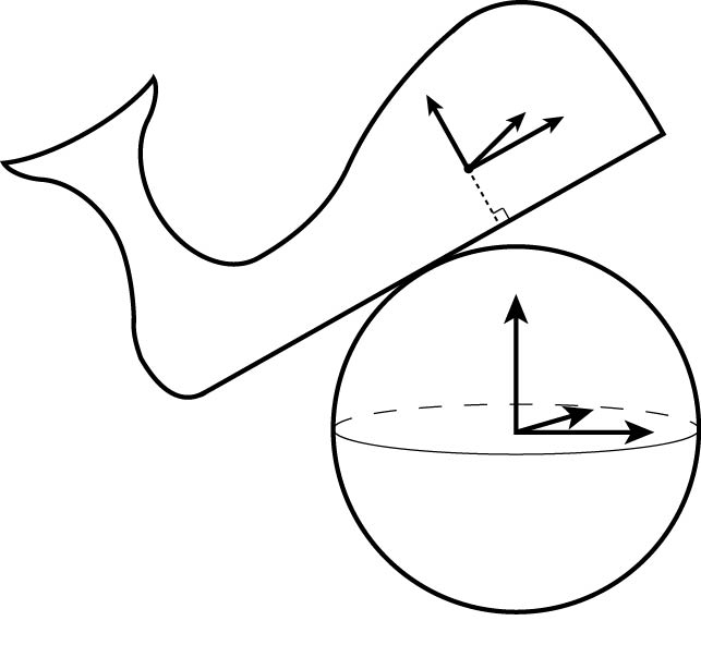
Figure 4.1: Body with a flat face that rubber rolls over a fixed sphere.

4.1 The 3-dimensional case

Consider a moving body frame $\{E_{1},E_{2},E_{3}\}$ that is rigidly attached to the body at its centre of mass $C$ and is such that the $E_{3}$ axis is parallel to the outward normal vector to the sphere at the contact point $P$ (see Figure 4.1). Consider also a fixed space frame $\{e_{1},e_{2},e_{3}\}$ which is attached to the centre $O$ of the sphere. As usual, the change of basis matrix between the two coordinate systems is an element $g\in\mathrm{SO}(3)$ that determines the attitude of the body.

Let $x=(x_{1},x_{2},x_{3})^{T}\in\mathbb{R}^{3}$ be the space coordinates of the vector $\overrightarrow{OC}$. Its corresponding body coordinates are

$$X=(X_{1},X_{2},X_{3})^{T}=g^{-1}x.$$ (4.1)

The condition that the flat face of the body is always tangent to the sphere gives the holonomic constraint

$$X_{3}=R+a,$$ (4.2)

where $a$ is the distance between $C$ and the flat face, positively measured in the direction of $E_{3}$.

The configuration of the system is completely determined by $((X_{1},X_{2}),g)\in\mathbb{R}^{2}\times\mathrm{SO}(3)$ so the configuration space is $Q=\mathbb{R}^{2}\times\mathrm{SO}(3)$. In particular, the space coordinates of the vector $\overrightarrow{OP}$ are the entries of the vector $RgE_{3}$.

Let $\Omega=(\Omega_{1},\Omega_{2},\Omega_{3})^{T}\in\mathbb{R}^{3}$ be the angular velocity of the body written in the body frame. Then

$$g^{-1}\dot{g}=\begin{pmatrix}0&-\Omega_{3}&\Omega_{2}\\ \Omega_{3}&0&-\Omega_{1}\\ -\Omega_{2}&\Omega_{1}&0\end{pmatrix}\in\mathfrak{so}(3).$$ (4.3)

The constraint that the body rolls without slipping over the sphere is

$$\dot{X}=-R\Omega\times E_{3},$$ (4.4)

where $\times$ denotes the usual cross product in $\mathbb{R}^{3}$. On the other hand, the rubber constraint is

$$\Omega_{3}=0.$$ (4.5)

Consider the motion of the body in the absence of potential forces, so the Lagrangian is given by the kinetic energy. Let $\|\cdot\|$ denote the euclidean norm in $\mathbb{R}^{3}$. Considering that $\|\dot{x}\|^{2}=\|g^{-1}\dot{x}\|^{2}$ and

$$g^{-1}\dot{x}=\dot{X}+\Omega\times X,$$

we have

$$L:TQ\to\mathbb{R},\qquad L(X,g,\dot{X},\dot{g})=\frac{1}{2}(\mathbb{I}\Omega,\Omega)+\frac{m}{2}\left\|\dot{X}+\Omega\times X\right\|^{2},$$ (4.6)

where $m$ is the total mass of the body, $\mathbb{I}$ is the inertia tensor and $(\cdot,\cdot)$ is the euclidean scalar product in $\mathbb{R}^{3}$. In the above equation it is understood that $X_{3}=R+a$ and $\dot{X}_{3}=0$.

There is a freedom in the choice of orientation of the space frame which is represented by the action of $\mathrm{SO}(3)$ on $Q$ given by $h\cdot((X_{1},X_{2}),g)=((X_{1},X_{2}),hg)$. It is easily verified that this action satisfies the conditions (i)–(iii), given in the definition of a Chaplygin system in Section 2. Therefore, our problem is an $\mathrm{SO}(3)$-Chaplygin system with shape space $S=\mathbb{R}^{2}$.

It was shown by Borisov et al [10] that the system possesses a smooth invariant measure if and only if the mass distribution of the body is such that at least one of the following conditions is satisfied:

• The inertia tensor $\mathbb{I}=\mbox{diag}(I_{1},I_{2},I_{3})$ and $a=0$.

• The inertia tensor $\mathbb{I}=\mbox{diag}(I_{1},I_{1},I_{3})$.

Since the shape space $S=\mathbb{R}^{2}$ is two-dimensional, the Hamiltonisation of the system if either C1 or C2 holds follows from Chaplygin’s Reducing Multiplier Theorem 2.3.

Remark 4.1.

Note that the inertia tensor in C1 is non-generic since an assumption on the orientation of the body frame has already been made. The condition C2 says that the body is axially symmetric about an axis perpendicular to the flat face.

4.2 The $n$-dimensional case

The multi-dimensional generalisation of the system treated in the previous section consists of an $n$-dimensional rigid body with a flat $n-1$-dimensional face that rolls without slipping or spinning about a fixed $n-1$-dimensional sphere of radius $R$ centred at $O$ in $\mathbb{R}^{n}$. We follow the notation of the previous section. Most of the formulas admit a straightforward generalisation.

As before, assume that the body frame $\{E_{1},\dots,E_{n}\}$ is attached to the centre of mass $C$ of the body and $E_{n}$ is parallel to the outward normal vector to the sphere at the contact point. The space frame $\{e_{1},\dots,e_{n}\}$ has its origin at $O$.

The $n^{th}$ entry of the vector $X\in\mathbb{R}^{n}$, that gives body coordinates of the vector $\overrightarrow{OC}$, satisfies the holonomic constraint

$$X_{n}=R+a,$$ (4.7)

that generalises (4.2). The configuration space of the system is

$$Q=\mathbb{R}^{n-1}\times\mathrm{SO}(n)\ni((X_{1},\dots,X_{n-1}),g),$$

where the attitude matrix $g$ is the change of basis matrix between the body and the space frame. The angular velocity in the body frame is the skew symmetric matrix

$$\Omega=g^{-1}\dot{g}\in\mathfrak{so}(n),$$

with entries $\Omega_{\mu\nu}$, $1\leq\mu,\nu\leq n$. The rolling constraints (4.4) generalise to

$$\dot{X}=-R\Omega E_{n},$$ (4.8)

which in particular imply $\dot{X}_{n}=0$ in consistency with (4.7). On the other hand, the natural generalisation of the rubber constraints (4.5) that prohibit spinning is

$$\Omega_{\mu\nu}=0,\qquad 1\leq\mu,\nu\leq n-1.$$ (4.9)

Now recall that for an $n$-dimensional rigid body the inertia tensor $\mathbb{I}$ of the body is an operator

$$\mathbb{I}:\mathfrak{so}(n)\to\mathfrak{so}(n),\qquad\mathbb{I}(\Omega)=\mathbb{J}\Omega+\Omega\mathbb{J},$$

where $\mathbb{J}$ is the so-called mass tensor of the body, which is a symmetric and positive definite $n\times n$ matrix (see e.g. [32]). The Lagrangian is

$$L:TQ\to\mathbb{R},\qquad L(X,g,\dot{X},\dot{g})=\frac{1}{2}(\mathbb{I}\Omega,\Omega)_{\kappa}+\frac{m}{2}\left\|\dot{X}+\Omega X\right\|^{2},$$ (4.10)

where $\|\cdot\|$ is the euclidean norm in $\mathbb{R}^{n}$, $X=(X_{1},\dots,X_{n-1},R+a)$, $\dot{X}_{n}=0$, and $(\cdot,\cdot)_{\kappa}$ is the Killing metric in $\mathfrak{so}(n)$:

$$(\xi,\eta)_{\kappa}=-\frac{1}{2}\mathop{\mathrm{missing}}{tr}\nolimits(\xi\eta).$$

In analogy with the 3-dimensional case, it is easy to establish that the multi-dimensional problem is an $\mathrm{SO}(n)$-Chaplygin system with $r=n-1$-dimensional shape space $S=\mathbb{R}^{n-1}$. The following theorem generalises the situation that was found in the $3$-dimensional case.

Theorem 4.2.

Let $n\geq 3$. The reduced system on $T^{*}\mathbb{R}^{n-1}$ possesses an invariant measure and is Hamiltonisable if any of the following two conditions hold

• The mass tensor $\mathbb{J}=\mbox{\em diag}(J_{1},J_{2},\dots,J_{n})$ and $a=0$.

• The mass tensor $\mathbb{J}=\mbox{\em diag}(J_{1},\dots,J_{1},J_{n})$.

Note that a multi-dimensional generalisation of Remark 4.1 also applies.

Proof.

The proof is an application of Theorem 3.4. The main task is to compute the gyroscopic coefficients $C_{ij}^{k}$ in the coordinates

$$s_{i}=X_{i},\qquad i=1,\dots,n-1,$$

that provide a global chart for $S=\mathbb{R}^{n-1}$. The proof of the following lemma is given at the end of the section.

Lemma 4.3.

The gyroscopic coefficients $C_{ij}^{k}$ written in the coordinates $(s_{1},\dots,s_{n-1})$ are given as follows in the cases C1 and C2 described in Theorem 4.2:

• $C_{ij}^{k}=0$ for all $i,j,k\in\{1,\dots,n-1\}$.

• $$C_{ij}^{k}=\frac{-ma}{R(J_{1}+J_{n}+ma^{2})}(s_{i}\delta_{j}^{k}-s_{j}\delta_{i}^{k}),\qquad 1\leq i,j,k\leq n-1.$$ (4.11)

It follows from the lemma that if C1 holds, then the reduced system (2.7) is already Hamiltonian without the need of a time reparametrisation, and the symplectic volume form on $T^{*}\mathbb{R}^{n-1}$ is preserved. A similar phenomenon is encountered in the example of a homogeneous vertical disk that rolls on the plane (see e.g. [5, 22]).

On the other hand, if C2 holds, then (4.11) implies that (H) is verified and (3.1) holds with $\chi_{i}=\frac{-ma}{R(J_{1}+J_{n}+ma^{2})}s_{i}$. Moreover, the conditions (2.9) for the preservation of the measure $\mu=\exp(\sigma(s))\,\nu$ are satisfied with

$$\sigma=\frac{(n-2)ma}{2R(J_{1}+J_{n}+ma^{2})}\sum_{i=1}^{n-1}s_{i}^{2}.$$

Therefore, Theorem 3.4 applies and the system is also Hamiltonisable in this case. ∎

The details about the Hamiltonisation stated in Theorem 4.2 are given in the following corollary that is a direct consequence of the proof given above.

Corollary 4.4.

If the condition C1 in Theorem 4.2 holds, then the reduced equations of motion on $T^{*}\mathbb{R}^{n-1}$ are Hamiltonian in the natural time variable and preserve the Liouville measure $\nu$ in $T^{*}\mathbb{R}^{n-1}$.

If the condition C2 in Theorem 4.2 holds, then the reduced equations of motion on $T^{*}\mathbb{R}^{n-1}$ preserve the measure

$$\mu=\exp\left(\frac{(n-2)ma}{2R(J_{1}+J_{n}+ma^{2})}\sum_{i=1}^{n-1}X_{i}^{2}\right)\,\nu,$$

and become Hamiltonian after the time and momentum reparametrisation

$$\begin{split}dt&=\exp\left(\frac{-ma}{2R(J_{1}+J_{n}+ma^{2})}\sum_{i=1}^{n-1}X_{i}^{2}\right)\,d\tau,\\ p_{i}&=\exp\left(\frac{-ma}{2R(J_{1}+J_{n}+ma^{2})}\sum_{i=1}^{n-1}X_{i}^{2}\right)\,\tilde{p}_{i},\qquad i=1,\dots,n-1.\end{split}$$

We finally present:

Proof of Lemma 4.3.

Throughout the proof, for $u,v\in\mathbb{R}^{n}$ we denote

$$u\wedge v=uv^{T}-vu^{T}\in\mathfrak{so}(n).$$

The constraints (4.8) and (4.9) imply

$$\Omega=-\frac{1}{R}\dot{X}\wedge E_{n}.$$ (4.12)

In what follows, we abbreviate $s=(s_{1},\dots,s_{n-1})\in\mathbb{R}^{n-1}$ and $\tilde{s}=(s,R+a)\in\mathbb{R}^{n}$.

For $q=(s,g)\in Q$, identify $T_{q}Q=\mathbb{R}^{n}\times\mathfrak{so}(n)$ using the the left trivialisation of $T_{g}\mathrm{SO}(n)$ and the standard identifications and imbedding $T_{s}\mathbb{R}^{n-1}=\mathbb{R}^{n-1}=\mathbb{R}^{n-1}\times\{0\}\hookrightarrow\mathbb{R}^{n}$.

Equation (4.12) implies that:

$$\mbox{ hor}_{q}\left(\frac{\partial}{\partial s_{i}}\right)=\left(E_{i},-\frac{1}{R}E_{i}\wedge E_{n}\right),\qquad i=1,\dots,n-1.$$

As before, denote by $\langle\cdot,\cdot\rangle$ the Riemannian metric on $Q$ defined by the kinetic energy Lagrangian (4.10). We have

$$\begin{split}K_{kl}(s)&=\left\langle\mbox{ hor}_{q}\left(\frac{\partial}{\partial s_{k}}\right),\mbox{ hor}_{q}\left(\frac{\partial}{\partial s_{l}}\right)\right\rangle_{q}\\ &=\frac{1}{R^{2}}(\mathbb{I}(E_{k}\wedge E_{n}),E_{l}\wedge E_{n})_{\kappa}+m\left(E_{k}-\frac{1}{R}(E_{k}\wedge E_{n})\tilde{s},E_{l}-\frac{1}{R}(E_{l}\wedge E_{n})\tilde{s}\right)_{\mathbb{R}^{n}},\end{split}$$

where $(\cdot,\cdot)_{\mathbb{R}^{n}}$ denotes the euclidean inner product in $\mathbb{R}^{n}$. Performing the calculations the above expression simplifies to

$$K_{kl}(s)=\frac{1}{R^{2}}\left(\mathbb{J}_{kl}+ms_{k}s_{l}+(\mathbb{J}_{nn}+ma^{2})\delta_{kl}\right),\qquad 1\leq k,l\leq n-1.$$ (4.13)

On the other hand the commutator

$$\left[\mbox{ hor}_{q}\left(\frac{\partial}{\partial s_{i}}\right),\mbox{ hor}_{q}\left(\frac{\partial}{\partial s_{j}}\right)\right]=\frac{1}{R^{2}}\left(0,[E_{i}\wedge E_{n},E_{j}\wedge E_{n}]_{\mathfrak{so}(n)}\right)=-\frac{1}{R^{2}}\left(0,E_{i}\wedge E_{j}\right),\quad 1\leq i,j\leq n-1,$$

where $[\cdot,\cdot]_{\mathfrak{so}(n)}$ is the Lie algebra commutator in $\mathfrak{so}(n)$. Whence,

$$\begin{split}&\left\langle\left[\mbox{ hor}_{q}\left(\frac{\partial}{\partial s_{i}}\right),\mbox{ hor}_{q}\left(\frac{\partial}{\partial s_{j}}\right)\right]\,,\,\mbox{ hor}_{q}\left(\frac{\partial}{\partial s_{l}}\right)\right\rangle_{q}\\ &\qquad\qquad\qquad=\frac{1}{R^{3}}(\mathbb{I}(E_{i}\wedge E_{j}),E_{l}\wedge E_{n})_{\kappa}+m\left(-\frac{1}{R^{2}}(E_{i}\wedge E_{j})\tilde{s},E_{l}-\frac{1}{R}(E_{l}\wedge E_{n})\tilde{s}\right)_{\mathbb{R}^{n}}.\end{split}$$

Under the assumption that $\mathbb{J}$ is diagonal, the above expression simplifies to

$$\left\langle\left[\mbox{ hor}_{q}\left(\frac{\partial}{\partial s_{i}}\right),\mbox{ hor}_{q}\left(\frac{\partial}{\partial s_{j}}\right)\right]\,,\,\mbox{ hor}_{q}\left(\frac{\partial}{\partial s_{l}}\right)\right\rangle_{q}=\frac{ma}{R^{3}}(s_{j}\delta_{il}-s_{i}\delta_{jl}),\qquad 1\leq i,j,l\leq n-1.$$ (4.14)

If C1 holds then $a=0$ and all of the gyroscopic coefficients $C_{ij}^{k}$ vanish in view of (2.5).

It remains to consider the case C2. Assume thus that $\mathbb{J}=(J_{1},\dots,J_{1},J_{n})$. Then (4.13) simplifies to

$$K_{kl}(s)=\frac{1}{R^{2}}\left((J_{1}+J_{n}+ma^{2})\delta_{kl}+ms_{k}s_{l}\right),\qquad 1\leq k,l\leq n-1,$$

and hence, the coefficients $C_{ij}^{k}(s)$ defined by (4.11) satisfy

$$\begin{split}\sum_{k=1}^{n-1}K_{kl}(s)C_{ij}^{k}(s)&=\frac{ma}{R(J_{1}+J_{n}+ma^{2})}(-K_{jl}s_{i}+K_{il}s_{j})\\ &=\frac{ma}{R^{3}}\left(-s_{i}\delta_{jl}+s_{j}\delta_{il}\right)\\ &=\left\langle\left[\mbox{ hor}_{q}\left(\frac{\partial}{\partial s_{i}}\right),\mbox{ hor}_{q}\left(\frac{\partial}{\partial s_{j}}\right)\right]\,,\,\mbox{ hor}_{q}\left(\frac{\partial}{\partial s_{l}}\right)\right\rangle_{q},\end{split}$$

where the last identity follows from (4.14). This completes the proof since the above equation is equivalent to (2.5). ∎

Acknowledgements: I acknowledge the Alexander von Humboldt Foundation for a Georg Forster Experienced Researcher Fellowship that funded a research visit to TU Berlin where this work was done.

I am extremely grateful to Y. Suris for numerous conversations during my research stay at TU Berlin. It was him who, in the course of these conversations, recognised the potential relevance of hypothesis (H) and encouraged me to investigate it further.

I also thank J. Koiller and Y. Fedorov for their comments on an early version of this paper and J.C. Marrero for conversations that were useful to understand the intrinsic character of the gyroscopic coefficients. I thank C. Fernández for her help to produce Figure 4.1.

Finally, I express my gratitude to the anonymous referees of the paper who helped me improve the exposition with their useful comments and remarks.

LGN: Departamento de Matemáticas y Mecánica, IIMAS-UNAM. Apdo. Postal 20-126, Col. San Ángel, Mexico City, 01000, Mexico. luis@mym.iimas.unam.mx

References

- [1]
-
[2]
Appel P.
Remarques d’orde analytique sur un nouvelle forme des equationes de la dynamique. J. Math. Pure Appl. 7 (1901), ser. 5, 5–12. -
[3]
Balseiro P. and L.C. García-Naranjo
Gauge transformations, twisted Poisson brackets and Hamiltonization of nonholonomic systems. Arch. Rat. Mech. Anal. 205 (2012), no. 1, 267–310. -
[4]
Bloch A.M., Krishnaprasad P.S., Marsden J.E. and R.M. Murray
Nonholonomic mechanical systems with symmetry. Arch. Ration. Mech. Anal. 136 (1996), 21–99. -
[5]
Bloch A.M.
Nonholonomic mechanics and control. edition. Interdisciplinary Applied Mathematics, 24. Springer, New York, 2015. -
[6]
Bolsinov A.V., Borisov A.V. and I.S. Mamaev
Hamiltonization of nonholonomic systems in the neighborhood of invariant manifolds Regul. Chaotic Dyn., 16 (2011), 443–464. -
[7]
Bolsinov A.V., Borisov A.V. and I.S. Mamaev
Geometrisation of Chaplygin’s Reducing Multiplier theorem Nonlinearity, 28 (2015), 2307–2318. -
[8]
Borisov A.V. and I.S. Mamaev
Chaplygin’s Ball Rolling Problem Is Hamiltonian. Math. Notes, (2001), 70, 793–795. -
[9]
Borisov A.V. and I.S. Mamaev
Isomorphism and Hamilton Representation of Some Non-holonomic Systems, Siberian Math. J., 48 (2007), 33–45 See also: arXiv: nlin.-SI/0509036 v. 1 (Sept. 21, 2005). -
[10]
Borisov A.V., Mamaev I.S. and I.A. Bizyaev
The hierarchy of dynamics of a rigid body rolling without slipping and spinning on plane and a sphere. Regul. Chaotic Dyn. 18 (2013), 277–328. -
[11]
Borisov A.V. and I.S. Mamaev
Symmetries and Reduction in Nonholonomic Mechanics, Regul. Chaotic Dyn., 20 (2015), 553–604. -
[12]
Cantrijn F, Cortés J., de León M. and D. Martín de Diego
On the geometry of generalized Chaplygin systems. Math. Proc. Cambridge Philos. Soc. 132 (2002), 323–351. -
[13]
Chaplygin S.A.
On the theory of the motion of nonholonomic systems. The Reducing-Multiplier Theorem. Regul. Chaotic Dyn. 13, 369–376 (2008) [Translated from Matematicheskiǐ Sbornik (Russian) 28 (1911), by A. V. Getling] -
[14]
Ehlers K., Koiller J., Montgomery R. and P.M. Rios
Nonholonomic Systems via Moving Frames: Cartan Equivalence and Chaplygin Hamiltonization. in The breath of Symplectic and Poisson Geometry, Progress in Mathematics Vol. 232 (2004), 75–120. -
[15]
Fassò F., Giacobbe A. and N. Sansonetto
Periodic flows, rank-two Poisson structures, and nonholonomic mechanics. Regul. Chaotic Dyn., 10 (2005), 267–284. -
[16]
Fedorov Y.N. and B. Jovanović
Nonholonomic LR systems as generalized Chaplygin systems with an invariant measure and flows on homogeneous spaces. J. Nonlinear Sci. 14 (2004), 341–381. -
[17]
Fedorov Y.N. and B. Jovanović
Hamiltonization of the generalized Veselova LR system. Regul. Chaot. Dyn. 14 (2009), 495–505. -
[18]
Fedorov Y.N., García-Naranjo L.C. and J.C. Marrero
Unimodularity and preservation of volumes in nonholonomic mechanics. J. Nonlinear Sci. 25 (2015), 203–246. -
[19]
Fernandez O., Mestdag T. and A.M. Bloch
A generalization of Chaplygin’s reducibility Theorem. Regul. Chaotic Dyn. 14 (2009) 635–655. -
[20]
Gajić B. and B. Jovanović
Nonholonomic connections, time reparametrizations, and integrability of the rolling ball over a sphere. arXiv: 1805.10610 (2018) -
[21]
García-Naranjo, L.C.
Reduction of almost Poisson brackets and Hamiltonization of the Chaplygin sphere. Discrete Contin. Dyn. Syst. Ser. S 3 (2010), 37–60. -
[22]
García-Naranjo L.C. and J.C. Marrero
The geometry of nonholonomic Chaplygin systems revisited. arXiv: 1812.01422 (2018) -
[23]
García-Naranjo L.C.
Hamiltonisation, measure preservation and first integrals of the multi-dimensional rubber Routh sphere. arXiv:1901.11092. (2019) -
[24]
Grabowski J., de León M., Marrero J.C. and D. Martín de Diego
Nonholonomic constraints: a new viewpoint. J. Math. Phys. 50 (2009), 013520, 17 pp. -
[25]
Iliev I.
1985. On the conditions for the existence of the reducing Chaplygin factor. J. Appl. Math. Mech. 49 (1985), 295–301. -
[26]
Jovanović B.
LR and L+R systems. J. Phys. A 42 (2009), 18 pp. -
[27]
Jovanović B.
Hamiltonization and integrability of the Chaplygin sphere in . J. Nonlinear Sci. 20 (2010), 569–593. -
[28]
Jovanović B.
Rolling balls over spheres in . Nonlinearity, 31 (2018), 4006–4031. -
[29]
Koiller J.
Reduction of some classical nonholonomic systems with symmetry. Arch. Ration. Mech. Anal. 118 (1992), 113–148. -
[30]
Koiller J. and K. Ehlers
Rubber rolling over a sphere. Regul. Chaot. Dyn. 12 (2006), 127–152. -
[31]
de León M., Marrero J.C. and D. Martín de Diego
Linear almost Poisson structures and Hamilton-Jacobi equation. Applications to nonholonomic mechanics. J. Geom. Mech. 2 (2010), 159–198. -
[32]
Ratiu T.S.
The motion of the free n-dimensional rigid body. Indiana Univ. Math. J. 29 (1980), 609–629. -
[33]
Stanchenko S.
Nonholonomic Chaplygin systems. Prikl. Mat. Mekh. 53,16–23; English trans.: J. Appl. Math. Mech. 53 (1989), 11–17. -
[34]
Woronetz P.
Über die Bewegung eines starren Körpers, der ohne Gleitung auf einer beliebigen Flache rollt. (German) Math. Ann. 70 (1911), 410–453. -
[35]
Woronetz P.
Über die Bewegungsgleichungen eines starren Körpers. (German) Math. Ann. 71 (1911), 392–403.