Many-Body Quantum Interference and the Saturation
of Out-of-Time-Order Correlators

Abstract

Out-of-time-order correlators (OTOCs) have been proposed as sensitive probes for chaos in interacting quantum systems. They exhibit a characteristic classical exponential growth, but saturate beyond the so-called scrambling or Ehrenfest time ${\tau_{\mathrm{E}}}$ in the quantum correlated regime. Here we present a path-integral approach for the entire time evolution of OTOCs for bosonic $N$-particle systems. We first show how the growth of OTOCs up to ${\tau_{\mathrm{E}}}\!=\!(1/\lambda)\log N$ is related to the Lyapunov exponent $\lambda$ of the corresponding chaotic mean-field dynamics in the semiclassical large-$N$ limit. Beyond ${\tau_{\mathrm{E}}}$, where simple mean-field approaches break down, we identify the underlying quantum mechanism responsible for the saturation. To this end we express OTOCs by coherent sums over contributions from different mean-field solutions and compute the dominant many-body interference term amongst them. Our method further applies to the complementary semiclassical limit $\hbar\!\rightarrow\!0$ for fixed $N$, including quantum-chaotic single- and few-particle systems.

The study of signatures of unstable classical dynamics in the spectral and dynamical properties of corresponding quantum systems, known as quantum chaos Gutzwiller (1991), has recently received particular attention after the proposal of Kitaev and related works Sekino and Susskind (2008); Shenker and Stanford (2014); Maldacena et al. (2016) that address the mechanisms for spreading or “scrambling” quantum information across the many degrees of freedom of interacting many-body (MB) systems. With regard to such a MB quantum-to-classical correspondence, out-of-time-order correlators (OTOCs) Larkin and Ovchinnikov (1969); Maldacena et al. (2016), such as

$$C(t)=\Braket{\left[\hat{V}(t),\hat{W}(0)\right]^{\dagger}\left[\hat{V}(t),\hat{W}(0)\right]}\,,$$ (1)

are measures of choice (with several experimental protocols already available Zhu et al. (2016); Swingle et al. (2016); Campisi and Goold (2017); Li et al. (2017); Gärttner et al. (2017)): The squared commutator of a suitable (local) operator $\hat{V}(t)$ with another (local) perturbation $\hat{W}(0)$ probes the temporal growth of $\hat{V}$, including its growing complexity. Hence, due to their unusual time ordering, OTOCs represent MB quantum analogues of classical measures for instability of chaotic MB dynamics. Indeed, invoking a heuristic classical-to-quantum correspondence for small $\hbar$ and replacing the commutator in Eq. (1) for short times by Poisson brackets one obtains, e.g., for $\hat{W}\!=\!\hat{p}_{i}$, $\hat{V}\!=\!\hat{q}_{j}$ Larkin and Ovchinnikov (1969); Maldacena et al. (2016); Swingle et al. (2016),

$$|\textrm{i}\hbar|^{2}\Braket{\left\{{p}^{(\textrm{i})}_{i},{q}^{(\textrm{f})}_{j}(t)\right\}^{\!2}}\!=\!\hbar^{2}\!\Braket{\left(\frac{\partial{q}^{(\textrm{f})}_{j}}{\partial{q}^{(\textrm{i})}_{i}}(t)\!\right)^{\!2}}\propto\hbar^{2}\textrm{e}^{2\lambda t}\,.$$ (2)

Here the averages $\langle\cdots\rangle$ are taken over the initial phase-space points $(\mathbf{q},\mathbf{p})$ weighted by the corresponding quasidistribution. The exponential growth on the rhs follows from the relation $|\partial{q}^{(\textrm{f})}_{j}/\partial{q}^{(\textrm{i})}_{i}|\!\propto\!\textrm{e}^{\lambda t}$ for chaotic systems with average single-particle (SP) Lyapunov exponent $\lambda$, see also Ref. Kurchan (2018) for another semiclassical derivation. Intriguingly, in view of Eq. (2), the genuinely quantum-mechanical OTOC $C(t)$ provides a direct measure of classical chaos in the corresponding quantum system, similar to the Loschmidt echo Jalabert and Pastawski (2001). This close correspondence has been unambiguously observed in numerical studies for SP systems Rozenbaum et al. (2017). For MB problems analytical works have focused on Sachdev-Ye-Kitaev models Bagrets et al. (2017); Scaffidi and Altman (2017) or used random matrix theory (where $\lambda\!\to\!\infty$) Torres-Herrera et al. (2018); Cotler et al. (2017); del Campo et al. (2017), while the numerical identification of a MB Lyapunov exponent from Eq. (1) remains a challenge Bohrdt et al. (2017); Shen et al. (2017); Hashimoto et al. (2017).

Moreover, Eq. (2) predicts unbounded classical growth while $C(t)$ is eventually bounded due to quantum mechanical unitarity. Indeed, $C(t)$ is numerically found Rozenbaum et al. (2017); Bohrdt et al. (2017) to saturate beyond a characteristic time scale, known as Ehrenfest time ${\tau_{\mathrm{E}}}$ Ehrenfest (1927); Berman and Zaslavsky (1978) and dubbed scrambling time Maldacena et al. (2016); Dvali et al. (2013) in the MB context. ${\tau_{\mathrm{E}}}$ separates initial quantum evolution following essentially classical motion from dynamics dominated by interference effects. Accordingly, quantum interference has been assumed to cause saturation of OTOCs in some way Sekino and Susskind (2008); Hashimoto et al. (2017); Bagrets et al. (2017); Rozenbaum et al. (2017), but to date the precise underlying dynamical mechanism has yet been unknown for chaotic SP and MB systems.

This classical-to-quantum crossover happens at ${\tau_{\mathrm{E}}}=(1/\lambda)\log(1/\hbar_{\mathrm{eff}})$ where “$\hbar_{\mathrm{eff}}\!\rightarrow\!0$” can denote complementary semiclassical limits: For fixed $N$, $\hbar_{\mathrm{eff}}\!\sim\!\hbar$ and $\lambda$ is the characteristic Lyapunov exponent of the limiting classical particle dynamics [see Eq. (2] for $N\!=\!1$). For MB systems with a complementary classical, large-$N$ mean-field limit, $\hbar_{\mathrm{eff}}\!\simeq\!1/N\!$ and $\lambda$ characterizes the instability of the corresponding nonlinear mean-field solutions.

The notable interference-based saturation of OTOCs beyond ${\tau_{\mathrm{E}}}$ is not captured by a Moyal expansion Cotler et al. (2017); Scaffidi and Altman (2017) of commutators [such as Eq. (1)] in powers of $\hbar_{\mathrm{eff}}$ as implicit in Eq. (2). However, as originally developed for SP Tomsovic and Heller (1991); Aleiner and Larkin (1996); Agam et al. (2000); Sieber and Richter (2001); Müller et al. (2005); Brouwer and Rahav (2006a); Jacquod and Whitney (2006); Waltner et al. (2008) and recently extended to MB systems Engl et al. (2014a); Urbina et al. (2016); Engl et al. (2015); Dubertrand and Müller (2016); Akila et al. (2017); Tomsovic et al. (2018), there exist semiclassical techniques that adequately describe post-Ehrenfest quantum phenomena. By extending these approaches to MB commutator norms, here we develop a unifying semiclassical theory for OTOCs which bridges classical mean-field and quantum MB concepts for bosonic large-$N$ systems. The complementary limit “$\hbar\!\rightarrow\!0$” for fixed $N$ will be discussed at the end. We express OTOCs through semiclassical propagators in Fock space Engl et al. (2014a) leading to sums over amplitudes from unstable classical paths, i.e., mean-field solutions. By considering subtle classical correlations amongst them we identify and compute the dominant contributions involving correlated MB dynamics swapping forth and back between mean-field paths (see Fig. 1). They proof responsible for the initial exponential growth and the saturation of OTOCs.

Specifically, we consider Bose-Hubbard systems with $n$ sites describing $N$ interacting bosons with Hamiltonian

$$\hat{H}=\sum_{ij=1}^{n}h_{ij}\hat{b}_{i}^{\dagger}\hat{b}_{j}+\frac{1}{N}\sum_{ijkl=1}^{n}V_{ijkl}\hat{b}_{i}^{\dagger}\hat{b}_{j}^{\dagger}\hat{b}_{k}\hat{b}_{l}\,,$$ (3)

where $\hat{b}_{i}^{\dagger}$ ($\hat{b}_{i}$) are creation (annihilation) operators at sites $i\!=\!1,\ldots,n$. The parameters $h_{ij}$ define on-site energies and hopping terms, and $V_{ijkl}$ denote interactions.

We evaluate the OTOC Eq. (1) for position and momentum quadrature operators Agarwal (2013) $\hat{q}_{i}\!=\!(\hat{b}_{i}\!+\!\hat{b}_{i}^{\dagger})/\sqrt{2N}\,,\,\hat{p}_{i}\!=\!(\hat{b}_{i}\!-\!\hat{b}_{i}^{\dagger})/(\sqrt{2N}\textrm{i})$, related to occupation operators $\hat{n}_{i}$ through $(\hat{q}_{i}^{2}\!+\!\hat{p}^{2}_{i})/2\!=\!\hbar_{\mathrm{eff}}(\hat{n}_{i}\!+\!1/2)$. Using the MB time evolution operator $\hat{U}(t)\!=\!\exp(-\textrm{i}\hat{H}t/\hbar)$ Eq. (1) reads

$$C(t)\!=\!\Braket{\Psi}{\!\left[\hat{p}_{i},\hat{U}^{\dagger}(t)\hat{q}_{j}\hat{U}(t)\right]\!\left[\hat{U}^{\dagger}(t)\hat{q}_{j}\hat{U}(t),\hat{p}_{i}\right]\!}{\Psi}.$$ (4)

We take the expectation value for an initial wave packet $\Ket{\Psi}$ localized in both quadratures (like a MB coherent state, generalizations are discussed later).

Our semiclassical method is based on approximating the path-integral representation of $\hat{U}(t)$ in Fock space by its asymptotic form for large $N$, the MB version Engl et al. (2014a) of the Van Vleck-Gutzwiller propagator Gutzwiller (1991),

$$K({\mathbf{q}}^{(\textrm{f})},{\mathbf{q}}^{(\textrm{i})};t) =\Braket{{\mathbf{q}}^{(\textrm{f})}}{\hat{U}(t)}{{\mathbf{q}}^{(\textrm{i})}}$$ (5)

$$\simeq\!\!\!\!\!\!\sum_{\gamma:{\mathbf{q}}^{(\textrm{i})}\rightarrow{\mathbf{q}}^{(\textrm{f})}}\!\!\!\!\!\!A_{\gamma}({\mathbf{q}}^{(\textrm{f})},{\mathbf{q}}^{(\textrm{i})};t)\textrm{e}^{(\textrm{i}/\hbar_{\mathrm{eff}})R_{\gamma}({\mathbf{q}}^{(\textrm{f})},{\mathbf{q}}^{(\textrm{i})};t)}\,.$$

The sum runs over all (mean-field) solutions $\gamma$ of the classical equations of motion $\textrm{i}\partial\mathbf{\Phi}/\partial t=\partial\mathcal{H}^{\mathrm{cl}}/\partial\mathbf{\Phi}^{\ast}$ of the classical Hamilton function that denotes the mean-field limit of $\hat{H}$, Eq. (3), for $\hbar_{\mathrm{eff}}\!=\!1/N\!\ll\!1$:

$$\mathcal{H}^{\mathrm{cl}}\!\left(\mathbf{q},\mathbf{p}\right)\!=\!\frac{1}{\hbar}\sum_{ij=1}^{n}h_{ij}\Phi_{i}^{*}\Phi_{j}\!+\!\frac{1}{\hbar}\sum_{ijkl=1}^{n}V_{ijkl}\Phi_{i}^{*}\Phi_{j}^{*}\Phi_{k}\Phi_{l}\,.$$ (6)

The initial and final real parts of the complex fields $\mathbf{\Phi}\!=\!(\mathbf{q}+\textrm{i}\mathbf{p})/\sqrt{2}$ are fixed by ${\mathbf{q}}^{(\textrm{i})}$ and ${\mathbf{q}}^{(\textrm{f})}$, but not their imaginary parts, thus generally admitting many time-dependent mean-field solutions or “trajectories” $\gamma$ that enter the coherent sum in Eq. (5) and are ultimately responsible for MB interference effects. In Eq. (5) the phases are given by classical actions $R_{\gamma}({\mathbf{q}}^{(\textrm{f})},{\mathbf{q}}^{(\textrm{i})};t)\!=\!\int_{0}^{t}\textrm{d}t^{\prime}[\mathbf{p}_{\gamma}(t^{\prime})\!\cdot\!\dot{\mathbf{q}}_{\gamma}(t^{\prime})\!-\!\mathcal{H}^{\mathrm{cl}}\!\left(\mathbf{q}_{\gamma}(t^{\prime}),\mathbf{p}_{\gamma}(t^{\prime})\right)]$ along $\gamma$ and the weights $A_{\gamma}$ reflect their classical stability [see Eq. (30) in the Supplemental Material Sup ]. We assume that the mean-field limit exhibits uniformly hyperbolic, chaotic dynamics where the exponential growth has the same Lyapunov exponent $\lambda$ at any phase space point. Here, we do not address questions concerning light cone information spreading and nonchaotic behavior, e.g., due to (partial) integrability or MB localization. Inserting unit operators in the position quadrature representation into Eq. (4) and using Eq. (5) for $K$ we get a general semiclassical representation of the OTOC. To leading order in $\hbar_{\mathrm{eff}}$, derivatives $\hat{p}_{i}\!=\!-\textrm{i}\hbar_{\mathrm{eff}}\partial/\partial q_{i}$ only act on the phases in $K$ and thus, using the relations $\partial R_{\gamma}/\partial{\mathbf{q}}^{(\textrm{i})}\!=\!-{\mathbf{p}}^{(\textrm{i})}_{\gamma},$ we obtain for the OTOC Eq. (4)

$$C(t)\simeq\!\!\int\!\!\textrm{d}^{n}q_{1}\!\int\!\!\textrm{d}^{n}q_{2}\!\int\!\!\textrm{d}^{n}q_{3}\!\int\!\!\textrm{d}^{n}q_{4}\!\int\!\!\textrm{d}^{n}q_{5}\Psi^{*}\!\left(\mathbf{q}_{1}\right)\Psi\!\left(\mathbf{q}_{5}\right)$$

$$\quad\times\!\!\!\!\!\sum_{\begin{subarray}{c}\alpha^{\prime}:\mathbf{q}_{1}{\rightarrow}\mathbf{q}_{2}\\ \alpha:\mathbf{q}_{3}{\rightarrow}\mathbf{q}_{2}\end{subarray}}\!\!\!\!A_{\alpha^{\prime}}^{*}A_{\alpha}\textrm{e}^{(\textrm{i}/\hbar_{\mathrm{eff}})\left(\!-R_{\alpha^{\prime}}+R_{\alpha}\right)}\left({p}^{(\textrm{i})}_{\alpha^{\prime},i}\!-\!{p}^{(\textrm{i})}_{\alpha,i}\right){q}^{(\textrm{f})}_{\alpha,j}$$

$$\quad\times\!\!\!\!\!\sum_{\begin{subarray}{c}\beta^{\prime}:\mathbf{q}_{3}{\rightarrow}\mathbf{q}_{4}\\ \beta:\mathbf{q}_{5}{\rightarrow}\mathbf{q}_{4}\end{subarray}}\!\!\!\!A_{\beta^{\prime}}^{*}A_{\beta}\textrm{e}^{(\textrm{i}/\hbar_{\mathrm{eff}})\left(\!-R_{\beta^{\prime}}+R_{\beta}\right)}\!\left({p}^{(\textrm{i})}_{\beta,i}\!-\!{p}^{(\textrm{i})}_{\beta^{\prime},i}\right){q}^{(\textrm{f})}_{\beta,j}\,.$$ (7)

The four time evolution operators in Eq. (4) have been transformed to fourfold sums over contributions from trajectories of temporal length $t$ linking different initial and final position quadratures. A schematic illustration of a representative trajectories quadruple that displays the geometric connections at the corresponding position quadratures $\mathbf{q}_{l}$, $l=1,\ldots,5$, is given by

$$\raisebox{-0.5pt}{\includegraphics[width=173.44534pt]{./pictures/sc_OTOC_integral.pdf}}\,.$$ (8)

Black (orange) arrows refer to contributions to $K$ ($K^{\ast}$), and the gray shaded spot mimics the (localized) state $|\Psi\rangle$. The semiclassical approximation in Eq. (7) amounts to substitute $\hat{p}_{i}$, $\hat{q}_{j}$ in Eq. (4) by their classical counterparts ${p}^{(\textrm{i})}_{\gamma,i}$ and ${q}^{(\textrm{f})}_{\gamma,j}$ for $\gamma\!\in\!\{\alpha,\beta,\alpha^{\prime},\beta^{\prime}\}$. The commutators themselves translate into differences of initial momenta of trajectories not restricted to start at nearby positions.

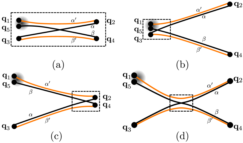
Figure 1: Trajectory configurations representing interfering mean-field solutions that dominantly contribute to the OTOC $C(t)$, Eq. (7). The trajectory quadruples reside (a) inside an encounter (marked by dashed box), form a “two-leg” diagram with an encounter (b) at the beginning or (c) at the end, or (d) build a “four-leg” diagram with the encounter in between.

Since $R_{\gamma}({\mathbf{q}}^{(\textrm{f})},{\mathbf{q}}^{(\textrm{i})};t)\!\gg\!\hbar_{\mathrm{eff}}$ in the semiclassical limit, the phase factors in Eq. (7) are generally highly oscillatory when integrating over initial or final positions. Hence, contributions from arbitrary trajectory quadruples are suppressed, while correlated quadruples with action differences such that $R_{\alpha}\!-\!R_{\alpha^{\prime}}\!+\!R_{\beta}\!-\!R_{\beta^{\prime}}\simeq\mathcal{O}(\hbar_{\mathrm{eff}})$ will dominantly contribute to $C(t)$. These are constellations where most of the time trajectories are pairwise nearly identical, except in so-called encounter regions in phase space where trajectory pairs approach each other, follow a correlated evolution and exchange their partners.

For OTOCs the relevant quadruples involve a single encounter and can be subdivided into four classes depicted in Fig. 1: Diagram (a) represents a bundle of four trajectories staying in close vicinity to each other, i.e., forming an encounter, during the whole time $t$. Panels (b) and (c) display “two-leg” diagrams with an encounter at the beginning or end, and with uncorrelated dynamics of the two trajectory pairs (“legs”) outside the encounter. The “four-leg” diagrams in (d) are characterized by uncorrelated motion before and after the encounter. The structure of the OTOC implies that the two legs on the same side of an encounter are of equal length.

Inside an encounter (boxes in Fig. 1) the hyperbolic dynamics essentially follows a common mean-field solution, i.e., linearization around one reference trajectory allows for expressing the remaining three trajectories. If their action differences are of order $\hbar_{\mathrm{eff}}$ the time scale related to an encounter just corresponds to ${\tau_{\mathrm{E}}}$ [Eqs. (20), (21) and (48) in Ref. Sup ]. Because of the exponential growth of distances in chaotic phase space the dynamics merges at the encounter boundary into uncorrelated time evolution of two trajectory legs [see, e.g., trajectories $\alpha$ and $\beta$ in Fig. 1 (b)]. Notably, Hamilton dynamics implies that this exponential separation along unstable manifolds in phase space is complemented by motion near stable manifolds, leading to the formation of (pairs of) exponentially close trajectories Sieber and Richter (2001). This mechanism gets quantum mechanically relevant for times beyond ${\tau_{\mathrm{E}}}$ [see, e.g., paths $\alpha^{\prime}$ and $\alpha$ or $\beta$ and $\beta^{\prime}$ in Figs. 1 (b) and (d)] and will prove crucial for semiclassically restoring unitarity and for explaining OTOC saturation.

The evaluation of Eq. (7) requires a thorough consideration of the dynamics in and around the encounter regions and the calculation of corresponding encounter integrals based on statistical averages invoking ergodic properties of chaotic systems. The detailed evaluation of the diagrams (a) to (d) in Fig. 1 as a function of ${\tau_{\mathrm{E}}}$ for $\hbar_{\mathrm{eff}}\!\ll\!1$ is provided in Supplemental material Sup . The ${\tau_{\mathrm{E}}}$ dependence of related objects has been considered for a variety of spectral, scattering, and transport properties of chaotic SP systems Adagideli (2003); Brouwer and Rahav (2006a); Jacquod and Whitney (2006); Waltner et al. (2008); Brouwer (2007); Kuipers et al. (2010). Conceptually, our derivation follows along the lines of these works , but requires the generalization to high-dimensional MB phase space. Moreover, the encounter integrals involve additional amplitudes related to the operators in the OTOC that demand special treatment, depending on whether the initial or final position quadratures are inside an encounter.

Using furthermore the $A_{\gamma}$ in Eq. (7) to convert integrations over final positions into initial momenta, the OTOC contribution from each diagram is conveniently represented as phase-space average

$$C(t)\simeq\int\textrm{d}^{n}q\int\textrm{d}^{n}p\,W(\mathbf{q},\mathbf{p})I(\mathbf{q},\mathbf{p};t)\,.$$ (9)

Here, $W(\mathbf{q},\mathbf{p})\!=\!\int\!\!\textrm{d}^{n}y/(2\pi\hbar_{\mathrm{eff}})^{n}\Psi^{*}\!\left(\mathbf{q}\!+\!\mathbf{y}/2\right)\Psi\left(\mathbf{q}\!-\!\mathbf{y}/2\right)$ $\exp[(\textrm{i}/\hbar_{\mathrm{eff}})\mathbf{y}\mathbf{p}]$ is the Wigner function Ozorio de Almeida (1990) of the initial state $\Psi$, and $I(\mathbf{q},\mathbf{p};t)$ comprises all encounter integrals. As shown in Ref. Sup and sketched in Fig. 2, for times $t\!<\!{\tau_{\mathrm{E}}}$ the only non-negligible contribution $I_{<}$ originates from diagram (a), whereas a combination of diagrams (c) and (d) yields the contribution $I_{>}$ nonvanishing for $t\!>\!{\tau_{\mathrm{E}}}$.

Using ${\mathbf{x}}^{(\textrm{f})}(\mathbf{x};t)$ as the final phase space point of a trajectory originating from $\mathbf{x}=(\mathbf{q},\mathbf{p})$, these terms read

$$I_{<}(\mathbf{x};t)\! =\!F_{<}\!\left(t\right)\!\left(\sum_{l=1}^{n-2}\!\!\left[{\mathbf{e}_{\textrm{s}}^{(l)}\!(\mathbf{x})}\right]_{p_{i}}\!\!\left[{\mathbf{e}_{\textrm{u}}^{(l)}\!({\mathbf{x}}^{(\textrm{f})}(\mathbf{x};t))}\right]_{q_{j}}\!\!\right)^{2}\!\!\!,$$ (10)

$$\!I_{>}(\mathbf{x};t) =F_{>}(t)\braket{\left(p_{i}-p^{\prime}_{i}\right)^{2}}_{\mathbf{x}}\left(\braket{{q^{\prime}_{j}}^{2}}_{\mathbf{x}}-\braket{q^{\prime}_{j}}_{\mathbf{x}}^{2}\right)\,.$$ (11)

Here $\braket{f(\mathbf{x}^{\prime})}_{\mathbf{x}}$ denotes the average of a phase-space function $f$ over the manifold defined through $\mathbf{x}$ by constant energy and particle density [Eq. (35) in Ref. Sup ]. In Eq. (10) the vectors $\mathbf{e}_{s/u}^{(l)}(\mathbf{x})$ denote the $n\!-\!2$ directions towards the stable, respectively unstable manifolds at $\mathbf{x}$, and the labels $q_{j}$, $p_{i}$ indicate components of those. Finally, in Eqs. (10, 11)

$$F_{<}(t) =\textrm{e}^{2\lambda(t-{\tau_{\mathrm{E}}})}\left(\frac{2}{\pi}\right)^{n-2}\left[\operatorname{Si}\left(\textrm{e}^{\lambda({\tau_{\mathrm{E}}}-t)}\right)\right]^{n-4}$$

$$\quad\times\left[\operatorname{Si}\left(\textrm{e}^{\lambda({\tau_{\mathrm{E}}}-t)}\right)-\sin\left(\textrm{e}^{\lambda({\tau_{\mathrm{E}}}-t)}\right)\right]^{2}\,,$$ (12)

$$F_{>}(t) =\left[\frac{2}{\pi}\operatorname{Si}\left(\textrm{e}^{\lambda{\tau_{\mathrm{E}}}}\right)\right]^{n-2}-\left[\frac{2}{\pi}\operatorname{Si}\left(\textrm{e}^{\lambda({\tau_{\mathrm{E}}}-t)}\right)\right]^{n-2}$$ (13)

with $\operatorname{Si}(z)\!=\!\int_{0}^{z}(\sin(z^{\prime})/z^{\prime})\textrm{d}z^{\prime}$. In the semiclassical limit follows $\lambda{\tau_{\mathrm{E}}}\!=\!\log(1/\hbar_{\mathrm{eff}})\!\gg\!1$ such that $F_{<}(t\!>\!{\tau_{\mathrm{E}}})$ is strongly suppressed (reflecting the vanishing phase space volume of quadruples of trajectories remaining close to each other over longer times) and can be expressed by a Heaviside step function,

$$F_{<}(t)\approx\textrm{e}^{2\lambda(t-{\tau_{\mathrm{E}}})}\Theta({\tau_{\mathrm{E}}}-t)=\hbar_{\mathrm{eff}}^{2}\textrm{e}^{2\lambda t}\Theta({\tau_{\mathrm{E}}}-t)\,.$$ (14)

As a result the contribution to $C(t)$ in Eq. (9), associated with $I_{<}$ and $F_{<}(t)$, is responsible for the initial exponential growth $\exp[2\lambda(t-{\tau_{\mathrm{E}}})]$ of the OTOC for $t\!<\!{\tau_{\mathrm{E}}}$, as also depicted in Fig. 2. It reflects unstable mean-field behavior.

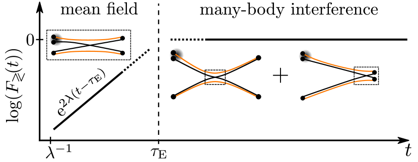
Figure 2: Universal contributions to the time evolution of the OTOC $C(t)$ for classically chaotic many-body quantum systems before [$F_{<}(t)$, Eq. (14)] and after [$F_{>}(t)$, Eq. (16)] the Ehrenfest time ${\tau_{\mathrm{E}}}\!=\!(1/\lambda)\log(N)$ marked by the vertical dashed line. The insets show diagrams (a), (d), and (c) from Fig. 1, representing interfering mean-field solutions. Not shown is the crossover regime at $t\approx{\tau_{\mathrm{E}}}$ to which all diagrams from Fig. 1 contribute.

Note that for $t\!>\!\lambda^{-1}$ (the ergodic time) Gaspard (1998)

$$\frac{\partial{q}^{(\textrm{f})}_{j}}{\partial{q}^{(\textrm{i})}_{i}}(\mathbf{x};t)\approx\!\sum_{l=1}^{n-2}\left[{\mathbf{e}_{\textrm{s}}^{(l)}\!(\mathbf{x})}\right]_{p_{i}}\!\left[{\mathbf{e}_{\textrm{u}}^{(l)}\!({\mathbf{x}}^{(\textrm{f})}(\mathbf{x};t))}\right]_{q_{j}}\!\textrm{e}^{\lambda t}\,,$$ (15)

implying that our result, Eq. (10), reduces to the short-time limit, Eq. (2), of the commutator, but moreover additionally contains the missing cutoff through $\theta({\tau_{\mathrm{E}}}-t)$.

On the contrary, $F_{>}(t)$ in Eq. (13) is suppressed for $t\!<\!{\tau_{\mathrm{E}}}$, but is indeed responsible for post-Ehrenfest OTOC saturation, as for $\lambda{\tau_{\mathrm{E}}}\!\gg\!1$ it can be approximated by

$$F_{>}(t)\approx\Theta(t-{\tau_{\mathrm{E}}})\,.$$ (16)

The underlying diagrams (c) and (d) represent dynamics swapping forth and back along distinctly different encounter-coupled mean-field solutions. This mechanism that emerges evidently in a regime where mean-field approaches fail Han and Wu (2016) creates quantum correlations and entanglement, respectively. The underlying MB interference, accounted for in the encounter integrals, is at the heart of $F_{>}(t)$ entering $I_{>}(\mathbf{x};t)$ in Eq. (11).

The latter further contains classical quantities that determine its saturation value: the variance of the $j$th final position quadrature $(\Delta q^{\prime}_{j})^{2}\!=\!\braket{{q^{\prime}_{j}}^{2}}_{\mathbf{x}}\!-\!\braket{{q^{\prime}_{j}}}_{\mathbf{x}}^{2}$ and $\braket{(p_{i}\!-\!p^{\prime}_{i})^{2}}_{\mathbf{x}}$. A straightforward calculation of the ergodic averages, exploiting the connection between ${p^{\prime}_{i}}^{2}$ and ${q^{\prime}_{j}}^{2}$ with the particle density [see Eq. (18) in Ref. Sup ] yields $I_{>}(\mathbf{x};t)\approx\theta(t-{\tau_{\mathrm{E}}})(p_{i}^{2}+1/n)\!\times\!(1/n)$.

For an initial state $\ket{\Psi}$ with a Wigner function sharply localized in phase space, the average Eq. (9) then gives

$$C(t)\approx\frac{2}{n^{2}}\textrm{ for }t>{\tau_{\mathrm{E}}}\,,$$ (17)

with corrections of $\mathcal{O}(\hbar_{\mathrm{eff}})$ due to the finite width. Interestingly, the same result, Eq. (17), holds if $\ket{\Psi}$ is an extended chaotic MB state with fixed energy and particle density.

We finally discuss several implications and conclusions:

(i) Generalization to OTOCs with other operators.–The entire line of reasoning can be generalized to OTOCs involving operators that are smooth functions of position and momentum quadratures for which a corresponding classical symbol exists Sup .

(ii) Time-reversal (TR) invariance and higher-order quantum corrections.–Remarkably, the leading quantum correction [Fig. 1(d)] is of the same order as the classical mean-field contribution at ${\tau_{\mathrm{E}}}$. Moreover, the absence of trajectory loops in the diagrams in Fig. 1, usually associated with weak localization-like corrections, implies that our results hold true for systems with and without TR symmetry. Diagrams involving more than one trajectory encounter generally yield further subleading contributions that can be susceptible to TR symmetry breaking. Their evaluation for OTOCs requires further research.

(iii) Small-$\hbar$ limit and SP systems.–Our semiclassical calculation of OTOCs in the large-$N$ limit can be readily generalized to systems of $N$ particles in $d$ spatial dimensions in the complementary limit of small $\hbar$, including the quantum chaotic SP case $N\!=\!1$. There, $\hbar_{\mathrm{eff}}\!=\!\hbar/S\!\sim\!\lambda_{\rm dB}/L$ where $\lambda_{\mathrm{dB}}$ is the de Broglie wavelength, and $S$ and $L$ are typical actions and length scales of the chaotic classical limit. Invoking the Gutzwiller propagator Gutzwiller (1991) in $n=d\cdot N$ dimensions in Eq. (5) the exponential increase of the OTOC $C_{N}(t)$ is then determined by the leading Lyapunov exponent $\lambda_{N}$ of the corresponding classical $N$-particle system (see, e.g., Refs. Kurchan (2018); Rozenbaum et al. (2017) for $N\!=\!1$). Our derivation shows that saturation sets in at the corresponding Ehrenfest time ${\tau_{\mathrm{E}}}^{(N)}\!\sim\!(1/\lambda_{N})\log(\hbar_{\mathrm{eff}}^{-1})$. We can again evaluate $C_{N}(t)$ for $t>{\tau_{\mathrm{E}}}^{(N)}$. For example, for chaotic billiards $\braket{(p_{i}-p_{i}^{\prime})^{2}}\!=\!p_{i}^{2}\!+\!p^{2}/n$. Since $L$ corresponds to the overall system size $\cal{L}$, $(\Delta q^{\prime}_{j})^{2}\!\propto\!(\mathcal{L})^{2}\!=\!L^{2}$. Thus $C_{N}(t)\!\propto\!S^{2}/n$, where the typical action $S\!=\!\hbar/\hbar_{\mathrm{eff}}$ arises here since $[\hat{q}_{j},\hat{p}_{i}]\!=\!\textrm{i}\delta_{ij}\hbar\!=\!\textrm{i}\delta_{ij}S\hbar_{\mathrm{eff}}$. Within this line of reasoning, one can view Ref. Rozenbaum et al. (2017) as a quantitative numerical confirmation of our semiclassical findings.

Interestingly, for many systems we can have $L\ll\cal{L}$, such as for the famous Lorentz gas Gaspard (1998). It is composed of scattering disks or spheres for $d\!=\!2$ or 3  with diameters setting the scale $L$. Then the dynamics is hyperbolic up to ${\tau_{\mathrm{E}}}^{(1)}$ before it becomes diffusive. This implies that $(\Delta q^{\prime}_{j})^{2}$ in Eq. (11) scales linearly with time, $(\Delta q^{\prime}_{j})^{2}\sim Dt$, with diffusion constant $D$. Thus, beyond $\tau_{E}^{(1)}$ we expect $C_{1}(t)$ to first linearly increase before it saturates at the ergodic (Thouless) time ${\cal{L}}^{2}/D$. In SP systems with diffusive dynamics arising from quantum scattering at impurities, the transport time $t_{\mathrm{tr}}$ takes the role of $\tau_{E}^{(1)}$. This implies a sharp increase of $C_{1}(t)$ for $t<t_{\mathrm{tr}}$, as already predicted in Ref. Larkin and Ovchinnikov (1969), followed by the diffusive behavior discussed above.

(iv) Nonergodic many-body dynamics.–The nonlinear mean-field dynamics associated with the classical limit of MB Fock space is much less understood Borgonovi et al. (2018); Tomsovic et al. (2018); Tomsovic (2018) than its SP counterpart. If the MB dynamics is diffusive for $t\!>\!{\tau_{\mathrm{E}}}$, we expect a similar time dependence for $C(t)$ as discussed in (iii). The propagator Eq. (5) is not restricted to chaotic dynamics, but also allows for investigating the imprint of more complex, e.g., mixed regular-chaotic, phase space dynamics on OTOCs or, more generally, on the stability of MB quantum evolution per se.

To conclude, we considered the time evolution of OTOCs by developing a general semiclassical approach for interacting large-$N$ systems. It links chaotic motion in the classical mean-field limit to the correlated quantum many-body dynamics in terms of interference between mean-field solutions giving rise to scrambling and entanglement. We uncovered the relevant many-body quantum interference mechanism that is responsible for the commonly observed saturation of OTOCs at the scrambling or Ehrenfest time. While we explicitly derived OTOCs for bosonic systems, similar considerations should be possible for fermionic many-body systems posing an interesting problem for future research.

Supplemental material to the paper
“Many-Body Quantum Interference and the Saturation
of Out-of-Time-Order Correlators”

Here we provide detailed calculations of the contributions of the diagram classes (a) to (d) (in Fig. 1 of the main text) to the out-of-time-order correlator (OTOC).

I Phase space structure of the classical limit of the generalized Bose-Hubbard system

The classical limit of the Bose-Hubbard model described by Hamiltonian (3) of the main text is found to be $\mathcal{H}^{\mathrm{cl}}$ given in Eq. (6). Generically, this Hamiltonian has at least two constants of motion (CoM), the energy, represented by the value of $\mathcal{H}^{\mathrm{cl}}$, and the conservation of particle density, represented by

$$\mathcal{N}(\mathbf{q},\mathbf{p})=\sum_{i=1}^{n}|\Phi_{i}|^{2}=\frac{1}{2}\sum_{i=1}^{n}\left(q_{i}^{2}+p_{i}^{2}\right)\,.$$ (18)

We assume that the system does not have any other CoMs and displays fully chaotic motion on the $(2n-2)$-dimensional submanifold defined by the CoMs. Locally at any phase-space (PS) point $\mathbf{x}=(\mathbf{q},\mathbf{p})$, the coordinate system of the tangent space can be defined in such a way that for each CoM one can associate 2 axes (parallel and perpendicular to the flow defined by them), and the remaining $2(n-2)$ axis point along the stable or unstable directions responsible for the fully hyperbolic dynamics, see e.g. Gaspard (1998). In the following, we denote the latter directions with ${\mathbf{e}_{\textrm{s}}^{(l)}\!(\mathbf{x})}$, ${\mathbf{e}_{\textrm{u}}^{(l)}\!(\mathbf{x})}$, $l\!=\!1,\ldots n-2$. Physically, if the difference of the initial conditions of two trajectories lies in the direction ${\mathbf{e}_{\textrm{s}}^{(l)}\!(\mathbf{x})}$ $({\mathbf{e}_{\textrm{u}}^{(l)}\!(\mathbf{x})})$, the hyperbolic dynamics of the chaotic system will exponentially increase (decrease) this difference, with a rate given by the associated classical Lyapunov exponent $\lambda_{l}$. For simplicity, we will assume that the chaotic dynamics is uniformly hyperbolic, i.e. all stable and unstable directions share the same Lyapunov exponent $\lambda$. A discussion of the generic hyperbolic case would only lead to a significant increase of the complexity of the calculations, while the result remains the same in the two limits $t\ll{\tau_{\mathrm{E}}}$ and $t\gg{\tau_{\mathrm{E}}}$.

II Geometry of encounters in phase space

For our calculations it is necessary to understand how to quantify constellations of two trajectories which encounter each other in a PS region, as displayed in Fig. 1. For a detailed analysis of the single-particle case, there is a broad literature available Müller et al. (2007, 2005); Waltner et al. (2008); Turek and Richter (2003); Spehner (2003). For the ease of the reader, and also to be able to explain some OTOC-related special aspects in the next section, we summarize the key steps here.

The main idea is that during an encounter of two trajectories in PS the dynamics of their relative motion is well described by linearizing Hamilton’s equations of motion around one of the trajectories. In this linearized regime, the relative difference of the trajectories in PS can be expressed in the local coordinate system spanned by the directions towards the stable and unstable manifolds, as well as the manifolds given by the CoMs, see the previous section. However, we have to demand that both trajectories have (within a window of $\mathcal{O}(\hbar_{\mathrm{eff}})$) the same values for their CoMs, since later we will construct partner trajectories partially following both trajectories. Thus, the relative difference vector is expressed solely in terms of the $2(n\!-\!2)$ stable and unstable directions.

To quantitatively describe two trajectories $\alpha$, $\beta$ encountering each other in PS, we first choose one of the trajectories as a reference trajectory, say $\beta$, and then take a time $t^{\prime}$ at which we assume $\beta$ to be close to $\alpha$. At the PS point of $\beta$ at $t^{\prime}$, denoted by $\mathbf{x}_{\beta}(t^{\prime})$, we place the origin of a $2(n\!-\!2)$ dimensional coordinate system, which is spanned by the local stable and unstable directions ${\mathbf{e}_{\beta,\textrm{s}}^{(l)}\!(t^{\prime})}\!\equiv\!{\mathbf{e}_{\textrm{s}}^{(l)}\!(\mathbf{x}_{\beta}(t^{\prime}))}$, ${\mathbf{e}_{\beta,\textrm{u}}^{(l)}\!(t^{\prime})}\!\equiv\!{\mathbf{e}_{\textrm{u}}^{(l)}\!(\mathbf{x}_{\beta}(t^{\prime}))}$. In this frame, an encountering trajectory $\alpha$, which takes the same values of the CoMs as $\beta$, is uniquely defined by vectors $\mathbf{s}$, $\mathbf{u}$, as

$$\mathbf{x}_{\alpha}(t^{\prime})=\mathbf{x}_{\beta}(t^{\prime})+\sum_{l=1}^{n-2}\left[s_{l}{\mathbf{e}_{\beta,\textrm{s}}^{(l)}\!(t^{\prime})}+u_{l}{\mathbf{e}_{\beta,\textrm{u}}^{(l)}\!(t^{\prime})}\right]\vspace{-2ex}$$ (19)

uniquely defines the trajectory’s PS point at time $t^{\prime}$. In the linearizable regime of the relative Hamiltonian dynamics, i.e. as long as the components of the vectors $\mathbf{s}$, $\mathbf{u}$ do not reach a given critical (classical) value $\pm c$, this single PS point is well defined and, for a time-independent Hamilton function, is sufficient to define the trajectory $\alpha$. In the main text, this cutoff $c$ has been set to $1$ for the ease of readability. The only assumption is that $c^{2}$ is a typical classical action scale, i.e. large compared to $\hbar_{\mathrm{eff}}$. Its exact value is not of importance as diagrams with action differences much larger than $\hbar_{\mathrm{eff}}$ do not contribute to the results of semiclassical calculations, and reliable quantitative results do not depend on it.

Note that in Eq. (19) the temporal parametrization of $\alpha$ is such, that $\alpha$ enters the encounter region simultaneously with $\beta$. As seen from Eq. (7), $\alpha$ and $\beta$ need the same time to get from the initial to the final point. A mismatch in times of the encounter event of the trajectories $\alpha$ and $\beta$ would lead to partner trajectories $\alpha^{\prime}$, $\beta^{\prime}$ with times different to $t$. But those are not available in the sums over trajectories $\alpha^{\prime}$, $\beta^{\prime}$ in Eq. (7).

Subject to the hyperbolic dynamics, the vectors $\mathbf{s}$ and $\mathbf{u}$ in the co-traveling coordinate system will change when varying $t^{\prime}$. For instance for $t^{\prime}$, $t^{\prime\prime}$ inside the encounter, the PS points given by $\left(t^{\prime},\mathbf{s},\mathbf{u}\right)$ and $(t^{\prime\prime},\mathbf{s}\exp[-\lambda(t^{\prime\prime}\!-\!t^{\prime})],\mathbf{u}\exp[\lambda(t^{\prime\prime}\!-\!t^{\prime})])$ are describing the very same trajectory $\alpha$. To avoid overcounting, it is necessary to later divide the contributions by the time the trajectories spend inside the encounter region. The limits of the encounter regions are reached, when the first components of $\mathbf{s}$ and $\mathbf{u}$ have grown to a classical scale $\pm c$ at which the linearization breaks down. This introduces two time scales,

$$\begin{aligned} t_{\textrm{s}}(\mathbf{s})&=\frac{1}{\lambda}\log\left(\frac{c}{\max_{i=1,\ldots,n-2}(|s_{i}|)}\right)\,,\\ t_{\textrm{u}}(\mathbf{u})&=\frac{1}{\lambda}\log\left(\frac{c}{\max_{i=1,\ldots,n-2}(|u_{i}|)}\right)\,,\end{aligned}$$ (20)

and the time for a fully developed encounter, as seen in Fig. 1 (d), is defined as the sum

$$t_{\mathrm{enc}}\left(\mathbf{s},\mathbf{u}\right)=t_{\textrm{s}}(\mathbf{s})+t_{\textrm{u}}(\mathbf{u})\,.$$ (21)

Note that if the trajectories start and/or end inside the encounter region, as in Fig. 1 (a) to (c), the encounter time has to be reduced accordingly.

Suitable partner trajectories following the original trajectories outside the encounter region, while interchanging partners inside it, are found by the PS points

$$\begin{aligned} \mathbf{x}_{\beta^{\prime}}(t^{\prime})&=\mathbf{x}_{\beta}(t^{\prime})+\sum_{l=1}^{n-2}s_{l}{\mathbf{e}_{\beta,\textrm{s}}^{(l)}\!(t^{\prime})}\,,\\ \mathbf{x}_{\alpha^{\prime}}(t^{\prime})&=\mathbf{x}_{\beta}(t^{\prime})+\sum_{l=1}^{n-2}u_{l}{\mathbf{e}_{\beta,\textrm{u}}^{(l)}\!(t^{\prime})}\,.\end{aligned}$$ (22)

According to their definition, trajectory $\beta^{\prime}$ exponentially approaches $\beta$ for times larger than $t^{\prime}$, as their difference is solely along stable directions. For times smaller than $t^{\prime}$, we have to consider time-reversed dynamics, and the stable and unstable manifolds interchange their roles. Thus, for times smaller than $t^{\prime}$, $\beta^{\prime}$ exponentially separates from $\beta$, and exponentially approaches $\alpha$ in the same fashion, since

$$\mathbf{x}_{\alpha}(t^{\prime})-\mathbf{x}_{\beta^{\prime}}(t^{\prime})=\sum_{l=1}^{n-2}u_{l}{\mathbf{e}_{\beta,\textrm{u}}^{(l)}\!(t^{\prime})}.$$ (23)

The same reasoning can be applied to $\alpha^{\prime}$.

To summarize, a constellation of trajectories with a single encounter is described by choosing one of the trajectories as a reference trajectory, a time $t^{\prime}$ as time of the encounter, and vectors $\mathbf{s}$, $\mathbf{u}$ to quantify the respective distances towards the other trajectories.

Regarding encounter contributions to OTOCs, there is a further subtlety to consider. If the initial points of the trajectories are contained inside the encounter region, we have to treat classical quantities related to initial points of trajectories in a correlated way, and also use the local coordinates $\mathbf{s}$, $\mathbf{u}$ to describe them. In Fig. 1 (a) and (b), the beginning of the trajectories is inside the encounter region. This requires to treat the difference of initial momenta in Eq. (7) through

$$\begin{aligned} {p}^{(\textrm{i})}_{\alpha^{\prime},i}-{p}^{(\textrm{i})}_{\alpha,i}&=-\sum_{l=1}^{n-2}s_{l}\textrm{e}^{\lambda t^{\prime}}\left[{\mathbf{e}_{\beta,\textrm{s}}^{(l)}\!(0)}\right]_{p_{i}},\\ {p}^{(\textrm{i})}_{\beta,i}-{p}^{(\textrm{i})}_{\beta^{\prime},i}&=-\sum_{l=1}^{n-2}s_{l}\textrm{e}^{\lambda t^{\prime}}\left[{\mathbf{e}_{\beta,\textrm{s}}^{(l)}\!(0)}\right]_{p_{i}}.\end{aligned}$$ (24)

Similarly, if the final points enter the encounter region, as in Fig. 1 (a) and (c), we use

$${q}^{(\textrm{f})}_{\alpha,j}{q}^{(\textrm{f})}_{\beta,j}=\frac{1}{2}\left({{q}^{(\textrm{f})}_{\alpha,j}}^{2}+{{q}^{(\textrm{f})}_{\beta,j}}^{2}\right)-\frac{1}{2}\left({q}^{(\textrm{f})}_{\alpha,j}-{q}^{(\textrm{f})}_{\beta,j}\right)^{2}$$

$$\approx{{q}^{(\textrm{f})}_{\alpha,j}}^{2}-\frac{1}{2}\left(\sum_{l=1}^{n-2}u_{l}\textrm{e}^{\lambda(t-t^{\prime})}\left[{\mathbf{e}_{\beta,\textrm{u}}^{(l)}\!(t)}\right]_{q_{j}}\right)^{2}.$$ (25)

Here $\left[.\right]_{p_{i}}$ and $\left[.\right]_{q_{j}}$ denote the $i$-th component of the momentum sector, and the $j$-th component of the coordinate sector of the PS vector ${\mathbf{e}_{\beta,\textrm{u}}^{(l)}\!(t)}$. As we will later approximate the square of the final points in Eq. (25) by its ergodic average, we already approximate them here by ${{q}^{(\textrm{f})}_{\alpha,j}}^{2}$ to simplify the expressions.

III Density and action difference of diagrams with encounters

To obtain all possible contributions to Eq. (7) from trajectory constellations with an encounter, we first introduce integrations over the relative differences $\mathbf{s}$, $\mathbf{u}$ and time $t^{\prime}$ at which these differences are employed. The four-fold sum over trajectories is then reduced to a two-fold sum, as the partner trajectories $\alpha^{\prime}$ and $\beta^{\prime}$ are uniquely given by the Eqs. (22). Furthermore, we correlate the remaining sums over $\alpha$ and $\beta$ by introducing the density distribution

$$\rho_{\alpha,\beta}\left(\mathbf{s},\mathbf{u},t^{\prime}\right)=\frac{(2\pi\hbar_{\mathrm{eff}})^{2}}{t_{\mathrm{enc}}\left(\mathbf{s},\mathbf{u}\right)}\delta^{2n}\left[\mathbf{x}_{\alpha}(t^{\prime})-\tilde{\mathbf{x}}\left(\mathbf{x}_{\beta}(t^{\prime}),\mathbf{s},\mathbf{u}\right)\right],$$ (26)

where

$$\tilde{\mathbf{x}}\left(\mathbf{x},\mathbf{s},\mathbf{u}\right)=\mathbf{x}+\sum_{l=1}^{n-2}\left[s_{l}{\mathbf{e}_{\textrm{s}}^{(l)}\!(\mathbf{x})}+u_{l}{\mathbf{e}_{\textrm{u}}^{(l)}\!(\mathbf{x})}\right]\,.$$ (27)

The normalization $(2\pi\hbar_{\mathrm{eff}})^{2}$ in Eq. (26) is independently determined by performing subsequent calculations imposing unitarity for the object $1\!=\!\braket{\Psi}{\hat{U}^{\dagger}(t)\hat{U}(t)\hat{U}^{\dagger}(t)\hat{U}(t)}{\Psi}$. It reflects that the paired trajectories should all stay in the window of a Planck cell near the submanifold defined by the reference trajectory’s values for the CoMs energy and particle density.

The action difference of this system of four trajectories is found to be Turek and Richter (2003); Müller et al. (2005)

$$R_{\alpha}-R_{\alpha^{\prime}}+R_{\beta}-R_{\beta^{\prime}}\approx\mathbf{s}\cdot\mathbf{u}+{\mathbf{p}}^{(\textrm{i})}_{\alpha}(\mathbf{q}_{1}-\mathbf{q}_{5}),$$ (28)

where the latter term related to the initial momentum and the relative distance $\mathbf{y}\!=\!\mathbf{q}_{1}\!-\!\mathbf{q}_{5}$ is introduced as we substitute the trajectories $\alpha$, $\alpha^{\prime}$, starting at $\mathbf{q}_{1}$ and $\mathbf{q}_{5}$, by nearby trajectories starting at $\mathbf{q}\!=\!\frac{1}{2}(\mathbf{q}_{1}\!+\!\mathbf{q}_{5})$.

IV Contributions of encounter diagrams to the OTOC

IV.1 Contributions of 4-leg-encounters

We start with the contributions of the 4-leg-encounters displayed in Fig. 1 (d). This term is given by

$$C^{(\mathrm{4le})}(t) =\int\textrm{d}^{n}q\!\int\textrm{d}^{n}y\!\int\textrm{d}^{n}q_{2}\!\int\textrm{d}^{n}q_{3}\!\int\textrm{d}^{n}q_{4}\,\Psi^{*}\left(\mathbf{q}+\frac{\mathbf{y}}{2}\right)\Psi\left(\mathbf{q}-\frac{\mathbf{y}}{2}\right)\sum_{\begin{subarray}{c}\alpha:\mathbf{q}_{3}\overset{t}{\rightarrow}\mathbf{q}_{2}\\ \beta:\mathbf{q}\rightarrow\mathbf{q}_{4}\end{subarray}}|A_{\alpha}|^{2}|A_{\beta}|^{2}\left({p}^{(\textrm{i})}_{\beta,i}-{p}^{(\textrm{i})}_{\alpha,i}\right)^{2}{q}^{(\textrm{f})}_{\alpha,j}{q}^{(\textrm{f})}_{\beta,j}\textrm{e}^{\frac{\textrm{i}}{\hbar_{\mathrm{eff}}}{\mathbf{p}}^{(\textrm{i})}_{\alpha}\mathbf{y}}$$

$$\qquad\times\int_{-c}^{c}\textrm{d}^{n-2}s\int_{-c}^{c}\textrm{d}^{n-2}u\int_{t_{\textrm{s}}(\mathbf{s})}^{t-t_{\textrm{u}}(\mathbf{u})}\textrm{d}t^{\prime}\textrm{e}^{\frac{\textrm{i}}{\hbar_{\mathrm{eff}}}\mathbf{s}\mathbf{u}}\Theta\left[t-t_{\mathrm{enc}}(\mathbf{s},\mathbf{u})\right]\rho_{\alpha,\beta}\left(\mathbf{s},\mathbf{u},t^{\prime}\right).$$ (29)

Most of the ingredients for this integral have been already discussed in the previous two sections. The special features of Fig. 1 (d) are represented by the boundaries of the integration over $t^{\prime}$, which require that the encounter region does neither contain the beginning nor the end of the trajectories. The Heaviside step function $\Theta$ finally ensures that encounter regions longer than the available time $t$ are excluded.

In a first step we use the fact that the squared amplitudes $|A_{\alpha}|^{2}$ can be interpreted as Jacobian for a variable transformation from final coordinates to initial momenta along a classical trajectory,

$$|A_{\alpha}|^{2}=\frac{1}{(2\pi\hbar_{\mathrm{eff}})^{n}}\left|\frac{\partial{\mathbf{p}}^{(\textrm{i})}_{\alpha}}{\partial{\mathbf{q}}^{(\textrm{f})}}\right|\,.$$ (30)

Together with the sum over trajectories $\alpha$, we can transform the integrations over $\mathbf{q}_{2}\!=\!{\mathbf{q}}^{(\textrm{f})}_{\alpha}$ to an integration over initial momenta $\mathbf{p}_{3}$. Trajectory-related quantities labeled by $\alpha$ become then functions of trajectories with initial conditions $\mathbf{x}_{3}\!=\!(\mathbf{q}_{3},\mathbf{p}_{3})$, e.g.

$$\left({\mathbf{p}}^{(\textrm{i})}_{\alpha},{\mathbf{q}}^{(\textrm{f})}_{\alpha}\right)\to\left(\mathbf{p}_{3},{\mathbf{q}}^{(\textrm{f})}\left(\mathbf{q}_{3},\mathbf{p}_{3};t\right)\right)\,.$$ (31)

In the same spirit we use the sum over $\beta$ with $|A_{\beta}|^{2}$ to transform the integration over $\mathbf{q}_{4}$ to $\mathbf{p}$, and $\beta$-labeled quantities become functions of $\mathbf{x}\!=\!(\mathbf{q},\mathbf{p})$.

The $\delta$-function in the density of encounters (26) can be interpreted as classical probability density for a trajectory starting at $(\mathbf{q}_{3},\mathbf{p}_{3})$ to be at time $t^{\prime}$ at a certain phase space point which depends on $\mathbf{q}$, $\mathbf{p}$, $\mathbf{s}$, $\mathbf{u}$ and $t^{\prime}$. As the initial points $(\mathbf{q}_{3},\mathbf{p}_{3})$ are not located within the encounter region, it is justified to utilize the ergodic property of the chaotic system, which states that every accessible PS point is equally likely to be reached by the classical dynamics. We can thus approximate $\rho_{\alpha,\beta}$ by

$$\rho_{\alpha,\beta}\to\frac{(2\pi\hbar_{\mathrm{eff}})^{2}}{t_{\mathrm{enc}}\left(\mathbf{s},\mathbf{u}\right)}\frac{\delta^{2}\begin{pmatrix}\mathcal{H}^{\textrm{cl}}(\mathbf{x}_{3})-\mathcal{H}^{\textrm{cl}}(\mathbf{x})\\ \mathcal{N}(\mathbf{x}_{3})-\mathcal{N}(\mathbf{x})\end{pmatrix}}{\Sigma(\mathbf{x})}\,,$$ (32)

where $\Sigma(\mathbf{x})$ is the volume of the chaotic PS submanifold,

$$\Sigma(\mathbf{x})=\int d^{2n}\!x^{\prime}\,\delta^{2}\begin{pmatrix}\mathcal{H}^{\textrm{cl}}(\mathbf{x}^{\prime})-\mathcal{H}^{\textrm{cl}}(\mathbf{x})\\ \mathcal{N}(\mathbf{x}^{\prime})-\mathcal{N}(\mathbf{x})\end{pmatrix}\,.$$ (33)

Together with the integration over initial PS points $\mathbf{x}_{3}$, ergodic PS averages are introduced, which lead to the following substitution of initial momenta and final position:

$$\left(p_{3,i}-p_{i}\right)^{2}{q}^{(\textrm{f})}_{j}\!\left(\mathbf{x}_{3};t\right)\to\Braket{\left(p^{\prime}_{i}-p_{i}\right)^{2}{q}^{(\textrm{f})}_{j}\!\left(\mathbf{x}^{\prime};t\right)}_{\mathbf{x}}\,,$$ (34)

where the ergodic PS average is defined as

$$\Braket{f(\mathbf{x}^{\prime})}_{\mathbf{x}}=\frac{\int d^{2n}\!x^{\prime}\,\delta^{2}\begin{pmatrix}\mathcal{H}^{\textrm{cl}}(\mathbf{x}^{\prime})-\mathcal{H}^{\textrm{cl}}(\mathbf{x})\\ \mathcal{N}(\mathbf{x}^{\prime})-\mathcal{N}(\mathbf{x})\end{pmatrix}f(\mathbf{x}^{\prime})}{\Sigma(\mathbf{x})}\,.$$ (35)

For times longer than the ergodic time $\lambda^{-1}$ we can further assume that the final position is independent of its starting point, and the average factorizes,

$$\Braket{\left(p^{\prime}_{i}-p_{i}\right)^{2}{q}^{(\textrm{f})}_{j}\!\left(\mathbf{x}^{\prime};t\right)}_{\mathbf{x}}=\Braket{\left(p^{\prime}_{i}-p_{i}\right)^{2}}_{\mathbf{x}}\Braket{q^{\prime}_{j}}_{\mathbf{x}}\,.$$ (36)

With the same reasoning, we can also approximate the remaining factor ${q}^{(\textrm{f})}_{j}\!\left(\mathbf{x};t\right)$ by its ergodic average $\braket{q^{\prime}_{j}}_{\mathbf{x}}$. After introducing the Wigner function,

$$W(\mathbf{q},\mathbf{p})\!=\!\int\!\frac{\textrm{d}^{n}y}{(2\pi\hbar_{\mathrm{eff}})^{n}}\Psi^{*}\left(\mathbf{q}+\frac{\mathbf{y}}{2}\right)\Psi\left(\mathbf{q}-\frac{\mathbf{y}}{2}\right)\textrm{e}^{\frac{\textrm{i}}{\hbar_{\mathrm{eff}}}\mathbf{p}\mathbf{y}}\,,$$ (37)

we see that the contribution of four-leg encounters can be written in terms of a PS average weighted with the Wigner function,

$$C^{(\mathrm{4le})}(t)=\int\!\textrm{d}^{n}q\!\int\!\textrm{d}^{n}p\,W\left(\mathbf{q},\mathbf{p}\right)I^{(\mathrm{4le})}\left(\mathbf{q},\mathbf{p};t\right)\,.$$ (38)

Here the PS function

$$I^{(\mathrm{4le})}\left(\mathbf{q},\mathbf{p};t\right)=\Braket{\left(p^{\prime}_{i}-p_{i}\right)^{2}}_{\mathbf{x}}\Braket{q^{\prime}_{j}}_{\mathbf{x}}^{2}F^{(\mathrm{4le})}(t)$$ (39)

contains the ergodic PS averages (36) and the encounter integral

$$F^{(\mathrm{4le})}(t) =\frac{1}{(2\pi\hbar_{\mathrm{eff}})^{n-2}}\int_{-c}^{c}\!\!\textrm{d}^{n-2}s\!\int_{-c}^{c}\!\!\textrm{d}^{n-2}u\,\textrm{e}^{\frac{\textrm{i}}{\hbar_{\mathrm{eff}}}\mathbf{s}\mathbf{u}}$$

$$\qquad\times\frac{t-t_{\mathrm{enc}}(\mathbf{s},\mathbf{u})}{t_{\mathrm{enc}}(\mathbf{s},\mathbf{u})}\Theta\left[t-t_{\mathrm{enc}}(\mathbf{s},\mathbf{u})\right]\,.$$ (40)

In order to resolve the $\max$-function in the definition of $t_{\mathrm{enc}}$, we split the integrations over $\mathbf{s}$, $\mathbf{u}$. This leads to the summation

$$F^{(\mathrm{4le})}(t)\!=\!\sum_{i,j=1}^{n-2}F^{(\mathrm{4le})}_{ij}(t)\,,$$ (41)

where

$$F^{(\mathrm{4le})}_{ij}(t) =\frac{1}{(2\pi\hbar_{\mathrm{eff}})^{n-2}}\int_{-c}^{c}\!\!\textrm{d}s_{i}\!\int_{-c}^{c}\!\!\textrm{d}u_{j}\,\frac{t-t_{\mathrm{enc}}(s_{i}u_{j})}{t_{\mathrm{enc}}(s_{i}u_{j})}\Theta\left[t-t_{\mathrm{enc}}(s_{i}u_{j})\right]\left(\prod_{\begin{subarray}{c}k,k^{\prime}=1\\ k\neq i,\,k^{\prime}\neq j\end{subarray}}^{n-2}\!\!\int_{-|s_{i}|}^{|s_{i}|}\!\!\textrm{d}s_{k}\!\int_{-|u_{j}|}^{|u_{j}|}\!\!\textrm{d}u_{k^{\prime}}\!\right)\textrm{e}^{\frac{\textrm{i}}{\hbar_{\mathrm{eff}}}\mathbf{s}\mathbf{u}}\,,$$ (42)

with the encounter time $t_{\mathrm{enc}}(s_{i}u_{j})\!=\!(1/\lambda)\log(c^{2}/|s_{i}u_{j}|)$, see Eq. (21).

One has to distinguish the cases $i\!\neq\!j$ from $i\!=\!j$ in order to correctly interpret the product over $k$, $k^{\prime}$. The integrations over $s_{k}$ and $u_{k^{\prime}}$ are easily performed, either by a simple integration of an exponential for $k\!=\!j$, $k^{\prime}\!=\!i$, $i\!\neq\!j$, or by sorting the products such that $k\!=\!k^{\prime}$ and using Eq. (97). For the integration over $s_{i}$, $u_{j}$, one first transforms the integration over the subinterval $[-c,0]$ to $[0,c]$ by inverting the sign of the integration variables. For the resulting integrations over positive $s_{i}$, $u_{j}$ we then use the variable transformation Brouwer and Rahav (2006a)

$$(s_{i},u_{j}) \to(S,\sigma)=\left(\frac{s_{i}u_{j}}{c^{2}},\frac{c}{u_{j}}\right)\textrm{, with }\left|\frac{\partial(s_{i},u_{j})}{\partial(S,\sigma)}\right|=\frac{c^{2}}{\sigma}$$

$$\quad\textrm{ and }0<S<1,\,1<\sigma<\frac{1}{S}\,.$$ (43)

The integration over $\sigma$ leads to the cancellation of $t_{\mathrm{enc}}(s_{i}u_{j})$ in the denominator. The argument of the Heaviside step function $\Theta$ demands $t\!>\!(1/\lambda)\log(S^{-1})$, which is equivalent to $S\!>\!\exp(-\lambda t)$, thus raising the lower integration limit for $S$. We get as result for $i\!=\!j$

$$F^{(\mathrm{4le})}_{ii}(t) =\left(\frac{2}{\pi}\right)^{n-2}\int_{\textrm{e}^{-\lambda t}}^{1}\textrm{d}S\left(\lambda t-\log\left(\frac{1}{S}\right)\right)$$

$$\qquad\times\operatorname{Si}^{n-3}\left(\frac{c^{2}S}{\hbar_{\mathrm{eff}}}\right)\cos\left(\frac{c^{2}S}{\hbar_{\mathrm{eff}}}\right)\frac{c^{2}}{\hbar_{\mathrm{eff}}}\,,$$ (44)

and for $i\!\neq\!j$

$$F^{(\mathrm{4le})}_{ij}(t) =\left(\frac{2}{\pi}\right)^{n-2}\int_{\textrm{e}^{-\lambda t}}^{1}\textrm{d}S\left(\lambda t-\log\left(\frac{1}{S}\right)\right)$$

$$\qquad\times\operatorname{Si}^{n-4}\left(\frac{c^{2}S}{\hbar_{\mathrm{eff}}}\right)\frac{\sin^{2}\left(\frac{c^{2}S}{\hbar_{\mathrm{eff}}}\right)}{S}\,,$$ (45)

where $\operatorname{Si}(z)=\int_{0}^{z}\textrm{d}z^{\prime}(\sin(z^{\prime})/z^{\prime})$ denotes the sine integral.

We can now perform the summation over indices $i$, $j$ to obtain an integral expression for $F^{(\mathrm{4le})}$. Note that

$$(n-2)(n-3)\operatorname{Si}^{n-4}\left(\frac{c^{2}S}{\hbar_{\mathrm{eff}}}\right)\frac{\sin^{2}\left(\frac{c^{2}S}{\hbar_{\mathrm{eff}}}\right)}{S}$$

$$\quad+(n-2)\operatorname{Si}^{n-3}\left(\frac{c^{2}S}{\hbar_{\mathrm{eff}}}\right)\cos\left(\frac{c^{2}S}{\hbar_{\mathrm{eff}}}\right)\frac{c^{2}}{\hbar_{\mathrm{eff}}}$$

$$=\frac{\textrm{d}}{\textrm{d}S}S\frac{\textrm{d}}{\textrm{d}S}\operatorname{Si}^{n-2}\left(\frac{c^{2}S}{\hbar_{\mathrm{eff}}}\right)\,,$$ (46)

and thus

$$F^{(\mathrm{4le})}(t) =\left(\frac{2}{\pi}\right)^{n-2}\int_{\textrm{e}^{-\lambda t}}^{1}\textrm{d}S\left(\lambda t-\log\left(\frac{1}{S}\right)\right)$$

$$\qquad\times\frac{\textrm{d}}{\textrm{d}S}S\frac{\textrm{d}}{\textrm{d}S}\operatorname{Si}^{n-2}\left(\frac{c^{2}S}{\hbar_{\mathrm{eff}}}\right)\,.$$ (47)

The outer derivative in the second line is shifted to the first factor in the integrand. As $\textrm{d}/\textrm{d}S\,(t\!-\!\log(S^{-1}))\!=\!1/S$ cancels the factor $S$, the remaining integral is easily performed. To obtain more physical insight at this stage, it is worth to introduce the Ehrenfest time,

$${\tau_{\mathrm{E}}}=\frac{1}{\lambda}\log\left(\frac{c^{2}}{\hbar_{\mathrm{eff}}}\right)\quad\Leftrightarrow\quad\frac{c^{2}}{\hbar_{\mathrm{eff}}}=\textrm{e}^{\lambda{\tau_{\mathrm{E}}}}\,.$$ (48)

It is the time scale for which under hyperbolic dynamics details of the order of $\hbar_{\mathrm{eff}}$ can grow to the typical classical action $c^{2}$. Using this, we obtain as final result

$$F^{(\mathrm{4le})}(t)=\left(\frac{2}{\pi}\right)^{n-2}\lambda t(n-2)\operatorname{Si}^{n-3}\left(\textrm{e}^{\lambda{\tau_{\mathrm{E}}}}\right)\sin\left(\textrm{e}^{\lambda{\tau_{\mathrm{E}}}}\right)$$

$$\quad-\left(\frac{2}{\pi}\right)^{n-2}\left[\operatorname{Si}^{n-2}\left(\textrm{e}^{\lambda{\tau_{\mathrm{E}}}}\right)-\operatorname{Si}^{n-2}\left(\textrm{e}^{\lambda\left({\tau_{\mathrm{E}}}-t\right)}\right)\right]\,.$$ (49)

In the semiclassical limit $\hbar_{\mathrm{eff}}\!\ll\!c^{2}$, ${\tau_{\mathrm{E}}}$ in Eq. (48) is large compared to the ergodic time $\lambda^{-1}$ implying a separation of time scales for the OTOC. Thus, $\exp(\lambda{\tau_{\mathrm{E}}})\!\gg\!1$, and this has several consequences:

• $\sin[\exp(\lambda{\tau_{\mathrm{E}}})]$ is highly oscillatory and can be neglected in the phase space average (38).

• $\operatorname{Si}[\exp(\lambda{\tau_{\mathrm{E}}})]$ is well approximated by the asymptotic limit of the sine integral for large, positive arguments, $\operatorname{Si}[\exp(\lambda{\tau_{\mathrm{E}}})]\!\approx\!\frac{\pi}{2}$.

• For $t<{\tau_{\mathrm{E}}}$ Taylor-expansion around $t/{\tau_{\mathrm{E}}}\!=\!0$ yields

  $$\operatorname{Si}^{n-2}\left(\textrm{e}^{\lambda{\tau_{\mathrm{E}}}}\right)-\operatorname{Si}^{n-2}\left(\textrm{e}^{\lambda({\tau_{\mathrm{E}}}-t)}\right)$$

  $$\approx(n-2)\operatorname{Si}^{n-3}\left(\textrm{e}^{\lambda{\tau_{\mathrm{E}}}}\right)\sin\left(\textrm{e}^{\lambda{\tau_{\mathrm{E}}}}\right)\lambda t\,,$$ (50)

  where the term linear in $t$ is the same highly oscillatory term as in the first item and can be neglected. (Alternatively, if not neglected, it would exactly cancel the oscillatory term for small $t$.)

• For $t\!>\!{\tau_{\mathrm{E}}}$ we have $\exp[\lambda({\tau_{\mathrm{E}}}\!-\!t)]\!\ll\!1$, and thus, by Taylor-expanding $\operatorname{Si}(y)$ around $y\!=\!0$, we get

  $$\operatorname{Si}^{n-2}\left(\textrm{e}^{\lambda({\tau_{\mathrm{E}}}-t)}\right)\approx\textrm{e}^{(n-2)\lambda({\tau_{\mathrm{E}}}-t)}\,,$$ (51)

  which is exponentially fast decaying for $t\!>\!{\tau_{\mathrm{E}}}$ and can be neglected for $t\!\gg\!{\tau_{\mathrm{E}}}$.

Combining the above considerations, we can well approximate

$$F^{\mathrm{(4le)}}(t)\approx\left\{\begin{matrix}0&\textrm{ if }t\ll{\tau_{\mathrm{E}}}\\ -1&\textrm{ if }t\gg{\tau_{\mathrm{E}}}\end{matrix}\right\}\approx-\Theta\left(t-{\tau_{\mathrm{E}}}\right)\,.$$ (52)

Hence the diagram class of the 4-leg-encounters only contributes after a certain minimal time, the Ehrenfest time ${\tau_{\mathrm{E}}}$. It is after this time that a description solely based on classical dynamics breaks down, as interference contributions due to trajectory constellations with encounter regions with an action difference of the order $\hbar_{\mathrm{eff}}$ start to exist.

IV.2 Contributions of 2-leg-encounters

2-leg encounter diagrams are characterized by an encounter region that contains either the starting or the end points of the quadruplet of trajectories, see Fig. 1 (b) and (c).

IV.2.1 Encounter at the beginning

We start with diagram (b). Its contribution $C^{\textrm{(2le,(b))}}$ is calculated from a similar expression as $C^{\textrm{(4le)}}$, Eq. (29), however with three major differences:

• As the encounter region is at the beginning, the integration over $t^{\prime}$ is over the interval $[0,t_{\textrm{s}}(\mathbf{s})]$.

• The time of the encounter is reduced to $t_{\mathrm{enc}}(t^{\prime},\mathbf{u})\!=\!t^{\prime}\!+\!t_{\textrm{u}}(\mathbf{u})$.

• The difference of initial momenta is expressed through Eq. (24) and has to be considered in the integration over $\mathbf{s}$.

Apart from a different treatment of the density $\rho_{\alpha,\beta}$, which here can be directly used to cancel the integration over $\mathbf{x}_{3}$, we apply the same steps which led to Eq. (38) for the 4-leg encounter. Formally we arrive at the same PS average as in Eq. (38). However, in this case the average is taken over the PS function

$$I^{(\textrm{2le,(b)})}(\mathbf{q},\mathbf{p};t)$$

$$=\Braket{q^{\prime}_{j}}_{\mathbf{x}}^{2}\sum_{l,l^{\prime}=1}^{n-2}\left[{\mathbf{e}_{\textrm{s}}^{(l)}\!(\mathbf{x})}\right]_{p_{i}}\left[{\mathbf{e}_{\textrm{s}}^{(l^{\prime})}\!(\mathbf{x})}\right]_{p_{i}}F_{ll^{\prime}}^{(\mathrm{2le,(b)})}(t)$$ (53)

where the encounter integral reads

$$F_{ll^{\prime}}^{(\mathrm{2le,(b)})}(t) =\frac{1}{(2\pi\hbar_{\mathrm{eff}})^{n-2}}\int_{-c}^{c}\!\!\textrm{d}^{n-2}s\!\int_{-c}^{c}\!\!\textrm{d}^{n-2}u\,\textrm{e}^{\frac{\textrm{i}}{\hbar_{\mathrm{eff}}}\mathbf{s}\mathbf{u}}s_{l}s_{l^{\prime}}$$

$$\qquad\times\int_{0}^{t_{\textrm{s}}(\mathbf{s})}\textrm{d}t^{\prime}\,\frac{\Theta\left[t-t_{\mathrm{enc}}(t^{\prime},\mathbf{u})\right]}{t_{\mathrm{enc}}(t^{\prime},\mathbf{u})}\textrm{e}^{2\lambda t^{\prime}}\,.$$ (54)

For $l\!\neq\!l^{\prime}$ we immediately get $F_{ll^{\prime}}^{(\mathrm{2le,(b)})}(t)\!=\!0$, as the variable transformation $(s_{l},u_{l})\!\to\!-(s_{l},u_{l})$ results in $F_{ll^{\prime}}^{(\mathrm{2le,(b)})}(t)\!=\!-F_{ll^{\prime}}^{(\mathrm{2le,(b)})}(t)$. Thus only the case $l\!=\!l^{\prime}$ needs to be considered.

We again split

$$F_{ll}^{(\mathrm{2le,(b)})}(t)=\sum_{i,j=1}^{n-2}F_{l,ij}^{(\mathrm{2le,(b)})}(t)\,,$$ (55)

where

$$F_{l,ij}^{(\mathrm{2le,(b)})}(t)=\frac{1}{(2\pi\hbar_{\mathrm{eff}})^{n-2}}\int_{-c}^{c}\!\!\textrm{d}s_{i}\!\int_{-c}^{c}\!\!\textrm{d}u_{j}\!\int_{0}^{t_{\textrm{s}}(s_{i})}\textrm{d}t^{\prime}\,\frac{\Theta\left[t-t_{\mathrm{enc}}(t^{\prime},u_{j})\right]}{t_{\mathrm{enc}}(t^{\prime},u_{j})}\left(\prod_{\begin{subarray}{c}k,k^{\prime}=1\\ k\neq i,\,k^{\prime}\neq j\end{subarray}}^{n-2}\!\!\int_{-|s_{i}|}^{|s_{i}|}\!\!\textrm{d}s_{k}\!\int_{-|u_{j}|}^{|u_{j}|}\!\!\textrm{d}u_{k^{\prime}}\right)s_{l}^{2}\textrm{e}^{\frac{\textrm{i}}{\hbar_{\mathrm{eff}}}\mathbf{s}\mathbf{u}}\textrm{e}^{2\lambda t^{\prime}},$$ (56)

with $t_{\textrm{s}}(s_{i})\!=\!(1/\lambda)\log(c/|s_{i}|)$ and the encounter time $t_{\mathrm{enc}}(t^{\prime},u_{j})\!=\!t^{\prime}\!+\!(1/\lambda)\log(c/|u_{j}|)$. For correctly resolving the products, we must again distinguish the cases $i\!=\!j$ from $i\!\neq\!j$, and moreover the cases, when $l$ happens to be one of the indices $i$, $j$. Using Eqs. (97, 98), the integrations over $s_{k}$, $u_{k^{\prime}}$ for $k\!\neq\!i$, $k^{\prime}\!\neq\!j$ are readily performed. For the last integrals we use the transformation Brouwer and Rahav (2006a)

$$(s_{i},u_{j},t^{\prime})\to(T,S,\sigma) =\left(t^{\prime}+t_{\textrm{u}}(u_{j}),\frac{s_{i}u_{j}}{c^{2}},\frac{c}{u_{j}}\right)\,,$$

$$\textrm{ with }\left|\frac{\partial(s_{i},u_{j},t^{\prime})}{\partial(T,S,\sigma)}\right| =\frac{c^{2}}{\sigma}$$

$$\textrm{and }0\leq T<\infty\,,\,0 \leq S\leq\textrm{e}^{-\lambda T}\,,\,1\leq\sigma\leq\frac{1}{S}\,.$$ (57)

The integration over $\sigma$ leads to a cancellation of the encounter time in the denominator. The Heaviside step function transforms to $\Theta(t\!-\!T)$, which introduces an upper bound in the integration over $T$.

The results have the common structure

$$F_{l,ij}^{(\mathrm{2le,(b)})}(t)=\!\left(\frac{2}{\pi}\right)^{n-2}c^{2}\lambda\int_{0}^{t}\!\textrm{d}T\,\textrm{e}^{2\lambda T}\!\!\int_{0}^{\textrm{e}^{-\lambda T}}\textrm{d}Sf_{l,ij}(S)\,,$$ (58)

and we must distinguish the following five cases:

• for $i\!=\!j\!=\!l$:

  $$f_{l,ll}(S)=\operatorname{Si}^{n-3}\left(\frac{c^{2}S}{\hbar_{\mathrm{eff}}}\right)\cos\left(\frac{c^{2}S}{\hbar_{\mathrm{eff}}}\right)S^{2}\frac{c^{2}}{\hbar_{\mathrm{eff}}}\,,$$ (59)

• for $i\!=\!j\!\neq\!l$:

  $$f_{l,ii}(S) =\operatorname{Si}^{n-4}\left(\frac{c^{2}S}{\hbar_{\mathrm{eff}}}\right)\cos\left(\frac{c^{2}S}{\hbar_{\mathrm{eff}}}\right)$$

  $$\quad\times\left(\frac{\hbar_{\mathrm{eff}}}{c^{2}}\sin\left(\frac{c^{2}S}{\hbar_{\mathrm{eff}}}\right)-S\cos\left(\frac{c^{2}S}{\hbar_{\mathrm{eff}}}\right)\right)\,,$$ (60)

• for $i\!\neq\!j$, $i,j\!\neq\!l$:

  $$f_{l,ij}(S) =\operatorname{Si}^{n-5}\left(\frac{c^{2}S}{\hbar_{\mathrm{eff}}}\right)\frac{\sin^{2}\left(\frac{c^{2}S}{\hbar_{\mathrm{eff}}}\right)}{S}$$ (61)

  $$\quad\times\frac{\hbar_{\mathrm{eff}}}{c^{2}}\left(\frac{\hbar_{\mathrm{eff}}}{c^{2}}\sin\left(\frac{c^{2}S}{\hbar_{\mathrm{eff}}}\right)-S\cos\left(\frac{c^{2}S}{\hbar_{\mathrm{eff}}}\right)\right)\,,$$

• for $i\!\neq\!j$, $i\!=\!l$:

  $$f_{l,lj}(S)=\operatorname{Si}^{n-4}\left(\frac{c^{2}S}{\hbar_{\mathrm{eff}}}\right)S\sin^{2}\left(\frac{c^{2}S}{\hbar_{\mathrm{eff}}}\right)\,,$$ (62)

• for $i\!\neq\!j$, $j\!=\!l$:

  $$f_{l,il}(S) =\operatorname{Si}^{n-4}\left(\frac{c^{2}S}{\hbar_{\mathrm{eff}}}\right)\frac{\sin\left(\frac{c^{2}S}{\hbar_{\mathrm{eff}}}\right)}{S}\Bigg{(}2\frac{\hbar_{\mathrm{eff}}}{c^{2}}S\cos\left(\frac{c^{2}S}{\hbar_{\mathrm{eff}}}\right)$$

  $$\qquad\quad\left.+\left(S^{2}-2\left(\frac{\hbar_{\mathrm{eff}}}{c^{2}}\right)^{2}\right)\sin\left(\frac{c^{2}S}{\hbar_{\mathrm{eff}}}\right)\right)\,.$$ (63)

The sum, Eq. (55), over all indices to obtain $F_{ll}^{(\mathrm{2le,(b)})}(t)$ directly translates to a summation of $f_{l,ij}(x)$ via Eq. (58). The latter sum can be conveniently rewritten as

$$\sum_{i,j=1}^{n-2}f_{l,ij}(S)=-\frac{\textrm{d}}{\textrm{d}S}S^{3}\frac{\textrm{d}}{\textrm{d}S}\operatorname{Si}^{n-3}\left(\frac{c^{2}S}{\hbar_{\mathrm{eff}}}\right)\operatorname{Si}^{\prime\prime}\left(\frac{c^{2}S}{\hbar_{\mathrm{eff}}}\right).$$ (64)

This identity allows one to easily perform the remaining integrals over $S$ and $T$. We obtain

$$F_{ll}^{(\mathrm{2le,(b)})}(t) =-\left(\frac{2}{\pi}\right)^{n-2}c^{2}\Big{[}\operatorname{Si}^{n-3}\left(\textrm{e}^{\lambda{\tau_{\mathrm{E}}}}\right)\operatorname{Si}^{\prime\prime}\left(\textrm{e}^{\lambda{\tau_{\mathrm{E}}}}\right)$$

$$\quad-\operatorname{Si}^{n-3}\left(\textrm{e}^{\lambda({\tau_{\mathrm{E}}}-t)}\right)\operatorname{Si}^{\prime\prime}\left(\textrm{e}^{\lambda({\tau_{\mathrm{E}}}-t)}\right)\Big{]}\,.$$ (65)

The result contains the second derivative of $\operatorname{Si}$, $\operatorname{Si}^{\prime\prime}(z)\!=\!\cos(z)/z\!-\!\sin(z)/z^{2}$, which contains oscillatory functions. We consider again the limiting cases:

• For $t\!\ll\!{\tau_{\mathrm{E}}}$ we get $\exp[\lambda({\tau_{\mathrm{E}}}\!-\!t)]\!\approx\!\exp(\lambda{\tau_{\mathrm{E}}})$, and $\operatorname{Si}^{\prime\prime}[\exp(\lambda{\tau_{\mathrm{E}}})]$ only contains highly oscillatory factors, which we can neglect in the semiclassical limit $\hbar_{\mathrm{eff}}\!\ll\!c^{2}$.

• For $t\!\gg\!{\tau_{\mathrm{E}}}$ we expand around $\exp[\lambda({\tau_{\mathrm{E}}}\!-\!t)]\!\approx\!0$

  $$\operatorname{Si}^{n-3}\left(\textrm{e}^{\lambda({\tau_{\mathrm{E}}}-t)}\right)\operatorname{Si}^{\prime\prime}\left(\textrm{e}^{\lambda({\tau_{\mathrm{E}}}-t)}\right)$$

  $$\approx\operatorname{Si}^{\prime\prime\prime}(0)\textrm{e}^{(n-2)\lambda({\tau_{\mathrm{E}}}-t)},$$ (66)

  where $\operatorname{Si}^{\prime\prime\prime}(0)\!=\!-5/3$. As for the 4-leg encounter, this contribution is exponentially small.

For times $t\!\ll\!{\tau_{\mathrm{E}}}$ and $t\!\gg\!{\tau_{\mathrm{E}}}$ the diagrams in Fig. 1 (b) are negligible in the semiclassical limit. Only for $t\!\approx\!{\tau_{\mathrm{E}}}$, the above terms can, in principle, produce non-negligible contributions. However, for these times the results depend on the (sharp) cutoff value $c$ of the encounter integrations, indicating that the quantitative result of the encounter integration is not very meaningful. However, qualitatively, our results indicate that the interference mechanism behind diagram (b) accounts, together with other diagrams, for the smooth crossover between the pre- and post-Ehrenfest time behavior of OTOCs.

IV.2.2 Encounter at the end

We now turn to the related 2-leg encounter class of diagram (c) in Fig. 1, where the final points of the quadruplet of trajectories is contained inside the encounter. In this case, the following modifications to Eq. (29) are required:

• The integration interval for $t^{\prime}$ is $[t\!-\!t_{\textrm{u}}(\mathbf{u}),t]$.

• The encounter time is $t_{\mathrm{enc}}(t^{\prime},\mathbf{s})=t_{\textrm{s}}(\mathbf{s})\!+\!(t\!-\!t^{\prime})$.

• The product of final positions is expressed through Eq. (25). This leads to correlated final points $\braket{{q^{\prime}_{j}}^{2}}_{\mathbf{x}}$ in the ergodic average, and to a corresponding modification in the integration over $\mathbf{u}$.

The contributions are calculated by

$$I^{(\textrm{2le,(c)})}(\mathbf{q},\mathbf{p};t)=\Braket{(p^{\prime}_{i}-p_{i})^{2}}_{\mathbf{x}}\left(\Braket{{q^{\prime}_{j}}^{2}}_{\mathbf{x}}F^{(\mathrm{2le,(c)})}(t)-\frac{1}{2}\sum_{l,l^{\prime}=1}^{n-2}\!\left[{\mathbf{e}_{\textrm{u}}^{(l)}\!({\mathbf{x}}^{(\textrm{f})}(\mathbf{x};t))}\right]_{q_{j}}\!\!\left[{\mathbf{e}_{\textrm{u}}^{(l^{\prime})}\!({\mathbf{x}}^{(\textrm{f})}(\mathbf{x};t))}\right]_{q_{j}}\!\!F_{ll^{\prime}}^{(\mathrm{2le,(c)})}(t)\right)\,,$$ (67)

where

$$F^{(\mathrm{2le,(c)})}(t) =\frac{1}{(2\pi\hbar_{\mathrm{eff}})^{n-2}}\int_{-c}^{c}\!\!\textrm{d}^{n-2}s\!\int_{-c}^{c}\!\!\textrm{d}^{n-2}u\,\textrm{e}^{\frac{\textrm{i}}{\hbar_{\mathrm{eff}}}\mathbf{s}\mathbf{u}}\int_{t-t_{\textrm{u}}(\mathbf{u})}^{t}\textrm{d}t^{\prime}\,\frac{\Theta\left[t-t_{\mathrm{enc}}(t^{\prime},\mathbf{s})\right]}{t_{\mathrm{enc}}(t^{\prime},\mathbf{s})}\,,$$ (68)

$$F_{ll^{\prime}}^{(\mathrm{2le,(c)})}(t) =\frac{1}{(2\pi\hbar_{\mathrm{eff}})^{n-2}}\!\int_{-c}^{c}\!\!\!\textrm{d}^{n-2}s\!\int_{-c}^{c}\!\!\!\textrm{d}^{n-2}u\,\textrm{e}^{\frac{\textrm{i}}{\hbar_{\mathrm{eff}}}\mathbf{s}\mathbf{u}}u_{l}u_{l^{\prime}}\int_{t-t_{\textrm{u}}(\mathbf{u})}^{t}\textrm{d}t^{\prime}\,\frac{\Theta\left[t-t_{\mathrm{enc}}(t^{\prime},\mathbf{s})\right]}{t_{\mathrm{enc}}(t^{\prime},\mathbf{s})}\textrm{e}^{2\lambda(t-t^{\prime})}\,.$$ (69)

In a first step, we interchange the variable names for stable and unstable coordinates, $\mathbf{s}\!\leftrightarrow\!\mathbf{u}$, which formally interchanges $t_{\textrm{s}}(\mathbf{s})\!\leftrightarrow\!t_{\textrm{u}}(\mathbf{u})$. Then we perform a variable transformation $t^{\prime}\!\rightarrow\!t\!-\!t^{\prime}$, which inverts the arrow of time. These steps transform the calculations for an encounter at the end to those for an encounter at the beginning of the trajectories, and we immediately obtain $F_{ll^{\prime}}^{(\mathrm{2le,(c)})}(t)\!=\!F_{ll^{\prime}}^{(\mathrm{2le,(b)})}(t)$. It thus remains to calculate $F^{(\mathrm{2le,(c)})}(t)$, which in the transformed version reads

$$F^{(\mathrm{2le,(c)})}(t) =\frac{1}{(2\pi\hbar_{\mathrm{eff}})^{n-2}}\int_{-c}^{c}\!\!\textrm{d}^{n-2}s\int_{-c}^{c}\!\!\textrm{d}^{n-2}u\,\textrm{e}^{\frac{\textrm{i}}{\hbar_{\mathrm{eff}}}\mathbf{s}\mathbf{u}}$$

$$\qquad\times\int_{0}^{t_{\textrm{s}}(\mathbf{s})}\textrm{d}t^{\prime}\,\frac{\Theta\left[t-t_{\mathrm{enc}}(t^{\prime},\mathbf{u})\right]}{t_{\mathrm{enc}}(t^{\prime},\mathbf{u})}.$$ (70)

In the same spirit as for 4-leg encounter diagrams in the previous section, we write

$$F^{(\mathrm{2le,(c)})}(t)=\sum_{i,j=1}^{n-2}F_{ij}^{(\mathrm{2le,(c)})}(t)$$ (71)

to resolve the $\max$-functions inherent in $t_{\textrm{s}}(\mathbf{s})$ and $t_{\textrm{u}}(\mathbf{u})$ in Eqs. (20), and finally use Eq. (57) to transform the last integrals. We obtain

$$F_{ij}^{(\mathrm{2le,(c)})}(t)=\frac{1}{(2\pi\hbar_{\mathrm{eff}})^{n-2}}\lambda\int_{0}^{t}\!\textrm{d}T\!\int_{0}^{\textrm{e}^{-\lambda T}}\textrm{d}S\,f_{ij}^{(\mathrm{2le,(c)})}(S)\,,$$ (72)

where

• for $i\!=\!j$:

  $$f_{ii}^{(\mathrm{2le,(c)})}(S)=\operatorname{Si}^{n-3}\left(\frac{c^{2}S}{\hbar_{\mathrm{eff}}}\right)\cos\left(\frac{c^{2}S}{\hbar_{\mathrm{eff}}}\right)\frac{c^{2}}{\hbar_{\mathrm{eff}}}\,,$$ (73)

• for $i\!\neq\!j$:

  $$f_{ij}^{(\mathrm{2le,(c)})}(t)=\operatorname{Si}^{n-4}\left(\frac{c^{2}S}{\hbar_{\mathrm{eff}}}\right)\frac{\sin^{2}\left(\frac{c^{2}S}{\hbar_{\mathrm{eff}}}\right)}{S}\,.$$ (74)

After summation over indices, we find

$$\sum_{i,j=1}^{n-2}f_{ij}^{(\mathrm{2le,(c)})}(S)=\frac{\textrm{d}}{\textrm{d}S}S\frac{\textrm{d}}{\textrm{d}S}\operatorname{Si}^{n-2}\left(\frac{c^{2}S}{\hbar_{\mathrm{eff}}}\right),$$ (75)

which allows us to easily evaluate the final integrals. We eventually obtain

$$F^{(\mathrm{2le,(c)})}(t)=\!\left(\frac{2}{\pi}\right)^{n-2}\!\!\left[\operatorname{Si}^{n-2}\left(\textrm{e}^{\lambda{\tau_{\mathrm{E}}}}\right)-\operatorname{Si}^{n-2}\left(\textrm{e}^{\lambda({\tau_{\mathrm{E}}}-t}\right)\!\right]\,.$$ (76)

Following the same arguments as in the section about the 4-leg-encounter, this term is only contributing for times larger than the Ehrenfest time ${\tau_{\mathrm{E}}}$ and can be approximated by $F^{(\mathrm{2le,(c)})}(t)\!\approx\!\Theta(t\!-\!{\tau_{\mathrm{E}}})$ in the semiclassical limit. Both, the diagram (c) and (d) in Fig. 1 contribute to the OTOC for $t\!>\!{\tau_{\mathrm{E}}}$.

IV.3 Contributions of 0-leg-encounters

In this section we calculate the contribution $C^{(\mathrm{0le})}(t)$ shown in Fig. 1 (a), where the quadruplet of trajectories is fully contained within an encounter, i.e. the trajectories stay close to each other for the whole time. The starting point for the calculation of $C^{(\mathrm{0le})}(t)$ differs from the one of $C^{(\mathrm{4le})}$, Eq. (29), in the following items (see also Waltner (2012); Brouwer and Rahav (2006b))

• As the encounter stretches over the full time $t$, the integration interval for $t^{\prime}$ is $[0,t]$ and the encounter time is $t_{\mathrm{enc}}\!=\!t$. There is no Heaviside step function $\Theta$ in time involved any more.

• As the encounter time is fixed, the integration interval for the components of $\mathbf{s}$ is reduced to $[-c\exp(-\lambda t^{\prime}),c\exp(-\lambda t^{\prime})]$ to ensure none of the stable components grows larger than the maximal value $c$ in the available time $t^{\prime}$. With the same reasoning, the integration intervals for the components of $\mathbf{u}$ become $[-c\exp[-\lambda(t\!-\!t^{\prime})],c\exp[-\lambda(t\!-\!t^{\prime})]]$.

• Both, the initial momenta difference and the product of final positions, have to be interpreted in view of Eqs. (24, 25) and be respected in the integrations over $\mathbf{s}$, $\mathbf{u}$ and when using ergodicity arguments.

• The $\delta$-function in the density $\rho_{\alpha,\beta}$ of partner trajectories can again be directly used for canceling the integration over $\mathbf{x}_{3}$.

After the initial transformations, which convert the contribution into a PS average, we arrive at

$$I^{(\mathrm{0le})}(\mathbf{q},\mathbf{p};t)=\!\!\sum_{l,l^{\prime}=1}^{n-2}\!\left[{\mathbf{e}_{\textrm{s}}^{(l)}\!(\mathbf{x})}\right]_{p_{i}}\!\!\left[{\mathbf{e}_{\textrm{s}}^{(l^{\prime})}\!(\mathbf{x})}\right]_{p_{i}}\!\!\left[\!\Braket{{q^{\prime}_{j}}^{2}}_{\mathbf{x}}\!F_{ll^{\prime}}^{(\mathrm{0le},1)}(t)-\frac{1}{2}\!\!\!\sum_{m,m^{\prime}=1}^{n-2}\!\!\left[{\mathbf{e}_{\textrm{u}}^{(m)}\!({\mathbf{x}}^{(\textrm{f})}(\mathbf{x};t))}\right]_{q_{j}}\!\!\left[{\mathbf{e}_{\textrm{u}}^{(m^{\prime})}\!({\mathbf{x}}^{(\textrm{f})}(\mathbf{x};t))}\right]_{q_{j}}\!\!F_{ll^{\prime}mm^{\prime}}^{(\mathrm{0le},2)}(t)\right]\,,$$ (77)

with encounter integrals

$$F_{ll^{\prime}}^{(\mathrm{0le},1)}(t) =\frac{1}{(2\pi\hbar_{\mathrm{eff}})^{n-2}}\int_{0}^{t}\textrm{d}t^{\prime}\,\textrm{e}^{2\lambda t^{\prime}}\int_{-c\textrm{e}^{-\lambda t^{\prime}}}^{c\textrm{e}^{-\lambda t^{\prime}}}\textrm{d}^{n-2}s\!\int_{-c\textrm{e}^{-\lambda(t-t^{\prime})}}^{c\textrm{e}^{-\lambda(t-t^{\prime})}}\textrm{d}^{n-2}u\,\frac{\textrm{e}^{\frac{\textrm{i}}{\hbar_{\mathrm{eff}}}\mathbf{s}\mathbf{u}}}{t}s_{l}s_{l^{\prime}}\,,$$ (78)

$$F_{ll^{\prime}mm^{\prime}}^{(\mathrm{0le},2)}(t) =\frac{1}{(2\pi\hbar_{\mathrm{eff}})^{n-2}}\int_{0}^{t}\textrm{d}t^{\prime}\,\textrm{e}^{2\lambda t}\int_{-c\textrm{e}^{-\lambda t^{\prime}}}^{c\textrm{e}^{-\lambda t^{\prime}}}\textrm{d}^{n-2}s\!\int_{-c\textrm{e}^{-\lambda(t-t^{\prime})}}^{c\textrm{e}^{-\lambda(t-t^{\prime})}}\textrm{d}^{n-2}u\,\frac{\textrm{e}^{\frac{\textrm{i}}{\hbar_{\mathrm{eff}}}\mathbf{s}\mathbf{u}}}{t}s_{l}s_{l^{\prime}}u_{m}u_{m^{\prime}}\,.$$ (79)

With the same reasoning as for 2-leg encounters, the integral $F_{ll^{\prime}}^{(\mathrm{0le},1)}(t)$ does not vanish for $l\!=\!l^{\prime}$. Using Eqs. (97, 98) we calculate

$$F_{ll}^{(\mathrm{0le},1)}(t)=-\left(\frac{2}{\pi}\right)^{n-2}c^{2}\operatorname{Si}^{n-3}\left(\textrm{e}^{\lambda({\tau_{\mathrm{E}}}-t)}\right)\operatorname{Si}^{\prime\prime}\left(\textrm{e}^{\lambda({\tau_{\mathrm{E}}}-t)}\right)\,.$$ (80)

As has been argued after Eq. (65), this term neither contributes in the case $t\!\ll\!{\tau_{\mathrm{E}}}$ nor for $t\!\gg\!{\tau_{\mathrm{E}}}$, but qualitatively, the underlying interference mechanism is involved in the crossover regime at $t\!\approx\!{\tau_{\mathrm{E}}}$.

For $F_{ll^{\prime}mm^{\prime}}^{(\mathrm{0le},2)}$ four indices are involved, and we find three classes of non-vanishing integrals, which are treated using all the Eqs. (97-100).

• For $l\!=\!l^{\prime}$, $m\!=\!m^{\prime}$, $l\!\neq\!m$ we get

  $$F_{llmm}^{(\mathrm{0le},2)}(t)=\left(\frac{2}{\pi}\right)^{n-2}c^{4}\operatorname{Si}^{n-4}\left(\textrm{e}^{\lambda({\tau_{\mathrm{E}}}-t)}\right)\left[\operatorname{Si}^{\prime\prime}\left(\textrm{e}^{\lambda({\tau_{\mathrm{E}}}-t)}\right)\right]^{2}\!.$$ (81)

• If the set of indices $\{l,l^{\prime}\}\!=\!\{m,m^{\prime}\}$ are equal without being all the same, i.e. $l\!\neq\!l^{\prime}$, we get

  $$F_{ll^{\prime}mm^{\prime}}^{(\mathrm{0le},2)}(t)=-\left(\frac{2}{\pi}\right)^{n-2}c^{4}\operatorname{Si}^{n-4}\!\left(\textrm{e}^{\lambda({\tau_{\mathrm{E}}}-t)}\right)\textrm{e}^{2\lambda(t-{\tau_{\mathrm{E}}})}\left[\operatorname{Si}\left(\textrm{e}^{\lambda({\tau_{\mathrm{E}}}-t)}\right)-\sin\left(\textrm{e}^{\lambda({\tau_{\mathrm{E}}}-t)}\right)\right]^{2}.$$ (82)

• If all indices are the same, we get

  $$F_{llll}^{(\mathrm{0le},2)}(t) =-\left(\frac{2}{\pi}\right)^{n-2}c^{4}\operatorname{Si}^{n-4}\left(\textrm{e}^{\lambda({\tau_{\mathrm{E}}}-t)}\right)\textrm{e}^{2\lambda(t-{\tau_{\mathrm{E}}})}\Bigg{[}2\left[\operatorname{Si}\left(\textrm{e}^{\lambda({\tau_{\mathrm{E}}}-t)}\right)-\sin\left(\textrm{e}^{\lambda({\tau_{\mathrm{E}}}-t)}\right)\right]^{2}$$

  $$\qquad+\sin\left(\textrm{e}^{\lambda({\tau_{\mathrm{E}}}-t)}\right)\operatorname{Si}\left(\textrm{e}^{\lambda({\tau_{\mathrm{E}}}-t)}\right)-2\sin^{2}\left(\textrm{e}^{\lambda({\tau_{\mathrm{E}}}-t)}\right)+\cos\left(\textrm{e}^{\lambda({\tau_{\mathrm{E}}}-t)}\right)\operatorname{Si}\left(\textrm{e}^{\lambda({\tau_{\mathrm{E}}}-t)}\right)\textrm{e}^{\lambda({\tau_{\mathrm{E}}}-t)}\Bigg{]}$$ (83)

Case (a) is multiplied with $\operatorname{Si}^{\prime\prime}[\exp[\lambda({\tau_{\mathrm{E}}}\!-\!t)]]$ and thus, like $F_{ll}^{(\mathrm{0le},1)}(t)$, can be neglected for $t\!\ll\!{\tau_{\mathrm{E}}}$ and $t\!\gg\!{\tau_{\mathrm{E}}}$. For case (b) we have for $t\!\ll\!{\tau_{\mathrm{E}}}$:

$$\operatorname{Si}\left(\textrm{e}^{\lambda({\tau_{\mathrm{E}}}-t)}\right)-\sin\left(\textrm{e}^{\lambda({\tau_{\mathrm{E}}}-t)}\right)\approx\operatorname{Si}\left(\textrm{e}^{\lambda{\tau_{\mathrm{E}}}}\right)\approx\frac{\pi}{2}\,,$$ (84)

i.e. the highly oscillatory term $\sin[\exp[\lambda({\tau_{\mathrm{E}}}\!-\!t)]$ is neglected and we use the asymptotic value for $\operatorname{Si}$. For $t\!\gg\!{\tau_{\mathrm{E}}}$, we obtain from a Taylor expansion around $\exp[\lambda({\tau_{\mathrm{E}}}\!-\!t)]\!\approx\!0$

$$\operatorname{Si}\left(\textrm{e}^{\lambda({\tau_{\mathrm{E}}}-t)}\right)-\sin\left(\textrm{e}^{\lambda({\tau_{\mathrm{E}}}-t)}\right)\approx\frac{1}{9}\textrm{e}^{3\lambda({\tau_{\mathrm{E}}}-t)}\,,$$ (85)

and thus, as $\operatorname{Si}[\exp[\lambda({\tau_{\mathrm{E}}}\!-\!t)]]\!\approx\!\exp[\lambda({\tau_{\mathrm{E}}}\!-\!t)]$,

$$F_{ll^{\prime}mm^{\prime}}^{(\mathrm{0le},2)}(t)\approx-\frac{1}{81}\left(\frac{2}{\pi}\right)^{n-2}c^{4}\textrm{e}^{n\lambda({\tau_{\mathrm{E}}}-t)}\,,$$ (86)

i.e. the contribution becomes exponentially suppressed after the Ehrenfest time. We can thus approximate

$$F_{ll^{\prime}mm^{\prime}}^{(\mathrm{0le},2)}(t) \approx-c^{4}\textrm{e}^{2\lambda(t-{\tau_{\mathrm{E}}})}\Theta({\tau_{\mathrm{E}}}-t)$$

$$=-\hbar_{\mathrm{eff}}^{2}\textrm{e}^{2\lambda t}\Theta({\tau_{\mathrm{E}}}-t)\,.$$ (87)

Note that since we have $\{l,l^{\prime}\}\!=\!\{m,m^{\prime}\}$ we get an additional combinatorial factor 2 when reducing the fourfold sum over $l,l^{\prime},m,m^{\prime}$ in Eq. (77) to a twofold one over $l,l^{\prime}$ with $l\!\neq\!l^{\prime}$. The case of equal indices $l\!=\!l^{\prime}$ is still excluded from this summation, but using case (c), which also contains the same contribution as case (b) (including the prefactor 2), we can complete the summation. It remains to discuss the additional terms in the last line of Eq. (83). Those can be neglected for $t\!\ll\!{\tau_{\mathrm{E}}}$ as they all contain highly oscillatory factors. For $t\!\gg\!{\tau_{\mathrm{E}}}$ we find

$$\sin\left(\textrm{e}^{\lambda({\tau_{\mathrm{E}}}-t)}\right)\operatorname{Si}\left(\textrm{e}^{\lambda({\tau_{\mathrm{E}}}-t)}\right)-2\sin^{2}\left(\textrm{e}^{\lambda({\tau_{\mathrm{E}}}-t)}\right)$$

$$\quad+\cos\left(\textrm{e}^{\lambda({\tau_{\mathrm{E}}}-t)}\right)\operatorname{Si}\left(\textrm{e}^{\lambda({\tau_{\mathrm{E}}}-t)}\right)\textrm{e}^{\lambda({\tau_{\mathrm{E}}}-t)}$$

$$\approx-\frac{1}{9}\textrm{e}^{4\lambda({\tau_{\mathrm{E}}}-t)}\,.$$ (88)

This leads to a suppression of $F_{llll}^{(\mathrm{0le},2)}(t)$ for $t\!\gg\!{\tau_{\mathrm{E}}}$, which is less strong than the one for $F_{ll^{\prime}mm^{\prime}}^{(\mathrm{0le},2)}(t)$ in Eq. (86), but still exponential. Thus, the overall exponential suppression reads

$$F_{llll}^{(\mathrm{0le},2)}(t)\approx\frac{1}{9}\textrm{e}^{(n-2)\lambda({\tau_{\mathrm{E}}}-t)}\,.$$ (89)

IV.4 Summary

In the previous subsections we found that diagram (a) in Fig. 1 fully describes, via Eq. (77) together with Eqs. (82, 83), the dynamics of the OTOCs for $t\!<\!{\tau_{\mathrm{E}}}$. The PS function $I_{<}^{(\mathrm{0le})}(\mathbf{q},\mathbf{p};t)$ corresponding to these results and used in the PS average, Eq. (9), is found to be

$$I_{<}(\mathbf{q},\mathbf{p};t)\approx\!\!\left(\sum_{l=1}^{n-2}\!\left[{\mathbf{e}_{\textrm{s}}^{(l)}\!(\mathbf{x})}\right]_{p_{i}}\!\!\left[{\mathbf{e}_{\textrm{u}}^{(l)}\!({\mathbf{x}}^{(\textrm{f})}(\mathbf{x};t))}\right]_{q_{j}}\!\!\right)^{2}F_{<}(t)\,$$ (90)

where the early-time exponential growth of OTOCs is contained in the function

$$F_{<}(t) =\left(\frac{2}{\pi}\right)^{n-2}c^{4}\textrm{e}^{2\lambda(t-{\tau_{\mathrm{E}}})}\operatorname{Si}^{n-4}\!\left(\textrm{e}^{\lambda({\tau_{\mathrm{E}}}-t)}\right)$$

$$\qquad\times\left[\operatorname{Si}\left(\textrm{e}^{\lambda({\tau_{\mathrm{E}}}-t)}\right)-\sin\left(\textrm{e}^{\lambda({\tau_{\mathrm{E}}}-t)}\right)\right]^{2}$$

$$\approx\hbar_{\mathrm{eff}}^{2}\textrm{e}^{2\lambda t}\Theta(\tau-t)\,.$$ (91)

For $t\!>\!{\tau_{\mathrm{E}}}$, the sum of contributions from diagrams (c) and (d) produces the long-time saturation of OTOCs. As seen from Eqs. (39, 67), with their temporal behavior given in Eqs. (49, 76), their combined contribution reads

$$I_{>}\left(\mathbf{q},\mathbf{p};t\right)=\Braket{\left(p^{\prime}_{i}-p_{i}\right)^{2}}_{\mathbf{x}}\left(\Braket{{q^{\prime}_{j}}^{2}}_{\mathbf{x}}-\Braket{q^{\prime}_{j}}_{\mathbf{x}}^{2}\right)F_{>}(t)\,,$$ (92)

where

$$F_{>}(t) =\left(\frac{2}{\pi}\right)^{n-2}\left[\operatorname{Si}^{n-2}\left(\textrm{e}^{\lambda{\tau_{\mathrm{E}}}}\right)-\operatorname{Si}^{n-2}\left(\textrm{e}^{\lambda\left({\tau_{\mathrm{E}}}-t\right)}\right)\right]$$

$$\approx\Theta(t-{\tau_{\mathrm{E}}})\,.$$ (93)

V Generalization to other operators

The key ingredient for our method to understand OTOCs is to use semiclassical techniques, which translate the quantum operators $\hat{p}_{i}$ and $\hat{q}_{j}$ to their corresponding classical partners while keeping the quantum mechanical phase information. In the classical PS, we used the local linearization of Hamilton’s equations of motion to connect these classical functions to the hyperbolic property of the chaotic system. Furthermore, the ergodic property produced variances of these PS functions.

In view of these points, a generalization of OTOCs to other operators, $\braket{\Psi}{[\hat{A},\hat{B}(t)]}{{}^{2}|\Psi}$, appears to be straightforward, if the following assumptions are fulfilled:

• The operators $\hat{A}$, $\hat{B}$ are smooth functions of the operators $\hat{q}_{i}$, $\hat{p}_{i}$, $i\!=\!1,\ldots,n$, in the sense that we can write $\hat{A}$, $\hat{B}$ as a sum of products of powers of position and momentum quadrature operators.

• To avoid additional contributions to the overall action difference in the phase factor in Eq. (7), the operators $\hat{A}$, $\hat{B}$ are not allowed to depend on $\hbar_{\mathrm{eff}}^{-1}$. Hence, for instance, displacement operators $\exp(-(\textrm{i}/\hbar_{\mathrm{eff}})y\hat{p}_{i})$ would require a refined treatment.

With these assumptions, we expect our methods to apply. The classical functions corresponding to the quantum operators are constructed by replacing operators $\hat{q}_{i}$, $\hat{p}_{i}$ in the expansion by the corresponding trajectory-based equivalents, i.e. initial position and momentum quadratures in $\hat{A}$, and final ones in $\hat{B}$. Any dependence on powers of $\hbar_{\mathrm{eff}}$ of single terms in these expansion must be dropped as we are working in the leading order semiclassical limit $\hbar_{\mathrm{eff}}\!\ll\!c^{2}$. These terms are expected to arise from different ordering of the quantum operators $\hat{q}_{i}$, $\hat{p}_{i}$ and can be avoided from the beginning by using operators and classical functions which are linked to each other by the classical-quantum correspondence principle of Weyl-symbols and Wigner transformations Schleich (2001).

Denoting the classical functions by $A(\mathbf{q},\mathbf{p})\!=\!A(\mathbf{x})$ and $B(\mathbf{x})$ it is straightforward to see that in the integrand of Eq. (7) we substitute

$$\left({p}^{(\textrm{i})}_{\alpha^{\prime},i}\!-\!{p}^{(\textrm{i})}_{\alpha,i}\right){q}^{(\textrm{f})}_{\alpha,j}\left({p}^{(\textrm{i})}_{\beta,i}\!-\!{p}^{(\textrm{i})}_{\beta^{\prime},i}\right){q}^{(\textrm{f})}_{\beta,j}$$ (94)

by

$$\left[A\left({\mathbf{x}}^{(\textrm{i})}_{\alpha^{\prime}}\right)\!-\!A\left({\mathbf{x}}^{(\textrm{i})}_{\alpha}\right)\right]\!B\left({\mathbf{x}}^{(\textrm{f})}_{\alpha}\right)$$

$$\quad\times\left[A\left({\mathbf{x}}^{(\textrm{i})}_{\beta}\right)\!-\!A\left({\mathbf{x}}^{(\textrm{i})}_{\beta^{\prime}}\right)\right]\!B\left({\mathbf{x}}^{(\textrm{f})}_{\beta}\right)\,.$$ (95)

For diagrams (b), (c) and (d) of Fig. 1 the beginning and/or the ends of the trajectories are not contained inside an encounter region, and we approximate parts of the above expression by their ergodic averages. Note that as $\alpha^{\prime}$, $\beta$ start at PS points which are associated with the Wigner function in Eq. (9), $A({\mathbf{x}}^{(\textrm{i})}_{\alpha^{\prime}})$, $A({\mathbf{x}}^{(\textrm{i})}_{\beta})$ turn into $A(\mathbf{x})$. Like $p_{i}$ in Eq. (11) they are treated as constants in the ergodic average Eq. (36), but are later averaged in the PS average, Eq. (9), involving the Wigner function.

For diagrams (a), (b) and (c) in Fig. 1, the initial and/or final points of the trajectories are contained within an encounter, and thus we have to express the corresponding functions through the local hyperbolic variables. Equations (24, 25) are thus modified to

$$A\left({\mathbf{x}}^{(\textrm{i})}_{\alpha^{\prime}}\right)\!-\!A\left({\mathbf{x}}^{(\textrm{i})}_{\alpha}\right)\approx-\left[\frac{\partial A}{\partial\mathbf{x}}\left({\mathbf{x}}^{(\textrm{i})}_{\beta}\right)\right]\cdot\sum_{l=1}^{n}s_{l}\textrm{e}^{\lambda t^{\prime}}{\mathbf{e}_{\beta,\textrm{s}}^{(l)}\!(0)}$$

$$A\left({\mathbf{x}}^{(\textrm{i})}_{\beta}\right)\!-\!A\left({\mathbf{x}}^{(\textrm{i})}_{\beta^{\prime}}\right)\approx-\left[\frac{\partial A}{\partial\mathbf{x}}\left({\mathbf{x}}^{(\textrm{i})}_{\beta}\right)\right]\cdot\sum_{l=1}^{n}s_{l}\textrm{e}^{\lambda t^{\prime}}{\mathbf{e}_{\beta,\textrm{s}}^{(l)}\!(0)}$$

$$B\left({\mathbf{x}}^{(\textrm{f})}_{\alpha}\right)B\left({\mathbf{x}}^{(\textrm{f})}_{\beta}\right)$$

$$\approx B^{2}\left({\mathbf{x}}^{(\textrm{f})}_{\beta}\right)-\frac{1}{2}\left(\left[\frac{\partial B}{\partial\mathbf{x}}\left({\mathbf{x}}^{(\textrm{f})}_{\beta}\right)\right]\cdot\sum_{l=1}^{n}u_{l}\textrm{e}^{\lambda(t-t^{\prime})}{\mathbf{e}_{\beta,\textrm{u}}^{(l)}\!(t)}\right)^{2}$$ (96)

In view of our methods used, we note that this changes the PS function $I(\mathbf{q},\mathbf{p};t)$, Eqs. (39, 53, 67, 77), by using different ergodic averages and adjusting the terms involving the stable and unstable directions. However, the encounter integrals $F(t)$ in Eqs. (40, 54, 68, 69, 78, 79) remain the same. The OTOC’s result for operators fulfilling the above assumptions is thus obtained by adjusting the classical information in the PS functions $I_{<}$ and $I_{>}$ in Eqs. (90, 92).

VI Frequently used integrals in the calculations of encounters

The following integrals are frequently obtained during the calculations of encounter diagrams. Let $a,b$ be positive and dimensionless real parameters. $\operatorname{Si}(z)\!=\!\int_{0}^{z}\!\textrm{d}z^{\prime}(\sin(z^{\prime})/z^{\prime})$ defines the sine integral. Then

$$\bullet \int_{-a}^{a}\textrm{d}s\int_{-b}^{b}\textrm{d}u\,\textrm{e}^{\frac{\textrm{i}}{\hbar_{\mathrm{eff}}}su}=4\hbar_{\mathrm{eff}}\operatorname{Si}\left(\frac{ab}{\hbar_{\mathrm{eff}}}\right)\,,$$ (97)

$$\bullet \int_{-a}^{a}\textrm{d}s\int_{-b}^{b}\textrm{d}u\,s^{2}\textrm{e}^{\frac{\textrm{i}}{\hbar_{\mathrm{eff}}}su}=-4\hbar_{\mathrm{eff}}a^{2}\operatorname{Si}^{\prime\prime}\left(\frac{ab}{\hbar_{\mathrm{eff}}}\right)$$

$$=4\hbar_{\mathrm{eff}}^{3}\frac{1}{b^{2}}\sin\left(\frac{ab}{\hbar_{\mathrm{eff}}}\right)-4\hbar_{\mathrm{eff}}^{2}\frac{a}{b}\cos\left(\frac{ab}{\hbar_{\mathrm{eff}}}\right),$$ (98)

$$\bullet \int_{-a}^{a}\textrm{d}s\int_{-b}^{b}\textrm{d}u\,su\textrm{e}^{\frac{\textrm{i}}{\hbar_{\mathrm{eff}}}su}=-4\hbar_{\mathrm{eff}}^{2}\textrm{i}\left.\left(y^{2}\frac{\textrm{d}}{\textrm{d}y}\frac{\operatorname{Si}(y)}{y}\right)\right|_{y=\frac{ab}{\hbar_{\mathrm{eff}}}}$$

$$=\textrm{i}4\hbar_{\mathrm{eff}}^{2}\!\left[\operatorname{Si}\left(\frac{ab}{\hbar_{\mathrm{eff}}}\right)-\sin\left(\frac{ab}{\hbar_{\mathrm{eff}}}\right)\right],$$ (99)

$$\bullet \int_{-a}^{a}\textrm{d}s\int_{-b}^{b}\textrm{d}u\,s^{2}u^{2}\textrm{e}^{\frac{\textrm{i}}{\hbar_{\mathrm{eff}}}su}\!=\!-4\hbar_{\mathrm{eff}}^{3}\!\left.\left(y^{3}\frac{\textrm{d}^{2}}{\textrm{d}y^{2}}\frac{\operatorname{Si}(y)}{y}\right)\right|_{y=\frac{ab}{h}}$$

$$=-4\hbar_{\mathrm{eff}}^{3}\!\left[\!\frac{ab}{\hbar_{\mathrm{eff}}}\cos\left(\frac{ab}{\hbar_{\mathrm{eff}}}\right)\!\!-\!3\sin\left(\frac{ab}{\hbar_{\mathrm{eff}}}\right)\!\!+\!2\operatorname{Si}\left(\frac{ab}{\hbar_{\mathrm{eff}}}\right)\!\!\right].$$ (100)