Magnetic properties of single crystalline itinerant ferromagnet AlFe₂B₂

Abstract

Single crystals of AlFe₂B₂ have been grown using the self flux growth method and then measured the structural properties, temperature and field dependent magnetization, and temperature dependent electrical resistivity at ambient as well as high pressure. The Curie temperature of AlFe₂B₂ is determined to be $274$ K. The measured saturation magnetization and the effective moment for paramagnetic Fe-ion indicate the itinerant nature of the magnetism with a Rhode-Wohlfarth ratio $\frac{M_{C}}{M_{sat}}\approx 1.14$. Temperature dependent resistivity measurements under hydrostatic pressure shows that transition temperature T_C is suppressed down to 255 K for $p=2.24$ GPa pressure with a suppression rate of $\sim-8.9$ K/GPa. The anisotropy fields and magnetocrystalline anisotropy constants are in reasonable agreement with density functional theory calculations.

I Introduction

In recent years, AlFe₂B₂ has attracted a growing research interest as a rare-earth free ferromagnet that might have potential as a magneto-caloric material Tan et al. (2013); Cedervall et al. (2016a). It is a layered material that has been identified as an itinerant ferromagnet ElMassalami et al. (2011). AlFe₂B₂ was first reported by JeitschkoJeitschko (1969) and independently by Kuz’ma and Chaban Kuz’ma and Chaban (1969) in 1969. AlFe₂B₂ crystallizes in an orthorhombic structure with space group Cmmm (Mn₂AlB₂ structure type). The Al atoms located in 2a crystallographic position (0,0,0) form a plane which alternately stacks with Fe-B slabs formed by Fe atoms; located at 4j(0, 0.3554, 0.5) and B atoms located at 4i (0,0.1987,0) positions Du et al. (2015). A picture of unit cell for AlFe₂B₂ is shown in FIG. 1(a). AlMn₂B₂ and AlCr₂B₂ are the other two known iso-structural transition metal compounds. Among these 3 members only AlFe₂B₂ is ferromagnetic; however the reported magnetic parameters for AlFe₂B₂ show a lot of variation  ElMassalami et al. (2011); Tan et al. (2013); Du et al. (2015); Cedervall et al. (2016a); Hirt et al. (2016). A good summary of all these variations is presented tabular form in a very recent literature Barua et al. (2018).

For example, the Curie temperature of this material is reported to fall within a window of 274 - 320 K depending up on the synthesis route. Initial work indicates that, the Curie temperature of AlFe₂B₂ was $320$ K ElMassalami et al. (2011). The Curie temperature of Ga-flux grown AlFe₂B₂ was reported to be $307$ K and for arcmelted, polycrystalline samples it was reported to be $282$ K Tan et al. (2013). The Curie temperature for annealed, melt-spun ribbons was reported to be $312$ K Du et al. (2015). A Mössbauer study on arc-melted and annealed sample has reported the Curie temperature of $300$ K Cedervall et al. (2016a). At the lower limit, the Curie temperature of spark plasma sintered AlFe₂B₂ was reported to be $274$ K Hirt et al. (2016). The reported saturation magnetic moment also manifests up to 25% variation from the theoretically predicted saturation moment of 1.25 $\mu_{B}$/Fe. The first reported saturation magnetization and effective moment values for AlFe₂B₂ were 1.9(2) $\mu_{B}$/f.u. at $4.2$ K and 4.8 $\mu_{B}$/Fe respectively ElMassalami et al. (2011). Recently, Tan et al. has reported the saturation magnetization of 1.15 $\mu_{B}$/Fe and 1.03 $\mu_{B}$/Fe for before and after the HCl etching of an arcmelted sample Tan et al. (2013). The lower saturation moment, after the acid etching, suggested either the inclusion of Fe-rich magnetic impurities in the sample or degradation of the sample with acid etching. Recently, a study pointed out that the content of impurity phases decreases with excess of Al in the as cast alloy and by annealing Levin et al. (2018). The main reason for the variation in reported magnetic parameters is the difficulty in preparing pure single crystal, single phase AlFe₂B₂ samples. To this end, detailed measurements on single phase, single crystalline samples will provide unambiguous magnetic parameters and general insight into AlFe₂B₂.
In this work, we investigated the magnetic and transport properties of self-flux grown single crystalline AlFe₂B₂. We report single crystalline structural, magnetic and transport properties of AlFe₂B₂. We find that AlFe₂B₂ is an itinerant ferromagnet with $\frac{M_{C}}{M_{sat}}\approx 1.14$ and the Curie temperature is initially linearly suppressed with hydrostatic pressure at rate of $\frac{dT_{C}}{dp}\sim-8.9$ K/GPa. The magnetic anisotropy fields of AlFe₂B₂ are $\sim 1$ T along [010] and $\sim 5$ T along [001] direction. The first magneto-crystalline anisotropic constants ($K_{1}$s) at base temperature are determined to be $K_{010}\approx 0.23MJ/m^{3}$ and $K_{001}\approx 1.8MJ/m^{3}$ along [010] and [001] directions respectively (The subscript 1 is dropped for simplicity.).

II Experimental Details

II.1 Crystal growth

Single crystalline samples were prepared using a self-flux growth techniqueCanfield and Fisk (1992). First we confirmed that our initial stochiometry Al₅₀Fe₃₀B₂₀ was a single phase liquid at $1200\leavevmode\nobreak\ ^{\circ}$C. Starting composition Al₅₀Fe₃₀B₂₀ with elemental Al (Alfa Aesar, 99.999%), Fe (Alfa Aesar, 99.99%) and B (Alfa Aesar, 99.99%) was arcmelted under an Ar atmosphere at least 4 times. The ingot was then crushed with a metal cutter and put in a fritted alumina crucible set Canfield et al. (2016) under the partial pressure of Ar inside an amorphous SiO₂ jacket for the flux growth purpose. The growth ampoule was heated to $1200\leavevmode\nobreak\ ^{\circ}$C over 2-4 h and allowed to homogenize for 2 hours. The ampoule was then placed in a centrifuge and all liquid was forced to the catch side of crucible. Given that all of the melt was collected in catch crucible, this confirms that Al₅₀Fe₃₀B₂₀ is liquid at $1200\leavevmode\nobreak\ ^{\circ}$C.

Knowing that the arcmelted Al₅₀Fe₃₀B₂₀ composition exists as a homogeneous melt at $1200\leavevmode\nobreak\ ^{\circ}$C , the cooling profile was optimised as following. The homogeneous melt at $1200\leavevmode\nobreak\ ^{\circ}$C was cooled down to $1180\leavevmode\nobreak\ ^{\circ}$C over 1 h and slowly cooled down to $1080\leavevmode\nobreak\ ^{\circ}$C over 30 h at which point the crucible limited, plate-like crystals were separated from the remaining flux using a centrifuge. The large plate-like crystals had some Al₁₃Fe₄ impurity phase on their surfaces which was removed with dilute HCl etching Hirt et al. (2016). The as-grown single crystals are shown in the insets of FIG. 2(a).

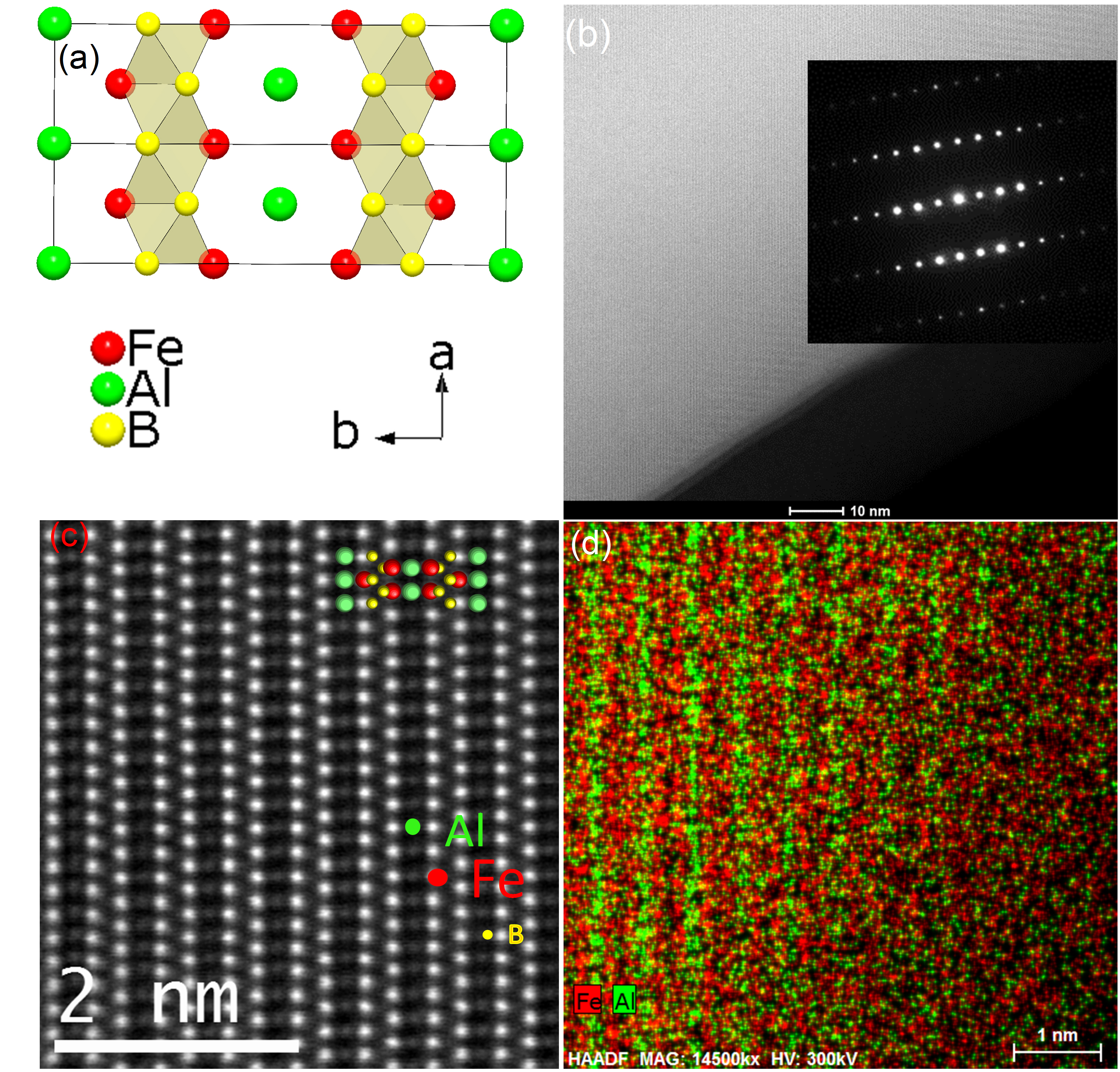
Figure 1: (a) AlFe₂B₂ unit cell (b) HAADF STEM image shows uniform chemistry of the AlFe₂B₂ crystal. The inset is a corresponding selected-area electron diffraction pattern. (c) High resolution HAADF STEM image of AlFe₂B₂ taken along [101] zone axis along with projection of a unit cell represented with Fe (red), Al(green) and B (yellow) spheres. The structural pattern of Al and FeB slab layers are also visible in unit cell shown in pannel (a). (d) EDS elemental mapping without account of B scattering effect where green stripes are Al and red stripes are Fe distributions.

II.2 Characterization and physical properties measurements

The crystal structure of AlFe₂B₂ was characterized with both single crystal X-ray diffraction (XRD) and powder XRD. The single crystal XRD data were collected within a $4^{\circ}$-$29^{\circ}$ angle value of 2$\theta$ using Bruker Smart APEX II diffractometer with graphite-monochromatized Mo-K_α radiation source ($\lambda$ = 0.71073 $\AA$). The powder diffraction data were collected using a Rigaku MiniFlex II diffractometer with Cu-K_α radiation. The acid etched AlFe₂B₂ crystals were ground to fine powder and spread over a zero background, Si-wafer sample holder with help of a thin film of Dow Corning high vacuum grease. The diffraction intensity data were collected within a 2$\theta$ interval of $5^{\circ}$-$100^{\circ}$ with a fixed dwelling time of 3 sec and a step size of $0.01^{\circ}$.

The as-grown single crystalline sample was examined with a transmission electron microscopy to obtain High-angle-annular-dark-field (HAADF) scanning transmission electron microscopy (STEM) images, corresponding selected-area electron diffraction pattern and high resolution HAADF STEM image of AlFe₂B₂ taken under [101] zone axis.

The anisotropic magnetic measurements were carried out in a Quantum Design Magnetic Property Measurement System (MPMS) for 2 K $\leq T\leq$ 300 K and a Versalab Vibrating Sample Magnetometer (VSM) for 50 K$\leq T\leq$700 K.

The temperature dependent resistivity of AlFe₂B₂ was measured in a standard four-contact configuration, with contacts prepared using silver epoxy. The excitation current was along the crystallographic a-axis. AC resistivity measurement were performed in a Quantum Design Physical Property Measurement System (PPMS) using 1 mA; 17 Hz excitation, with a cooling at a rate of 0.25 K/min. A Be-Cu/Ni-Cr-Al hybrid piston-cylinder cell similar to the one described in Ref. Bud’ko et al., 1984 was used to apply pressure. Pressure values at the transition temperature $T_{C}$ were estimated by linear interpolation between the room temperature pressure $p_{300\textrm{K}}$ and low temperature pressure $p_{T\leq 90\textrm{K}}$ valuesThompson (1984); Torikachvili et al. (2015). $p_{300\textrm{K}}$ values were inferred from the $300$ K resistivity ratio $\rho(p)/\rho(0\,\textrm{GPa})$ of leadEiling and Schilling (1981) and $p_{T\leq 90\textrm{K}}$ values were inferred from the $T_{c}(p)$ of leadBireckoven and Wittig (1988). Good hydrostatic conditions were achieved by using a 4:6 mixture of light mineral oil:n-pentane as a pressure medium; this mixture solidifies at room temperature in the range $3-4$ GPa, i.e., well above our maximum pressureBud’ko et al. (1984); Kim et al. (2011); Torikachvili et al. (2015).

III Experimental results

III.1 Structural characterization

The HAADF STEM image along with selected area diffraction pattern in the inset and high resolution HAADF STEM image of AlFe₂B₂ taken under [101] zone axis and EDS Al-Fe elmental mapping are presented in pannels (b), (c) and (d) of FIG. 1. Taken together they strongly suggest the uniform chemical composition of AlFe₂B₂ through out the sample.

The crystallographic solution and parameters refinement on the single crystalline XRD data was performed using SHELXTL program package SHE . The Rietveld refined single crystalline data are presented in TABLES 1, and 2. Using the atomic coordinates from the crystallographic information file obtained from single crystal XRD data, powder XRD data were Rietveld refined with $R_{P}$ = 0.1 using General Structure Analysis System Toby (2001) (FIG. 2 (a)). The lattice parameters from the powder XRD are: a = 2.920(4) $\AA$, b = 11.026(4) $\AA$ and c = 2.866(7) $\AA$ which are in reasonable agreement with the single crystal data analysis values.

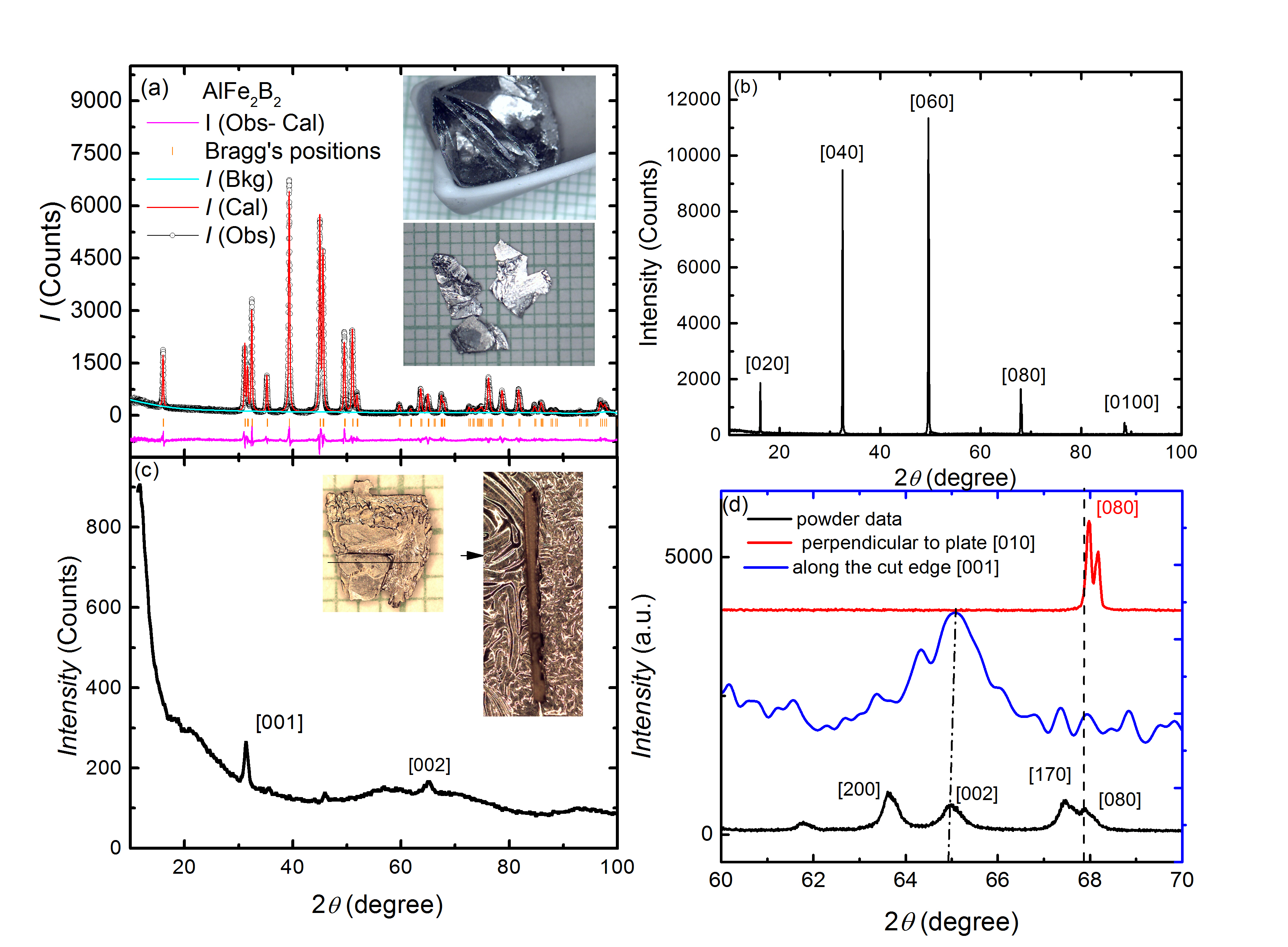
Figure 2: (a) Powder XRD for AlFe₂B₂. I(Obs), I(Cal) and I(Bkg) stands for experimental powder diffraction, Rietveld refined and instrumental background data. The green vertical lines represent the Bragg reflection peaks and the I(Obs-Cal) is the differential intensity between I(Obs) and I(Cal). The upper inset picture shows the crucible limited growth nature of AlFe₂B₂. The lower inset picture is the pieces of as grown plate-like crystals. (b) Monochromatic XRD pattern from the plate surface of AlFe₂B₂. (c) Monochromatic XRD pattern from cut surface [001] collected using Bragg-Brentano geometry. The left inset photo shows the as grown AlFe₂B₂ crystal. The right inset picture is the photograph of the cut section of the crystal parallel to (001) plane. The middle unidentified peak might be due to a differently oriented shard of cut AlFe₂B₂ crystal. (d) Comparison of the monochromatic surface XRD patterns from (b) and (c) with powder XRD pattern from (a) within extended 2$\theta$ range of 60 - 70^∘ to illustrate the identification scheme of the crystallographic orientation.

Table 1: Crystal data and structure refinement for AlFe₂B₂.

Empirical formula	AlFe2B2
Formula weight	160.3
Temperature	$293(2)$ K
Wavelength	$0.71073$ Å
Crystal system, space group	Orthorhombic, Cmmm
Unit cell dimensions	a=2.9168(6) Å
	b = 11.033(2) Å
	c = 2.8660(6) Å
Volume	92.23(3) $10^{3}$ Å3
Z, Calculated density	2, 5.75 g/$cm^{3}$
Absorption coefficient	31.321 mm-1
F(000)	300
$\theta$ range (∘)	3.693 to 29.003
Limiting indices	$-3\leq h\leq 3$
	$-14\leq k\leq 14$
	$-3\leq l\leq 3$
Reflections collected	402
Independent reflections	7 [R(int) = 0.0329]
Absorption correction	multi-scan, empirical
Refinement method	Full-matrix least-squares
	on F2
Data / restraints / parameters	74 / 0 / 12
Goodness-of-fit on $F^{2}$	1.193
Final R indices [I$>2\sigma$(I)]	$R1=0.0181$, $wR2=0.0467$
R indices (all data)	$R1=0.0180$, $wR2=0.0467$
Largest difference peak and hole	0.679 and -0.880 e.Å-3

Table 2: Atomic coordinates and equivalent isotropic displacement parameters (A²) for AlFe₂B₂. U(eq) is defined as one third of the trace of the orthogonalized U_ij tensor.

atom	Wyckoff site	x	y	z	Ueq
Fe	4(j)	0.0000	0.3539(1)	0.5000	0.006(6)
Al	2(a)	0.0000	0.0000	0.0000	0.006(7)
B	4(i)	0.0000	0.2066(5)	0.0000	0.009(7)

To confirm the crystallogrpahic orientation of the AlFe₂B₂ crystals, monochromatic Cu-$K_{\alpha}$ XRD data were collected from the flat surface of the crystals and found to be {020} family as shown in FIG. 2 (b), i.e. the [010] direction is perpendicular to the plate. However finding a thick enough, flat, as grown facet with [100] and [001] direction was made difficult by the thin, sheet-like morphology of the sample and its crucible limited growth nature. A [001] facet was cut out of large crucible limited crystal as shown in the inset of FIG. 2(c). The monochromatic Cu-$K_{\alpha}$ XRD pattern scattered from the cut surface confirms the [001] direction displaying the [001] and [002] peaks (FIG. 2 (c)). To better illustrate the crystallographic orientations, powder XRD, and monochromatic surface XRD patterns from the plate surface and cut edge are plotted together in FIG. 2 (d). This plot clearly identifies that direction perpendicular to the plate is [010] and cut edge surface is (001). Slight displacement of the surface XRD peaks is the result of the sample height in the Bragg Brentano geometry. The splitting of [080] peak is observed by distinction of Cu-$K_{\alpha}$ satellite XRD patterns usually observed at high diffraction angles.

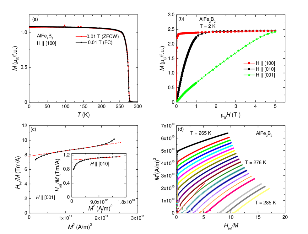
Figure 3: (a) Temperature dependent magnetization with 0.01 T applied field along [100] direction (b)) Field dependent magnetization along principle directions at $2$ K. [100] is the easy axis with smallest saturating field , [010] is the intermediate axis with 1 T anisotropy and [001] is the hardest axis with $\sim 5$ T anisotropy field. (c) Sucksmith-Thompson plot for M(H) data along [001] direction (and along [010] in the inset) to estimate the magneto-crystalline anisotropy constants. The red dash-dotted line is the linear fit to the hard axes isotherms at high field region ($>3$ T) whose Y-intercept is used to estimate the anisotropy constant $K$. (d) Arrott plot obtained with easy axis isotherms within the temperature range of 265-285 K at a step of 1 K. The straight line through the origin is the tangent to the isotherm corresponding to the transition temperature.

IV Magnetic properties

The anisotropic magnetization data were measured using a sample with known crystallographic orientation. The temperature dependent magnetization M(T) data along [100] axis is presented in FIG. 3(a). Both the Zero Field Cooled Warming (ZFCW) and Field Cooled(FC) M(T) data are almost overlapping for 0.01 T applied field. The M(T) data suggest a Curie temperature (T_C) of $\sim 275$ K using an inflection point of M(T) data as a criterion. This value will be determined more precisely below to be T_C = 274 K using easy axis M(H) isotherms around Curie temperature.

FIG. 3(b) shows the anisotropic, field-dependent magnetization at $2$ K. The saturation magnetization ($M_{sat}$) at $2$ K is determined to be $2.40$ $\mu_{B}$/f.u., i.e. roughly half of bulk BCC Fe moment. The anisotropic M(H) data at 2 K show [100] is the easy axis, [010] axis is a harder axis with an anisotropy field of $\approx 1$ T and [001] is the hardest axis of magnetization with an anisotropy field of $\approx 5$ T. A Sucksmith-Thompson plot Sucksmith and Thompson (1954), using M(H) data along [001], is shown in FIG. 3(c). The inset to FIG. 3(c) shows data for H along [010]. In a Sucksmith-Thompson plot, the Y-intercept of the linear fit of hard axis $\frac{H_{int}}{M}$ vs $M^{2}$ isotherm provides the magneto-crystalline anisotropy constant ($intercept=\frac{2K_{1}}{{M_{S}}^{2}}$, $M_{S}$ being saturation magnetization at 2 K) of the material. From these plots we determined $K_{010}$ = $0.23\leavevmode\nobreak\ MJm^{-3}$ and $K_{001}$ = $1.78\leavevmode\nobreak\ MJm^{-3}$ respectively.

Given that AlFe₂B₂ has $T_{C}\sim$ room temperature, and is formed from earth abundant elements, it is logical to examine it as a possible magnetocaloric material. The easy axis, [100], M(H) isotherms around the Curie temperature (shown for the Arrott plot in FIG. 3(d)) were used to estimate the magnetocaloric property for AlFe₂B₂ in-terms of entropy change using following equation Tan et al. (2013); Lamichhane et al. (2016a):

$$\begin{split}\Delta S(\frac{T_{1}+T_{2}}{2},\Delta H)\approx\\ &\dfrac{\mu_{0}}{T_{2}-T_{1}}\int^{H_{f}}_{H_{i}}M(T_{2},H)-M(T_{1},H)dH\\ \end{split}$$ (1)

where $H_{i}$, $H_{f}$ are initial and final applied fields and $T_{2}-T_{1}$ is the change in temperature. For this formula to be valid, $T_{2}-T_{1}$ should be small. Here $T_{2}-T_{1}$ is taken to be $1$ K. The entropy change calculation scheme in one complete cycle of magnetization and demagnetization is estimated in terms of area between two consecutive isotherms between the given field limit as shown in FIG. 4(a). The measured entropy change as a function of temperature is presented in FIG. 4(b). The entropy change in $2$ T and $3$ T applied fields is maximum around $276$ K being $3.78$ Jkg^-1K^-1 and $4.87$ Jkg^-1K^-1respectively. The 2 T applied field entropy change data of this experiment agrees very well with reference [Barua et al., 2018], shown as 2 T^∗ data in FIG. 4(b). The entropy change values for our single crystalline samples are in close agreement with previously reported polycrystalline sample measured values as well Tan et al. (2013); Du et al. (2015).

Although, AlFe₂B₂ is a rare-earth free material, its magnetocaloric property is larger than lighter rare-earth RT₂X₂ (R = rare earth T = transition metal, X = Si,Ge) compounds with ThCr₂Si₂-type structure (space group I4/mmm) namely CeMn₂Ge₂($\sim 1.8$ Jkg^-1K^-1) Md Din et al. (2015), PrMn₂Ge_0.8Si_1.2($\sim 1.0$ Jkg^-1K^-1) Wang et al. (2009) and Nd(Mn_1-xFe_x)₂Ge₂($\sim 1.0$ Jkg^-1K^-1) Chen et al. (2010). The entropy change of AlFe₂B₂ is significantly smaller than Gd₅Si₂Ge₂($\sim 13$ Jkg^-1K^-1), it has comparable entropy change with elemental Gd($\sim 5.0$ Jkg^-1K^-1) Pecharsky and Gschneidner (1997). These results shows that AlFe₂B₂ has the potential to be used for magnetocaloric material considering the abundance of its constituents.

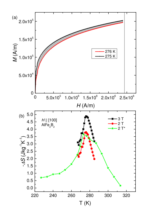
Figure 4: Magnetocaloric effect in AlFe₂B₂ obtained using M(H) isotherms along [100]. (a) showing the change in entropy ($\Delta S$) evaluation scheme at its highest value (b) change in entropy with $2$ T and $3$ T applied fields using easy axis [100] isotherms. For the sake of comparison, the 2 T^∗ field data are taken from the reference [Barua et al., 2018].

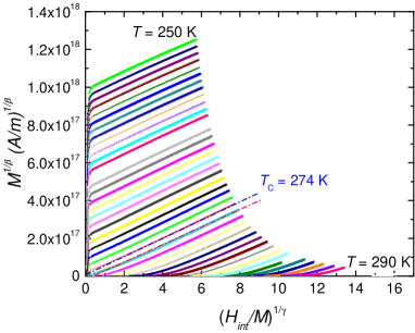
Figure 5: Generalized Arrott plot of AlFe₂B₂ with magnetization data along [100] direction within temperature range of 250 - $290$ K at a step of $1$ K. The $\beta=0.30\pm 0.04$ and $\gamma=1.180\pm 0.005$ were determined from the Kouvel-Fisher method. The two dash-dot straight lines are drawn to visualize the intersection of the isotherms with the axes.

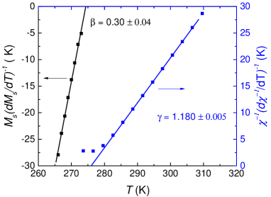
Figure 6: Determination of the critical exponents ($\beta$ and $\gamma$)using Kouvel-Fisher plots. See text for details.

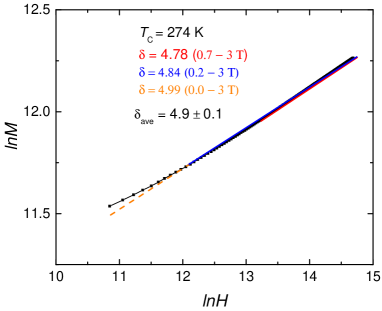
Figure 7: Determination of the critical exponent $\delta$ using Kouvel-Fisher plots using M(H) isotherm at $T_{C}$ to check the consistency of $\beta$ and $\gamma$ via Widom scaling. The data used for determining the exponent $\delta$ are highlighted with the red curve in corresponding M(H) isotherm. The data in the low field region slightly deviate from the linear behaviour in the logarithmic scale as shown in the inset. The range dependency of the value of $\delta$ is illustrated with different colors tangents. The field range for the fitted data is indicated in the parenthesis along with the value of $\delta$. See text for details.

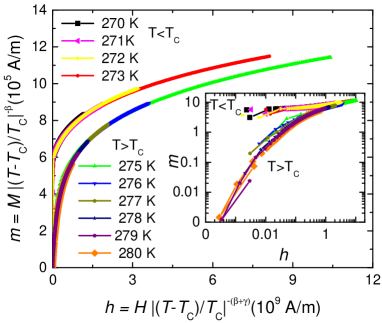
Figure 8: Normalized isotherms to check the validity of scaling hypothesis. The isotherms in between 270-$273$ K are converged to higher value (T$<$T_C) and isothems inbetween 275-$280$ K are converged to lower value(T$>$T_C). The inset shows the corresponding log-log plot clearly bifurcated in two branches in low field region.

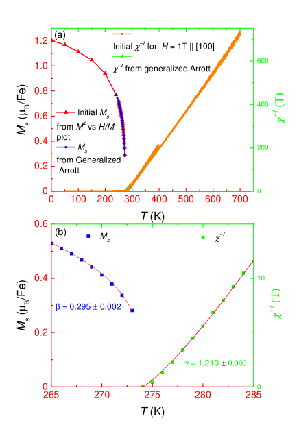
Figure 9: Illustration of the consistency of the critical exponents $\beta$ and $\gamma$ used for generalizes Arrott plot (a) by reproducing the initial spontaneous magnetization $M_{S}$ and $\chi^{-1}(T)$ via Y and X-intercept of the generalized Arrott plot. (b) Fitting of the extracted data (squares) from generalized Arrott plot with corresponding power laws (red lines) in equation 6 and 7.

To precisely determine the Curie temperature, an Arrott plot was constructed using a wider range of M(H) isotherms along the [100] direction (FIG. 3(d)). In an Arrott plot $M^{2}$ is plotted as a function of $\frac{H_{int}}{M}$. H_int= H_app-N*M is internal field inside the sample after the demagnetization field is subtracted. In this case the experimental demagnetization factor along the easy axis of the sample was found to be almost negligible because of its thin, plate-like shape with the easy axis lying along the longest dimension of the sample. The detail of determination of the experimental demagnetization factors and their comparison with theoretical data is explained in the references [Lamichhane et al., 2016a] and [Lamichhane et al., 2016b]. The Arrott plots have a positive slope indicating the transition is second order Banerjee (1964). In the mean field approximation, in the limit of low fields, the Arrott isotherm corresponding to the Curie temperature is a straight line and passes through the origin. In FIG. 3(d), the isotherm corresponding to $276$ K passes through the origin but it is not a perfectly straight line. This suggests that the magnetic interaction in AlFe₂B₂ does not obey the mean-field theory. In the mean-field theory, electron correlation and spin fluctuations are neglected, but these can be significant around the transition temperature of an itinerant ferromagnet.

Since the Arrott plot data are not straight lines, a generalized Arrott plot is an alternative way to better confirm the Curie temperature. The generalized Arrott plot derived from the equation of the state Arrott and Noakes (1967)

$$({\frac{H_{int}}{M}})^{1/\gamma}=a\frac{T-T_{C}}{T}+bM^{1/\beta}$$ (2)

is shown in FIG. 5. The critical exponents $\beta$ and $\gamma$ used in equation of state are derived from the Kouvel-Fisher analysisKouvel and Fisher (1964); Mohan et al. (1998). To determine $\beta$, the equation used was:

$$M_{S}[\frac{d}{dT}(M_{S})]^{-1}=\frac{T-T_{C}}{\beta}$$ (3)

where the slope is $\frac{1}{\beta}$. The value of the spontaneous magnetization around the transition temperature was extracted from the Y-intercept of the ${M_{S}}^{4}$ vs $\frac{H}{M}$ Chen et al. (2013) exploiting their straight line nature with clear Y-intercept. The experimental value of $\beta$ was determined to be $0.30\pm 0.04$ as shown in FIG. 6. The uncertainty in $\beta$ was determined with fitting error as $\Delta\beta$ = $\frac{\delta slope}{{slope}^{2}}$.

Similarly, the value of critical exponent $\gamma$ was determined with the equation:

$${\chi}^{-1}[\frac{d}{dT}({\chi}^{-1})]^{-1}=\frac{T-T_{C}}{\gamma}$$ (4)

where the slope is $\frac{1}{\gamma}$ and $\chi^{-1}(T)$ is the initial high temperature inverse susceptibility near the transition temperature. The experimental value of the $\gamma$ was determined to be $1.180\pm 0.005$ as shown in FIG. 6.

Finally the third critical exponent $\delta$ was determined using the equation:

$$M\propto H^{1/\delta}$$ (5)

by plotting ln(M) vs ln(H) (FIG. 7) corresponding to Curie temperature $274$ K. The experimental value of the $\delta$ was determined by fitting ln(M) vs ln(H) over different ranges of applied field H. Taking the average of the range of the $\delta$ value as shown in FIG. 7 we determine $\delta$ to be $4.9\pm 0.1$ which was closely reproduced ($4.93\pm 0.03$) with Widom scaling theory $\delta=1+\frac{\gamma}{\beta}$.

Additionally, the validity of Widom scaling theory demands that the magnetization data should follow the scaling equation of the state. The scaling laws for a second order magnetic phase transition relate the spontaneous magnetization M_S(T) below T_C, the inverse initial susceptibility ${\chi}^{-1}(T)$ above T_C, and the magnetization at T_C with corresponding critical amplitudes by the following power laws:

$$M_{S}(T)=M_{0}(-\epsilon)^{\beta},\epsilon<0$$ (6)

$${\chi}^{-1}(T)=\Gamma(\epsilon)^{\gamma},\epsilon>0$$ (7)

$$M=XH^{\frac{1}{\delta}}$$ (8)

Where M₀, $\Gamma$ and X are the critical amplitudes and $\epsilon=\frac{T-T_{C}}{T_{C}}$ is the reduced temperature Pramanik and Banerjee (2009). The scaling hypothesis assumes the homogeneous order parameter which with scaling hypothesis can be expressed as

$$M(H,\epsilon)={\epsilon}^{\beta}f_{\pm}(\frac{H}{{\epsilon}^{\beta+\gamma}})$$ (9)

Where $f_{+}$(T$>T_{C}$) and $f_{-}$(T$<T_{C}$) are the regular functions. With new renormalised parameters, m = ${\epsilon}^{-\beta}M(H,\epsilon)$ and h = ${\epsilon}^{-(\beta+\gamma)}M(H,\epsilon)$ equation 9 can be written as

$$m=f_{\pm}(h)$$ (10)

Up to the linear order, the scaled m vs h graph is plotted as shown in FIG 8 along with an inset in log-log scale which clearly shows that all isotherms converge to the two curves one for T$>T_{C}$ and other for T$<T_{C}$. This graphically shows that all the critical exponents were properly renormalized.

Finally the consistency of the critical exponents $\beta$ and $\gamma$ is demonstrated (shown in FIG. 9(a)) by reproducing the initial spontaneous magnetization $M_{S}$ and $\chi^{-1}(T)$ near the transition temperature using the Y and X-intercept of generalized Arott plots as shown in FIG. 5 which overlaps with $M_{S}$ obtained by ${M_{S}}^{4}$ vs $\frac{H}{M}$ [Chen et al., 2013] and and initial inverse susceptibility $\chi^{-1}(T)$ with 1 T applied field. The extracted data well fit Pramanik and Banerjee (2009) with corresponding power laws in equation (6) and (7) as shown in FIG. 9(b) giving $\beta=0.295\pm 0.002$ and $\gamma=1.210\pm 0.003$ which closely agree with previously obtained K-F values.

To measure the effective moment ($M_{eff}$) of the Fe above the Curie temperature, a Curie-Weiss plot was prepared as shown in FIG. 9. The effective moment of the Fe-ion above the Curie temperature was determined to be $2.15$ $\mu_{B}$. Since the effective moment above the Curie temperature is almost equal to BCC Fe ($2.2$ $\mu_{B}$) and the ordered moment at $2$ K is significantly smaller than Fe-ion ($1.2$ $\mu_{B}$/Fe) giving the Rhode-Wohlfarth ratio ($\frac{M_{C}}{M_{sat}}$) nearly equal to 1.14, where $M_{C}(M_{C}+2)={M_{eff}}^{2}$, this compound shows signs of an itinerant nature in its magnetization Rhodes and Wohlfarth (1963).

Itinerant magnetism, in general, can be tuned (meaning the size of magnetic moment and Curie temperature can be altered significantly and sometime even suppressed completely) with an external parameter like pressure or chemical doping. As a case study, we investigated the influence of the external pressure on the ferromagnetism of AlFe₂B₂.

Figure 10 shows the pressure dependent resistivity of single crystalline AlFe₂B₂ with current applied along the crystallographic $a$-axis. It shows metallic behaviour with a residual resistivity of 60 $\mu\Omega$ cm. The ambient pressure temperature dependent resistivity of AlFe₂B₂ shows a kink around $275$ K, indicating a loss of spin disorder scattering associated with the onset of ferromagnetic order. As pressure is increased to 2.24 GPa the temperature of this kink is steadily reduced. To determine the transition temperature $T_{C}$, the maximum in the temperature derivative $d\rho$/$dT$ is used, as shown in the inset of FIG. 10. The pressure dependence of $T_{C}$, the temperature - pressure phase diagram of AlFe₂B₂ is presented in FIG. 11. The transition temperature, $T_{C}$, is suppressed from $275$ K to $255$ K when pressure is increased from 0 to $2.24$ GPa, giving a suppression rate of -8.9 K/GPa. Interestingly, Curie temperature suppression rate of AlFe₂B₂ is found to be comparable to the model itinerant magnetic materials like helimagnetic MnSi ($\sim-15$ K/GPa) Pfleiderer et al. (2004), and weak ferromagnets ZrZn₂ ($\sim-13$ K/GPa) Uhlarz et al. (2004) and Ni₃Al ($\sim-4$ K/GPa) Niklowitz et al. (2005). A linear fitting of the data as shown in FIG. 11 indicates that to completely suppress the $T_{C}$ around 31 GPa would be required. Usually such linear extrapolation provide an upper estimate of the critical pressure.

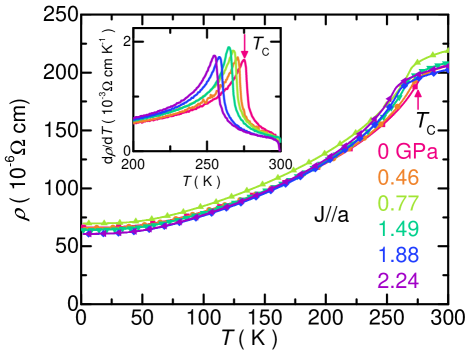
Figure 10: Evolution of the single crystal AlFe₂B₂ resistivity with hydrostatic pressure up to $2.24$ GPa. Pressure values at $T_{C}$ were estimated from linear interpolation between the $P_{300\textrm{K}}$ and $P_{T\leq 90\textrm{K}}$ values (see text). Current was applied along the crystallographic $a$-axis. Inset shows the evolution of temperature derivative $d\rho$/$dT$ with hydrostatic pressure. The peak positions in the derivative were identified as transition temperature $T_{C}$. Examples of $T_{C}$ are indicated by arrows in the figure.

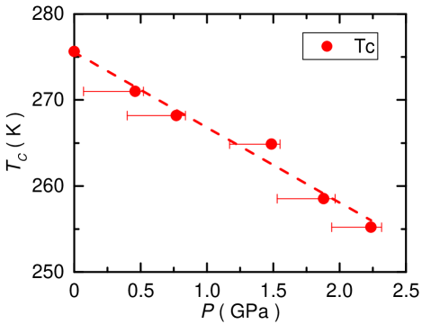
Figure 11: Temperature - pressure phase diagram of AlFe₂B₂ as determined from resistivity measurement. Pressure values were estimated as being described in Fig. 10 and in the text. Error bars indicate the room temperature pressure $P_{300\textrm{K}}$ and low temperature pressure $P_{T\leq 90\textrm{K}}$. As shown in the figure, in the pressure region of $0-2.24$ GPa the ferromagnetic transition temperature $T_{C}$ is suppressed upon increasing pressure, with suppressing rate around $-8.9$ K/GPa.

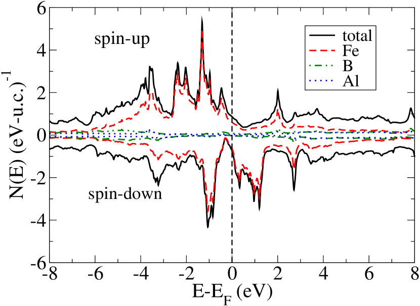
Figure 12: The calculated density-of-states of AlFe₂B₂.

First principles calculations

Theoretical calculations for AlFe₂B₂ were performed using the all electron density functional theory code WIEN2K Blaha et al. (2001); Sjostedt et al. (2000); Singh and Nordstrom (2006). The generalized gradient approximation according to Perdew, Burke, and Ernzerhof (PBE) Perdew et al. (1996) was used in our calculations. The sphere radii (RMT) were set to 2.21, 2.17, and 1.53 Bohr for Fe, Al, and B, respectively. RK_max which defines the product of the smallest sphere radius and the largest plane wave vector was set to 7.0. All calculations were performed with the experimental lattice parameters as reported in reference [Cedervall et al., 2016b] (which are consistent with our results) and all internal coordinates were relaxed until internal forces on atoms were less than 1 mRyd/Bohr-radius. All the calculations were performed in the collinear spin alignment. The magnetic anisotropy energy (MAE) was obtained by calculating the total energies of the system with spin-orbit coupling (SOC) with the magnetic moment along the three principal crystallographic axes. For these MAE calculations the $k$-point convergence was carefully checked, and the calculations reported here were performed with 120,000 $k$-points in the full Brillouin zone.

Similar to the experimental observation, AlFe₂B₂ is calculated to have ferromagnetic behaviour, with a saturation magnetic moment (we do not include the small Fe orbital moment) of 1.36 $\mu_{B}$/Fe. This is in reasonable agreement with the experimentally measured value of 1.21$\mu$B/Fe. Interestingly this calculated magnetic moment on Fe, is significantly lower than the moment on Fe in BCC Fe (2.2 $\mu_{B}$/Fe ) further suggesting a degree of itinerant behaviour. The calculated density of states is shown in FIG. 12. As expected for a Fe-based ferromagnet, the electronic structure in the vicinity of the Fermi level is dominated by Fe $d$ orbitals and we observe a substantial exchange splitting of 2-3 eV.

For an orthorhombic crystal structure, the magnetic anisotropy energy is described by total energy calculations for the magnetic moments along each of the three principal axis Palmer (1963). For AlFe₂B₂ we find, the [100] and [010] axes to be the “easy” directions, separated by just 0.016 meV per Fe, with [100] being the easiest axis. The [001] direction is the “hard” direction, which lies 0.213 meV per Fe above the [100] axis. As in our previous work on HfMnP Lamichhane et al. (2016a), this value is much larger than the 0.06 meV value for hcp Co and likely results from a combination of the orthorhombic crystal structure and the structural complexity associated with a ternary compound. The 0.213 meV energy difference on a volumetric basis corresponds to a anisotropy constant K₁ as 1.48 MJ/m³. (Note that we use the convention of the previous work and simply define K₁ for an orthorhombic system as the energy difference between the hardest and easiest directions.) This magnetic anisotropy constant describes the energy cost associated with the changing the orientation of the magnetic moments under the application of a magnetic field, and is an essential component for permanent magnets. It is noteworthy that this anisotropy is comparable to the value of 2 MJ/m³ proposed by Coey for an efficient permanent magnet Coey (2011), despite containing no heavy elements, using the approximation that $H_{a}\approx 2\mu_{0}K_{1}/M_{s}$, with K as 1.48 MJ/m³ and M_s as 0.68 T, yields an anisotropy field of 5.4 T, which is in excellent agreement with the experimentally measured value of 5 T and $K_{001}\approx 1.8\leavevmode\nobreak\ MJ/m^{3}$.

V Conclusions

Single crystalline AlFe₂B₂ was grown by self-flux-growth technique and structural, magnetic and transport properties were studied. AlFe₂B₂ is an orthorhombic, metallic ferromagnet with promising magnetocaloric behaviour. The Curie temperature of AlFe₂B₂ was determined to be $274$ K using the generalized Arrott plot method along with estimation of critical exponents using Kouvel-Fisher analysis. The ordered magnetic moment ($M_{sat}$) at $2$ K is $1.20\mu_{B}$/Fe at $2$ K which is much less than paramagnetic Fe-ion moment at high temperature ($2.15\mu_{B}$/Fe) indicating itinerant magnetism. The magnetization in AlFe₂B₂ responds to the hydrostatic pressure with $\frac{dT_{C}}{dP}\sim-8.9$ K/GPa. A linear extrapolation of this $T_{C}(P)$ trend leads to an upper estimate of $\sim 30$ GPa required to fully supress the transition. The saturation magnetization and anisotropic magnetic field predicted by first principle calculations are in close agreement with the experimental results. The magneto-crystalline anisotropy fields were determined to be $1$ T along [010] and $5$ T along [001] direction w. r. to easy axis [100]. The magneto-crystalline anisotropy constants at 2 K are determined to be $K_{010}\approx 0.23\leavevmode\nobreak\ MJ/m^{3}$ and $K_{001}\approx 1.8\leavevmode\nobreak\ MJ/m^{3}$.

VI Acknowledgement

We would like to thank Drs. W. R. McCallum and L. H. Lewis for drawing attention to this compound and Dr. A. Palasyuk for useful discussions. This research was supported by the Critical Materials Institute, an Energy Innovation Hub funded by the U.S. Department of Energy, Office of Energy Efficiency and Renewable Energy, Advanced Manufacturing Office. This work was also supported by the office of Basic Energy Sciences, Materials Sciences Division, U.S. DOE. Li Xiang was supported by W. M. Keck Foundation. This work was performed at the Ames Laboratory, operated for DOE by Iowa State University under Contract No. DE-AC02-07CH11358.

References

- Tan et al. (2013) Xiaoyan Tan, Ping Chai, Corey M. Thompson, and Shatruk Michael, “Magnetocaloric Effect in AlFe2B2: Toward Magnetic Refrigerants from Earth-Abundant Elements,” J. Am. Chem. Soc. 135, 9553–9557 (2013), http://dx.doi.org/10.1021/ja404107p .
- Cedervall et al. (2016a) Johan Cedervall, Lennart Häggström, Tore Ericsson, and Martin Sahlberg, “Mössbauer study of the magnetocaloric compound AlFe2B2,” Hyperfine Interactions 237, 47 (2016a).
- ElMassalami et al. (2011) M. ElMassalami, D. da S. Oliveira, and H. Takeya, “On the ferromagnetism of AlFe2B2 ,” J. Magn. Magn. Mater. 323, 2133 – 2136 (2011).
- Jeitschko (1969) Wolfgang Jeitschko, “The crystal structure of Fe2AlB2.” Acta Cryst. B, 163–165 (1969).
- Kuz’ma and Chaban (1969) Yu. B. Kuz’ma and N.F. Chaban, “Crystal Structure of the Compound Fe2AlB2,” Inorg. Mater. 5, 321–322 (1969).
- Du et al. (2015) Qianheng Du, Guofu Chen, Wenyun Yang, Jianzhong Wei, Muxin Hua, Honglin Du, Changsheng Wang, Shunquan Liu, Jingzhi Han, Yan Zhang, and Jinbo Yang, “Magnetic frustration and magnetocaloric effect in AlFe2-x Mnx B2 ( x = 0 - 0.5) ribbons,” Journal of Physics D: Applied Physics 48, 335001 (2015).
- Hirt et al. (2016) Sarah Hirt, Fang Yuan, Yurij Mozharivskyj, and Harald Hillebrecht, “AlFe2-xCoxB2 (x = 0 - 0.30): TC Tuning through Co Substitution for a Promising Magnetocaloric Material Realized by Spark Plasma Sintering,” Inorg. Chem. 55, 9677–9684 (2016), pMID: 27622951, http://dx.doi.org/10.1021/acs.inorgchem.6b01467 .
- Barua et al. (2018) R. Barua, B.T. Lejeune, L. Ke, G. Hadjipanayis, E.M. Levin, R.W. McCallum, M.J. Kramer, and L.H. Lewis, “Anisotropic magnetocaloric response in AlFe2B2,” J. Alloys Compd. 745, 505 – 512 (2018).
- Levin et al. (2018) E. M. Levin, B. A. Jensen, R. Barua, B. Lejeune, A. Howard, R. W. McCallum, M. J. Kramer, and L. H. Lewis, “Effects of Al content and annealing on the phases formation, lattice parameters, and magnetization of A lxFe2 B2( x = 1.0 , 1.1 , 1.2 ) alloys,” Phys. Rev. Materials 2, 034403 (2018).
- Canfield and Fisk (1992) P. C. Canfield and Z. Fisk, “Growth of single crystals from metallic fluxes,” Philos. Mag. 65, 1117–1123 (1992), http://dx.doi.org/10.1080/13642819208215073 .
- Canfield et al. (2016) Paul C. Canfield, Tai Kong, Udhara S. Kaluarachchi, and Na Hyun Jo, “Use of frit-disc crucibles for routine and exploratory solution growth of single crystalline samples,” Philos. Mag. 96, 84–92 (2016).
- Bud’ko et al. (1984) S.L. Bud’ko, A.N. Voronovskii, A.G. Gapotchenko, and E.S. ltskevich, “The fermi surface of cadmium at an electron-topological phase transition under pressure,” J. Exp. Theor. Phys. 59, 454 (1984).
- Thompson (1984) J. D. Thompson, “Low-temperature pressure variations in a self-clamping pressure cell,” Rev. Sci. Instrum. 55, 231–234 (1984), https://doi.org/10.1063/1.1137730 .
- Torikachvili et al. (2015) M. S. Torikachvili, S. K. Kim, E. Colombier, S. L. Bud’ko, and P. C. Canfield, “Solidification and loss of hydrostaticity in liquid media used for pressure measurements,” Rev. Sci. Instrum. 86, 123904 (2015), http://dx.doi.org/10.1063/1.4937478 .
- Eiling and Schilling (1981) A Eiling and J S Schilling, “Pressure and temperature dependence of electrical resistivity of Pb and Sn from 1-300K and 0-10 GPa-use as continuous resistive pressure monitor accurate over wide temperature range; superconductivity under pressure in Pb, Sn and In,” J. Phys. F: Met. Phys 11, 623 (1981).
- Bireckoven and Wittig (1988) B Bireckoven and J Wittig, “A diamond anvil cell for the investigation of superconductivity under pressures of up to 50 GPa: Pb as a low temperature manometer,” J Phys E 21, 841 (1988).
- Kim et al. (2011) S. K. Kim, M. S. Torikachvili, E. Colombier, A. Thaler, S. L. Bud’ko, and P. C. Canfield, “Combined effects of pressure and Ru substitution on BaFe2As2,” Phys. Rev. B 84, 134525 (2011).
- (18) SHELXTL-v2008/4, Bruker AXS Inc., Madison, Wisconsin, USA, 2013.
- Toby (2001) Brian H. Toby, “EXPGUI, a graphical user interface for GSAS,” J. Appl. Crystallogr. 34, 210–213 (2001).
- Sucksmith and Thompson (1954) W. Sucksmith and J. E. Thompson, “The Magnetic Anisotropy of Cobalt,” Proc. Royal Soc. A 225, 362–375 (1954).
- Lamichhane et al. (2016a) Tej N. Lamichhane, Valentin Taufour, Morgan W. Masters, David S. Parker, Udhara S. Kaluarachchi, Srinivasa Thimmaiah, Sergey L. Bud’ko, and Paul C. Canfield, “Discovery of ferromagnetism with large magnetic anisotropy in zrmnp and hfmnp,” Appl. Phys. Lett. 109, 092402 (2016a), http://dx.doi.org/10.1063/1.4961933 .
- Md Din et al. (2015) M. F. Md Din, J. L. Wang, Z. X. Cheng, S. X. Dou, S. J. Kennedy, M. Avdeev, and S. J. Campbell, “Tuneable Magnetic Phase Transitions in Layered CeMn2Ge2-xSix Compounds,” Sci. Rep 5 (2015), 10.1038/srep11288.
- Wang et al. (2009) J. L. Wang, S. J. Campbell, R. Zeng, C. K. Poh, S. X. Dou, and S. J. Kennedy, “Re-entrant ferromagnet PrMn2Ge0.8Si1.2: Magnetocaloric effect,” J. Appl. Phys. 105, 07A909 (2009), https://doi.org/10.1063/1.3059610 .
- Chen et al. (2010) Y.Q. Chen, J. Luo, J.K. Liang, J.B. Li, and G.H. Rao, “Magnetic properties and magnetocaloric effect of Nd(Mn1-xFex)2Ge2 compounds,” J. Alloys Compd. 489, 13 – 19 (2010).
- Pecharsky and Gschneidner (1997) V. K. Pecharsky and K. A. Gschneidner, Jr., “Giant Magnetocaloric Effect in ,” Phys. Rev. Lett. 78, 4494–4497 (1997).
- Lamichhane et al. (2016b) Tej N. Lamichhane, Valentin Taufour, Srinivasa Thimmaiah, David S. Parker, Sergey L. Bud’ko, and Paul C. Canfield, “A study of the physical properties of single crystalline Fe5B2P,” J. Magn. Magn. Mater. 401, 525 – 531 (2016b).
- Banerjee (1964) B.K. Banerjee, “On a generalised approach to first and second order magnetic transitions,” Phys. Lett. 12, 16 – 17 (1964).
- Arrott and Noakes (1967) Anthony Arrott and John E. Noakes, “Approximate equation of state for nickel near its critical temperature,” Phys. Rev. Lett. 19, 786–789 (1967).
- Kouvel and Fisher (1964) James S. Kouvel and Michael E. Fisher, “Detailed magnetic behavior of nickel near its curie point,” Phys. Rev. 136, A1626–A1632 (1964).
- Mohan et al. (1998) Ch.V Mohan, M Seeger, H Kronmüller, P Murugaraj, and J Maier, “Critical behaviour near the ferromagnetic–paramagnetic phase transition in La0.8Sr0.2MnO3 ,” J. Magn. Magn. Mater 183, 348 – 355 (1998).
- Chen et al. (2013) Bin Chen, JinHu Yang, HangDong Wang, Masaki Imai, Hiroto Ohta, Chishiro Michioka, Kazuyoshi Yoshimura, and MingHu Fang, “Magnetic Properties of Layered Itinerant Electron Ferromagnet Fe3GeTe2,” J. Phys. Soc. Jpn. 82, 124711 (2013), http://dx.doi.org/10.7566/JPSJ.82.124711 .
- Pramanik and Banerjee (2009) A. K. Pramanik and A. Banerjee, “Critical behavior at paramagnetic to ferromagnetic phase transition in : A bulk magnetization study,” Phys. Rev. B 79, 214426 (2009).
- Rhodes and Wohlfarth (1963) P. Rhodes and E. P. Wohlfarth, “The effective curie-weiss constant of ferromagnetic metals and alloys,” Proc. Roy. Soc. A. Mathematical, Physical and Engineering Sciences (1963), 10.1098/rspa.1963.0086.
- Pfleiderer et al. (2004) C. Pfleiderer, D. Reznik, L. Pintschovius, H. v. Löhneysen, M. Garst, and A. Rosch, “Partial order in the non-Fermi-liquid phase of MnSi,” Nature 427, 227–231 (2004).
- Uhlarz et al. (2004) M. Uhlarz, C. Pfleiderer, and S. M. Hayden, “Quantum Phase Transitions in the Itinerant Ferromagnet ,” Phys. Rev. Lett. 93, 256404 (2004).
- Niklowitz et al. (2005) P. G. Niklowitz, F. Beckers, G. G. Lonzarich, G. Knebel, B. Salce, J. Thomasson, N. Bernhoeft, D. Braithwaite, and J. Flouquet, “Spin-fluctuation-dominated electrical transport of at high pressure,” Phys. Rev. B 72, 024424 (2005).
- Blaha et al. (2001) P. Blaha, K. Schwarz, G. K. H. Madsen, D. Kvasnicka, and J. Luitz, WIEN2K, An Augmented Plane Wave + Local Orbitals Program for Calculating Crystal Properties (Karlheinz Schwarz, Techn. Universität Wien, Austria, 2001).
- Sjostedt et al. (2000) E Sjostedt, L Nordstrom, and David. J Singh, “An alternative way of linearizing the augmented plane-wave method,” Solid State Commun. 114, 15 – 20 (2000).
- Singh and Nordstrom (2006) David J. Singh and L. Nordstrom, Planewaves Pseudopotentials and the LAPW Method, 2nd ed. (Springer, Berlin, 2006).
- Perdew et al. (1996) John P Perdew, Kieron Burke, and Matthias Ernzerhof, “Generalized gradient approximation made simple,” Phys. Rev. Lett. 77, 3865 (1996).
- Cedervall et al. (2016b) Johan Cedervall, Mikael Svante Andersson, Tapati Sarkar, Erna K Delczeg-Czirjak, Lars Bergqvist, Thomas C Hansen, Premysl Beran, Per Nordblad, and Martin Sahlberg, “Magnetic structure of the magnetocaloric compound AlFe2B2,” J. Alloys Compd. 664, 784–791 (2016b).
- Palmer (1963) Wilfred Palmer, “Magnetocrystalline anisotropy of magnetite at low temperature,” Phys. Rev. 131, 1057 (1963).
- Coey (2011) J. M. D. Coey, “Hard magnetic materials: A perspective,” IEEE Trans. Magn. 47, 4671–4681 (2011).