Robust 6D Object Pose Estimation
with Stochastic Congruent Sets

Abstract

Object pose estimation is frequently achieved by first segmenting an RGB image and then, given depth data, registering the corresponding point cloud segment against the object’s 3D model. Despite the progress due to CNNs, semantic segmentation output can be noisy, especially when the CNN is only trained on synthetic data. This causes registration methods to fail in estimating a good object pose. This work proposes a novel stochastic optimization process that treats the segmentation output of CNNs as a confidence probability. The algorithm, called Stochastic Congruent Sets (StoCS), samples pointsets on the point cloud according to the soft segmentation distribution and so as to agree with the object’s known geometry. The pointsets are then matched to congruent sets on the 3D object model to generate pose estimates. StoCS is shown to be robust on an APC dataset, despite the fact the CNN is trained only on synthetic data. In the YCB dataset, StoCS outperforms a recent network for 6D pose estimation and alternative pointset matching techniques.

1 Introduction

Accurate object pose estimation is critical in the context of many tasks, such as augmented reality or robotic manipulation. As demonstrated during the the Amazon Picking Challenge (APC) [Correll et al.(2016)Correll, Bekris, Berenson, Brock, Causo, Hauser, Osada, Rodriguez, Romano, and Wurman], current solutions to 6D pose estimation face issues when exposed to a clutter of similar-looking objects in complex arrangements within tight spaces.

Solving such problems frequently involves two sub-components, image-based object recognition and searching in SE(3) to estimate a unique pose for the target object. Many recent approaches [Zeng et al.(2017)Zeng, Yu, Song, Suo, Walker Jr, Rodriguez, and Xiao, Hernandez et al.(2016)Hernandez, Bharatheesha, Ko, Gaiser, Tan, van Deurzen, de Vries, Van Mil, van Egmond, Burger, et al., Long et al.(2015)Long, Shelhamer, and Darrell, Ren et al.(2015)Ren, He, Girshick, and Sun] treat object segmentation by using a Convolutional Neural Network (CNN), which provides a per-pixel classification. Such a hard segmentation approach can lead to under-segmentation or over-segmentation, as shown in Fig. 1.

Segmentation is followed by a 3D model alignment using point cloud registration, such as ICP [Besl and McKay(1992)], or global search alternatives, such as 4-points congruent sets (4-PCS) [Aiger et al.(2008)Aiger, Mitra, and Cohen-Or, Mellado et al.(2014)Mellado, Aiger, and Mitra]. These methods operate over two deterministic point sets $S$ and $M$. They sample iteratively, a base $B$ of 4 coplanar points on $S$ and try to find a set of 4 congruent points on $M$, given geometric constraints, so as to identify a relative transform between $S$ and $M$ that gives the best alignment score. The pose estimate from such a process is incorrect when the segment is noisy or if it does not contain enough points from the object.

The key observation of this work is that CNN output can be seen as a probability for an object to be visible at each pixel. These segmentation probabilities can then be used during the registration process to achieve robust and fast pose estimation. This requires sampling a base $B$ on a segment, such that all points on the base belong to the target object with high probability. The resulting approach, denoted as “Stochastic Congruent Sets” (StoCS), achieves this by building a probabilistic graphical model given the obtained soft segmentation and information from the pre-processed geometric object models. The pre-processing corresponds to building a global model descriptor that expresses oriented point pair features [Drost et al.(2010)Drost, Ulrich, Navab, and Ilic]. This geometric modeling, not only biases the base samples to lie within the object bound, but is also used to constrain the search for finding the congruent sets, which provides a substantial computational benefit.

Thus, this work presents two key insights: 1) it is not necessary to make hard segmentation decisions prior to registration, instead the pose estimation can operate over the continuous segmentation confidence output of CNNs. 2) Combining a global geometric descriptor with the soft segmentation output of CNNs intrinsically improves object segmentation during registration without a computational overhead.

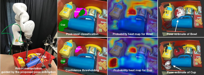
Figure 1: (a) A robotic arm using pose estimates from StoCS to perform manipulation. (b) Hard segmentation errors adversely affect model registration. (c) Heatmaps showing the continuous probability distribution for an object. (d) Pose estimates obtained by StoCS.

StoCS is first tested on a dataset of cluttered real-world scenes by using the output of an FCN that was trained solely on a synthetic dataset. In such cases, the resulting segmentation is quite noisy. Nevertheless, experiments show that high accuracy in pose estimation can be achieved with StoCS. The method has also been evaluated on the YCB object dataset [Xiang et al.(2018)Xiang, Schmidt, Narayanan, and Fox], a benchmark for robotic manipulation, where it outperforms modern pointset registration and pose estimation techniques in accuracy. It is much faster than competing registration processes, and only slightly slower than end-to-end learning.

2 Related Work

A pose estimation approach is to match feature points between textured 3D models and images [Lowe(1999), Rothganger et al.(2006)Rothganger, Lazebnik, Schmid, and Ponce, Collet et al.(2011)Collet, Martinez, and Srinivasa]. This requires textured objects and good lighting, which motivates the use of range data. Some range-based techniques compute correspondences between local point descriptors on the scene and the object model. Given correspondences, robust detectors [Ballard(1981), Fischler and Bolles(1981)] are used to compute the rigid transform consistent with the most correspondences. Local descriptors [Tombari et al.(2010)Tombari, Salti, and Di Stefano, Rusu et al.(2009)Rusu, Blodow, and Beetz, Johnson and Hebert(1999)] can be used but they depend on local surface information, which is heavily influenced by resolution and quality of sensor and model data [Aldoma et al.(2012)Aldoma, Marton, Tombari, Wohlkinger, Potthast, Zeisl, Rusu, Gedikli, and Vincze]. The features are often parametrized by the area of influence, which is not trivial to decide.

A way to counter these limitations is to use oriented point-pair features [Drost et al.(2010)Drost, Ulrich, Navab, and Ilic] to create a map that stores the model points that exhibit each feature. This map can be used to match the scene features and uses a fast voting scheme to get the object pose. This idea was extended to incorporate color [Choi and Christensen(2012)], geometric edge information [Drost and Ilic(2012)] and visibility context [Birdal and Ilic(2015), Kim and Medioni(2011)]. Recent work [Hinterstoisser et al.(2016)Hinterstoisser, Lepetit, Rajkumar, and Konolige] samples scene points by reasoning about the model size. Point-pair features have been criticized for performance loss in the presence of clutter, sensor noise and due to their quadratic complexity.

Template matching, such as LINEMOD [Hinterstoisser et al.(2012b)Hinterstoisser, Lepetit, Ilic, Holzer, Bradski, Konolige, and Navab, Hinterstoisser et al.(2012a)Hinterstoisser, Cagniart, Ilic, Sturm, Navab, Fua, and Lepetit], samples viewpoints around a 3D CAD model and builds templates for each viewpoint based on color gradient and surface normals. These are later matched to compute object pose. This approach tends not to be robust to occlusions and change in lighting.

There are also end-to-end pose estimation pipelines [Xiang et al.(2018)Xiang, Schmidt, Narayanan, and Fox, Kehl et al.(2017)Kehl, Manhardt, Tombari, Ilic, and Navab] and some approaches based on learning for predicting 3D object coordinates in the local model frame [Brachmann et al.(2014)Brachmann, Krull, Michel, Gumhold, Shotton, and Rother, Tejani et al.(2014)Tejani, Tang, Kouskouridas, and Kim, Krull et al.(2015)Krull, Brachmann, Michel, Ying Yang, Gumhold, and Rother]. A recent variant [Michel et al.(2017)Michel, Kirillov, Brachmann, Krull, Gumhold, Savchynskyy, and Rother] performs geometric validation on these predictions by solving a conditional random field. Training for such tasks requires labeling of 6D object poses in captured images, which are representative of the real-world clutter. Such datasets are difficult to acquire and involve a large amount of manual effort. There are efforts in integrating deep learning with global search for the discovery of poses of multiple objects [Narayanan and Likhachev(2016)] but they tend to be time consuming and only deal with 3D poses.

Many recent pose estimation techniques [Zeng et al.(2017)Zeng, Yu, Song, Suo, Walker Jr, Rodriguez, and Xiao, Hernandez et al.(2016)Hernandez, Bharatheesha, Ko, Gaiser, Tan, van Deurzen, de Vries, Van Mil, van Egmond, Burger, et al., Mitash et al.(2018)Mitash, Boularias, and Bekris] integrate CNNs for segmentation with pointset registration such as Iterative Closest Points (ICP) [Besl and McKay(1992)] and its variants [Rusinkiewicz and Levoy(2001), Mitra et al.(2004)Mitra, Gelfand, Pottmann, and Guibas, Segal et al.(2009)Segal, Haehnel, and Thrun, Bouazix et al.(2013)Bouazix, Tagliasacchi, and Pauly, Srivatsan et al.(2017)Srivatsan, Vagdargi, and Choset], which typically require a good initialization. Otherwise, registration requires finding the best aligning rigid transform over the 6-DOF space of all possible transforms, which are uniquely determined by 3 pairs of (non-degenerate) corresponding points. A popular strategy is to invoke RANSAC to find aligning triplets of point pairs [Irani and Raghavan(1996)] but suffers from a frequently observable worst case $O(n^{3})$ complexity in the number $n$ of data samples, which has motivated many extensions [Gelfand et al.(2005)Gelfand, Mitra, Guibas, and Pottmann, Cheng et al.(2013)Cheng, Chen, Martin, Lai, and Wang].

The 4PCS algorithm [Aiger et al.(2008)Aiger, Mitra, and Cohen-Or] achieved $O(n^{2})$ output-sensitive complexity using 4 congruent points basis instead of 3. This method was extended to Super4PCS [Mellado et al.(2014)Mellado, Aiger, and Mitra], which achieves $O(n)$ output-sensitive complexity. Congruency is defined as the invariance of the ratios of the line segments resulting from the intersections of the edges connecting the 4 points. There are 2 critical limitations: (a) The only way to ensure the base contains points from the object is by repeating the complete registration process with several initial hypotheses; (b) The number of congruent 4-points in the model can be very large for certain bases and object geometries, which increases computation time.

The current work fuses the idea of global geometric modeling of objects along with a sampling-based registration technique to build a robust pose estimator. This fusion can still enjoy the success of deep learning but also remain immune to its limitations.

3 Approach

Consider the problem of estimating the 6D poses of $N$ known objects $\{O_{1},\ldots,O_{N}\}$, captured by an RGB-D camera in an image $I$, given their 3D models $\{M_{1},\ldots,M_{N}\}$. The estimated poses are returned as a set of rigid-body transformations $\{T_{1},\ldots,T_{N}\}$, where each $T_{i}=(t_{i},R_{i})$ captures the translation $t_{i}\in R^{3}$ and rotation $R_{i}\in SO(3)$ of object model $M_{i}$ in the camera’s reference frame. Each model is represented as a set of 3D surface points sampled from the object’s CAD model by using Poisson-disc sampling.

3.1 Defining the Segmentation-based Prior

The proposed approach uses as prior the output of pixel-wise classification. For this purpose, a fully-convolutional neural network [Long et al.(2015)Long, Shelhamer, and Darrell] is trained for semantic segmentation using RGB images annotated with ground-truth object classes. The learned weights of the final layer of the network $w_{k}$ are used to compute $\pi(p_{i}\rightarrow O_{k})$, i.e., the probability pixel $p_{i}$ corresponds to object class $O_{k}$. In particular, this probability is defined as the ratio of the weight $w_{k}[p_{i}]$ over the sum of weights for the same class over all pixels $p$ in the image $I$:

$$\pi(p_{i}\rightarrow O_{k})=\frac{w_{k}[p_{i}]}{\sum_{p\in I}w_{k}[p]}.$$ (1)

These pixel probabilities are used to construct a point cloud segment $S_{k}$ for each object $O_{k}$ by liberally accepting pixels in the image that have a probability greater than a positive threshold $\epsilon$ and projecting them to the 3D frame of the camera. The segment $S_{k}$ is accompanied by a probability distribution $\pi_{k}$ for all the points $p\in S_{k}$, which is defined as follows:

$$S_{k}\leftarrow\{p_{i}\mid p_{i}\in I\wedge\pi(p_{i}\rightarrow O_{k})>\epsilon\}.$$ (2)

$$\pi_{k}(p)=\frac{\pi(p_{i}\rightarrow O_{k})}{\sum_{\forall q\in S_{k}}\pi(q\rightarrow O_{k})}.$$ (3)

Theoretically, $\epsilon$ can be set to 0, thus considering the entire image. In practice, $\epsilon$ is set to a small value to avoid areas that have minimal probability of belonging to the object.

3.2 Congruent Set Approach for Computing the Best Transform

The objective reduces to finding the rigid transformation that optimally aligns the model $M_{k}$ given the point cloud segment $S_{k}$ and the accompanying probability distribution $\pi_{k}$. To account for the noise in the extracted segment and the unknown overlap between the two pointsets, the alignment objective $T_{opt}$ is defined as the matching between the observed segment $S_{k}$ and the transformed model, weighted by the probabilities of the pixels. In particular:

$$T_{opt}=\operatorname*{arg\,max}_{T}\sum_{m_{i}\in M_{k}}f(m_{i},T,S_{k}),\textrm{ where }$$

$$\ \ \ f(m_{i},T,S_{k})=\begin{cases}\pi_{k}(s^{*}),\text{if}\mid T(m_{i})-s^{*}\mid<\delta_{s}\wedge T(N(m_{i}))\cdot N(s^{*})>\delta_{n}\cr 0,\text{otherwise.}\end{cases}$$

where $s^{*}$ is the closest point on segment $S_{k}$ to model point $m_{i}$ after $m_{i}$ is transformed by $T$; N(.) is the surface normal at that point; $\delta_{s}$ is the acceptable distance threshold and $\delta_{n}$ is the surface normal alignment threshold. Algorithm 1 explains how to find $T_{opt}$.

1 bestScore $\leftarrow$ 0 ;

2 $T_{opt}$ $\leftarrow$ identity transform;

3 while runtime $<$ max_runtime do

4       B$\leftarrow$ select_StoCS_base($S_{k}$, $\pi_{k}$, $M_{k}$ );

5       $\mathcal{U}$ $\leftarrow$ find_congruent_sets(B, $M_{k}$);

6      

7      foreach 4-point set $U_{j}$ $\in\mathcal{U}$ do

8             $T$ $\leftarrow$ best rigid transform that aligns $B$ to $U_{j}$ in the least squares sense;

9             score $\leftarrow\sum_{m_{i}\in M_{k}}f(m_{i},T,S_{k})$ ;

10             if score $>$ bestScore then

11                   bestScore $\leftarrow$ score; $T_{opt}$ $\leftarrow$ $T$ ;

12                  

13return $T_{opt}$;

Algorithm 1 StoCS($S_{k}$, $\pi_{k}$, $M_{k}$ )

The proposed method follows the principles of randomized alignment techniques and at each iteration samples a base $B$, which is a small set of points on the segment $S_{k}$. The sampling process also takes into account the probability distribution $\pi_{k}$ as well as geometric information regarding the model $M_{k}$. To define a unique rigid transform $T_{i}$, the cardinality of the base should be at least three. Nevertheless, inspired by similar methods [Aiger et al.(2008)Aiger, Mitra, and Cohen-Or, Mellado et al.(2014)Mellado, Aiger, and Mitra], the accompanying implementation samples four points to define a base $B$ for increased robustness. The following section details the base selection process.

For the sampled base $B$, a set $\mathcal{U}$ of all similar or congruent 4-point sets is computed on the model point set $M_{k}$, i.e., $\mathcal{U}$ is a set of tuples with 4 elements. For each of the 4-point sets $U_{j}\in\mathcal{U}$ the method computes a rigid transformation $T$, for which the optimization cost is evaluated, and keeps track of the optimum transformation $T_{opt}$. In the general case, the stopping criterion is a large number of iterations, which are required to ensure a minimum success probability with randomly sampled bases. In practice, however, the approach stops after a maximum predefined runtime is reached.

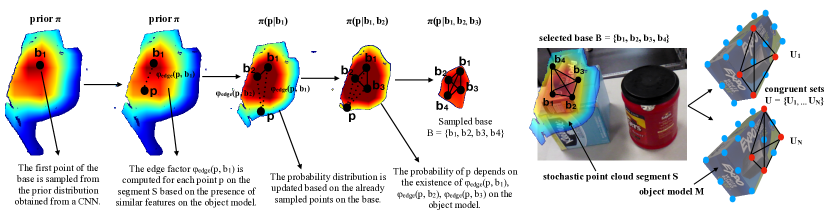
Figure 2: A description of the stochastic optimization process for extracting the base $B=\{b_{1},b_{2},b_{3},b_{4}\}$ so that it is distributed according to the stochastic segmentation and in accordance with the object’s known geometry. The base is matched against candidate sets $U=\{U_{1}$, …, $U_{N}\}$ of 4 congruent points each from the object model $M$.

3.3 Stochastic Optimization for Selecting the Base

The process for selecting the base is given in Alg. 2 and highlighted in Fig. 2. As only a limited number of bases can be evaluated in a given time frame, it is critical to ensure that all base points belong to the object in consideration with high probability. Using the Hammersley-Clifford factorization, the joint probability of points in $B=\{b_{1},b_{2},b_{3},b_{4}\mid b_{1:4}\in S_{k}\}$ belonging to $O_{k}$ is given as:

$$Pr(B\rightarrow O_{k})=\frac{1}{Z}\prod_{i=0}^{m}\phi(C_{i}),$$ (4)

where $C_{i}$ is defined as a clique in a fully-connected graph that has as nodes $b_{1},b_{2},b_{3}$ and $b_{4}$, $Z$ is the normalization constant and $\phi(C_{i})$ corresponds to the factor potential of the clique $C_{i}$. For computational efficiency, only cliques of sizes 1 and 2 are considered, which are respectively the nodes and edges in the complete graph of $\{b_{1},b_{2},b_{3},b_{4}\}$. The above simplification gives rise to the following approximation of Eqn. 4:

$$Pr(B\rightarrow O_{k})=\frac{1}{Z}\prod_{i=1}^{4}\{\phi_{node}(b_{i})\prod_{j=1}^{j<i}\phi_{edge}(b_{i},b_{j})\}.$$

The above operation is implemented efficiently in an incremental manner. The last element of the implementation is the definition of the factor potentials for nodes and edges of the graph $\{b_{1},b_{2},b_{3},b_{4}\}$. The factor potential for the nodes can be computed by using the class probabilities returned by the CNN-based soft segmentation, i.e.

$$\phi_{node}(b_{i})=\pi_{k}(b_{i}).$$

The factor potentials $\phi_{edge}$ for edges can be computed using the Point-Pair Feature (PPF) of the two points [Drost et al.(2010)Drost, Ulrich, Navab, and Ilic] defining the edge and the frequency of the computed feature on the CAD model $M_{i}$ of the object. The PPF for two points on the model $m_{1},m_{2}$ with surface normals $n_{1},n_{2}$:

$${\tt PPF}(m_{1},m_{2})=(\mid\mid d\mid\mid_{2},\angle(n_{1},d),\angle(n_{2},d),\angle(n_{1},n_{2})),$$

wherein $d=m_{2}-m_{1}$ is the vector from $m_{1}$ to $m_{2}$.

1 $b_{1}$ $\leftarrow$ sample a point from $S_{k}$ according to the discrete probability distribution defined by the soft segmentation prior $\pi_{k}$ ;

2 foreach point $p\in S_{k}$ do

3       $\pi(p|b_{1})=\pi_{k}(p)\pi_{k}(b_{1})\phi_{edge}(p,b_{1})$;

4      

5$b_{2}$ $\leftarrow$ sample from normalized $\pi(.|b_{1})$;

6 foreach point $p\in S_{k}$ do

7       $\pi(p|b_{1},b_{2})=\pi(p|b_{1})\pi(b_{2}|b_{1})\phi_{edge}(p,b_{2})$;

8       if $\angle((p-b_{0}),(b_{1}-b_{0}))<\epsilon_{1}$ then

9             $\pi(p|b_{1},b_{2})$ $\leftarrow$ 0 ;

10            

11$b_{3}$ $\leftarrow$ sample from normalized $\pi(.|b_{1},b_{2})$;

12 foreach point $p\in S_{k}$ do

13       $\pi(p|b_{1},b_{2},b_{3})=\pi(p|b_{1},b_{2})\pi(b_{3}|b_{1},b_{2})\phi_{edge}(p,b_{3})$;

14       if distance(plane($b_{1},b_{2},b_{3}$), p) $<$ $\epsilon_{2}$ then

15             $\pi(p|b_{1},b_{2},b_{3})$ $\leftarrow$ 0 ;

16            

17$b_{4}$ $\leftarrow$ sample from normalized $\pi(.|b_{1},b_{2},b_{3})$;

18 return $b_{1},b_{2},b_{3},b_{4}$;

Algorithm 2 select_StoCS_base ($S_{k}$, $\pi_{k}$, $M_{k}$)

A hash map is generated for the object model, which counts the number of occurrences of discretized point pair features in the model. To account for the sensor noise, the point pair features are discretized. Nevertheless, even with discretization, the surface normals of points in the scene point cloud could be noisy enough such that they do not map to the same bin as the corresponding points on the model. To overcome this issue, during the model generation process, each point pair also votes to several neighboring bins. For the accompanying implementation, the bin discretization was kept at 10 degrees and 0.5 cm. The point-pair features voted to $2^{4}$ other bins in the neighborhood of the bin the feature points to. This ensures the robustness of the method in case of noisy surface normal computations. Then, the factor potential for edges in the base is given as:

$$\phi_{edge}(b_{i},b_{j})=\begin{cases}1,\text{ if }hashmap(M_{k},{\tt PPF}(b_{i},b_{j}))>0\cr 0,\text{ otherwise}\end{cases}$$

Thus, the sampling of bases incorporates the above definitions and proceeds as described in Algorithm 2. In particular, each of the four points in a base $B$ is sampled from the discrete probability distribution $\pi_{k}$, defined for the point segment $S_{k}$. This distribution is initialized as shown in Eqns. 1 and  3 using the output of the last layer of a CNN. The probability of sampling a point $p\in S_{k}$ is incrementally updated in Algorithm 2 by considering the edge potentials of points with already sampled points in the base. This step essentially prunes points that do not relate, according to the geometric model of the object, to the already sampled points in the base. Furthermore, constraints are defined in the form of conservative thresholds ($\epsilon_{1}$, $\epsilon_{2}$) to ensure that the selected base has a wide interior angle and is coplanar.

The find_congruent_sets(B, $M_{k}$) subroutine of Algorithm 1 is used to compute a set $\mathcal{U}$ of 4-points from $M_{k}$ that are congruent to the sampled base B. The 4-points of the base can be represented by two pairs represented by their respective PPF and the ratio defined on the line segments by virtue of their intersection. Two sets of point pairs are computed on the model with the PPFs specified by the segment base. The pairs in the two sets, which also intersect with the given ratios are classified as congruent 4-points. The basic idea of 4 point congruent sets was originally proposed in [Aiger et al.(2008)Aiger, Mitra, and Cohen-Or]. It was derived from the fact that these ratios and distances are invariant across any rigid transformation. In StoCS the pairs are compared using point-pair features instead of just distances, which further reduces the cardinality of the sets of pairs that need to be compared and thus speed-ups the search process.

4 Evaluation

Two different datasets are used for the evaluation of the proposed method.

4.1 Amazon Picking Challenge (APC) dataset

This RGB-D dataset [Mitash et al.(2018)Mitash, Boularias, and Bekris] contains real images of multiple objects from the Amazon Picking Challenge (APC) in varying configurations involving occlusions and texture-less objects.

A Fully Convolutional Network (FCN) was trained for semantic segmentation by using synthetic data. The synthetic images were generated by a toolbox for this dataset [Mitash et al.(2017)Mitash, Bekris, and Boularias]. A dataset bias was observed, leading to performance drop on mean recall for pixel-wise prediction from 95.3% on synthetic test set to 77.9% on real images. Recall can be improved by using a continuous probability output from the FCN with no or very low confidence threshold as proposed in this work. This comes at the cost of losing precision and including parts of other objects in the segment being considered for model registration. Nevertheless, it is crucial to achieve accurate pose estimation on real images given a segmentation process trained only on synthetic data as it significantly reduces labeling effort.

Table 4.1 provides the pose accuracy of StoCS compared against Super4PCS and V4PCS. The Volumetric-4PCS (V4PCS) approach samples 4 base points by optimizing for maximum volume and thus coplanarity is no more a constraint. Congruency is established when all the edges of the tetrahedron formed by connecting the points have the same length. The performance is evaluated as mean error in translation and rotation, where the rotation error is a mean of the roll, pitch, and yaw error. The three processes sample 100 segment bases and verify all the transformations extracted from the congruent sets. While StoCS uses soft segmentation output, the segment for the competing approaches was obtained by thresholding on per-pixel class prediction probability. In Table 1(a), the optimal value of the threshold ($\epsilon=$ 0.4) is used for Super4PCS and V4PCS. In Figure 1(b), the robustness of all approaches is validated for different thresholds. The percentage of successful estimates (error less than 2cm and 10 degrees) reduces with the segmentation accuracy for both Super4PCS and V4PCS. But StoCS provides robust estimates even when the segmentation precision is very low. The StoCS output using FCN segmentation is comparable to results with registration on ground-truth segmentation, which is an ideal case for the alternative methods. This is important as it is not always trivial to compute the optimal threshold for a test scenario.

Method Rot. error Tr. error Time Super4PCS [Mellado et al.(2014)Mellado, Aiger, and Mitra] 8.83∘ 1.36cm 28.01s V4PCS [Huang et al.(2017)Huang, Kwok, and Zhou] 10.75∘ 5.48cm 4.66s StoCS (OURS) 6.29∘ 1.11cm 0.72s
(a) Average rotation error, translation error and execution time (per object)	(b) Robustness with varying segmentation confidences.

Method Base Sampling Set Extraction Set Verification #Set per base Super4PCS [Mellado et al.(2014)Mellado, Aiger, and Mitra] 0.0045s 2.43s 19.98s 1957.18 V4PCS [Huang et al.(2017)Huang, Kwok, and Zhou] 0.0048s 1.98s 0.36s 46.61 StoCS (OURS) 0.0368s 0.27s 0.37s 53.52

(c) Computation complexity for the different components of the registration process.

Table 1: Comparing StoCS with related registration processes on the APC dataset.

4.2 Computational cost

The computational cost of the process can be broken down into 3 components: base sampling, congruent set extraction, and set verification. StoCS increases the cost of base sampling as it iterates over the segment to update probabilities. But this is linear in the size of the segment and is not the dominating factor in the overall cost. The congruent set extraction and thus the verification step are output sensitive as the cost depends on the number of matching pairs on the model corresponding to 2 line segments on the sampled base for Super4PCS and StoCS and 6 line segments of the tetrahedron for V4PCS. Thus, base sampling optimizes for wide interior angle or large volume in Super4PCS and V4PCS respectively to reduce the number of similar sets on the model. This optimization, however, could lead to the selection of outlier points in the sampled base, which occurs predominantly in V4PCS. For Super4PCS  the number of congruent pairs still turns out to be very large (approx., 2000 per base), thus leading to a computationally expensive set extraction and verification stage. This is mostly seen for objects with large surfaces and symmetric objects. StoCS can restrict the number of congruent sets by only considering pairs on the model, which have the same PPF as on the sampled base. It does not optimize for wide interior angle or maximizing volume, but imposes a small threshold, such that nearby points and redundant structures are avoided in base sampling. So it can handle the computational cost without hurting accuracy as shown in Table 4.1 part (c).

4.3 YCB-Video dataset

The YCB-Video dataset [Xiang et al.(2018)Xiang, Schmidt, Narayanan, and Fox] is a benchmark for robotic manipulation tasks that provides scenes with a clutter of 21 YCB objects [Calli et al.(2017)Calli, Singh, Bruce, Walsman, Konolige, Srinivasa, Abbeel, and Dollar] captured from multiple views and annotated with 6-DOF object poses. Along with the dataset, the authors also proposed an approach, PoseCNN, which learns to predict the object center and rotation solely on RGB images. The poses are further fine-tuned by initializing a modified ICP with the output of PoseCNN, and applying it on the depth images. The metric used for pose evaluation in this benchmark measures the average distance between model points transformed using the ground truth transformation and with the predicted transform. An accuracy-threshold curve is plotted and the area under the curve is reported as a scalar representation of the accuracy for each approach. To ignore errors caused due to object symmetry, the closest symmetric point is considered as a correspondence to compute the error.

Method Pose success Time PoseCNN [Xiang et al.(2018)Xiang, Schmidt, Narayanan, and Fox] 57.37$\%$ 0.2s PoseCNN+ICP [Xiang et al.(2018)Xiang, Schmidt, Narayanan, and Fox] 76.53$\%$ 10.6s PPF-Hough [Drost et al.(2010)Drost, Ulrich, Navab, and Ilic] 83.97$\%$ 7.18s Super4PCS [Mellado et al.(2014)Mellado, Aiger, and Mitra] 87.21$\%$ 43s V4PCS [Huang et al.(2017)Huang, Kwok, and Zhou] 77.34$\%$ 4.32s StoCS (OURS) 90.1$\%$ 0.59s

Table 2: (left) Success given the area under the accuracy-threshold curve and computation time (per object) on the YCB-Video dataset. (right) Anytime results for 3 pointset registration methods.

The results of the evaluation are presented in Table 2. The accuracy of PoseCNN is low, mostly because it does not use depth information. When combined with a modified ICP, the accuracy increases but at a cost of large computation time. The modified ICP performs a gradient-descent in the depth image by generating a rendering score for hypothesized poses. The results are reported by running the publicly shared code separately over each view of the scene, which may not be optimal for the approach but is a fair comparison point as all the compared methods are tested on the same images.

For evaluating the other approaches, the same dataset used to train PoseCNN was employed to train FCN for semantic segmentation with a VGG16 architecture. A deterministic segment was computed based on thresholding over the network output. An alternative that is evaluated is Hough voting [Drost et al.(2010)Drost, Ulrich, Navab, and Ilic]. This achieves better accuracy but is computationally expensive. This is primarily due to the quadratic complexity over the points on the segment, which perform the voting. Next, alternative congruent set based approaches were evaluated, Super4PCS and V4PCS. For each approach 100 iterations of the algorithm were executed. As the training dataset was similar to the test dataset, and an optimal threshold was used, 100 iterations were enough for Super4PCS to find good pose estimates. Nevertheless, Super4PCS generates a large number of congruent sets, even when surface normals were used to prune correspondences, leading to large computation time. V4PCS achieves lower accuracy. During its base sampling process, V4PCS optimizes for maximizing volume, which often biases towards outliers.

Finally, the proposed approach was tested. A continuous soft segmentation output was used in this case, instead of optimal threshold and 100 iterations of the algorithm was run. It achieves the best accuracy, and the computation time is just slightly larger than PoseCNN which was designed for time efficiency as it uses one forward pass over the neural network.

5 Discussion

Scene segmentation and object pose estimation are two problems that are frequently addressed separately. The points provided by segmentation are generally treated with an equal level of certainty by pose estimation algorithms. This paper shows that a potentially better way is to exploit the varying levels of confidence obtained from segmentation tools, such as CNNs. This leads to a stochastic search for object poses that achieves improved pose estimation accuracy, especially in setups where the segmentation is imperfect, such as when the CNN is trained using synthetic data. This is increasingly popular for training CNNs to minimize human effort [Georgakis et al.(2016)Georgakis, Mousavian, Berg, and Kosecká].

A limitation of the proposed method is the difficulty to deal with cases where depth information is unavailable, such as with translucent objects [Phillips et al.(2017)Phillips, Lecce, and Daniilidis]. This can be addressed by sampling points on hypothesized object surfaces, instead of relying fully on points detected by depth sensors. Another extension is to generalize the pointset bases to contain arbitrary sets of points with desirable properties. For instance, determinantal point processes [Soshnikov(2000)] can be used for sampling sets of points according to their diversity.

References

- [Aiger et al.(2008)Aiger, Mitra, and Cohen-Or] D. Aiger, N. J. Mitra, and D. Cohen-Or. 4-points Congruent Sets for Robust Pairwise Surface Registration. ACM Transactions on Graphics (TOG), 27(3):85, 2008.
- [Aldoma et al.(2012)Aldoma, Marton, Tombari, Wohlkinger, Potthast, Zeisl, Rusu, Gedikli, and Vincze] A. Aldoma, Z.-C. Marton, F. Tombari, W. Wohlkinger, C. Potthast, B. Zeisl, R. B. Rusu, S. Gedikli, and M. Vincze. Tutorial: Point cloud library: Three-dimensional object recognition and 6 dof pose estimation. IEEE RAM, 19(3):80–91, 2012.
- [Ballard(1981)] Dana H Ballard. Generalizing the hough transform to detect arbitrary shapes. Pattern recognition, 13(2):111–122, 1981.
- [Besl and McKay(1992)] P. J. Besl and N. D. McKay. Method for Registration of 3D Shapes. International Society for Optics and Photonics, 1992.
- [Birdal and Ilic(2015)] Tolga Birdal and Slobodan Ilic. Point pair features based object detection and pose estimation revisited. In 3D Vision (3DV), 2015 International Conference on, pages 527–535. IEEE, 2015.
- [Bouazix et al.(2013)Bouazix, Tagliasacchi, and Pauly] S. Bouazix, A. Tagliasacchi, and M. Pauly. Sparse Iterative Closest Point. Computer Graphics Forum (Symposium on Geometry Processing), 32(5):1–11, 2013.
- [Brachmann et al.(2014)Brachmann, Krull, Michel, Gumhold, Shotton, and Rother] Eric Brachmann, Alexander Krull, Frank Michel, Stefan Gumhold, Jamie Shotton, and Carsten Rother. Learning 6d object pose estimation using 3d object coordinates. In European conference on computer vision, pages 536–551. Springer, 2014.
- [Calli et al.(2017)Calli, Singh, Bruce, Walsman, Konolige, Srinivasa, Abbeel, and Dollar] Berk Calli, Arjun Singh, James Bruce, Aaron Walsman, Kurt Konolige, Siddhartha Srinivasa, Pieter Abbeel, and Aaron M Dollar. Yale-cmu-berkeley dataset for robotic manipulation research. The International Journal of Robotics Research, 36(3):261–268, 2017.
- [Cheng et al.(2013)Cheng, Chen, Martin, Lai, and Wang] Z.-Q. Cheng, Y. Chen, R. Martin, Y.-K. Lai, and A. Wang. Supermatching: Feature Matching using Supersymmetric Geometric Constraints. In IEEE TVCG, volume 19, page 11, 2013.
- [Choi and Christensen(2012)] Changhyun Choi and Henrik I Christensen. 3d pose estimation of daily objects using an rgb-d camera. In Intelligent Robots and Systems (IROS), 2012 IEEE/RSJ International Conference on, pages 3342–3349. IEEE, 2012.
- [Collet et al.(2011)Collet, Martinez, and Srinivasa] A. Collet, M. Martinez, and S. Srinivasa. The MOPED framework: Object Recognition and Pose Estimation for Manipulation. International Journal of Robotics Research (IJRR), 30(10):1284–1306, 2011.
- [Correll et al.(2016)Correll, Bekris, Berenson, Brock, Causo, Hauser, Osada, Rodriguez, Romano, and Wurman] N. Correll, K. E. Bekris, D. Berenson, O. Brock, A. Causo, K. Hauser, K. Osada, A. Rodriguez, J. Romano, and P. Wurman. Analysis and Observations From the First Amazon Picking Challenge. IEEE Trans. on Automation Science and Engineering (T-ASE), 2016.
- [Drost and Ilic(2012)] B. Drost and S. Ilic. 3D Object Detection and Localization using Multimodal Point Pair Features. In Second International Conference on 3D Imaging, Modeling, Processing, Visualization and Transmission (3DIMPVT), pages 9–16, 2012.
- [Drost et al.(2010)Drost, Ulrich, Navab, and Ilic] B. Drost, M. Ulrich, N. Navab, and S. Ilic. Model Globally, Match Locally: Efficient and Robust 3D Object Recognition. In IEEE Conference on Computer Vision and Pattern Recognition (CVPR), pages 998–1005, 2010.
- [Fischler and Bolles(1981)] Martin A Fischler and Robert C Bolles. Random sample consensus: a paradigm for model fitting with applications to image analysis and automated cartography. Communications of the ACM, 24(6):381–395, 1981.
- [Gelfand et al.(2005)Gelfand, Mitra, Guibas, and Pottmann] N. Gelfand, N. Mitra, L. Guibas, and H. Pottmann. Robust Global Registration. In Proc. of the Third Eurographics Symposium on Geometry Processing, 2005.
- [Georgakis et al.(2016)Georgakis, Mousavian, Berg, and Kosecká] G. Georgakis, A. Mousavian, A. C. Berg, and J. Kosecká. Synthesizing Training Data for Object Detection in Indoor Scenes. In Robotics: Science and Systems, 2016.
- [Hernandez et al.(2016)Hernandez, Bharatheesha, Ko, Gaiser, Tan, van Deurzen, de Vries, Van Mil, van Egmond, Burger, et al.] Carlos Hernandez, Mukunda Bharatheesha, Wilson Ko, Hans Gaiser, Jethro Tan, Kanter van Deurzen, Maarten de Vries, Bas Van Mil, Jeff van Egmond, Ruben Burger, et al. Team delft’s robot winner of the amazon picking challenge 2016. In Robot World Cup, pages 613–624. Springer, 2016.
- [Hinterstoisser et al.(2012a)Hinterstoisser, Cagniart, Ilic, Sturm, Navab, Fua, and Lepetit] S. Hinterstoisser, C. Cagniart, S. Ilic, P. Sturm, N. Navab, P. Fua, and V. Lepetit. Gradient Response Maps for Real-time Detection of Textureless Objects. IEEE Transactions on Pattern Analysis and Machine Intelligence (TPAMI), 34(5):876–888, 2012a.
- [Hinterstoisser et al.(2012b)Hinterstoisser, Lepetit, Ilic, Holzer, Bradski, Konolige, and Navab] Stefan Hinterstoisser, Vincent Lepetit, Slobodan Ilic, Stefan Holzer, Gary Bradski, Kurt Konolige, and Nassir Navab. Model based training, detection and pose estimation of texture-less 3D objects in heavily cluttered scenes. In Asian Conference on Computer Vision, pages 548–562. Springer, 2012b.
- [Hinterstoisser et al.(2016)Hinterstoisser, Lepetit, Rajkumar, and Konolige] Stefan Hinterstoisser, Vincent Lepetit, Naresh Rajkumar, and Kurt Konolige. Going further with point pair features. In European Conference on Computer Vision, pages 834–848. Springer, 2016.
- [Huang et al.(2017)Huang, Kwok, and Zhou] Jida Huang, Tsz-Ho Kwok, and Chi Zhou. V4pcs: Volumetric 4pcs algorithm for global registration. Journal of Mechanical Design, 139(11):111403, 2017.
- [Irani and Raghavan(1996)] S. Irani and P. Raghavan. Combinatorial and Experimental Results for Randomized Point Matching Algorithms. In Proc. of the Symposium on Computational Geometry, pages 68–77, 1996.
- [Johnson and Hebert(1999)] Andrew E. Johnson and Martial Hebert. Using spin images for efficient object recognition in cluttered 3d scenes. IEEE Transactions on pattern analysis and machine intelligence, 21(5):433–449, 1999.
- [Kehl et al.(2017)Kehl, Manhardt, Tombari, Ilic, and Navab] Wadim Kehl, Fabian Manhardt, Federico Tombari, Slobodan Ilic, and Nassir Navab. Ssd-6d: Making rgb-based 3d detection and 6d pose estimation great again. In IEEE Conference on Computer Vision and Pattern Recognition (CVPR), pages 1521–1529, 2017.
- [Kim and Medioni(2011)] Eunyoung Kim and Gerard Medioni. 3d object recognition in range images using visibility context. In Intelligent Robots and Systems (IROS), 2011 IEEE/RSJ International Conference on, pages 3800–3807. IEEE, 2011.
- [Krull et al.(2015)Krull, Brachmann, Michel, Ying Yang, Gumhold, and Rother] Alexander Krull, Eric Brachmann, Frank Michel, Michael Ying Yang, Stefan Gumhold, and Carsten Rother. Learning analysis-by-synthesis for 6d pose estimation in rgb-d images. In Proceedings of the IEEE International Conference on Computer Vision, pages 954–962, 2015.
- [Long et al.(2015)Long, Shelhamer, and Darrell] Jonathan Long, Evan Shelhamer, and Trevor Darrell. Fully convolutional networks for semantic segmentation. In IEEE Conf. on Computer Vision and Pattern Recognition, pages 3431–3440, 2015.
- [Lowe(1999)] D. G. Lowe. Object Recognition from Local Scale-Invariant Features. In IEEE International Conference on Computer Vision (ICCV), volume 2, pages 1150–1157, 1999.
- [Mellado et al.(2014)Mellado, Aiger, and Mitra] N. Mellado, D. Aiger, and N. J. Mitra. Super4PCS Fast Global Pointcloud Registration via Smart Indexing. Computer Graphics Forum, 33(5):205–215, 2014.
- [Michel et al.(2017)Michel, Kirillov, Brachmann, Krull, Gumhold, Savchynskyy, and Rother] Frank Michel, Alexander Kirillov, Eric Brachmann, Alexander Krull, Stefan Gumhold, Bogdan Savchynskyy, and Carsten Rother. Global hypothesis generation for 6d object pose estimation. In Proceedings of the IEEE Conference on Computer Vision and Pattern Recognition, pages 462–471, 2017.
- [Mitash et al.(2017)Mitash, Bekris, and Boularias] Chaitanya Mitash, Kostas E Bekris, and Abdeslam Boularias. A self-supervised learning system for object detection using physics simulation and multi-view pose estimation. In Intelligent Robots and Systems (IROS), 2017 IEEE/RSJ International Conference on, pages 545–551. IEEE, 2017.
- [Mitash et al.(2018)Mitash, Boularias, and Bekris] Chaitanya Mitash, Abdeslam Boularias, and Kostas E Bekris. Improving 6d pose estimation of objects in clutter via physics-aware monte carlo tree search. In IEEE International Conference on Robotics and Automation (ICRA), 2018.
- [Mitra et al.(2004)Mitra, Gelfand, Pottmann, and Guibas] N. Mitra, N. Gelfand, H. Pottmann, and H. Guibas. Registration of Point Cloud Data from a Geometric Optimization Perspective. In Proc. of the 2004 Eurographics/ACM SIGGRAPH Symposium on Geometry Processing, pages 22–31, 2004.
- [Narayanan and Likhachev(2016)] V. Narayanan and M. Likhachev. Discriminatively-guided Deliberative Perceptino for Pose Estimation of Multiple 3D Object Instances. In Robotics: Science and Systems, 2016.
- [Phillips et al.(2017)Phillips, Lecce, and Daniilidis] C. J. Phillips, M. Lecce, and K. Daniilidis. Seeing Glassware: from Edge Detection to Pose Estimation and Shapre Recovery. In Robotics: Science and Systems, 2017.
- [Ren et al.(2015)Ren, He, Girshick, and Sun] Shaoqing Ren, Kaiming He, Ross Girshick, and Jian Sun. Faster r-cnn: Towards real-time object detection with region proposal networks. In Advances in Neural Information Processing Systems, pages 91–99, 2015.
- [Rothganger et al.(2006)Rothganger, Lazebnik, Schmid, and Ponce] F. Rothganger, S. Lazebnik, C. Schmid, and J. Ponce. 3D Object Modeling and Recognition using Local Affine-Invariant Image Descriptors and Multi-view Spatial Constraints. International Journal of Computer Vision (IJCV), 66(3):231–259, 2006.
- [Rusinkiewicz and Levoy(2001)] S. Rusinkiewicz and M. Levoy. Efficient Variants of the ICP Algorithm. In IEEE Proc. of 3DIM, pages 145–152, 2001.
- [Rusu et al.(2009)Rusu, Blodow, and Beetz] Radu Bogdan Rusu, Nico Blodow, and Michael Beetz. Fast point feature histograms (fpfh) for 3d registration. In Robotics and Automation, 2009. ICRA’09. IEEE International Conference on, pages 3212–3217. IEEE, 2009.
- [Segal et al.(2009)Segal, Haehnel, and Thrun] A. Segal, D. Haehnel, and S. Thrun. Generalized-ICP. In Robotics: Science and Systems, volume 2, page 4, 2009.
- [Soshnikov(2000)] A. Soshnikov. Determinantal Random Point Fields. Russian Mathematical Surveys, 55(5):932–975, 2000.
- [Srivatsan et al.(2017)Srivatsan, Vagdargi, and Choset] R. A. Srivatsan, P. Vagdargi, and H. Choset. Sparse Point Registration. In International Symposium on Robotics Research (ISRR), 2017.
- [Tejani et al.(2014)Tejani, Tang, Kouskouridas, and Kim] A. Tejani, D. Tang, R. Kouskouridas, and T. K. Kim. Latent-class Hough Forests for 3D Object Detection and Pose Estimation. In European Conference on Computer Vision, 2014.
- [Tombari et al.(2010)Tombari, Salti, and Di Stefano] Federico Tombari, Samuele Salti, and Luigi Di Stefano. Unique signatures of histograms for local surface description. In European conference on computer vision, pages 356–369. Springer, 2010.
- [Xiang et al.(2018)Xiang, Schmidt, Narayanan, and Fox] Yu Xiang, Tanner Schmidt, Venkatraman Narayanan, and Dieter Fox. PoseCNN: A Convolutional Neural Network for 6D Object Pose Estimation in Cluttered Scenes. In Robotics: Science and Systems, 2018.
- [Zeng et al.(2017)Zeng, Yu, Song, Suo, Walker Jr, Rodriguez, and Xiao] A. Zeng, K.-T. Yu, S. Song, D. Suo, E. Walker Jr, A. Rodriguez, and J. Xiao. Multi-view self-supervised deep learning for 6d pose estimation in the amazon picking challenge. In IEEE International Conference on Robotics and Automation (ICRA), 2017.