On the Application of Danskin’s Theorem to Derivative-Free Minimax Optimization

Abstract.

Motivated by Danskin’s theorem, gradient-based methods have been applied with empirical success to solve minimax problems that involve non-convex outer minimization and non-concave inner maximization. On the other hand, recent work has demonstrated that Evolution Strategies (ES) algorithms are stochastic gradient approximators that seek robust solutions. In this paper, we address black-box (gradient-free) minimax problems that have long been tackled in a coevolutionary setup. To this end and guaranteed by Danskin’s theorem, we employ ES as a stochastic estimator for the descent direction. The proposed approach is validated on a collection of black-box minimax problems. Based on our experiments, our method’s performance is comparable with its coevolutionary counterparts and favorable for high-dimensional problems. Its efficacy is demonstrated on a real-world application.

1. Introduction

Many real-world applications involve an adversary and/or uncertainty, specifically in the security domain. Consequently, several methods have been proposed to find solutions that have the best worst-case (or average) performance for security-critical systems. Important examples include face recognition (Sharif et al., 2017) and malware detection (Huang et al., 2018).

The notion of security and adversarial robustness can be described by a minimax formulation (Huang et al., 2015; Madry et al., 2017). The formulation is motivated by theoretical guarantees from Danskin’s theorem (Danskin, 1966) on using first-order information, i.e. gradients, to find or approximate solutions. Further, where theoretical guarantees can not be assumed, empirical solutions to problems, e.g. digit recognition, have been demonstrated (Madry et al., 2017).

In this paper, our interest is in black-box (gradient-free) minimax problems where, in contrast to the aforementioned examples of image recognition and malware, gradients are neither symbolically nor numerically available, or they are complex to compute (Conn et al., 2009). This has led to extensive use of coevolutionary frameworks (Herrmann, 1999; Jensen, 2001) to solve such problems. These frameworks however do not reconcile the guarantees provided by gradient-based frameworks in solving the minimax problem. Our goal is to bridge this divide and develop a method for black-box minimax that is consistent with the theoretical assumptions and guarantees of Danskin’s theorem while using a gradient estimator in lieu of a gradient. For gradient estimation, we propose to employ a class of black-box optimization algorithms, viz. Evolution Strategies (ES).

Our proposition is motivated by the growing body of work (Salimans et al., 2017; Morse et al., 2016) which has shown that the performance of gradient-based methods can be rivaled by ES, and that ES is more than just a traditional finite difference approximator (Lehman et al., 2017). For more empirical and theoretical insights on ES vs. gradient-based methods, see (Ollivier et al., 2017; Wierstra et al., 2014; Akimoto, 2012).

We report the following contributions: 1) We present a formal theoretical motivation for using ES to meet the theoretical guarantees of using gradients for gradient-free minimax problems. 2) We present the Reckless framework, which employs ES to solve black-box minimax problems that have long been addressed in a coevolutionary setup. 3) We compare variants of ES that have different properties in terms of their gradient estimation on a collection of benchmark problems. Coevolutionary approaches have often been evaluated based on the Euclidean error of their solutions with respect to the optimal solutions. Our comparison is based on the notion of regret (loss) in the objective function value at a solution with respect to that at an optimal solution. 4) We validate the effectiveness of the proposed framework and compare its performance in terms of regret against the state of the art coevolutionary algorithms on benchmark problems as well as a real-world application. We find that Reckless scales better than the majority of its coevolutionary counterparts. 5) Finally, we provide the Reckless framework and experiment code for public use.

2. Background

This section introduces the notation and terminology used in the rest of the paper, followed by a summary of coevolutionary approaches for black-box minimax problems.

2.1. Black-Box Minimax Problem

Formally, we are concerned with the black-box minimax optimization problem given a finite budget of function evaluations. Mathematically, the problem is a composition of an inner maximization problem and an outer minimization problem,

(1) $$\min_{\mathbf{x}\in\mathcal{X}}\max_{\mathbf{y}\in\mathcal{Y}}\mathcal{L}(\mathbf{x},\mathbf{y})\;,$$

where $\mathcal{X}\subseteq\mathbb{R}^{n_{x}}$, $\mathcal{Y}\subseteq\mathbb{R}^{n_{y}}$, and $\mathcal{L}:\mathcal{X}\times\mathcal{Y}\to\mathbb{R}$. The problem is called black-box because there is no closed-form expression of $\mathcal{L}$. Instead, one can query an oracle (e.g., a simulation) for the value of $\mathcal{L}$ at a specific pair $(\mathbf{x},\mathbf{y})\in\mathcal{X}\times\mathcal{Y}$. The task is then to find the optimal solution $\mathbf{x}^{*}\in\mathcal{X}$ to Eq. 1, whose corresponding objective function value $\mathcal{L}(\mathbf{x}^{*},\cdot)$ is at its max at $\mathbf{y}^{*}\in\mathcal{Y}$, or a good approximate using a finite number of function evaluations, which are expensive in terms of computational resources (e.g. CPU time).

The pair $(\hat{\mathbf{x}},\hat{\mathbf{y}})\in\mathcal{X}\times\mathcal{Y}$ is called a saddle point of Eq. 1 if $\forall\mathbf{x}\in\mathcal{X}$, $\forall\mathbf{y}\in\mathcal{Y}$,

(2) $$\mathcal{L}(\hat{\mathbf{x}},\mathbf{y})\leq\mathcal{L}(\hat{\mathbf{x}},\hat{\mathbf{y}})\leq\mathcal{L}(\mathbf{x},\hat{\mathbf{y}})\;.$$

Equivalently (Jensen, 2001), such pair exists if:

(3) $$\min_{\mathbf{x}\in\mathcal{X}}\max_{\mathbf{y}\in\mathcal{Y}}\mathcal{L}(\mathbf{x},\mathbf{y})=\max_{\mathbf{y}\in\mathcal{Y}}\min_{\mathbf{x}\in\mathcal{X}}\mathcal{L}(\mathbf{x},\mathbf{y})\;.$$

If a saddle point exists, then it follows from Eq. 2, that

(4) $$\min_{\mathbf{x}\in\mathcal{X}}\max_{\mathbf{y}\in\mathcal{Y}}\mathcal{L}(\mathbf{x},\mathbf{y})=max_{\mathbf{y}\in\mathcal{X}}\mathcal{L}(\hat{\mathbf{x}},\mathbf{y})=min_{\mathbf{x}\in\mathcal{X}}\mathcal{L}(\mathbf{x},\hat{\mathbf{y}})\;.$$

From a game theory perspective, a saddle point represents a two-player zero-sum game equilibrium. Minimax problems with saddle points are referred to as symmetrical problems (Jensen, 2003), in contrast to asymmetrical problems for which the condition Eq. 2 does not hold.

Given an algorithm’s best solution $\mathbf{x}_{*}$ to Eq. 1, the mean square Euclidean error (MSE) has been used as a performance metric to compare $\mathbf{x}_{*}$ to the optimal solution $\mathbf{x}^{*}$ (Qiu et al., 2017; Cramer et al., 2009). That is,

(5) $$\text{MSE}(\mathbf{x}_{*})=\frac{1}{n_{x}}||\mathbf{x}_{*}-\mathbf{x}^{*}||^{2}_{2}\;.$$

In this paper, we introduce a metric that is closely related to the notion of loss in decision-making problems under adversary and/or uncertainty as well as continuous optimization (Bubeck et al., 2012; Valko et al., 2013): the regret of an algorithm’s best solution $\mathbf{x}_{*}$ in comparison to the optimal solution $\mathbf{x}^{*}$ is defined as

(6) $$r(\mathbf{x}_{*})=\max_{\mathbf{y}\in\mathcal{Y}}\mathcal{L}(\mathbf{x}_{*},\mathbf{y})-\mathcal{L}(\mathbf{x}^{*},\mathbf{y}^{*})\;,$$

where the first term can be computed using an ensemble of off-the-shelf black-box continuous optimization solvers. Note that the regret measure, in comparison to MSE, allows us to compare the quality of several proposed solutions without the knowledge about the pair $(\mathbf{x}^{*},\mathbf{y}^{*})$ by just computing the first term of Eq. 6.

Algorithm 1 Coevolutionary Algorithm Alternating (CoevA)
Input:
       $T$: number of iterations,        $\tau$ : tournament size,
       $\mu$: mutation probability,        $\lambda$ : population size

1:$\mathbf{x}_{1,0},\ldots,\mathbf{x}_{\lambda,0}\sim\mathcal{U}(\mathcal{X})$

2:$\mathbf{y}_{1,0},\ldots,\mathbf{y}_{\lambda,0}\sim\mathcal{U}(\mathcal{Y})$

3:$\mathbf{X}_{0}\leftarrow[\mathbf{x}_{1,0},\ldots,\mathbf{x}_{\lambda,0}]$$\triangleright$ Initialize minimizer population

4:$\mathbf{Y}_{0}\leftarrow[\mathbf{y}_{1,0},\ldots,\mathbf{y}_{\lambda,0}]$$\triangleright$ Initialize maximizer population

5:$t\leftarrow 0$

6:repeat

7:    sort($\mathbf{X}_{t},\mathcal{L}$)

8:    sort($\mathbf{Y}_{t},\mathcal{L}$)

9:    $t\leftarrow t+1$ $\triangleright$ Increase counter

10:    $\mathbf{X}_{t}\leftarrow$ select from $s(\mathbf{X}_{t-1},\tau)$ $\triangleright$ Tournament selection

11:    $\mathbf{X}_{t}\leftarrow$ perturb values in $m(\mathbf{X}_{t},\mu)$ $\triangleright$ Gaussian mutation

12:    $\mathbf{x}^{\prime}_{*},\mathbf{y}^{\prime}_{*}\leftarrow\arg\min_{\mathbf{x}\in\mathbf{X}_{t}}\arg\max_{\mathbf{y}\in\mathbf{Y}_{t-1}}\mathcal{L}(\mathbf{x},\mathbf{y})$ $\triangleright$ Best minimizer

13:    if $\mathcal{L}(\mathbf{x}^{\prime}_{*},\mathbf{y}^{\prime}_{*})<\mathcal{L}(\mathbf{x}_{\lambda,t-1},\mathbf{y}_{\lambda,t-1})$ then $\triangleright$ Replace worst minimizer

14:         $\mathbf{x}_{\lambda,t-1}\leftarrow\mathbf{x}^{\prime}_{*}$ $\triangleright$ Update population

15:    end if

16:    $\mathbf{X}_{t}\leftarrow\mathbf{X}_{t-1}$ $\triangleright$ Replicate population

17:    $t\leftarrow t+1$ $\triangleright$ Increase counter before alternating

18:    $\mathbf{Y}_{t}\leftarrow$ select from $s(\mathbf{Y}_{t-1},\tau)$ $\triangleright$ Tournament selection

19:    $\mathbf{Y}_{t}\leftarrow$ perturb values with $m(\mathbf{Y}_{t},\mu)$ $\triangleright$ Gaussian mutation

20:    $\mathbf{x}^{\prime}_{0},\mathbf{y}^{\prime}_{0}\leftarrow\arg\min_{\mathbf{x}\in\mathbf{X}_{t}}\arg\max_{\mathbf{y}\in\mathbf{Y}_{t}}\mathcal{L}(\mathbf{x},\mathbf{y})$ $\triangleright$ Best maximizer

21:    if $\mathcal{L}(\mathbf{x}^{\prime}_{0},\mathbf{y}^{\prime}_{0})>\mathcal{L}(\mathbf{x}_{\lambda,t},\mathbf{y}_{\lambda,t-1})$ then $\triangleright$ Replace worst maximizer

22:         $\mathbf{y}_{\lambda,t-1}\leftarrow\mathbf{y}^{\prime}_{0}$ $\triangleright$ Update population

23:    end if

24:    $\mathbf{Y}_{t}\leftarrow\mathbf{Y}_{t-1}$ $\triangleright$ Replicate population

25:until $t\geq T$

26:$\mathbf{x}_{*},\mathbf{y}_{*}\leftarrow\arg\min_{\mathbf{x}\in\mathbf{X}_{T}}\arg\max_{\mathbf{y}\in\mathbf{Y}_{T}}\mathcal{L}(\mathbf{x},\mathbf{y})$ $\triangleright$ Best minimizer

27:return $\mathbf{x}_{*},\mathbf{y}_{*}$

2.2. Coevolutionary Approaches

Coevolutionary algorithms for minmax problems maintain two populations, the first respresents solutions and the second contains tests(Herrmann, 1999). The fitness of solution is determined by its performance when it interacts with some set of tests. In this work, we explore two variants of this approach - alternating and parallel. In alternating, the two populations (one for finding the minimum, and one for the maximum) take turns in evolving, learning from the previous iteration’s population. In parallel, the updates to both the populations happen in each step. Ideally there is convergence to a robust solution and its worst-case tests. The algorithms for these two approaches are listed in Algorithm  1 and 2, see (Bäck et al., 2000) for selection and mutation operator details.

Algorithm 2 Coevolutionary Algorithm Parallel (CoevP)
Input:
       $T$: number of iterations,        $\tau$ : tournament size,
       $\mu$: mutation probability,        $\lambda$ : population size

1:$\mathbf{x}_{1,0},\ldots,\mathbf{x}_{\lambda,0}\sim\mathcal{U}(\mathcal{X})$

2:$\mathbf{y}_{1,0},\ldots,\mathbf{y}_{\lambda,0}\sim\mathcal{U}(\mathcal{Y})$

3:$\mathbf{X}_{0}\leftarrow[\mathbf{x}_{1,0},\ldots,\mathbf{x}_{\lambda,0}]$$\triangleright$ Initialize minimizer population

4:$\mathbf{Y}_{0}\leftarrow[\mathbf{y}_{1,0},\ldots,\mathbf{y}_{\lambda,0}]$$\triangleright$ Initialize maximizer population

5:$t\leftarrow 0$

6:repeat

7:    sort($\mathbf{X}_{t},\mathcal{L}$)

8:    sort($\mathbf{Y}_{t},\mathcal{L}$)

9:    $t\leftarrow t+1$ $\triangleright$ Increase counter

10:    $\mathbf{X}\leftarrow$ select from $s(\mathbf{X}_{t-1},\tau)$ $\triangleright$ Tournament selection

11:    $\mathbf{Y}\leftarrow$ select from $s(\mathbf{Y}_{t-1},\tau)$ $\triangleright$ Tournament selection

12:    $\mathbf{X}\leftarrow$ perturb values with $m(\mathbf{X},\mu)$ $\triangleright$ Gaussian mutation

13:    $\mathbf{Y}\leftarrow$ perturb values with $m(\mathbf{Y},\mu)$ $\triangleright$ Gaussian mutation

14:    $\mathbf{x}^{\prime}_{*},\mathbf{y}^{\prime}_{*}\leftarrow\arg\min_{\mathbf{x}\in\mathbf{X}}\arg\max_{\mathbf{y}\in\mathbf{Y}}\mathcal{L}(\mathbf{x},\mathbf{y})$ $\triangleright$ Best minimizer

15:    if $\mathcal{L}(\mathbf{x}^{\prime}_{*},\mathbf{y}^{\prime}_{*})<\mathcal{L}(\mathbf{x}_{\lambda,t-1},\mathbf{y}_{\lambda,t-1})$ then $\triangleright$ Replace worst minimizer

16:         $\mathbf{x}_{\lambda,t-1}\leftarrow\mathbf{x}^{\prime}_{*}$ $\triangleright$ Update population

17:    end if

18:    $\mathbf{x}^{\prime}_{0},\mathbf{y}^{\prime}_{0}\leftarrow\arg\min_{\mathbf{x}\in\mathbf{X}}\arg\max_{\mathbf{y}\in\mathbf{Y}}\mathcal{L}(\mathbf{x},\mathbf{y})$ $\triangleright$ Best maximizer

19:    if $\mathcal{L}(\mathbf{x}^{\prime}_{0},\mathbf{y}^{\prime}_{0})>\mathcal{L}(\mathbf{x}_{\lambda,t-1},\mathbf{y}_{\lambda,t-1})$ then $\triangleright$ Replace worst maximizer

20:         $\mathbf{y}_{\lambda,t-1}\leftarrow\mathbf{y}^{\prime}_{0}$ $\triangleright$ Update population

21:    end if

22:    $\mathbf{X}_{t}\leftarrow\mathbf{X}_{t-1}$ $\triangleright$ Replace population

23:    $\mathbf{Y}_{t}\leftarrow\mathbf{Y}_{t-1}$ $\triangleright$ Replace population

24:until $t\geq T$

25:$\mathbf{x}_{*},\mathbf{y}_{*}\leftarrow\arg\min_{\mathbf{x}\in\mathbf{X}_{T}}\arg\max_{\mathbf{y}\in\mathbf{Y}_{T}}\mathcal{L}(\mathbf{x},\mathbf{y})$ $\triangleright$ Best minimizer

26:return $\mathbf{x}_{*},\mathbf{y}_{*}$

Minimax Differential Evolution (MMDE)

The MMDE algorithm introduced by Qiu et al. (2017) attempts to overcome the limitations of existing approaches in solving minimax optimization problems using differential evolution. They introduce a bottom-boosting scheme which skips redundant objective function computations while maintaining the reliability of solution evaluations. Their approach finds solutions with the best worst-case performance rather than computing worst-case scenarios for all the candidates. They realize this insight by modeling their population space as a min-heap. Although they motivate the problem well, their solution is not driven by any theoretical insight.

3. Methods

In this section, we present our proposed framework to use ES for black-box minimax problems after providing a formal motivation for the same.

ES are heuristic search methods inspired by natural evolution. Given a fitness (objective) function, say $f:\mathcal{X}\to\mathbb{R}$, these methods mutate (perturb) a population of genotypes (search points in $\mathcal{X}$) over multiple generations (iterations). At each generation, the fitness of each genotype is evaluated based on $f$. The fittest genotypes among the current population are then recombined to generate the next population. At the end, the genotype (corresponds to a point in $\mathcal{X}$) with the best fitness value is returned as the best point that optimizes $f$. The notion of ”best” refers to the minimum or maximum obtained value of $f$ in a minimization or maximization setup, respectively. Here, we briefly describe one form of ES, in particular a simplified version of natural ES that has recently gained significant attention by the machine learning community (Lehman et al., 2017). As outlined in Algorithm 3, it represents the population with an isotropic Gaussian distribution over the search space $\mathcal{X}$ with mean $\bm{\mu}$ and fixed covariance $\sigma^{2}I$ where $I$ is the identity matrix. Over generations, the algorithm aims to maximize the expected fitness value $\mathbb{E}_{\mathbf{x}\sim\mathcal{N}(\bm{\mu},\sigma^{2}I)}[f(\mathbf{x})]$ with respect to the distribution’s mean $\bm{\mu}$ via stochastic gradient ascent using a population size of $\lambda$ as shown in Line 7 of Algorithm 3, which makes use of the re-parameterization and log-likelihood tricks with $\mathbf{x}=\bm{\mu}+\sigma\bm{\epsilon}$ (Wierstra et al., 2014; Salimans et al., 2017).:

$$\mathbb{E}_{\mathbf{x}\sim\mathcal{N}(\bm{\mu},\sigma^{2}I)}[f(\mathbf{x})]=\mathbb{E}_{\bm{\epsilon}\sim\mathcal{N}(0,I)}[f(\bm{\mu}+\sigma\bm{\epsilon})]$$

(7) $$\nabla_{\bm{\mu}}\mathbb{E}_{\mathbf{x}\sim\mathcal{N}(\bm{\mu},\sigma^{2}I)}[f(\mathbf{x})]=\frac{1}{\sigma}\mathbb{E}_{\bm{\epsilon}\sim\mathcal{N}(0,I)}[f(\bm{\mu}+\sigma\bm{\epsilon})\bm{\epsilon}]$$

Algorithm 3 A Simplified Example of Evolution Strategy (ES)
Input:
       $\eta$ : learning rate
$\sigma$ : perturbation standard deviation,
$\lambda$ : number of perturbations (population size)
       $T$ : number of iterations (generations),
$f:\mathcal{X}\to\mathbb{R}$ : fitness function

1:${\bm{\mu}}_{0}\sim\mathcal{U}(\mathcal{X})$

2:for $t=0$ to $T$ do

3:    for $i=1$ to $\lambda$ do

4:         $\bm{\epsilon}_{i}\sim\mathcal{N}(0,I)$

5:         $f_{i}\leftarrow f(\bm{\mu}_{t}+\sigma\bm{\epsilon}_{i})$

6:    end for

7:    $\bm{\mu}_{t+1}\leftarrow\bm{\mu}_{t}+\eta\frac{1}{\lambda\sigma}\sum_{i=1}^{\lambda}f_{i}\bm{\epsilon}_{i}$

8:end for

Descent Direction for Minimax

Next, we show that the direction computed by the random perturbations of the current mean (Line 7 of Algorithm 3) can be used to approximate a descent direction of $\max_{\mathbf{y}}\mathcal{L}(\mathbf{x},\mathbf{y})$. Prior to that and for completeness, we reproduce (Madry et al., 2017)’s proposition A.2 on the application of Danskin’s theorem (Danskin, 1966) for minimax problems that are continuously differentiable in $\mathbf{x}$.

Theorem 3.1 (Madry et al. (2017)).

Let $\mathbf{y}^{*}$ be such that $\mathbf{y}^{*}\in\mathcal{Y}$ and is a maximizer for$\;\max_{\mathbf{y}}\mathcal{L}(\mathbf{x},\mathbf{y})$. Then, as long as it is nonzero, $-\nabla_{\mathbf{x}}\mathcal{L}(\mathbf{x},\mathbf{y}^{*})$ is a descent direction for $\;\max_{\mathbf{y}}\mathcal{L}(\mathbf{x},\mathbf{y})$.

Proof.

See (Madry et al., 2017). ∎

From Theorem 3.1 and the assumption that $L$ is twice continuously differentiable in $\mathbf{x}$, we have the following corollary.

Corollary 3.2.

Let $\mathbf{y}^{*}$ be such that $\mathbf{y}^{*}\in\mathcal{Y}$ and is a maximizer for$\;\max_{\mathbf{y}}\mathcal{L}(\mathbf{x},\mathbf{y})$. Then, for an arbitrary small $\sigma>0$ and $\mathbf{\epsilon}_{1},\ldots,\mathbf{\epsilon}_{\lambda}\sim\mathcal{N}(0,I)$,

(8) $$-\frac{1}{\sigma\lambda}\sum^{\lambda}_{i=1}\mathcal{L}(\mathbf{x}+\sigma\mathbf{\epsilon}_{i},\mathbf{y}^{*})\mathbf{\epsilon}_{i}$$

is a Monte Carlo approximation of a descent direction for$\;\max_{\mathbf{y}}\mathcal{L}(\mathbf{x},\mathbf{y})$.

Proof.

Without loss of generality, let $\mathcal{X}\subseteq\mathbb{R}$. Then, since $\sigma$ is arbitrary small, we can approximate $\mathcal{L}$ with a second-order Taylor polynomial,

(9) $$\mathcal{L}(x+{\sigma\epsilon},\mathbf{y}^{*})\approx\mathcal{L}(x,\mathbf{y}^{*})+\mathcal{L}^{\prime}(x,\mathbf{y}^{*})\sigma\epsilon+\frac{1}{2}\mathcal{L}^{\prime\prime}(x,\mathbf{y}^{*})\sigma^{2}\epsilon^{2}\;.$$

Based on Eq. 9 and the linearity of expectation, the expectation of $\mathcal{L}(x+\sigma\epsilon,\mathbf{y}^{*})\epsilon$ with respect to $\epsilon\sim\mathcal{N}(0,1)$, $\mathbb{E}_{\epsilon}[\mathcal{L}(x+\sigma\epsilon,\mathbf{y}^{*})\epsilon]$, can be written as

(10) $$\underbrace{\mathbb{E}_{\epsilon}[\mathcal{L}(x,\mathbf{y}^{*})\epsilon]}_{0}+\underbrace{\mathbb{E}_{\epsilon}[\mathcal{L}^{\prime}(x,\mathbf{y}^{*})\sigma\epsilon^{2}]}_{\mathcal{L}^{\prime}(x,\mathbf{y}^{*})\sigma}+\frac{1}{2}\underbrace{\mathbb{E}_{\epsilon}[\mathcal{L}^{\prime\prime}(x,\mathbf{y}^{*})\sigma^{2}\epsilon^{3}]}_{0}\;,$$

where the values of the terms (written under the corresponding braces) come from the definition of central moments of the Gaussian distribution (Winkelbauer, 2012). That is, $\mathbb{E}_{\epsilon}[\mathcal{L}(x+\epsilon,\mathbf{y}^{*})\epsilon]\approx\mathcal{L}^{\prime}(x,\mathbf{y}^{*})\sigma$. Thus, $-\mathcal{L}^{\prime}(x,\mathbf{y}^{*})$, which is—from Theorem 3.1—a descent direction for $\max_{\mathbf{y}}\mathcal{L}(x,\mathbf{y})$, has a Monte Carlo estimation of the form

$$-\mathcal{L}^{\prime}(x,\mathbf{y}^{*}) = -\frac{1}{\sigma}\mathbb{E}_{\epsilon}[\mathcal{L}(x+\sigma\epsilon,\mathbf{y}^{*})\epsilon]$$

$$\approx -\frac{1}{\sigma\lambda}\sum^{\lambda}_{i=1}\mathcal{L}(x+\sigma\mathbf{\epsilon}_{i},\mathbf{y}^{*})\mathbf{\epsilon}_{i}\;,\;\;\epsilon_{i}\sim\mathcal{N}(0,1)\;,$$

as stated in Eq. 8.∎

Remark 1.

Although Theorem 3.1 assumes $\mathcal{L}$ to be continuously differentiable in $\mathbf{x}$, it has been shown empirically in (Madry et al., 2017) that breaking this assumption is not an issue in practice.

Remark 2.

Current state-of-the-art ES algorithms are far more than stochastic gradient estimators due to their i) ability to automatically adjust the scale on which they sample (step size adaptation) ii) ability to model second order information (covariance matrix adaptation) iii) invariance to rank-preserving transformations of objective values. That is, they do not estimate the gradient, but a related quantity (Ollivier et al., 2017). Our introduction of the simplified version (Algorithm 3) was to show that a simplified ES algorithm can conform to the guarantees of Theorem 3.1. In the rest of the paper, we consider established ES variants.

Approximating Inner Maximizers

While Corollary 3.2 motivated the use of ES to approximate descent directions for $\max_{\mathbf{y}\in\mathcal{Y}}\mathcal{L}(\mathbf{x},\mathbf{y})$, an inner maximizer must be computed beforehand. ES can be used for the same. In other words, our use of ES will be of two-fold: 1) computing an inner maximizer $\mathbf{y}^{*}$ for $\mathcal{L}$; followed by 2) approximating a descent direction on $\mathbf{x}$ for the outer minimization problem along which we proceed to compute the next inner maximizer, and the decent direction therein.

However, the inner maximization problem of Eq. 1 can be non-concave, for which ES may converge to a local inner maximizer. Restart techniques are common in gradient-free optimization to deal with such cases (Loshchilov et al., 2012; Hansen, 2009). Therefore, we use ES with restarts when computing inner maximizers.

Convergence

Up to this point, we have seen how ES can be used iteratively to approximate descent directions at inner maximizers of Eq. 1. Furthermore, we proposed to address the issue of non-concavity of the inner maximization problem through restarts. One fundamental question is how much do we step along the descent direction given an inner maximizer? If we step too much or little, Corollary 3.2 might not be of help anymore and we may get stuck in cycles similar to the non-convergent behavior of cyclic coordinate descent on certain problems  (Powell, 1973). We investigate this question empirically in our experiments.

One should note that cyclic non-convergent behavior is common among coevolutionary algorithms on asymmetrical minimax problems (Qiu et al., 2017). Furthermore, the outer minimization problem can be non-convex. Since we are using ES to approximate the gradient (and eventually the descent direction), we resort to gradient-based restart techniques (Loshchilov and Hutter, 2016) to deal with cycles and non-convexity of the outer minimization problem. In particular, we build on Powell’s technique (Powell, 1977) to restart whenever the angle between momentum of the outer minimization and the current descent direction is non-positive.

One can observe that we employ gradient-free restart techniques to solve the inner maximization problem and gradient-based counterparts for the outer minimization problem. This is in line with our setup where computing an outer minimizer is guided by the gradient as a descent direction, while approximating the gradient is not a concern for computing an inner maximizer.

ES Variants

While the aforementioned discussion has been with respect to a very simplified form of ES (Algorithm 3), there are other variants in the ES family that differ in how the population is represented, mutated, and recombined. For instance, antithetic (or mirrored) sampling (Brockhoff et al., 2010) can be incorporated to evaluate pairs of perturbations $\bm{\epsilon},-\bm{\epsilon}$ for every sampled $\bm{\epsilon}\sim\mathcal{N}(0,I)$. This was shown to reduce variance of the stochastic estimation (Line  7 of Algorithm 3) of  Eq. 7 (Salimans et al., 2017). Moreover, fitness shaping (Wierstra et al., 2014) can be used to ensure invariance with respect to order-preserving fitness transformations.

Instead of a fixed covariance $\sigma^{2}I$, the Covariance Matrix Adaptation Evolution Strategy (CMA-ES) represents the population by a full covariance multivariate Gaussian (Hansen and Ostermeier, 2001). Several theoretical studies addressed the analogy of CMA-ES and the natural gradient ascent on the parameter space of the Gaussian distribution (Akimoto, 2012; Glasmachers et al., 2010).

In our experiments, we employ some of the aforementioned ES variants in the Reckless framework and compare their efficacy in computing a descent direction for the outer minimization problem

Algorithm 4 Reckless
Input:
       $T$: number of iterations,
        $v$: number of function evaluations (FEs) per iteration
   $s\in(0,0.5]$: budget allocation for descent direction

1:$\mathbf{x}_{0}\sim\mathcal{U}(\mathcal{X})$

2:$\mathbf{y}_{0}\sim\mathcal{U}(\mathcal{Y})$

3:$\mathbf{x}_{*}\leftarrow\mathbf{x}_{0}$

4:$\mathbf{y}_{*}\leftarrow\mathbf{y}_{0}$

5:for $t=1$ to $T$ do

6:    $\mathbf{y}_{t}\leftarrow\arg\max_{\mathbf{y}\in\mathcal{Y}}\mathcal{L}(\mathbf{x}_{t-1},\mathbf{y})$ by ES with restarts and $(1-s)v$ FEs.

7:    if $\mathcal{L}(\mathbf{x}_{t-1},\mathbf{y}_{t})<\mathcal{L}(\mathbf{x}_{*},\mathbf{y}_{*})$ then$\triangleright$ best solution

8:         $\mathbf{x}_{*}\leftarrow\mathbf{x}_{t-1}$

9:         $\mathbf{y}_{*}\leftarrow\mathbf{y}_{t}$

10:    end if

11:    $\mathbf{x}_{t}\leftarrow\arg\min_{\mathbf{x}\in\mathcal{X}}\mathcal{L}(\mathbf{x},\mathbf{y}_{t})$ by ES with $sv$ FEs.

12:    if  $(x_{t}-x_{t-1})^{T}(x_{t-1}-x_{t-2})\leq 0$ then $\triangleright$ restart condition

13:         $\mathbf{x}_{t}\sim\mathcal{U}(\mathcal{X})$

14:         $\mathbf{y}_{t}\sim\mathcal{U}(\mathcal{Y})$

15:    end if

16:end for

17:return $\mathbf{x}_{*},\mathbf{y}_{*}$

Reckless for Black-Box Minimax Problems

Based on the above, we can now present Reckless, our optimization framework for black-box minimax problems. As shown in Algorithm 4, the framework comes with 3 parameters: the number of iterations $T$, the number of function evaluations per iteration $v$, and the last parameter $s\in(0,0.5]$ which, along with $v$, controls how much we should step along the descent direction for the outer minimization problem. Controlling the descent step is expressed in terms of the number of function evaluations per iteration to make the framework independent of the ES algorithm used: some ES variants (e.g., Algorithm 3) use a fixed learning rate and perturbation variance whereas others update them in an adaptive fashion. Reckless starts by randomly sampling a pair $(\mathbf{x}_{0},\mathbf{y}_{0})\in\mathcal{X}\times\mathcal{Y}$. It then proceeds to look for an inner maximizer using ES with restarts using $(1-s)v$ function evaluations (Line 6). While this is a prerequisite to step along a descent direction using $sv$ function evaluations (Line 11), it also can be used to keep record of the best obtained solution so far $\mathbf{x}_{*}$ and its ”worst” maximizer $\mathbf{y}_{*}$ as shown in Lines 7–10. Line 12 check for the gradient-based restart condition for the outer minimization comparing the direction of the current descent $(\mathbf{x}_{t}-\mathbf{x}_{t-1})$ against that of the momentum $(\mathbf{x}_{t-1}-\mathbf{x}_{t-2})$. Note that the restart condition is checked only when $\mathbf{x}_{t-2},\mathbf{y}_{t-2}$ (and subsequently $\mathbf{x}_{t-1},\mathbf{y}_{t-1}$) are valid. That is, for iterations right after a restart or iteration $t=1$, the restart check (Lines 12–15) does not take place.

4. Experiments

To complement its theoretical perspective, this section presents a numerical assessment of Reckless. First, we investigate the questions raised in Section 3 about ES variants for approximating a descent direction for the outer minimization and steps along the descent direction on a set of benchmark problems. Second, we compare Reckless with established coevolutionary algorithms for black-box minimax problems on the same set of problems in terms of scalability and convergence, given different function evaluation budgets. Finally, the applicability of Reckless is demonstrated on a real-world example of digital filter design.

4.1. Setup

The six problems used in (Qiu et al., 2017) as defined in Table 2 are selected for our benchmark. In terms of symmetry, problems $\mathcal{L}_{1}$, $\mathcal{L}_{5}$ and $\mathcal{L}_{6}$ are symmetrical, while the rest are asymmetrical. On the other hand, only $\mathcal{L}_{1}$ and $\mathcal{L}_{2}$ are scalable with regard to dimensionality: $n_{x}$ and $n_{y}$. All the experiments were carried out on an Intel Core i7-6700K CPU @ $4.00GHz\times 8$ 64-bit Ubuntu machine with $64GB$ RAM. For statistical significance, each algorithm was evaluated over $60$ independent runs for each problem instance. The regret Eq. 6 is used as the performance metric in a fixed-budget approach (Hansen et al., 2016). The first term of Eq. 6 was set to the maximum of the values returned by basinhopping, differential_evolution from the SciPy Python library as well as CMA-ES (Hansen and Akimoto, 2017), each set to their default parameters. Let #FEs denote the number of function evaluations given to solve the black-box minimax problem Eq. 1. In line with (Qiu et al., 2017), we set its maximum to $10^{5}$, except for the scalability experiments where the number of function evaluations given grows with the problem dimensionality as $10^{4}\times n_{x}$ with $n_{x}=n_{y}$.

Reckless Variants

We consider two main ES variants for outer minimization (Line 11 of Algorithm 4): The first is Algorithm 3, which we refer to as NES in the rest of this work. We used standardized fitness values—that is, we subtract the mean and divide by the standard deviation of the obtained function values for all the $\lambda$ perturbations. We set the learning rate to $\eta=10^{-4}$ and $\sigma=0.25$ ($1/4$th of the search domain width (Hansen and Akimoto, 2017)). The second variant is the state of the art CMA-ES algorithm (without restart). We investigate the effectiveness of antithetic sampling as well as gradient-based restart (Lines 12–15 of Algorithm 4) on both these algorithms. As a result, we have eight variants of Reckless, which we notate using the following symbols: C for CMA-ES; N for NES; R for restart; and A for antithetic sampling. For instance, ACR indicates that we use antithetic CMA-ES in Line 11 of Algorithm 4 and that the gradient-based restart (Lines 12–15 of Algorithm 4) is enabled. Similarly, AC denotes the same but with gradient-based restart being disabled. For all our experiments, Reckless’s inner maximizer is set to CMA-ES with restarts (Hansen, 2009) (Line 6 of Algorithm 4).

Steps along the Descent Direction

As mentioned in Section 3, we control how much we descend given an inner maximizer by varying $sv$, the number of function evaluations allocated for outer minimization per iteration—Line 11 of Algorithm 4. In our experiments, five values were tested, namely $s\in S=\{0.1,0.2,0.3,0.4,0.5\}$. Given the total number of function evaluations #FEs given to Reckless, the number of iterations $T$ and the evaluation budget per iteration $v$ are computed as follows.

(11) $$T=\Bigg{\lceil}\sqrt{\frac{\text{\#FEs}}{(|S|+1)(\lambda_{1}+2s\lambda_{2})}}\Bigg{\rceil}\;;v=\bigg{\lfloor}\frac{\text{\#FEs}}{T}\bigg{\rfloor}\;,$$

where $\lambda_{1}$ is the population size of ES for inner maximization (Line 6), and $\lambda_{2}$ is the population size of ES for outer minimization (Line 11). We borrowed their settings from CMA-ES (Hansen and Akimoto, 2017): $\lambda_{1}=4+\lfloor 3\log n_{y}\rfloor$ and $\lambda_{2}=4+\lfloor 3\log n_{x}\rfloor$. The number of iterations $T$ Eq. 11 can be viewed as the square root of rounds, in which both, the inner maximizer and the outer minimizer ES evolve $|S|$ times (+1 for initializing the population) given the number of function evaluations #FEs. This setup yields a noticeable difference in the number of function evaluations $sv$ allocated for the outer minimization over the $5$ considered values $S$. Table 3 provides an example of the parameters setup given $s$ and #FEs.

Comparison Setup

We compare Reckless against three established algorithms for black-box minimax optimization, namely, Coevolution Alternating (CoevA), Coevolution Parallel (CoevP), and Minimax Differential Evolution (MMDE). The mutation rate, population size, and number of candidates replaced per generation were set to $0.9,10,2$ - values which we had tuned for similar problems we had worked with in the past. Carefully tuning them for this specific test-bench is a direction for future work. For MMDE, we implemented the algorithm described in (Qiu et al., 2017) in Python. We use the recommended hyperparameter values presented in their work. Specifically, $K_{s}=190$, mutation probability$=0.7$, crossover probability$=0.5$, and population size $=100$.

4.2. Results

We present the results of our four experiments in the form of regret convergence and critical difference (CD) plots. In each of the regret plots, the dashed, bold lines represent the mean regret over $60$ independent runs, and are surrounded by error bands signifying one standard deviation from the mean. To confirm that the regret values we observe are not chance occurrences, tests for statistical significance are carried out.

Reckless Steps along the Descent Direction

Figure 1 shows the performance of Reckless over different budget allocations $sv$ for outer minimization, where $s\in S$. For this experiment, we considered only the variant N (NES without restart) because the number of function evaluations used by NES are exactly governed by $sv$, whereas CMA-ES might overspend or underutilize the given budget (due to early stopping). For high #FEs, we observe that $s=0.3$ is the most robust value across the benchmark problems. This suggests that the outer minimization can do well with half of the budget given to the inner maximization. This asymmetric setup for budget allocation is an interesting direction of investigation for coevolutionary algorithms, where the two populations are typically given the same budget of function evaluation. Since we are comparing Reckless with coevolutionary algorithms, we set $s=0.5$ for the rest of the experiments.

Reckless Variants

The performance of Reckless using eight variants of ES for the outer minimization (Line 11 of Algorithm 4) is shown in Figure 2. For low #FEs, we observe no difference in the performance. Towards high #FEs, variants with restart perform marginally better. No significant difference in performance was observed for antithetic variants over non-antithetic counterparts. It is interesting to note that CMA-ES-based variants perform exceptionally well on the symmetrical, quadratic problem $\mathcal{L}_{1}$. This is expected as CMA-ES iteratively estimates a positive definite matrix which, for convex-quadratic functions, is closely related to the inverse Hessian. For the reset of the experiments, we use the variant CR.

Comparison of Algorithms for Minimax

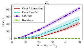
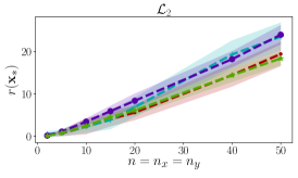
Figure 4. Scalability Experiments. The compared algorithms were run on $\mathcal{L}_{1}$ and $\mathcal{L}_{2}$ with $n_{x}=n_{y}\in\{2,5,10,15,20,40,50\}$ and $\text{\#FEs}=10^{4}\times n_{x}$. The markers indicate the average regret value surrounded by error bands signifying one standard deviation, obtained using $60$ independent runs. For Reckless, the CR variant is used with $s=0.5$.

Regret convergence of Reckless and the considered coevolutionary algorithms, given different #FEs, is shown in Figure 3. We re-iterate that the algorithms are re-run for each of the considered #FEs in a fixed-budget approach (Hansen et al., 2016), rather than setting the evaluation budget to its maximum and recording the regret at the #FEs of interest. With more #FEs, the regret of Reckless and MMDE consistently decrease. This is not the case for CoevA and CoevP due to their memoryless nature. In terms of problem dimensionality, MMDE scales poorly in comparison to the other algorithms as shown in Figure 4, whereas Reckless’s performance is consistent on $\mathcal{L}_{1}$ and comparable with that of CoevA on $\mathcal{L}_{2}$ outperforming both MMDE and CoevP.

Statistical Significance

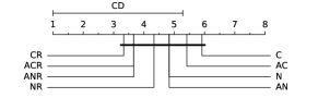
(b) Reckless variants

(c) Convergence

(d) Scalability

Figure 5. Critical Difference Plots. In our setup, a statistical significant difference was only found in (c) where Reckless outperforms CoevP. The Friedman test is used when comparing the performance of two or more algorithms as reported by differing evaluators. In our setup, the evaluators are the six benchmark problems—except for (d), where the evaluators are just $\mathcal{L}_{1}$ and $\mathcal{L}_{2}$. We run a Friedman test for each of our four experiments, with the null-hypothesis of same regret. In each of the four tests, the null-hypothesis was rejected with a p-value $<10^{-3}$, implying that at least one of the algorithms produced different regret values. In order to confirm which algorithm performed better, we carried out a post-hoc Nemenyi test. This test produces a critical difference (CD) score when provided with average ranks of the algorithms. The difference in average ranks between any two algorithms should be greater than this CD for one to conclude that one algorithm does better than the other.

We employ the non-parametric Friedman test, coupled with a post-hoc Nemenyi test with $\alpha=0.05$ (Demšar, 2006). The tests’ outcome is summarized in the CD plots shown in Figure 5. Overall, we infer that the experimental data is not sufficient to reach any conclusion regarding the differences in the algorithms’ performance. A statistically significant difference was only found between Reckless and CoevP in the regret convergence experiment (Figure 3). We hope that with more benchmark problems, statistical significance can be established, and we leave this for future work.

4.3. Application Example: Digital Filter Design

We apply Reckless and the other algorithms discussed in this work on an application presented by Charalambous (1979). The work introduces the problem of designing a digital filter such that its amplitude $|\mathcal{H}(x,\theta)|$ approximates a function $\mathcal{S(\psi)}$ = $|1-2\psi|$. $|\mathcal{H}(x,\theta)|$ is defined as:

$$A\prod\limits_{k=1}^{K}\Big{(}\frac{1+a_{k}^{2}+b_{k}^{2}+2b_{k}(2cos^{2}\theta-1)+2a_{k}(1+b_{k})cos\theta}{1+c_{k}^{2}+d_{k}^{2}+2d_{k}(2cos^{2}\theta-1)+2c_{k}(1+d_{k})cos\theta}\Big{)}^{\frac{1}{2}}$$

The authors then set this up as the following minimax problem:

$$\min\limits_{\mathbf{x}}\max\limits_{0\leq\psi\leq 1}|e(x,\psi)|,\text{where}\;e(x,\psi)=|\mathcal{H}(x,\theta)|-\mathcal{S(\psi)}$$

In this formulation, $\mathbf{x}=[A,a_{1},a_{2},\ldots,d_{1},d_{2}]$ ($K=2$ as chosen by the authors) to minimize and 1 variable ($\psi$) to maximize, i.e., $n_{x}=9$ and $n_{y}=1$ with $\mathcal{X}=[-1,1]^{n_{x}}$, $\mathcal{Y}=[0,1]^{n_{y}}$. We evaluate the four algorithms on this minimax problem. The performance of the algorithms is expressed in terms of regret. Lower the regret, higher the value of $\psi$ explored for a given minimum $x$. Table 1 records the regrets of the best points calculated by the four algorithms and the optimal point reported in (Charalambous, 1979). We evaluate each algorithm 60 times, for $10^{5}$ function evaluations, and report here median values. We see that Reckless outperforms all other algorithms in finding the best worst-case solution to the digital filter problem.

Table 1. Regret of the algorithms for the digital filter design.

(Charalambous, 1979)’s method	Reckless	MMDE	CoevA	CoevP
7.14$\times 10^{-3}$	4.16$\mathbf{\times 10^{-13}}$	5.09$\times 10^{-3}$	5.73$\times 10^{-6}$	4.36$\times 10^{-3}$

5. Conclusions

In this paper, we presented Reckless: a theoretically-founded framework tailored to black-box problems that are usually solved in a coevolutionary setup. Our proposition employed the stochastic gradient estimation of ES motivated by the experimental success of using gradients at approximate inner maximizers of minimax problems.

As demonstrated on scalable benchmark problems and a real-world application, Reckless outperforms the majority of the established coevolutionary algorithms, particularly on high-dimensional problems. Moreover, we found that minimax problems can be solved where outer minimization is given half of the inner maximization’s evaluation budget. Due to the limited number of evaluators (benchmark problems), statistical significance could not be established. In our future work, we hope that a larger set of benchmark problems can address this issue.

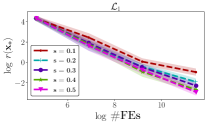
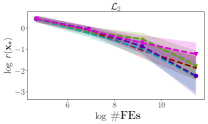
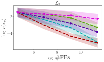
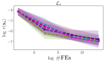
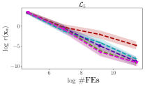
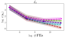
Figure 1. Reckless Steps along the Descent Direction. The markers indicate the average regret value surrounded by error bands signifying one standard deviation, obtained using $60$ independent runs of the variant N: NES without restart.

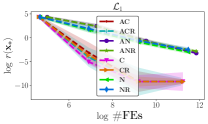
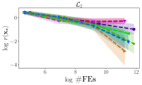
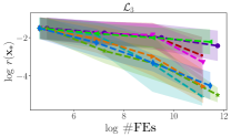
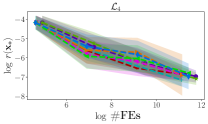
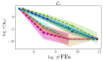
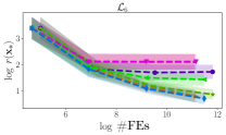
Figure 2. Reckless Variants. Each variant is denoted by a set of symbols as defined in Section 4. A: Antithetic, N: NES, C: CMA-ES, R: gradient-based restart. The markers indicate the average regret value surrounded by error bands signifying one standard deviation, obtained using $60$ independent runs.

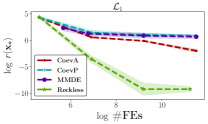
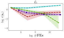
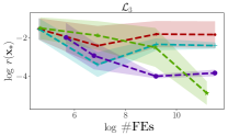
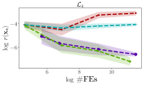
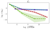
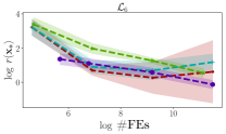
Figure 3. Regret Convergence of Minimax Algorithms. The markers indicate the average regret value surrounded by error bands signifying one standard deviation, obtained using $60$ independent runs. For Reckless, the CR variant is used with $s=0.5$.

Table 2. Description of benchmark problems. $\mathcal{L}_{1}$ and $\mathcal{L}_{2}$ were scaled with $n_{x},n_{y}\in\{2,5,10,15,20,40,50\}$ in scalability experiments.

$\mathcal{L}$	Definition	$\mathcal{X}$	$\mathcal{Y}$	$\mathbf{x}^{*}$	$\mathbf{y}^{*}$
$\mathcal{L}_{1}$	$\sum^{n}_{i=1}(x_{i}-5)^{2}-(y_{i}-5)^{2}$	$[0,10]^{3}$	$[0,10]^{3}$	$[5,5,5]$	$[5,5,5]$
$\mathcal{L}_{2}$	$\sum^{n}_{i=1}\min\{3-0.2x_{i}+0.3y_{i},3+0.2x_{i}-0.1y_{i}\}$	$[0,10]^{3}$	$[0,10]^{3}$	$[0,0,0]$	$[0,0,0]$
$\mathcal{L}_{3}$	$\frac{\sin(x-y)}{\sqrt{x^{2}+y^{2}}}$	$(0,10]$	$(0,10]$	$10$	$2.125683$
$\mathcal{L}_{4}$	$\frac{\cos\big{(}\sqrt{x^{2}+y^{2}}\big{)}}{\sqrt{x^{2}+y^{2}}+10}$	$[0,10]$	$[0,10]$	$7.044146$	$0$ or $10$
$\mathcal{L}_{5}$	$100(x_{2}-x^{2}_{1})^{2}+(1-x_{1})^{2}-y_{1}(x_{1}+x^{2}_{2})-y_{2}(x^{2}_{1}+x_{2})$	$[-0.5,0.5]\times[0,1]$	$[0,10]^{2}$	$[0.5,0.25]$	$[0,0]$
$\mathcal{L}_{6}$	$(x_{1}-2)^{2}+(x_{2}-1)^{2}+y_{1}(x^{2}_{1}-x_{2})+y_{2}(x_{1}+x_{2}-2)$	$[-1,3]^{2}$	$[0,10]^{2}$	$[1,1]$	any $\mathbf{y}\in\mathcal{Y}$

Table 3. Reckless setup given a budget allocation $s$ for steps along the descent direction and a finite number of function evaluations #FEs. In each of the $T$ iterations, the inner maximization and the outer minimization use $(1-s)v$ and $sv$ function evaluations, respectively.

$\bm{s}$	#FEs	$\bm{T}$	$\bm{(1-s)v}$	$\bm{sv}$	#FEs	$\bm{T}$	$\bm{(1-s)v}$	$\bm{sv}$
$0.1$	$10^{2}$	$1$	$90$	$10$	$10^{5}$	$41$	$2195$	$243$
$0.2$		$1$	$80$	$20$		$38$	$2105$	$526$
$0.3$		$1$	$70$	$30$		$36$	$1944$	$833$
$0.4$		$1$	$60$	$40$		$34$	$1764$	$1176$
$0.5$		$1$	$50$	$50$		$32$	$1562$	$1562$

(a) Reckless steps along the descent direction

References

- (1)
- Akimoto (2012) Youhei Akimoto. 2012. Analysis of a natural gradient algorithm on monotonic convex-quadratic-composite functions. In Proceedings of the 14th annual conference on Genetic and evolutionary computation. ACM, 1293–1300.
- Bäck et al. (2000) Thomas Bäck, David B Fogel, and Zbigniew Michalewicz. 2000. Evolutionary computation 1: Basic algorithms and operators. Vol. 1. CRC press.
- Brockhoff et al. (2010) Dimo Brockhoff, Anne Auger, Nikolaus Hansen, Dirk V Arnold, and Tim Hohm. 2010. Mirrored sampling and sequential selection for evolution strategies. In International Conference on Parallel Problem Solving from Nature. Springer, 11–21.
- Bubeck et al. (2012) Sébastien Bubeck, Nicolo Cesa-Bianchi, et al. 2012. Regret analysis of stochastic and nonstochastic multi-armed bandit problems. Foundations and Trends® in Machine Learning 5, 1 (2012), 1–122.
- Charalambous (1979) Christakis Charalambous. 1979. Acceleration of the leastpth algorithm for minimax optimization with engineering applications. Mathematical Programming 17, 1 (1979), 270–297.
- Conn et al. (2009) Andrew R Conn, Katya Scheinberg, and Luis N Vicente. 2009. Introduction to derivative-free optimization. Vol. 8. Siam.
- Cramer et al. (2009) Aaron M Cramer, Scott D Sudhoff, and Edwin L Zivi. 2009. Evolutionary algorithms for minimax problems in robust design. IEEE Transactions on Evolutionary Computation 13, 2 (2009), 444–453.
- Danskin (1966) John M Danskin. 1966. The theory of max-min, with applications. SIAM J. Appl. Math. 14, 4 (1966), 641–664.
- Demšar (2006) Janez Demšar. 2006. Statistical comparisons of classifiers over multiple data sets. Journal of Machine learning research 7, Jan (2006), 1–30.
- Glasmachers et al. (2010) Tobias Glasmachers et al. 2010. Exponential natural evolution strategies. In GECCO. ACM, 393–400.
- Hansen (2009) Nikolaus Hansen. 2009. Benchmarking a BI-population CMA-ES on the BBOB-2009 function testbed. In GECCO. ACM, 2389–2396.
- Hansen and Akimoto (2017) Nikolaus Hansen and Youhei Akimoto. 2017. Python implementation of CMA-ES. (2017). https://github.com/CMA-ES/pycma [Online; accessed 2018].
- Hansen and Ostermeier (2001) Nikolaus Hansen and Andreas Ostermeier. 2001. Completely derandomized self-adaptation in evolution strategies. Evolutionary computation 9, 2 (2001), 159–195.
- Hansen et al. (2016) Nikolaus Hansen et al. 2016. COCO: Performance assessment. arXiv:1605.03560 (2016).
- Herrmann (1999) Jeffrey W Herrmann. 1999. A genetic algorithm for minimax optimization problems. In CEC, Vol. 2. IEEE, 1099–1103.
- Huang et al. (2015) Ruitong Huang, Bing Xu, Dale Schuurmans, and Csaba Szepesvári. 2015. Learning with a strong adversary. arXiv:1511.03034 (2015).
- Huang et al. (2018) Alex Huang et al. 2018. Adversarial Deep Learning for Robust Detection of Binary Encoded Malware. arXiv:1801.02950 (2018).
- Jensen (2001) Mikkel T Jensen. 2001. Robust and flexible scheduling with evolutionary computation. Ph.D. Dissertation. University of Aarhus.
- Jensen (2003) Mikkel T Jensen. 2003. A new look at solving minimax problems with coevolutionary genetic algorithms. In Metaheuristics: computer decision-making. Springer, 369–384.
- Lehman et al. (2017) Joel Lehman, Jay Chen, Jeff Clune, and Kenneth O Stanley. 2017. ES Is More Than Just a Traditional Finite-Difference Approximator. arXiv:1712.06568 (2017).
- Loshchilov and Hutter (2016) Ilya Loshchilov and Frank Hutter. 2016. SGDR: stochastic gradient descent with restarts. arXiv:1608.03983 (2016).
- Loshchilov et al. (2012) Ilya Loshchilov, Marc Schoenauer, and Michele Sebag. 2012. Alternative restart strategies for CMA-ES. In International Conference on Parallel Problem Solving from Nature. Springer, 296–305.
- Madry et al. (2017) Aleksander Madry et al. 2017. Towards Deep Learning Models Resistant to Adversarial Attacks. In ICML 2017 Workshop.
- Morse et al. (2016) Gregory Morse et al. 2016. Simple Evolutionary Optimization Can Rival Stochastic Gradient Descent in Neural Networks. In GECCO. ACM, 477–484.
- Ollivier et al. (2017) Yann Ollivier, Ludovic Arnold, Anne Auger, and Nikolaus Hansen. 2017. Information-Geometric Optimization Algorithms: A Unifying Picture via Invariance Principles. Journal of Machine Learning Research 18, 18 (2017), 1–65. http://jmlr.org/papers/v18/14-467.html
- Powell (1973) Michael JD Powell. 1973. On search directions for minimization algorithms. Mathematical programming 4, 1 (1973), 193–201.
- Powell (1977) Michael James David Powell. 1977. Restart procedures for the conjugate gradient method. Mathematical programming 12, 1 (1977), 241–254.
- Qiu et al. (2017) Xin Qiu et al. 2017. A New Differential Evolution Algorithm for Minimax Optimization in Robust Design. IEEE Transactions on Cybernetics (2017).
- Salimans et al. (2017) Tim Salimans, Jonathan Ho, Xi Chen, and Ilya Sutskever. 2017. Evolution strategies as a scalable alternative to reinforcement learning. arXiv:1703.03864 (2017).
- Sharif et al. (2017) Mahmood Sharif et al. 2017. Adversarial Generative Nets: Neural Network Attacks on State-of-the-Art Face Recognition. arXiv:1801.00349 (2017).
- Valko et al. (2013) Michal Valko, Alexandra Carpentier, and Rémi Munos. 2013. Stochastic simultaneous optimistic optimization. In ICML. 19–27.
- Wierstra et al. (2014) Daan Wierstra et al. 2014. Natural evolution strategies. JMLR 15, 1 (2014), 949–980.
- Winkelbauer (2012) Andreas Winkelbauer. 2012. Moments and absolute moments of the normal distribution. arXiv:1209.4340 (2012).