Fluid heterogeneity detection based on the asymptotic distribution of the time-averaged mean squared displacement in single particle tracking experiments thanks: D.B.H. was partially supported by the awards DMS 1462992 (National Science Foundation), AI1 12029 and HL 108808 (National Institutes of Health), and Hill16XX0 (Cystic Fibrosis Foundation). G.D. was partially supported by the prime award no. W911NF-14-1-0475 from the Biomathematics subdivision of the Army Research Office, USA. The authors would like to thank John Fricks for his suggestions and comments on this paper. thanks: Keywords and phrases: mean squared displacement, asymptotic distribution, anomalous diffusion, fluid heterogeneity.

Kui Zhang1, Katelyn P. R. Crizer3, Mark H. Schoenfisch3, David B. Hill2 and Gustavo Didier1
1Department of Mathematics, Tulane University
2The Marsico Lung Institute and Department of Physics and Astronomy,
University of North Carolina at Chapel Hill
3Department of Chemistry, University of North Carolina at Chapel Hill
Abstract

A tracer particle is called anomalously diffusive if its mean squared displacement grows approximately as σ2tαsuperscript𝜎2superscript𝑡𝛼\sigma^{2}t^{\alpha} as a function of time t𝑡t for some constant σ2superscript𝜎2\sigma^{2}, where the diffusion exponent satisfies α1𝛼1\alpha\neq 1. In this article, we use recent results on the asymptotic distribution of the time-averaged mean squared displacement [20] to construct statistical tests for detecting physical heterogeneity in viscoelastic fluid samples starting from one or multiple observed anomalously diffusive paths. The methods are asymptotically valid for the range 0<α<3/20𝛼320<\alpha<3/2 and involve a mathematical characterization of time-averaged mean squared displacement bias and the effect of correlated disturbance errors. The assumptions on particle motion cover a broad family of fractional Gaussian processes, including fractional Brownian motion and many fractional instances of the generalized Langevin equation framework. We apply the proposed methods in experimental data from treated P. aeruginosa biofilms generated by the collaboration of the Hill and Schoenfisch Labs at UNC-Chapel Hill.

1 Introduction

In this paper, we start from the asymptotic distribution of the time-averaged mean squared displacement of nanometric tracer particles [20] to construct statistical protocols for detecting physical fluid heterogeneity. The assumptions on particle motion cover a broad family of fractional Gaussian processes, including fractional Brownian motion and many instances of the generalized Langevin equation framework. The testing protocols allowed providing more accurate quantitative analysis of experimental data from the Hill and Schoenfisch Labs (UNC-Chapel Hill), and the results reported in [73] were generally confirmed.

Improvements in light microscopy, fluorescence techniques, nanoparticle synthesis and high-speed video have ushered in a flurry of experimental activity [81]. Single particle tracking has become a common tool in many scientific areas, such as colloid physics [34], the microrheology of complex fluids [53, 83, 54, 45, 35] and the study of nanobiophysical systems, both in vivo and in vitro [2, 12]. This includes the diffusion of single molecules, e.g., proteins, on biopolymers such as DNA or microtubules, on surfaces or in lipid membranes, inside in vivo cells and in actin solutions [84, 26, 32, 89, 33, 61, 82, 95, 46, 67, 80, 4, 30], as well as two-dimensional biological membranes [58] and heterogeneuous tracer diffusion and first passage characteristics in two-dimensional crowded environments [23].

Of primary concern in the analysis of particle path data is the ensemble mean squared displacement (MSD), where X𝑋X is the tracer particle’s position. A basic dynamic characterization of the latter is given by the relation

X2(t)=𝔼X2(t)σ2tα,σ2,α>0,t0,𝝃:=(logσ2,α).formulae-sequencedelimited-⟨⟩superscript𝑋2𝑡𝔼superscript𝑋2𝑡proportional-tosuperscript𝜎2superscript𝑡𝛼superscript𝜎2𝛼0formulae-sequence𝑡0assign𝝃superscript𝜎2𝛼\langle X^{2}(t)\rangle={\mathbb{E}}X^{2}(t)\propto\sigma^{2}t^{\alpha},\quad\sigma^{2},\alpha>0,\quad t\geq 0,\quad{\boldsymbol{\xi}}:=(\log\sigma^{2},\alpha). (1)

In (1), α𝛼\alpha is the diffusion exponent and σ2=2Dsuperscript𝜎22𝐷\sigma^{2}=2D, where D𝐷D is the diffusivity constant. The parameter value α=1𝛼1\alpha=1 corresponds to classical diffusion. If α1𝛼1\alpha\neq 1, the stochastic process X𝑋X is said to be anomalously diffusive, more specifically sub- or superdiffusive depending on whether α<1𝛼1\alpha<1 or >1absent1>1, respectively. Anomalous diffusion may emerge, for example, as a consequence of binding-unbinding events, of geometrical constraints on the particle’s movement, or of fluid viscoelasticity [57, 77, 76, 49].

The dominant statistical technique in the biophysical literature for estimating the parameters σ2superscript𝜎2\sigma^{2} and α𝛼\alpha is based on the so-named time-averaged mean squared displacement (TAMSD). Suppose that a single particle experiment generates a tracer bead sample path with observations X(j)𝑋𝑗X(j), j=1,,N𝑗1𝑁j=1,\ldots,N. The pathwise statistic

MN(τ):=1Nτj=1Nτ{X(j+τ)X(j)}2assignsubscript𝑀𝑁𝜏1𝑁𝜏superscriptsubscript𝑗1𝑁𝜏superscript𝑋𝑗𝜏𝑋𝑗2M_{N}(\tau):=\frac{1}{N-\tau}\sum_{j=1}^{N-\tau}\{X(j+\tau)-X(j)\}^{2} (2)

is the TAMSD at lag value τ𝜏\tau, i.e., the statistical counterpart of the MSD X2(τ)delimited-⟨⟩superscript𝑋2𝜏\langle X^{2}(\tau)\rangle. One generates an estimator of 𝝃=(logσ2,α)𝝃superscript𝜎2𝛼{\boldsymbol{\xi}}=(\log\sigma^{2},\alpha) by means of the linear regression

logMN(τk)=logσ2+αlogτk+εk,k=1,,m,formulae-sequencesubscript𝑀𝑁subscript𝜏𝑘superscript𝜎2𝛼subscript𝜏𝑘subscript𝜀𝑘𝑘1𝑚\log M_{N}(\tau_{k})=\log\sigma^{2}+\alpha\log\tau_{k}+\varepsilon_{k},\quad k=1,\ldots,m, (3)

possibly over several independent particle paths, where m𝑚m is the number of lag values used and {εk}k=1,,msubscriptsubscript𝜀𝑘𝑘1𝑚\{\varepsilon_{k}\}_{k=1,\ldots,m} is a random vector with an unspecified distribution and correlated entries (see (7) and (22)). Plots of TAMSD curves as a function of the lag value τ𝜏\tau, often on a log-log scale, are widely reported as part of anomalous diffusion data analysis (e.g., [90, 50]). The choice of lag values τ1,,τmsubscript𝜏1subscript𝜏𝑚\tau_{1},\ldots,\tau_{m} reflects the analyst’s visual perception of the range where the slope of the TAMSD curves stabilize and thus indicate the true diffusive regime and power law.

The potential heterogeneity of fluid samples in fields such as microrheology implies that estimating 𝝃𝝃{\boldsymbol{\xi}} from single trajectories is of great interest [9, 11, 93, 51]. However, the experimental and statistical difficulties involved in estimating 𝝃𝝃{\boldsymbol{\xi}} based on the regression system (3) have been pointed out by many authors. A non-exhaustive list of issues includes limited fluorophore lifetimes, proteins diffusing out of the field of view, finite-resolution imaging and motion blurring due to camera integration times, measurement errors, the presence of drifts and intra-path correlation [71, 3, 60, 40, 93, 10, 56, 8, 36]. Such difficulties call for a deeper understanding of the stochastic behavior of the TAMSD and, accordingly, a wealth of literature on the subject has developed. Starting from an underlying fractional stochastic process, several properties of the TAMSD such as ergodicity were established [17, 59, 39, 13, 75, 6, 38]. In particular, finite sample exact characterizations and mathematically convenient approximations to the distribution of the TAMSD under Gaussianity are provided in [71, 27, 28, 6, 1, 65, 7, 29, 79, 22]. In [79], assuming an observed fractional Brownian motion (see Example 2.2), it is shown that the standard TAMSD-based estimator is consistent, with vanishing bias and variance.

We say that a cumulative distribution function (c.d.f.) F𝐹F gives the asymptotic distribution of a sequence of random variables {WN}Nsubscriptsubscript𝑊𝑁𝑁\{W_{N}\}_{N\in{\mathbb{N}}} if the c.d.f. FN(x)subscript𝐹𝑁𝑥F_{N}(x) of WNsubscript𝑊𝑁W_{N} converges to F(x)𝐹𝑥F(x) at every x𝑥x\in{\mathbb{R}} where F𝐹F is continuous. Results on convergence in distribution such as the classical central limit theorem (CLT; see Example 2.1) have a number of interesting statistical consequences. Typically, statements are robust, i.e., they hold for a multitude of models. Moreover, they naturally lead to useful data analysis protocols such as confidence intervals and hypothesis tests with error margins that are quantifiable and whose accuracy provably increases at an explicit rate (e.g., N𝑁\sqrt{N} for the CLT). In the probability literature, the study of the asymptotic distribution of sums of functions of Gaussian random variables has been carried out over many decades now (see [74, 85, 86, 21, 52, 24, 31, 25, 69] for just a few references). In the context of anomalous diffusion modeling, in turn, the related asymptotic distribution of the TAMSD was established in [20] for a broad class of Gaussian fractional stochastic processes. It was shown that the convergence in distribution of the TAMSD occurs at different rates, and that the limiting distribution may be Gaussian or non-Gaussian, all depending on the value of the diffusion exponent α𝛼\alpha. This made it possible, for example, to construct asymptotically valid confidence intervals for the anomalous diffusion parameters starting from a single observed particle path.

In this paper, we propose particle path-based statistical protocols for detecting fluid heterogeneity that builds upon the TAMSD’s asymptotic distribution. The protocols test fluid heterogeneity in two different experimental situations, namely,

  • (i)𝑖(i)

    assuming local physical homogeneity, whether different regions of the fluid are heterogeneous;

  • (ii)𝑖𝑖(ii)

    assuming global physical homogeneity of each fluid sample, whether two samples from each fluid are heterogeneous.

Hereinafter, these two senses are referred to as intra- and interfluid heterogeneity, respectively. The testing methodology is based on an improved single-path TAMSD-based estimation technique. To construct the latter, we tackle two of the main issues involved in TAMSD-based estimation, namely: (a) the presence of bias in log-TAMSD-based methods; and (b) the effect of correlated disturbances {εk}k=1,,msubscriptsubscript𝜀𝑘𝑘1𝑚\{\varepsilon_{k}\}_{k=1,\ldots,m} in (3). Starting from a concentration inequality [5], we address these issues by providing mathematical characterizations of the bias and finite sample estimation variance which are by themselves of interest, as well as by introducing procedures for bias-correction and nearly optimal estimation under intra-path correlation. Motivated by applications in viscoelastic diffusion, the single-path estimation and heterogeneity testing protocols are mathematically established for 0<α<3/20𝛼320<\alpha<3/2, which covers all the subdiffusive range and part of the superdiffusive regime, and are asymptotically valid. For the sake of completeness, we also discuss and provide computational studies on the strong superdiffusivity range 3/2α<232𝛼23/2\leq\alpha<2 (see Remark 3.2 on the difficulties involved in dealing with the possibly non-Gaussian asymptotic distribution of the TAMSD). To guide experimental practice under common technical constraints such as limited camera recording time, we also apply the proposed tools in investigating the difference between observing longer particle paths and using a larger number of particle paths of given length. To illustrate the use of the protocols in physical practice, we make inferences on fluid viscoelasticity with data from the Hill and Schoenfisch Labs (UNC-Chapel Hill) on biofilm eradication, as first reported and described in [73].

The paper is organized as follows. In Section 2, we summarize the key mathematical results on the asymptotic distribution of the TAMSD. In Section 3, assuming a single observed path of realistic length, we characterize the bias and the variance in TAMSD-based estimation to construct the improved single-path estimator and compare it with the standard TAMSD-based estimator in terms of statistical performance. In Section 4, assuming multiple observed paths, we use the estimator developed in Section 3 to construct statistical testing protocols for intra- and interfluid heterogeneity detection. In Section 5, we model and test fluid heterogeneity through experimental data. For the reader’s convenience, Section A of the Appendix contains mathematically accurate statements of the results in Section 2 and [20]. Sections B, C and D contain all new mathematical results and their proofs. Newly designed Matlab routines containing the estimation and testing protocols will be made available on the authors’ websites at the time of publication.

2 Background

Before we revisit the results in [20] on the asymptotic behavior of the TAMSD, for the sake of exposition we consider some classical results from probability theory.

Example 2.1.

Consider independent and identically distributed random variables X1,,XNsubscript𝑋1subscript𝑋𝑁X_{1},\ldots,X_{N}, each with mean X1=μdelimited-⟨⟩subscript𝑋1𝜇\langle X_{1}\rangle=\mu and finite variance VarX1:=X12X12=φ2>0assignVarsubscript𝑋1delimited-⟨⟩subscriptsuperscript𝑋21superscriptdelimited-⟨⟩subscript𝑋12superscript𝜑20{\mathrm{Var}}X_{1}:=\langle X^{2}_{1}\rangle-\langle X_{1}\rangle^{2}=\varphi^{2}>0. If X¯N=N1i=1NXisubscript¯𝑋𝑁superscript𝑁1subscriptsuperscript𝑁𝑖1subscript𝑋𝑖\overline{X}_{N}=N^{-1}\sum^{N}_{i=1}X_{i} denotes the sample mean, then the celebrated central limit theorem states that, for large N𝑁N, the distribution of the standardized sample mean approaches that of a standard normal, i.e.,

N(X¯Nμ)φd𝒩(0,1),N.formulae-sequencesuperscript𝑑𝑁subscript¯𝑋𝑁𝜇𝜑𝒩01𝑁\sqrt{N}\hskip 2.84526pt\frac{(\overline{X}_{N}-\mu)}{\varphi}\stackrel{{\scriptstyle d}}{{\rightarrow}}{\mathcal{N}}(0,1),\quad N\rightarrow\infty. (4)

Apart from naturally leading to confidence intervals and hypothesis tests, the convergence (4) also implies that X¯Nsubscript¯𝑋𝑁\overline{X}_{N} is a consistent estimator of μ𝜇\mu, namely, it converges in probability to μ𝜇\mu. This is so because

X¯Nμ=(φN)N(X¯Nμ)φP0,N.formulae-sequencesubscript¯𝑋𝑁𝜇𝜑𝑁𝑁subscript¯𝑋𝑁𝜇𝜑superscript𝑃0𝑁\overline{X}_{N}-\mu=\Big{(}\frac{\varphi}{\sqrt{N}}\Big{)}\sqrt{N}\hskip 2.84526pt\frac{(\overline{X}_{N}-\mu)}{\varphi}\stackrel{{\scriptstyle P}}{{\rightarrow}}0,\quad N\rightarrow\infty. (5)

The zero limit in probability in (5) stems from the fact that the vanishing term φ/N0𝜑𝑁0\varphi/\sqrt{N}\rightarrow 0 multiplies a standardized sample mean that converges in distribution (4) (see [78]).

Apart from distinct assumptions on the observations, the claims in [20] on the asymptotic behavior of the TAMSD are reminiscent of the classical statements (4) and (5), with two differences: (i)𝑖(i) the rate of convergence is not typically N𝑁\sqrt{N} in biophysical modeling; (ii)𝑖𝑖(ii) the asymptotic distribution of the TAMSD is not necessarily Gaussian.

So, consider the random vector

(MN(τ1),,MN(τm)),subscript𝑀𝑁subscript𝜏1subscript𝑀𝑁subscript𝜏𝑚\Big{(}M_{N}(\tau_{1}),\ldots,M_{N}(\tau_{m})\Big{)}, (6)

namely, a vector of TAMSD terms (2) at m𝑚m different lag values, obtained from one path of a Gaussian, stationary increment process. Fitting (3) and (6) by means of ordinary least squares (OLS) regression is the most intuitive way of constructing an estimator of the diffusion parameter vector 𝝃=(logσ2,α)𝝃superscript𝜎2𝛼{\boldsymbol{\xi}}=(\log\sigma^{2},\alpha). This corresponds to the common practice in the biophysical literature, both in experimental and methodological work (e.g., [90, 50, 11, 51] among many references). Throughout this paper,

𝑬stand=(Lstand,Astand)subscript𝑬standsubscript𝐿standsubscript𝐴stand{\boldsymbol{E}}_{{\mathrm{stand}}}=(L_{{\mathrm{stand}}},A_{{\mathrm{stand}}}) (7)

denotes this standard estimator (see (22) for a precise expression). In this framework, we need to make the lag sizes τ1,,τmsubscript𝜏1subscript𝜏𝑚\tau_{1},\ldots,\tau_{m} themselves go to infinity, though no faster than the sample size N𝑁N. This mathematically expresses the practical analysis of anomalous diffusion data: the lag size has to be

  • (1)1({\mathcal{L}}1)

    large enough for the TAMSD regime to become log-linear;

  • (2)2({\mathcal{L}}2)

    but, at the same time, not too large because of the increased variance of the TAMSD.

For a generic lag value τ𝜏\tau, we can model this idea by writing

τN.𝜏much-less-than𝑁\infty\leftarrow\tau\ll N. (8)

The limit and inequality in (8) express (1)1({\mathcal{L}}1) and (2)2({\mathcal{L}}2), respectively (the accurate mathematical statements are given by condition (53); see also Figure 1).

parameter range rate of convergence asymptotic distribution
0<α<3/20𝛼320<\alpha<3/2 Nτ1τα𝑁𝜏1superscript𝜏𝛼\sqrt{\frac{N}{\tau}}\frac{1}{\tau^{\alpha}} Gaussian
α=3/2𝛼32\alpha=3/2 NlogN1τ2𝑁𝑁1superscript𝜏2\sqrt{\frac{N}{\log N}}\frac{1}{\tau^{2}} Gaussian
3/2<α<232𝛼23/2<\alpha<2 N2ατ2superscript𝑁2𝛼superscript𝜏2\frac{N^{2-\alpha}}{\tau^{2}} non-Gaussian
Table 1: Asymptotic behavior of the TAMSD random vector (6) (see Theorem A.1).

parameter range rate of convergence joint asymptotic distribution consistency
Lstandsubscript𝐿standL_{{\mathrm{stand}}} Astandsubscript𝐴standA_{{\mathrm{stand}}}
0<α<3/20𝛼320<\alpha<3/2 Nτ1τα1logτ𝑁𝜏1superscript𝜏𝛼1𝜏\sqrt{\frac{N}{\tau}}\frac{1}{\tau^{\alpha}}\frac{1}{\log\tau} Nτ1τα𝑁𝜏1superscript𝜏𝛼\sqrt{\frac{N}{\tau}}\frac{1}{\tau^{\alpha}} Gaussian yes
α=3/2𝛼32\alpha=3/2 NlogN1τ21logτ𝑁𝑁1superscript𝜏21𝜏\sqrt{\frac{N}{\log N}}\frac{1}{\tau^{2}}\frac{1}{\log\tau} NlogN1τ2𝑁𝑁1superscript𝜏2\sqrt{\frac{N}{\log N}}\frac{1}{\tau^{2}} Gaussian yes
3/2<α<232𝛼23/2<\alpha<2 N2ατ21logτsuperscript𝑁2𝛼superscript𝜏21𝜏\frac{N^{2-\alpha}}{\tau^{2}}\frac{1}{\log\tau} N2ατ2superscript𝑁2𝛼superscript𝜏2\frac{N^{2-\alpha}}{\tau^{2}} non-Gaussian yes
Table 2: Asymptotic behavior of the standard TAMSD-based estimator (7) (see Corollary A.1).

The asymptotic distribution of the TAMSD random vector (6) after centering is briefly described in Table 1. This leads to the asymptotic behavior of the standard estimator (7), which is summarized in Table 2 in terms of convergence rate, asymptotic distribution and consistency. In both cases, the value of α𝛼\alpha determines the convergence rate and the nature of the asymptotic distribution. In particular, over almost the whole strong superdiffusivity range (i.e., over 3/2<α<232𝛼23/2<\alpha<2), the asymptotic distribution is non-Gaussian (Rosenblatt-type; see Theorem A.1 and [74, 85, 88, 91]). For any instance, by an argument analogous to (5), the standard estimator is consistent, i.e.,

𝑬standP𝝃.superscript𝑃subscript𝑬stand𝝃{\boldsymbol{E}}_{{\mathrm{stand}}}\stackrel{{\scriptstyle P}}{{\rightarrow}}\boldsymbol{\xi}. (9)

The family of stochastic processes for which the limits in distribution in Tables 1 and 2 hold is broad and contains a number of popular models. Three examples are fractional Brownian motion (fBm), fractional instances of the generalized Langevin equation (GLE) and the (integrated) fractional Ornstein-Uhlenbeck process (ifOU).

Example 2.2.

Together with the continuous time random walk, fBm is one of the most popular models of anomalous diffusion [87, 2]. For some value of the so-named Hurst parameter H(0,1)𝐻01H\in(0,1) and a variance parameter D>0𝐷0D>0, a fBm BH(t)subscript𝐵𝐻𝑡B_{H}(t) is the only Gaussian, stationary increment process with covariance function

BH(s)BH(t)=D{|t|2H+|s|2H|ts|2H},s,t.formulae-sequencedelimited-⟨⟩subscript𝐵𝐻𝑠subscript𝐵𝐻𝑡𝐷superscript𝑡2𝐻superscript𝑠2𝐻superscript𝑡𝑠2𝐻𝑠𝑡\langle B_{H}(s)B_{H}(t)\rangle=D\{|t|^{2H}+|s|^{2H}-|t-s|^{2H}\},\quad s,t\in{\mathbb{R}}. (10)

The particular parameter value H=1/2𝐻12H=1/2 corresponds to the ordinary Brownian motion (Wiener process). In view of (10), which implies exact self-similarity, for fBm the MSD scaling relation (1) holds as an equality, i.e.,

BH2(t)=σ2tα,t,formulae-sequencedelimited-⟨⟩subscriptsuperscript𝐵2𝐻𝑡superscript𝜎2superscript𝑡𝛼𝑡\langle B^{2}_{H}(t)\rangle=\sigma^{2}t^{\alpha},\quad t\in{\mathbb{R}}, (11)

where

σ2=2D,α=2H.formulae-sequencesuperscript𝜎22𝐷𝛼2𝐻\sigma^{2}=2D,\quad\alpha=2H. (12)
Example 2.3.

The GLE has been used as a universal model of anomalous diffusion in the biophysical field of microrheology [53, 96, 68, 66]. A subclass of interest of the GLE framework is the fractional GLE family [44, 43, 18], which is obtained almost surely as the solution of the stochastic differential equation

mdV(t)=λtΓ(ts)V(s)𝑑s𝑑t+dBH(t),1/2<H<1.formulae-sequence𝑚𝑑𝑉𝑡𝜆subscriptsuperscript𝑡Γ𝑡𝑠𝑉𝑠differential-d𝑠differential-d𝑡𝑑subscript𝐵𝐻𝑡12𝐻1m\hskip 2.84526ptdV(t)=-\lambda\int^{t}_{-\infty}\Gamma(t-s)V(s)dsdt+dB_{H}(t),\quad 1/2<H<1. (13)

In (13), m,λ>0𝑚𝜆0m,\lambda>0 and the memory kernel has the form Γ(t)=2H(2H1)|t|2H2Γ𝑡2𝐻2𝐻1superscript𝑡2𝐻2\Gamma(t)=2H(2H-1)|t|^{2H-2}, t0𝑡0t\neq 0, which is a consequence of invoking the fluctuation-dissipation relation [19, 51]. The integrated fractional generalized Langevin process (ifGL) is given by X(t)=0tV(s)𝑑s𝑋𝑡subscriptsuperscript𝑡0𝑉𝑠differential-d𝑠X(t)=\int^{t}_{0}V(s)ds, t>0𝑡0t>0, where {V(t)}t0subscript𝑉𝑡𝑡0\{V(t)\}_{t\geq 0} is a solution of the fractional GLE. For the ifGL, relation (1) holds with α=2(1H)𝛼21𝐻\alpha=2(1-H) (subdiffusive) as t𝑡t\rightarrow\infty.

Example 2.4.

The ifOU is given by X(t)=0tV(s)𝑑s𝑋𝑡subscriptsuperscript𝑡0𝑉𝑠differential-d𝑠X(t)=\int^{t}_{0}V(s)ds, t>0𝑡0t>0, where the so-named fractional Ornstein-Uhlenbeck process {V(t)}t0subscript𝑉𝑡𝑡0\{V(t)\}_{t\geq 0} is the almost surely continuous solution to the fBm-driven Langevin equation

dV(t)=λV(t)dt+φdBH(t),t0,λ>0,0<H<1formulae-sequence𝑑𝑉𝑡𝜆𝑉𝑡𝑑𝑡𝜑𝑑subscript𝐵𝐻𝑡formulae-sequence𝑡0formulae-sequence𝜆00𝐻1dV(t)=-\lambda V(t)dt+\varphi\hskip 1.42262ptdB_{H}(t),\quad t\geq 0,\quad\lambda>0,\quad 0<H<1 (14)

(see [14, 70]). The ifOU process is a mathematically convenient model of anomalous diffusion. In the subdiffusive range, it displays a similar correlation structure to that of the ifGL process. For the ifOU, relation (1) holds with (12) as t𝑡t\rightarrow\infty.

Remark 2.1.

The results in [20] do not cover some important anomalous diffusion models such as continuous time random walks. For the latter family of models, limit theorems typically involve distinct nonstandard asymptotic distributions depending on the assumptions (see, for instance, [55, 41] and references therein; for general guidelines on the use of the TAMSD, see [42]).

3 Improved TAMSD-based estimation

The standard estimator 𝑬stand=(Lstand,Astand)subscript𝑬standsubscript𝐿standsubscript𝐴stand{\boldsymbol{E}}_{{\mathrm{stand}}}=(L_{{\mathrm{stand}}},A_{{\mathrm{stand}}}) in (7) has at least two significant shortcomings: finite sample bias and suboptimal performance in the presence of correlation among the regression disturbance terms {εk}k=1,,Nsubscriptsubscript𝜀𝑘𝑘1𝑁\{\varepsilon_{k}\}_{k=1,\ldots,N}. We propose a single-path improved estimation protocol that addresses these issues. Accordingly, it involves two components, which we describe next. These two components involve asymptotically valid mathematical expressions for finite-sample bias and variance. Hereinafter, different lag values are expressed as

τk=wkτ,w1<<wk,formulae-sequencesubscript𝜏𝑘subscript𝑤𝑘𝜏subscript𝑤1subscript𝑤𝑘\tau_{k}=w_{k}\tau,\quad w_{1}<\ldots<w_{k}, (15)

for fixed constants wsubscript𝑤w_{\cdot}, where τ=τ(N)𝜏𝜏𝑁\tau=\tau(N) grows as function of N𝑁N.

(a) Bias correction. In TAMSD-based scaling analysis, there at least two sources of bias. First, bias appears if the particle movement is not exactly self-similar (not a fBm), i.e.,

X2(t)σ2tαover a range of t.delimited-⟨⟩superscript𝑋2𝑡superscript𝜎2superscript𝑡𝛼over a range of t\langle X^{2}(t)\rangle\neq\sigma^{2}t^{\alpha}\quad\textnormal{over a range of $t$}.

In fact, the deviation of the MSD from exact self-similarity or power scaling is generally controlled by the relation

|X2(t)σ2tα1|Ctδfor large t,delimited-⟨⟩superscript𝑋2𝑡superscript𝜎2superscript𝑡𝛼1𝐶superscript𝑡𝛿for large t\Big{|}\frac{\langle X^{2}(t)\rangle}{\sigma^{2}t^{\alpha}}-1\Big{|}\leq\frac{C}{t^{\delta}}\quad\textnormal{for large $t$}, (16)

for some constant σ2>0superscript𝜎20\sigma^{2}>0, where the deviation parameter δ>0𝛿0\delta>0 mostly depends on the high frequency behavior of the particle motion (see Proposition A.1). Second, even under self-similarity, bias stems from the elementary fact that the logarithm of the ensemble average and the ensemble average of the logarithm are distinct (e.g., [92, 63, 62, 64]). In the context of (3), this means that

logMN(τ)logMN(τ)=αlogτ+logσ2,τ.formulae-sequencedelimited-⟨⟩subscript𝑀𝑁𝜏subscript𝑀𝑁𝜏𝛼𝜏superscript𝜎2𝜏\langle\log M_{N}(\tau)\rangle\neq\log\langle M_{N}(\tau)\rangle=\alpha\log\tau+\log\sigma^{2},\quad\tau\in{\mathbb{N}}.

So, by reinterpreting logMN(τ)subscript𝑀𝑁𝜏\log M_{N}(\tau) itself as an estimator of αlogτ+logσ2𝛼𝜏superscript𝜎2\alpha\log\tau+\log\sigma^{2}, we can express the bias involved in TAMSD-based estimation as

logMN(τ)(αlogτ+logσ2)=τNβN(α,τ)+O(1τδ)+O(τN)delimited-⟨⟩subscript𝑀𝑁𝜏𝛼𝜏superscript𝜎2𝜏𝑁subscript𝛽𝑁𝛼𝜏𝑂1superscript𝜏𝛿𝑂𝜏𝑁\langle\log M_{N}(\tau)\rangle-(\alpha\log\tau+\log\sigma^{2})=-\frac{\tau}{N}\beta_{N}(\alpha,\tau)+O\Big{(}\frac{1}{\tau^{\delta}}\Big{)}+O\Big{(}\frac{\tau}{N}\Big{)} (17)

for the same δ>0𝛿0\delta>0 as in (16) (for 0<α<3/20𝛼320<\alpha<3/2 – see Theorem C.1; see also Remark 3.2 on the range 3/2α<232𝛼23/2\leq\alpha<2). The term of order O(τδ)𝑂superscript𝜏𝛿O(\tau^{-\delta}), then, is mostly determined by the high frequency behavior of the anomalously diffusive particle (see Figure 1 and expressions (52), (54)). In (17), the main bias factor is given by the function

βN(α,τ)=14τi=N+1N1(1|i|N){|iτ+1|α2|iτ|α+|iτ1|α}2.subscript𝛽𝑁𝛼𝜏14𝜏superscriptsubscript𝑖𝑁1𝑁11𝑖𝑁superscriptsuperscript𝑖𝜏1𝛼2superscript𝑖𝜏𝛼superscript𝑖𝜏1𝛼2\beta_{N}(\alpha,\tau)=\frac{1}{4\tau}\sum_{i=-N+1}^{N-1}\bigg{(}1-\frac{\left|i\right|}{N}\bigg{)}\Big{\{}\left|\frac{i}{\tau}+1\right|^{\alpha}-2\left|\frac{i}{\tau}\right|^{\alpha}+\left|\frac{i}{\tau}-1\right|^{\alpha}\Big{\}}^{2}. (18)

Note that (18) depends on the unknown parameter α𝛼\alpha. So, we use Astandsubscript𝐴standA_{{\mathrm{stand}}} and (18) to define an estimator of the bias vector by

(βN(Astand,τk))k=1,,m.subscriptsubscript𝛽𝑁subscript𝐴standsubscript𝜏𝑘𝑘1𝑚\Big{(}\beta_{N}(A_{{\mathrm{stand}}},\tau_{k})\Big{)}_{k=1,\ldots,m}. (19)

(b) Accounting for disturbance correlation. In linear estimation theory, the method for dealing with correlated random errors is called generalized least squares (GLS). In fact, the resulting GLS estimator is the best linear unbiased estimator, since it outperforms its OLS counterpart in terms of mean squared error (MSE) (see [15]).

In the context of TAMSD-based estimation, to better understand the difference between the standard, OLS-based estimator and the related GLS-based estimator, recast the vector system (3) as the regression model

𝐳=X𝝃+𝜺.𝐳𝑋𝝃𝜺{\mathbf{z}}=X\boldsymbol{\xi}+{\boldsymbol{\varepsilon}}. (20)

In (20), the term 𝝃𝝃\boldsymbol{\xi} is as in (1), and the dependent variable and the regressor are given by, respectively,

𝐳=(logMN(τk))k=1,,m,X=(1logτ11logτm).formulae-sequence𝐳subscriptsubscript𝑀𝑁subscript𝜏𝑘𝑘1𝑚𝑋1subscript𝜏11subscript𝜏𝑚{\mathbf{z}}=\Big{(}\log M_{N}(\tau_{k})\Big{)}_{k=1,\ldots,m},\quad X=\left(\begin{array}[]{cc}1&\log\tau_{1}\\ \vdots&\vdots\\ 1&\log\tau_{m}\\ \end{array}\right). (21)

It is well known that the expression

𝑬stand:=(XTX)1XT𝐳=(Lstand,Astand)Tassignsubscript𝑬standsuperscriptsuperscript𝑋𝑇𝑋1superscript𝑋𝑇𝐳superscriptsubscript𝐿standsubscript𝐴stand𝑇{\boldsymbol{E}}_{{\mathrm{stand}}}:=(X^{T}X)^{-1}X^{T}{\mathbf{z}}=(L_{{\mathrm{stand}}},\hskip 2.84526ptA_{{\mathrm{stand}}}\hskip 1.42262pt)^{T} (22)

gives the standard estimator (7) generated by the OLS solution to the system (20). By contrast, let

Υ(𝝃)=(υk1,k2(𝝃))k1,k2=1,,m,Υ𝝃subscriptsubscript𝜐subscript𝑘1subscript𝑘2𝝃formulae-sequencesubscript𝑘1subscript𝑘21𝑚\Upsilon({\boldsymbol{\xi}})=\Big{(}\upsilon_{k_{1},k_{2}}({\boldsymbol{\xi}})\Big{)}_{k_{1},k_{2}=1,\ldots,m}, (23)

be the finite sample covariance matrix of the vector 𝐳𝐳{\mathbf{z}} as in (21). The GLS solution is given by

(XTΥ(𝝃)1X)1XTΥ(𝝃)1𝐳,superscriptsuperscript𝑋𝑇Υsuperscript𝝃1𝑋1superscript𝑋𝑇Υsuperscript𝝃1𝐳(X^{T}\Upsilon({\boldsymbol{\xi}})^{-1}X)^{-1}X^{T}\Upsilon({\boldsymbol{\xi}})^{-1}{\mathbf{z}}, (24)

which involves the unknown matrix (23). In practice, then, one needs to estimate such matrix. For this purpose, we first establish the entrywise expansion

υk1,k2(𝝃)=τNςN(α,τk1,τk2)+O(τ1δN)+o(τN),k1,k2=1,,mformulae-sequencesubscript𝜐subscript𝑘1subscript𝑘2𝝃𝜏𝑁subscript𝜍𝑁𝛼subscript𝜏subscript𝑘1subscript𝜏subscript𝑘2𝑂superscript𝜏1𝛿𝑁𝑜𝜏𝑁subscript𝑘1subscript𝑘21𝑚\upsilon_{k_{1},k_{2}}({\boldsymbol{\xi}})=\frac{\tau}{N}\hskip 2.84526pt\varsigma_{N}(\alpha,\tau_{k_{1}},\tau_{k_{2}})+O\Big{(}\frac{\tau^{1-\delta}}{N}\Big{)}+o\Big{(}\frac{\tau}{N}\Big{)},\quad k_{1},k_{2}=1,\ldots,m (25)

(for 0<α<3/20𝛼320<\alpha<3/2 – see Theorem C.2; see also Remark 3.2 on the range 3/2α<232𝛼23/2\leq\alpha<2). In (25), the main variance factor is given by

ςN(α,τk1,τk2)=12τi=N+1N1(1|i|N){|iτk1τk2+τk1τk2|α|iτk1τk2+τk1τk2τk2τk1|α\varsigma_{N}(\alpha,\tau_{k_{1}},\tau_{k_{2}})=\frac{1}{2\tau}\sum_{i=-N+1}^{N-1}\bigg{(}1-\frac{\left|i\right|}{N}\bigg{)}\bigg{\{}\left|\frac{i}{\sqrt{\tau_{k_{1}}\tau_{k_{2}}}}+\sqrt{\frac{\tau_{k_{1}}}{\tau_{k_{2}}}}\right|^{\alpha}-\left|\frac{i}{\sqrt{\tau_{k_{1}}\tau_{k_{2}}}}+\sqrt{\frac{\tau_{k_{1}}}{\tau_{k_{2}}}}-\sqrt{\frac{\tau_{k_{2}}}{\tau_{k_{1}}}}\right|^{\alpha}
|iτk1τk2|α+|iτk1τk2τk2τk1|α}2.-\left|\frac{i}{\sqrt{\tau_{k_{1}}\tau_{k_{2}}}}\right|^{\alpha}+\left|\frac{i}{\sqrt{\tau_{k_{1}}\tau_{k_{2}}}}-\sqrt{\frac{\tau_{k_{2}}}{\tau_{k_{1}}}}\right|^{\alpha}\bigg{\}}^{2}. (26)

Note that expression (26) does not involve the constant σ2superscript𝜎2\sigma^{2}, but it is still a function of the unknown parameter α𝛼\alpha. Second, and in view of this, we can use Astandsubscript𝐴standA_{{\mathrm{stand}}} and (26) to define an estimator of the covariance matrix by

Υ(Astand):=(τNςN(Astand,τk1,τk2))k1,k2=1,,m.assignΥsubscript𝐴standsubscript𝜏𝑁subscript𝜍𝑁subscript𝐴standsubscript𝜏subscript𝑘1subscript𝜏subscript𝑘2formulae-sequencesubscript𝑘1subscript𝑘21𝑚\Upsilon(A_{{\mathrm{stand}}}):=\Big{(}\frac{\tau}{N}\varsigma_{N}(A_{{\mathrm{stand}}},\tau_{k_{1}},\tau_{k_{2}})\Big{)}_{k_{1},k_{2}=1,\ldots,m}.\vspace{1mm} (27)

Drawing upon (a) and (b), we can further construct an improved estimator of 𝝃𝝃{\boldsymbol{\xi}} by a quasi-GLS procedure based on the estimator Υ(Astand)Υsubscript𝐴stand\Upsilon(A_{{\mathrm{stand}}}) and by replacing (3) with the bias-corrected regression system

logMN(τk)+τkNβN(Astand,τk)=logσ2+αlogτk+εk,k=1,,m.formulae-sequencesubscript𝑀𝑁subscript𝜏𝑘subscript𝜏𝑘𝑁subscript𝛽𝑁subscript𝐴standsubscript𝜏𝑘superscript𝜎2𝛼subscript𝜏𝑘subscript𝜀𝑘𝑘1𝑚\log M_{N}(\tau_{k})+\frac{\tau_{k}}{N}\beta_{N}(A_{{\mathrm{stand}}},\tau_{k})=\log\sigma^{2}+\alpha\log\tau_{k}+\varepsilon_{k},\quad k=1,\ldots,m. (28)

The resulting estimator can be expressed as

𝑬=(L,A)=(XTΥ1(Astand)X)1XTΥ1(Astand)𝐲,𝑬𝐿𝐴superscriptsuperscript𝑋𝑇superscriptΥ1subscript𝐴stand𝑋1superscript𝑋𝑇superscriptΥ1subscript𝐴stand𝐲{\boldsymbol{E}}=(L,A)=(X^{T}\Upsilon^{-1}(A_{{\mathrm{stand}}})X)^{-1}X^{T}\Upsilon^{-1}(A_{{\mathrm{stand}}}){\mathbf{y}}, (29)

where X𝑋X is again as in (21) and

𝐲=(logMN(τ1)+τ1NβN(Astand,τ1)logMN(τm)+τmNβN(Astand,τm)).𝐲subscript𝑀𝑁subscript𝜏1subscript𝜏1𝑁subscript𝛽𝑁subscript𝐴standsubscript𝜏1subscript𝑀𝑁subscript𝜏𝑚subscript𝜏𝑚𝑁subscript𝛽𝑁subscript𝐴standsubscript𝜏𝑚{\mathbf{y}}=\left(\begin{array}[]{c}\log M_{N}(\tau_{1})+\frac{\tau_{1}}{N}\beta_{N}(A_{{\mathrm{stand}}},\tau_{1})\\ \vdots\\ \log M_{N}(\tau_{m})+\frac{\tau_{m}}{N}\beta_{N}(A_{{\mathrm{stand}}},\tau_{m})\\ \end{array}\right). (30)

For the reader’s convenience, the construction of the estimator 𝑬𝑬{\boldsymbol{E}} is summarized in the form of pseudocode in Appendix D.

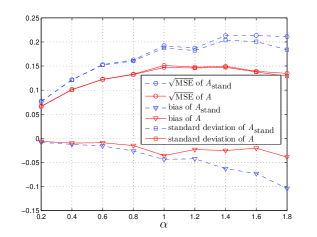
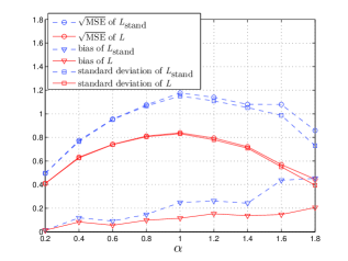
To compare the performances of 𝑬𝑬{\boldsymbol{E}} and 𝑬standsubscript𝑬stand{\boldsymbol{E}}_{{\mathrm{stand}}}, we generated 1000 independent paths of length 210superscript2102^{10} and estimated the diffusion exponent based on the two methods. Figure 2 displays the results in terms of Monte Carlo bias, standard deviation and square root MSE. The improved estimator 𝑬𝑬{\boldsymbol{E}} outperforms the usual estimator 𝑬standsubscript𝑬stand{\boldsymbol{E}}_{{\mathrm{stand}}} by any of the three criteria for different values of α𝛼\alpha.

Remark 3.1.

Note that the main bias and variance factors βN(α,τ)subscript𝛽𝑁𝛼𝜏\beta_{N}(\alpha,\tau) and ςN(α,τk1,τk2)subscript𝜍𝑁𝛼subscript𝜏subscript𝑘1subscript𝜏subscript𝑘2\varsigma_{N}(\alpha,\tau_{k_{1}},\tau_{k_{2}}) in (18) and (26), respectively, converge as N𝑁N\rightarrow\infty (see Lemma C.1). Moreover, after standardization, the estimator (29) is provably asymptotically normal and consistent for 0<α<3/20𝛼320<\alpha<3/2 (see (35) in Section 4 and Proposition C.1). See also Remark 3.2 on the range 3/2α<232𝛼23/2\leq\alpha<2.

Remark 3.2.

Although we do not provide proofs in this paper, the methods developed in this section and also in Section 4 can be extended to the strongly superdiffusive range 3/2α<232𝛼23/2\leq\alpha<2. For example, due to nonstandard convergence rates, expressions (17) and (25) hold after replacing O(τN)𝑂𝜏𝑁O(\frac{\tau}{N}) with O((τlogNN))𝑂𝜏𝑁𝑁O((\frac{\tau\log N}{N})) (for α=3/2𝛼32\alpha=3/2) or O((τN)42α)𝑂superscript𝜏𝑁42𝛼O((\frac{\tau}{N})^{4-2\alpha}) (for 3/2<α<232𝛼23/2<\alpha<2). Likewise, the asymptotic non-Gaussian distribution of the estimator (35) in Section 4, with nonstandard convergence rates, can be established. However, inference involving the nonstandard limiting distribution can be cumbersome, and the computational studies in this section and in Section 4 show that the methods in the proposed format work reasonably well for realistic path lengths. See also [20], Remark 2, on how to construct asymptotically valid confidence intervals for 𝝃𝝃{\boldsymbol{\xi}} based on the standard estimator 𝑬standsubscript𝑬stand{\boldsymbol{E}}_{{\mathrm{stand}}} assuming prior knowledge that 3/2<α<232𝛼23/2<\alpha<2.

Refer to caption
Refer to caption
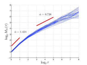
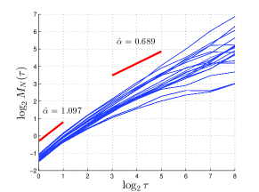
Figure 1: Bias and inconsistency over small scales τ𝜏\tau vs vanishing bias and consistency as τ𝜏\tau\rightarrow\infty. In general, taking the double limit τ,N𝜏𝑁\tau,N\rightarrow\infty (see (8)) is necessary. Over fixed (“small”) lag values τ𝜏\tau, TAMSD-based estimation is biased and, for most anomalous diffusion models other than fBm, inconsistent. As mathematically characterized by expansion (17), estimation bias is fundamentally a consequence of the fact that loglog\langle\log\cdot\rangle\neq\log\langle\cdot\rangle and of the presence of the small scale factor O(τδ)𝑂superscript𝜏𝛿O(\tau^{-\delta}), whereas, in turn, inconsistency generally appears as a consequence of this same factor. The left and right plots show, respectively, 20 independent ifOU paths (length 211superscript2112^{11}, α=0.6𝛼0.6\alpha=0.6) and 20 particle paths (length 1800) from P. aeruginosa biofilm after COS2-NO treatment at concentration level 8 mg ml-1. The first and second red lines in each plot indicate, respectively, the fitted slope over small (τ=1,2𝜏12\tau=1,2) and large (τ=8,32𝜏832\tau=8,32) lag values. Based on the former lag values, A=1.42𝐴1.42A=1.42 and 1.10 (evidence of superdiffusivity) for simulated and experimental data, respectively, whereas, by contrast, A=0.70𝐴0.70A=0.70 and 0.69 (evidence of subdiffusivity) based on the latter. This illustrates the fact that bias and inconsistency vanish when τ𝜏\tau (and N𝑁N) becomes large.
Refer to caption
Refer to caption
Figure 2: Comparative analysis of bias, standard deviation and MSE of the estimators 𝑬𝑬{\boldsymbol{E}} (see (29)) and 𝑬standsubscript𝑬stand{\boldsymbol{E}}_{{\mathrm{stand}}} (see (7)) as a function of diffusion exponents α𝛼\alpha (x𝑥x-axis). Left plot: estimation of α𝛼\alpha. Right plot: estimation of logσ2superscript𝜎2\log\sigma^{2}. Solid and dashed lines represent 𝑬𝑬{\boldsymbol{E}} and 𝑬standsubscript𝑬stand{\boldsymbol{E}}_{{\mathrm{stand}}}, respectively. For any parameter value α𝛼\alpha, the proposed estimator 𝑬𝑬{\boldsymbol{E}} has smaller bias, standard deviation and square root MSE than 𝑬standsubscript𝑬stand{\boldsymbol{E}}_{{\mathrm{stand}}}. The total number of Monte Carlo runs is 1000 based on paths of length 210superscript2102^{10}.

4 Testing heterogeneity

Single particle tracking experiments with viscoelastic diffusion often generate data in the form of multiple particle paths. As discussed in the Introduction, fluid heterogeneity can be tested in the intra- and interfluid senses. The pathwise framework constructed in Section 3 can be used in new testing protocols with good finite sample and asymptotic properties. We remind the reader that the mathematical statements cover the diffusion exponent range 0<α<3/20𝛼320<\alpha<3/2 (subdiffusive and mildly superdiffusive range), though we also include computational experiments for the strongly superdiffusive range 3/2α<232𝛼23/2\leq\alpha<2.

Tables 3 and 4 display the proposed framework. For each type of fluid heterogeneity, they show the appropriate hypotheses and testing procedures, respectively. In the remainder of this section, we provide a detailed description of the protocols. To set the notation, we recall that, for a given a hypothesis test, the conditional probability

(H0 is rejected |𝝃 satisfies H0)=:ϵ[0,1]{\mathbb{P}}(H_{0}\textnormal{ is rejected }|\hskip 1.42262pt{\boldsymbol{\xi}}\textnormal{ satisfies }H_{0})=:\epsilon\in[0,1] (31)

is called the size (or significance level) of the test, whereas the function

𝝃(H0 is rejected |𝝃 satisfies H1)[0,1]maps-to𝝃conditionalsubscript𝐻0 is rejected 𝝃 satisfies subscript𝐻101{\boldsymbol{\xi}}\mapsto{\mathbb{P}}(H_{0}\textnormal{ is rejected }|\hskip 1.42262pt{\boldsymbol{\xi}}\textnormal{ satisfies }H_{1})\in[0,1] (32)

is called the power of the test.

heterogeneity H0subscript𝐻0H_{0} Hasubscript𝐻𝑎H_{a}
intrafluid 𝝃1==𝝃νsubscript𝝃1subscript𝝃𝜈{\boldsymbol{\xi}}_{1}=\cdots={\boldsymbol{\xi}}_{\nu} 𝝃i𝝃jsubscript𝝃𝑖subscript𝝃𝑗\hskip 8.53581pt{\boldsymbol{\xi}}_{i}\neq{\boldsymbol{\xi}}_{j} for some 1i,jνformulae-sequence1𝑖𝑗𝜈1\leq i,j\leq\nu
interfluid 𝝃I=𝝃IIsubscript𝝃Isubscript𝝃II{\boldsymbol{\xi}}_{\mathrm{I}}={\boldsymbol{\xi}}_{\mathrm{II}} 𝝃I𝝃IIsubscript𝝃Isubscript𝝃II{\boldsymbol{\xi}}_{\mathrm{I}}\neq{\boldsymbol{\xi}}_{\mathrm{II}}
Table 3: Hypotheses

heterogeneity rejection region test statistic number of paths
intrafluid Rintra (see (38))subscript𝑅intra (see (38))R_{\textnormal{intra}}\textnormal{ (see \eqref{e:R-intra})} S12,S22 (see (37))subscriptsuperscript𝑆21subscriptsuperscript𝑆22 (see (37))S^{2}_{1},S^{2}_{2}\textnormal{ (see \eqref{e:S-xihat})} ν𝜈\nu
interfluid Rinter (see (46))subscript𝑅inter (see (46))R_{\textnormal{inter}}\textnormal{ (see \eqref{e:R-inter})} T1,T2 (see (45))subscript𝑇1subscript𝑇2 (see (45))T_{1},T_{2}\textnormal{ (see \eqref{e:two_fluid_ts})} νIsubscript𝜈I\nu_{\mathrm{I}}, νIIsubscript𝜈II\nu_{\mathrm{II}}
Table 4: Tests

Intrafluid heterogeneity. Suppose ν𝜈\nu\in{\mathbb{N}} bead diffusion paths of length N𝑁N from a single fluid sample are available. If the fluid is physically homogeneous, it is expected to generate particle paths with nearly identical parameter values 𝝃𝝃{\boldsymbol{\xi}}. The alternative is that 𝝃i𝝃jsubscript𝝃𝑖subscript𝝃𝑗{\boldsymbol{\xi}}_{i}\neq{\boldsymbol{\xi}}_{j} for some pair i,j𝑖𝑗i,j, namely, their anomalous diffusion parameters differ. These two possibilities, labeled H0subscript𝐻0H_{0} and Hasubscript𝐻𝑎H_{a}, respectively, are listed on the row “intrafluid” in Table 3.

Starting from the ν𝜈\nu particle paths, let

𝑬i,i=1,,ν,formulae-sequencesubscript𝑬𝑖𝑖1𝜈{\boldsymbol{E}}_{i},\quad i=1,\ldots,\nu, (33)

be vector-valued estimators as in (29). For the purpose of constructing a test statistic, we need a normalized (standardized) estimator. Note that the variance of the GLS-type solution (24) is given by

(XTΥ1(𝝃)X)1superscriptsuperscript𝑋𝑇superscriptΥ1𝝃𝑋1(X^{T}\Upsilon^{-1}({\boldsymbol{\xi}})X)^{-1} (34)

(cf. [15]). So, define a standardized estimator by

𝒁i=(Zi,1Zi,2)=Λ1/2(Astand,i)𝑬i,i=1,,ν,formulae-sequencesubscript𝒁𝑖subscript𝑍𝑖1subscript𝑍𝑖2superscriptΛ12subscript𝐴stand𝑖subscript𝑬𝑖𝑖1𝜈{\boldsymbol{Z}}_{i}=\left(\begin{array}[]{c}Z_{i,1}\\ Z_{i,2}\\ \end{array}\right)=\Lambda^{-1/2}(A_{{\mathrm{stand}},i}){\boldsymbol{E}}_{i},\quad i=1,\ldots,\nu, (35)

where

Λ(Astand,i):=(XTΥ1(Astand,i)X)1assignΛsubscript𝐴stand𝑖superscriptsuperscript𝑋𝑇superscriptΥ1subscript𝐴stand𝑖𝑋1\Lambda(A_{{\mathrm{stand}},i}):=(X^{T}\Upsilon^{-1}(A_{{\mathrm{stand}},i})X)^{-1} (36)

and the variance estimator Υ(Astand,i)Υsubscript𝐴stand𝑖\Upsilon(A_{{\mathrm{stand}},i}) is given by (27). Then, (35) converges in distribution to ν𝜈\nu independent and identically distributed normal random vectors with uncorrelated entries (see Proposition C.1). So, for Z¯j=ν1i=1νZi,jsubscript¯𝑍𝑗superscript𝜈1superscriptsubscript𝑖1𝜈subscript𝑍𝑖𝑗\overline{Z}_{j}=\nu^{-1}\sum_{i=1}^{\nu}Z_{i,j}, let

Sj2=1ν1i=1ν(Zi,jZ¯j)2,j=1,2,formulae-sequencesubscriptsuperscript𝑆2𝑗1𝜈1superscriptsubscript𝑖1𝜈superscriptsubscript𝑍𝑖𝑗subscript¯𝑍𝑗2𝑗12S^{2}_{j}=\frac{1}{\nu-1}\sum_{i=1}^{\nu}(Z_{i,j}-\overline{Z}_{j})^{2},\quad j=1,2, (37)

be the normalized and decorrelated sample variances of {Zi,j}i=1,,νsubscriptsubscript𝑍𝑖𝑗𝑖1𝜈\{Z_{i,j}\}_{i=1,\ldots,\nu}, j=1,2𝑗12j=1,2, as in (35). Then, under H0subscript𝐻0H_{0},

((ν1)S12,(ν1)S22)d(𝒳1,𝒳2),𝒳jχν12,j=1,2,formulae-sequencesuperscript𝑑𝜈1subscriptsuperscript𝑆21𝜈1subscriptsuperscript𝑆22subscript𝒳1subscript𝒳2formulae-sequencesimilar-tosubscript𝒳𝑗subscriptsuperscript𝜒2𝜈1𝑗12\Big{(}(\nu-1)S^{2}_{1},(\nu-1)S^{2}_{2}\Big{)}\stackrel{{\scriptstyle d}}{{\rightarrow}}({\mathcal{X}}_{1},{\mathcal{X}}_{2}),\quad{\mathcal{X}}_{j}\sim\chi^{2}_{\nu-1},\quad j=1,2,

as N𝑁N\rightarrow\infty, where 𝒳1subscript𝒳1{\mathcal{X}}_{1} and 𝒳2subscript𝒳2{\mathcal{X}}_{2} are independent random variables. To test heterogeneity at significance level ϵitalic-ϵ\epsilon, we can use Bonferroni-type correction (e.g., [15], section 5.3) and reject the null hypothesis H0subscript𝐻0H_{0} if

Rintra:(ν1)S12>χν1,ϵ/22or(ν1)S22>χν1,ϵ/22,:subscript𝑅intraformulae-sequence𝜈1subscriptsuperscript𝑆21subscriptsuperscript𝜒2𝜈1italic-ϵ2or𝜈1subscriptsuperscript𝑆22subscriptsuperscript𝜒2𝜈1italic-ϵ2R_{\textnormal{intra}}:(\nu-1)S^{2}_{1}>\chi^{2}_{\nu-1,\epsilon/2}\quad\textnormal{or}\quad(\nu-1)S^{2}_{2}>\chi^{2}_{\nu-1,\epsilon/2}, (38)

where χν1,ϵ/22subscriptsuperscript𝜒2𝜈1italic-ϵ2\chi^{2}_{\nu-1,\epsilon/2} is a chi-square quantile (c.f. Table 4, “intrafluid” rows).

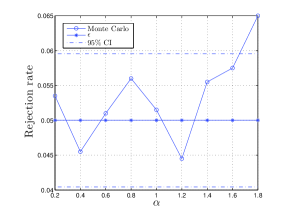
To check the size of the test (38) over finite samples, we conducted a Monte Carlo study with 50 simulated paths of length 212superscript2122^{12} and recorded whether or not the null hypothesis H0subscript𝐻0H_{0} is rejected at ϵ=0.05italic-ϵ0.05\epsilon=0.05 significance level. This procedure was repeated 2000 times. Since each outcome is a Bernoulli trial (reject or not H0subscript𝐻0H_{0}), the simulation rejection rate follows a binomial distribution with n=2000𝑛2000n=2000 and p=0.05𝑝0.05p=0.05. Thus, a normal approximation to the 95% confidence interval of the rejection rate gives (0.040,0.060)0.0400.060(0.040,0.060). As shown in Figure 3, left plot, the observed simulation rejection rate was around 0.05 and within the 95% confidence interval (for 0<α<3/20𝛼320<\alpha<3/2), as expected. Unreported computational experiments for different significance levels lead to analogous conclusions.

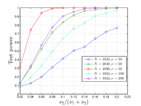
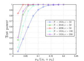
Figure 4 displays Monte Carlo power curves for the intrafluid test. The study was conducted with a total of ν=ν1+ν2𝜈subscript𝜈1subscript𝜈2\nu=\nu_{1}+\nu_{2} paths, where ν1subscript𝜈1\nu_{1} and ν2subscript𝜈2\nu_{2} have diffusion exponents α1=1subscript𝛼11\alpha_{1}=1 and α2subscript𝛼2\alpha_{2}, respectively, and α2=0.8subscript𝛼20.8\alpha_{2}=0.8 (left plot) or α2=0.7subscript𝛼20.7\alpha_{2}=0.7 (right plot). In each plot, the x𝑥x-axis represents the proportion of paths

ν2ν1+ν2subscript𝜈2subscript𝜈1subscript𝜈2\frac{\nu_{2}}{\nu_{1}+\nu_{2}} (39)

with diffusion exponent α=α2𝛼subscript𝛼2\alpha=\alpha_{2}. The power curves quickly converge to 1 as a function of the ratio (39), especially for the more distinguishable value α2=0.7<1=α1subscript𝛼20.71subscript𝛼1\alpha_{2}=0.7<1=\alpha_{1}.

When α>3/2𝛼32\alpha>3/2, under H0subscript𝐻0H_{0} the estimators (33) converge in distribution to ν𝜈\nu independent and identically distributed non-Gaussian random vectors. Hence, so do the estimators (35). In this case, the marginal distributions of the decorrelated vector ((ν1)S12,(ν1)S22)𝜈1subscriptsuperscript𝑆21𝜈1subscriptsuperscript𝑆22((\nu-1)S^{2}_{1},(\nu-1)S^{2}_{2}) do not approach chi-squared distributions. In computational experiments, the size of the intrafluid test (38) did not significantly deviate from the 0.05 target for α=1.6𝛼1.6\alpha=1.6, indicating that the nonstandard asymptotic behavior is not a concern for paths of length 212superscript2122^{12}. Deviation was significant for the extreme value α=1.8𝛼1.8\alpha=1.8, suggesting that approximating the test size by simulation may be generally recommendable for greater accuracy (see Figure 3, left plot).
Refer to caption
Refer to caption
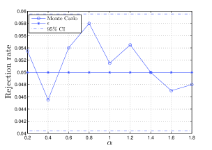
Figure 3: Intra- and interfluid heterogeneity: test sizes. Monte Carlo sizes of the intrafluid test (left plot; see (38)) and interfluid test (right plot; see (46)) as a function of the diffusion exponent α𝛼\alpha (x𝑥x-axis). For every value of α𝛼\alpha, each of 2000 Monte Carlo runs consisted of generating 50 independent paths of length 212superscript2122^{12} and conducting a test at ϵ=0.05italic-ϵ0.05\epsilon=0.05 (see (31)) or, equivalently, 95% confidence level. The Monte Carlo rejection rate is very close to the theoretical value of ϵ=0.05italic-ϵ0.05\epsilon=0.05 for almost all values of α𝛼\alpha.
Refer to caption
Refer to caption
Figure 4: Intrafluid heterogeneity: test power. Simulations were conducted with a total of ν=ν1+ν2𝜈subscript𝜈1subscript𝜈2\nu=\nu_{1}+\nu_{2} paths, where ν1subscript𝜈1\nu_{1} and ν2subscript𝜈2\nu_{2} of them displayed diffusion exponents α=α1=1𝛼subscript𝛼11\alpha=\alpha_{1}=1 and α=α2𝛼subscript𝛼2\alpha=\alpha_{2}, respectively. In each plot, the y𝑦y-axis represents the observed test power, or rejection rates (see (32)), and the x𝑥x-axis is the proportion of paths with α=α2𝛼subscript𝛼2\alpha=\alpha_{2} (see (39)), starting at 0.02. The total number of Monte Carlo runs is 2000. Left plot: α2=0.8subscript𝛼20.8\alpha_{2}=0.8. Right plot: α2=0.7subscript𝛼20.7\alpha_{2}=0.7.

Interfluid heterogeneity. Now suppose νIsubscript𝜈I\nu_{\mathrm{I}} and νIIsubscript𝜈II\nu_{\mathrm{II}} paths,

νI,νII,subscript𝜈Isubscript𝜈II\nu_{\mathrm{I}},\nu_{\mathrm{II}}\in{\mathbb{N}}, (40)

are obtained from two physically homogeneous fluid samples I and II, respectively. We are interested in testing whether the samples I and II are homogeneous, namely, whether or not particle diffusion in the fluid samples displays the same underlying parameter value 𝝃𝝃\boldsymbol{\xi}. These two possibilities, labeled H0subscript𝐻0H_{0} and Hasubscript𝐻𝑎H_{a}, respectively, are described on the row “interfluid” in Table 3.

Since multiple (independent) particle paths are assumed available for each fluid sample, we can construct an estimator involving all available TAMSD terms. In fact, first define the overall average mean squared displacement over ν𝜈\nu TAMSD terms (AMSD) by

MN(τ)=1ν=1νMN(τ).subscriptsuperscript𝑀𝑁𝜏1𝜈subscriptsuperscript𝜈1subscript𝑀𝑁subscript𝜏M^{*}_{N}(\tau)=\frac{1}{\nu}\sum^{\nu}_{\ell=1}M_{N}(\tau)_{\ell}. (41)

By independence,

MN(τ)=MN(τ)=X2(τ),VarMN(τ)=1νVarMN(τ).formulae-sequencedelimited-⟨⟩subscriptsuperscript𝑀𝑁𝜏delimited-⟨⟩subscript𝑀𝑁𝜏delimited-⟨⟩superscript𝑋2𝜏Varsubscriptsuperscript𝑀𝑁𝜏1𝜈Varsubscript𝑀𝑁𝜏\langle M^{*}_{N}(\tau)\rangle=\langle M_{N}(\tau)\rangle=\langle X^{2}(\tau)\rangle,\quad{\mathrm{Var}}\hskip 1.42262ptM^{*}_{N}(\tau)=\frac{1}{\nu}{\mathrm{Var}}\hskip 1.42262ptM_{N}(\tau). (42)

Then, AMSD-type estimators

𝑬=(L,A)superscript𝑬superscript𝐿superscript𝐴{\boldsymbol{E}}^{*}=(L^{*},A^{*}) (43)

can be obtained by applying the pseudocode in Appendix D after replacing TAMSD terms MN(τk)subscript𝑀𝑁subscript𝜏𝑘M_{N}(\tau_{k}) with their AMSD counterparts MN(τk)subscriptsuperscript𝑀𝑁subscript𝜏𝑘M^{*}_{N}(\tau_{k}), k=1,,m𝑘1𝑚k=1,\ldots,m. Given two fluid samples I and II, let 𝑬Isubscriptsuperscript𝑬I{\boldsymbol{E}}^{*}_{\mathrm{I}} and 𝑬IIsubscriptsuperscript𝑬II{\boldsymbol{E}}^{*}_{\mathrm{II}} be their respective AMSD-type estimators. Their finite sample covariance matrices are given by νI1Λ(𝝃I)subscriptsuperscript𝜈1IΛsubscript𝝃I\nu^{-1}_{\mathrm{I}}\Lambda({\boldsymbol{\xi}}_{\mathrm{I}}) and νII1Λ(𝝃II)subscriptsuperscript𝜈1IIΛsubscript𝝃II\nu^{-1}_{\mathrm{II}}\Lambda({\boldsymbol{\xi}}_{\mathrm{II}}), respectively (cf. (34)). By analogy with (25) and (36), we can define their AMSD-type estimators

1νIΛ(AI),1νIIΛ(AII).1subscript𝜈IΛsubscriptsuperscript𝐴I1subscript𝜈IIΛsubscriptsuperscript𝐴II\frac{1}{\nu_{\mathrm{I}}}\Lambda(A^{*}_{\mathrm{I}}),\frac{1}{\nu_{\mathrm{II}}}\Lambda(A^{*}_{\mathrm{II}}). (44)

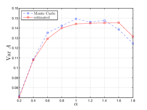
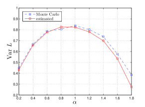
Figure 5 displays a study of the accuracy of Λ(A)Λsubscriptsuperscript𝐴\Lambda(A^{*}_{\bullet}) as an estimator. It plots Monte Carlo variances of the estimator 𝑬𝑬{\boldsymbol{E}} as well as their estimates Λ(A)Λsubscriptsuperscript𝐴\Lambda(A^{*}_{\bullet}) for several values of the parameter α𝛼\alpha. The latter nearly perfectly match the former in the subdiffusive range. A slight deviation appears in the strongly superdiffusive range, but still within an acceptable margin.
Refer to caption
Refer to caption
Figure 5: Comparative analysis of the standard error of the estimator 𝑬=(L,A)𝑬𝐿𝐴{\boldsymbol{E}}=(L,A) (dashed line; see (29)) and its AMSD-type estimator Λ(A)Λsuperscript𝐴\Lambda(A^{*}) (solid line; see (44)) as a function of the diffusion exponent α𝛼\alpha. The latter closely matches the former, especially in the subdiffusive range α<1𝛼1\alpha<1. The number of Monte Carlo runs is 1000 based on particle paths of length 210superscript2102^{10}.

Hence, we define the standardized estimators

𝒁j=(Zj,1Zj,2)=νjΛ1/2(Aj)𝑬j,j=I,II.formulae-sequencesubscriptsuperscript𝒁𝑗subscriptsuperscript𝑍𝑗1subscriptsuperscript𝑍𝑗2subscript𝜈𝑗superscriptΛ12subscriptsuperscript𝐴𝑗subscriptsuperscript𝑬𝑗𝑗III{\boldsymbol{Z}}^{*}_{j}=\left(\begin{array}[]{c}Z^{*}_{j,1}\\ Z^{*}_{j,2}\\ \end{array}\right)=\sqrt{\nu_{j}}\Lambda^{-1/2}(A^{*}_{j}){\boldsymbol{E}}^{*}_{j},\quad j=\mathrm{I,II}.

In view of Proposition C.1, these estimators are also asymptotically normal for 0<α<3/20𝛼320<\alpha<3/2. Hence, let

T1=ZI,1ZII,12,T2=ZI,2ZII,22formulae-sequencesubscript𝑇1subscriptsuperscript𝑍I1subscriptsuperscript𝑍II12subscript𝑇2subscriptsuperscript𝑍I2subscriptsuperscript𝑍II22T_{1}=\frac{Z^{*}_{\mathrm{I},1}-Z^{*}_{\mathrm{II},1}}{\sqrt{2}},\quad T_{2}=\frac{Z^{*}_{\mathrm{I},2}-Z^{*}_{\mathrm{II},2}}{\sqrt{2}} (45)

be the associated test statistics. The rejection region is given by

Rinter:|T1|>zϵ/4or|T2|>zϵ/4,:subscript𝑅interformulae-sequencesubscript𝑇1subscript𝑧italic-ϵ4orsubscript𝑇2subscript𝑧italic-ϵ4R_{\textnormal{inter}}:\left|T_{1}\right|>z_{\epsilon/4}\quad\mathrm{or}\quad\left|T_{2}\right|>z_{\epsilon/4}, (46)

where zϵ/4subscript𝑧italic-ϵ4z_{\epsilon/4} is a standard Normal quantile (c.f. Table 4, row “interfluid”). In (46), the probability ϵ/4italic-ϵ4\epsilon/4 stems, first, from applying a Bonferroni-type correction to a double testing region (hence yielding ϵ/2italic-ϵ2\epsilon/2 significance level in each), and second, from the fact that in each region the test statistic distribution is two-sided.

To check the test’s size over finite samples, we produced a 2000-run Monte Carlo study based on two sets of 50 paths with the same diffusion exponent, where tests were conducted at significance level ϵ=0.05italic-ϵ0.05\epsilon=0.05. As shown in Figure 3, right plot, the rejection rate was close to 0.05, as expected.

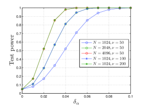
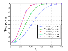
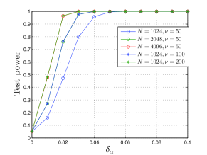
In Figure 6, we investigate the interfluid test power as a function of the path lengths and number of paths. The x𝑥x-axis represents the difference between the diffusion exponents from two fluids, namely,

δα=|αIαII|,subscript𝛿𝛼subscript𝛼Isubscript𝛼II\delta_{\alpha}=\left|\alpha_{\mathrm{I}}-\alpha_{\mathrm{II}}\right|, (47)

whereas the y𝑦y-axis is the test power at ϵ=0.05italic-ϵ0.05\epsilon=0.05. From top to bottom, the three plots correspond to αmin=min{αI,αII}=0.2,1.0,1.8formulae-sequencesubscript𝛼subscript𝛼Isubscript𝛼II0.21.01.8\alpha_{\min}=\min\{\alpha_{\mathrm{I}},\alpha_{\mathrm{II}}\}=0.2,1.0,1.8, respectively, for various combinations of realistic values of N𝑁N and ν=νI=νII𝜈subscript𝜈Isubscript𝜈II\nu=\nu_{\textnormal{I}}=\nu_{\textnormal{II}}. In all cases, the power curves start at around 0.05, as expected, and quickly approach 1 as a function of δαsubscript𝛿𝛼\delta_{\alpha} as defined in (47). Larger path lengths, larger number of particle paths as well as not very large values of αminsubscript𝛼\alpha_{\min} are associated with faster convergence of power curves to 1.
Refer to caption
Refer to caption
Refer to caption
Figure 6: Interfluid heterogeneity: test power. For various values of N𝑁N (see (2)) and ν=νI=νII𝜈subscript𝜈Isubscript𝜈II\nu=\nu_{\textnormal{I}}=\nu_{\textnormal{II}} (see (40)), we plot test power (y𝑦y-axis; see (32)) as a function of δαsubscript𝛿𝛼\delta_{\alpha} (x𝑥x-axis; see (47)). The parameter values are given by αmin:=min{αI,αII}assignsubscript𝛼subscript𝛼Isubscript𝛼II\alpha_{\min}:=\min\{\alpha_{\mathrm{I}},\alpha_{\mathrm{II}}\} in the range αmin=0.2,1.0,1.8subscript𝛼0.21.01.8\alpha_{\min}=0.2,1.0,1.8 (top, middle and bottom, respectively).

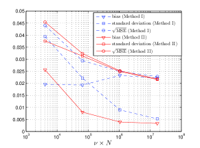
Interfluid heterogeneity: more or longer paths under technical–experimental constraints? Figure 6 also illustrates the following phenomenon. For the subdiffusive and diffusive cases, there is no visible difference between doubling the path lengths or the number of paths. However, in the strongly superdiffusive range, doubling the number of paths increases the test power more than doubling the path lengths.

In real world lab conditions, conducting single particle experiments involves coping with technical restrictions. For example, there may be limited camera recording time, tracer particles may slip out of the field of view or there may be a limit on the total number of tracer particles per fluid sample while still assuming that particles diffuse independently. So, assuming technical–experimental restrictions are in place, it is relevant to ask: what is the difference between

  • Method I: recording the movement of a larger number of particles (ν𝜈\nu) over a fixed period of time (hence, keeping constant the average sample path length N𝑁N); and

  • Method II: recording the same number of particles ν𝜈\nu over a longer period of time (hence, yielding a larger average N𝑁N)?

We answer this question in the framework of interfluid heterogeneity testing.

In the regimes of Methods I and II, we investigate the performance of the AMSD-type estimator (43) in terms of bias, standard deviation and square root MSE. Bearing in mind expression (42), by a similar reasoning to the one leading to expression (17) for a single observed path, the bias of log2MN(τ)subscript2subscriptsuperscript𝑀𝑁𝜏\log_{2}M^{*}_{N}(\tau) as an estimator of αlogτ+logσ2𝛼𝜏superscript𝜎2\alpha\log\tau+\log\sigma^{2} is given by

O(τδ)(MN(τ)X2(τ))22X2(τ)2=O(τδ)1ν(MN(τ)X2(τ))22X2(τ)2.𝑂superscript𝜏𝛿delimited-⟨⟩superscriptsubscriptsuperscript𝑀𝑁𝜏delimited-⟨⟩superscript𝑋2𝜏22superscriptdelimited-⟨⟩superscript𝑋2𝜏2𝑂superscript𝜏𝛿1𝜈delimited-⟨⟩superscriptsubscript𝑀𝑁𝜏delimited-⟨⟩superscript𝑋2𝜏22superscriptdelimited-⟨⟩superscript𝑋2𝜏2O(\tau^{-\delta})-\bigg{\langle}\frac{(M^{*}_{N}(\tau)-\langle X^{2}(\tau)\rangle)^{2}}{2\langle X^{2}(\tau)\rangle^{2}}\bigg{\rangle}=O(\tau^{-\delta})-\frac{1}{\nu}\bigg{\langle}\frac{(M_{N}(\tau)-\langle X^{2}(\tau)\rangle)^{2}}{2\langle X^{2}(\tau)\rangle^{2}}\bigg{\rangle}. (48)

Moreover, by the independence of particle paths, we can approximate the variance of log2MN(τ)subscript2subscriptsuperscript𝑀𝑁𝜏\log_{2}M^{*}_{N}(\tau) by

Var(logMN(τ))VarMN(τ)νX2(τ)4.Varsubscriptsuperscript𝑀𝑁𝜏Varsubscript𝑀𝑁𝜏𝜈superscriptdelimited-⟨⟩superscript𝑋2𝜏4{\mathrm{Var}}\Big{(}\log M^{*}_{N}(\tau)\Big{)}\approx\frac{{\mathrm{Var}}\hskip 2.84526ptM_{N}(\tau)}{\nu\langle X^{2}(\tau)\rangle^{4}}. (49)

The performance of the estimator (43) in the two regimes depends on the interplay between the bias and variance components (48) and (49), respectively. In a computational experiment, we applied the following procedure.

  • 1.

    Start out in the same setting: 24superscript242^{4} paths of length 28superscript282^{8} for each method, run 500 Monte Carlo simulations to get the bias, standard deviation and square root MSE of A𝐴A for Method I and II;

  • 2.

    for Method I, fix the path length and at each step generate 24superscript242^{4} times the previous number of paths and redo the Monte Carlos experiments;

  • 3.

    for Method II, fix the number of paths and at each step generate paths of length 24superscript242^{4} times the previous length, multiply all lags by 2 and redo the Monte Carlos experiments;

  • 4.

    repeat 2. and 3. three times.

For ease of comparison, Table 5 displays the multiple instances generated. Note that, at each step, the total number of points recorded

ν×N𝜈𝑁\nu\times N (50)

is identical for the two methods.

Method I Method II
step N𝑁N ν𝜈\nu ν×N𝜈𝑁\nu\times N N𝑁N ν𝜈\nu ν×N𝜈𝑁\nu\times N
1 28superscript282^{8} 24superscript242^{4} 212superscript2122^{12} 28superscript282^{8} 24superscript242^{4} 212superscript2122^{12}
2 28superscript282^{8} 28superscript282^{8} 216superscript2162^{16} 212superscript2122^{12} 24superscript242^{4} 216superscript2162^{16}
3 28superscript282^{8} 212superscript2122^{12} 220superscript2202^{20} 216superscript2162^{16} 24superscript242^{4} 220superscript2202^{20}
4 28superscript282^{8} 216superscript2162^{16} 224superscript2242^{24} 220superscript2202^{20} 24superscript242^{4} 224superscript2242^{24}
Table 5: Methods I and II.

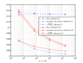
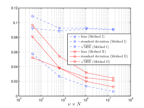
We compare the results in Figure 7, top and middle plots, where the diffusion exponent is set to α=0.6𝛼0.6\alpha=0.6 and 1.0, respectively. Method II has smaller bias and square root MSE. The reason is that, when ν𝜈\nu is large enough, the term O(τδ)𝑂superscript𝜏𝛿O(\tau^{-\delta}) dominates the bias. Thus, increasing the number of paths ν𝜈\nu does not reduce the bias. However, increasing the path length N𝑁N means that the TAMSD terms MN(τ)subscript𝑀𝑁𝜏M_{N}(\tau) with larger lag values τ𝜏\tau can be used in the regression procedure. This implies a reduction in magnitude of the term O(τδ)𝑂superscript𝜏𝛿O(\tau^{-\delta}), and hence, smaller bias. Method I displays smaller standard deviation because a 16-fold increase in ν𝜈\nu reduces the standard error by a factor of 1/4141/4. Meanwhile, noting that X2(τ)σ2ταsimilar-todelimited-⟨⟩superscript𝑋2𝜏superscript𝜎2superscript𝜏𝛼\langle X^{2}(\tau)\rangle\sim\sigma^{2}\tau^{\alpha}, expression (55) implies that for Method II the standard deviation is proportional to τ/N𝜏𝑁\sqrt{\tau/N}. By multiplying N𝑁N by 16 and τ𝜏\tau by 2, the standard error is reduced by a factor of 1/221221/2\sqrt{2}.

In Figure 7, bottom plot, we set α=1.8𝛼1.8\alpha=1.8. For this parameter value, the convergence rate of the TAMSD-based estimators is slower than 1N1𝑁\frac{1}{\sqrt{N}}. Method II still shows a smaller bias by comparison to Method I, as expected. However, since δ𝛿\delta increases as a function of α𝛼\alpha (see expression (54)), then O(τδ)𝑂superscript𝜏𝛿O(\tau^{-\delta}) shrinks with α𝛼\alpha. Therefore, the component O(τδ)𝑂superscript𝜏𝛿O(\tau^{-\delta}) carries less weight in the estimator’s bias for the superdiffusive case than for the subdiffusive case. Since α>3/2𝛼32\alpha>3/2, again by expression (55) (see also Remark 3.2) the standard deviation for Method II is proportional to (τ/N)2α=(τ/N)0.2superscript𝜏𝑁2𝛼superscript𝜏𝑁0.2(\tau/N)^{2-\alpha}=(\tau/N)^{0.2}. Thus, again assuming a 16-fold increase in N𝑁N and a 2-fold increase in τ𝜏\tau, the standard error is reduced by a factor of 1/80.21superscript80.21/8^{0.2}, which is much slower than the standard error reduction factor of 1/221221/2\sqrt{2} for Method I. These are the two reasons why Method I displays smaller square root MSE than Method II.
Refer to caption
Refer to caption
Refer to caption
Figure 7: Bias, standard deviation, and square root MSE for Methods I (blue) and II (red). The x𝑥x-axis denotes the total number of recorded data points (see (50)). Top: α=0.6𝛼0.6\alpha=0.6. Middle: α=1.0𝛼1.0\alpha=1.0. Bottom: α=1.8𝛼1.8\alpha=1.8.

5 Analysis of experimental data: heterogeneity of treated P. aeruginosa biofilms

The Hill and Schoenfisch Labs at UNC-Chapel Hill produced data from experiments on disruption and eradication of P. aeruginosa biofilms using nitric oxide-releasing chitosan oligosaccharides [73]. For the reader’s convenience, we provide a brief description of the experiments.

Cystic fibrosis (CF) lung disease is caused by defective chloride transport, resulting in thickened, dehydrated mucus. The latter restricts bacterial motility and promotes P. aeruginosa biofilm formation. Inhaled tobramycin is currently the only antibiotic recommended for the treatment of both initial and chronic P. aeruginosa infections in patients with CF. While inhaled tobramycin is effective at eradicating bacteria within biofilms, it fails to physically remove the structural remnants of the biofilm from the airways. This may lead to biofilm regrowth and the development of antibiotic-resistant infections. Therefore, an ideal anti-biofilm therapeutic for CF would both eradicate bacteria and physically degrade the biofilm, facilitating clearance from the airways.

On the other hand, nitric oxide (NO) is an endogenously produced diatomic free radical with significant antibacterial activity against P. aeruginosa biofilms. Atomic force microscopy revealed that NO exposure causes structural damage to the membranes of planktonic Gram-negative bacteria, including P. aeruginosa. The interest lies in the utility of NO-releasing chitosan oligosaccharides to both eradicate and physically alter P. aeruginosa biofilms and in comparing its effect with tobramycin. In order to measure the physical changes to bacterial biofilms caused by NO-releasing chitosan oligosaccharides, movements of fluorescent tracer particles embedded in P. aeruginosa biofilms were imaged at 60 frames per second for 30 seconds on an inverted microscope at 40×40\times magnification. The tracer particle displacement as a function of time was quantified using Video Spot Tracker software (Center for Computer Integrated Systems for Microscopy and Manipulation, University of North Carolina at Chapel Hill); see [73] for more details.

Fluid heterogeneity has been correlated with increased viscoelasticity for complex biological materials such as sputum [16]. In the experiments we describe, the effect of antibacterial treatment on biofilm heterogeneity was thus evaluated at different concentrations based on tracer particle displacement data. In Table 6, we use the data to test the intrafluid heterogeneity of P. aeruginosa biofilms after tobramycin treatments at concentrations levels 25, 50, 100, 200, and 400 μ𝜇\mug ml-1. From each of these fluid samples, we randomly select 100 paths of length N=1800𝑁1800N=1800. An application of the intrafluid test (38) produces strong evidence (negligible p𝑝p-values) of intrafluid heterogeneity in every sample. This conclusion matches those reported in [73]. Since no homogeneous fluid samples are detected from any of these five samples, we do not perform the interfluid heterogeneity test (46).

In Table 7, we apply (38) in the testing of intrafluid heterogeneity of P. aeruginosa biofilms after COS2-NO treatment at concentration levels 1, 2, 4, 8, and 16 mg ml-1. COS2 releases NO, which cause the physical disruption and eradication of biofilms [73], and also reduces the viscoelastic properties of mucus [72]. As before, 100 paths of length 1800 were randomly selected for each concentration level. At concentrations 1 or 2 mg ml-1, the p𝑝p-values are still less than machine error, which indicates strongly significant heterogeneity. As the concentration level increases to 4 and 8 mg ml-1, the p𝑝p-values also increase. At concentration level 16 mg ml-1, the p𝑝p-value reaches 0.18. Hence, we fail to reject the null hypothesis of intrafluid homogeneity. This provides evidence that the COS2-NO treatment is effective at eradicating P. aeruginosa biofilms. Once again, this analysis confirms the conclusions reported in [73]. In Table 8, by applying (46), we test the interfluid heterogeneity of P. aeruginosa biofilms after COS2-NO treatment at concentration level 16 mg ml-1. From each fluid sample (A, B and C), we selected 100 paths of length 1800 and conducted the test. It turns out that there is no evidence whatsoever of heterogeneity among fluid samples A, B and C.

Tobramycin (μ𝜇\mug ml-1) p𝑝p-value
25 <1016absentsuperscript1016<10^{-16}
50 <1016absentsuperscript1016<10^{-16}
100 <1016absentsuperscript1016<10^{-16}
200 <1016absentsuperscript1016<10^{-16}
400 <1016absentsuperscript1016<10^{-16}
Table 6: Intrafluid biofilm heterogeneity testing after treatment with tobramycin at concentration levels 25, 50, 100, 200, 400 μ𝜇\mug ml-1. 100 independent paths of length 1800 were randomly selected for each concentration level.
COS2-NO (mg ml-1) p𝑝p-value
1 <1016absentsuperscript1016<10^{-16}
2 <1016absentsuperscript1016<10^{-16}
4 2×10132superscript10132\times 10^{-13}
8 3×1093superscript1093\times 10^{-9}
16 0.18
Table 7: Intrafluid biofilm heterogeneity testing after treatment with COS2-NO at concentration levels 1, 2, 4, 8, 16 mg ml-1. 100 independent paths of length 1800 were randomly selected for each concentration level.
COS2-NO 16 mg ml-1 p𝑝p-value
Group A vs Group B 0.9996
Group A vs Group C 0.9998
Group B vs Group C 0.9999
Table 8: Interfluid biofilm heterogeneity testing after treatment with COS2-NO at concentration level 16 mg ml-1. 100 independent paths of length 1800 were randomly selected for each group.

6 Conclusion

Motivated by applications in viscoelastic diffusion, in this paper we start from the TAMSD’s asymptotic distribution for a broad class of Gaussian fractional stochastic processes [20] to propose statistical protocols that make use of single-particle tracking data in the detection of fluid heterogeneity.

The testing methodology is based on an improved TAMSD-type estimator. To construct this estimator, we tackle two of the main issues involved in TAMSD-based estimation, namely, we mathematically characterize: (a) the finite-sample bias in log-TAMSD-based methods; and (b) the effect of disturbance correlation. The theoretical results on (a) and (b) allow us to propose a nearly optimal estimator by combining a bias-correction procedure and a generalized least squares-type regression solution. The improved TAMSD-based estimator (29) is asymptotically normal for 0<α<3/20𝛼320<\alpha<3/2, and computational experiments show that the new estimator outperforms the standard TAMSD-based estimator both in terms of bias and square root MSE for values of α𝛼\alpha over the whole parameter range (0,2)02(0,2).

The estimator (29) is used in the construction of protocols for fluid heterogeneity detection in two different experimental situations, namely, when testing: (i)𝑖(i) whether different regions of the same fluid are heterogeneous (intrafluid heterogeneity); or (ii)𝑖𝑖(ii) whether two samples from each homogenous fluid are heterogeneous (interfluid heterogeneity). Reflecting the asymptotic behavior of (29), for 0<α<3/20𝛼320<\alpha<3/2 the test statistics (37) and (45) for intra- and interfluid heterogeneity are asymptotically chi-square and asymptotically normally distributed, respectively. This ensures the tests and associated quantiles are asymptotically valid. Computational experiments confirm that the tests’ significance levels are accurate over finite samples, and that the tests display high power even for relatively small deviations from the null hypotheses.

In all cases, for the sake of completeness, we discuss and provide computational studies on the strong superdiffusivity range 3/2α<232𝛼23/2\leq\alpha<2. Although this may not affect physical areas of application where subdiffusion is prevalent, this research points to one difficulty involved in TAMSD-based modeling, namely, a potentially non-Gaussian (Rosenblatt-type) limiting distribution with an intricate cumulant structure (cf. expression (60)).

The constructed framework helps to shed light on the effect of common technical experimental constraints such as limited camera recording time: we characterize the difference between observing longer particle paths and using a larger number of particle paths of given length.

We apply the protocols in physical practice by making inferences on fluid viscoelasticity with data from the Hill and Schoenfisch Labs (UNC-Chapel Hill), as first reported and described in [73]. The testing protocols reveal that COS2-NO treatment is effective in eradicating P. aeruginosa biofilms, since greater concentration levels of the treatment clearly lead to greater fluid homogeneity as detected by tracer particle displacement data.

The research contained in this paper points to a number of interesting questions. From a modeling standpoint, it would be convenient to construct a heterogeneity testing framework for single particle experiments that, unlike TAMSD-based methods, mathematically covers the full anomalous diffusion parametric range 0<α<20𝛼20<\alpha<2 under the same limit parametric family of distributions. Moreover, ideally a heterogeneity testing framework should be robust with respect to nuisance trends and added experimental noise. In another research direction, the same questions can be asked for classes of anomalous diffusion models not covered by the results in [20] such as, for example, continuous time random walks and related stochastic processes.

Appendix A The asymptotic distribution of the TAMSD

In Theorem A.1, we provide the asymptotic distribution of the TAMSD random vector after centering, which in Corollary A.1 allows developing the asymptotic distribution of the OLS estimator (7) of the diffusivity coefficient and diffusion exponent.

Theorem A.1.

(Didier and Zhang [20], Theorem 1) Suppose the particle motion is a Gaussian, stationary increment process whose covariance function admits the harmonizable (Fourier domain) representation

X(s)X(t)=Cα2(eisx1)(eitx1)x2f(x)𝑑x,α(0,2),Cα0.formulae-sequencedelimited-⟨⟩𝑋𝑠𝑋𝑡subscriptsuperscript𝐶2𝛼subscriptsuperscript𝑒𝑖𝑠𝑥1superscript𝑒𝑖𝑡𝑥1superscript𝑥2𝑓𝑥differential-d𝑥formulae-sequence𝛼02subscript𝐶𝛼0\langle X(s)X(t)\rangle=C^{2}_{\alpha}\int_{{\mathbb{R}}}\frac{(e^{isx}-1)(e^{-itx}-1)}{x^{2}}f(x)dx,\quad\alpha\in(0,2),\quad C_{\alpha}\neq 0. (51)

In (51), the spectral density has the generic form f(x)=s(x)|x|α/21/2𝑓𝑥𝑠𝑥superscript𝑥𝛼212f(x)=\frac{s(x)}{|x|^{\alpha/2-1/2}}, where the {\mathbb{C}}-valued high frequency function s(x)𝑠𝑥s(x) is bounded and satisfies the relations

|s(0)|2=1,||s(x)|21|C0|x|δ0,x(ε0,ε0),formulae-sequencesuperscript𝑠021formulae-sequencesuperscript𝑠𝑥21subscript𝐶0superscript𝑥subscript𝛿0𝑥subscript𝜀0subscript𝜀0\left|s(0)\right|^{2}=1,\quad|\left|s(x)\right|^{2}-1|\leq C_{0}|x|^{\delta_{0}},\quad x\in(-\varepsilon_{0},\varepsilon_{0}), (52)

for constants C0,δ0,ε0>0subscript𝐶0subscript𝛿0subscript𝜀00C_{0},\delta_{0},\varepsilon_{0}>0. Suppose the growth of the lag value term τ=τ(N)𝜏𝜏𝑁\tau=\tau(N)\in{\mathbb{N}} as in (15) with respect to the sample size N𝑁N is given by

τ(N)log2(N)N+Nτ(N)1+δ/20,N,formulae-sequence𝜏𝑁superscript2𝑁𝑁𝑁𝜏superscript𝑁1𝛿20𝑁\frac{\tau(N)\log^{2}(N)}{N}+\frac{N}{\tau(N)^{1+\delta/2}}\rightarrow 0,\quad N\rightarrow\infty, (53)

where

δ=min{α/2,δ0/2}.𝛿𝛼2subscript𝛿02\delta=\min\{\alpha/2,\delta_{0}/2\}. (54)

Also consider the rates of convergence

{0<α<3/2:η(N)=N,ζ(τ)=τα+1/2;α=3/2:η(N)=Nlog(N),ζ(τ)=τ2;3/2<α<2:η(N)=Nα1,ζ(τ)=τ2.cases:0𝛼32absentformulae-sequence𝜂𝑁𝑁𝜁𝜏superscript𝜏𝛼12missing-subexpression:𝛼32absentformulae-sequence𝜂𝑁𝑁𝑁𝜁𝜏superscript𝜏2missing-subexpression:32𝛼2absentformulae-sequence𝜂𝑁superscript𝑁𝛼1𝜁𝜏superscript𝜏2missing-subexpression\left\{\begin{array}[]{ccc}0<\alpha<3/2:&\eta(N)=\sqrt{N},\,\zeta(\tau)=\tau^{\alpha+1/2};\\ \alpha=3/2:&\eta(N)=\sqrt{N\log(N)},\,\zeta(\tau)=\tau^{2};\\ 3/2<\alpha<2:&\eta(N)=N^{\alpha-1},\,\zeta(\tau)=\tau^{2}.\end{array}\right. (55)

Then, as N𝑁N\rightarrow\infty,

(Nkη(Nk)ζ(τk)(MN(τk)X2(τk)))k=1,,md𝐙,superscript𝑑subscriptsubscript𝑁𝑘𝜂subscript𝑁𝑘𝜁subscript𝜏𝑘subscript𝑀𝑁subscript𝜏𝑘delimited-⟨⟩superscript𝑋2subscript𝜏𝑘𝑘1𝑚𝐙\bigg{(}\frac{N_{k}}{\eta(N_{k})\zeta(\tau_{k})}(M_{N}(\tau_{k})-\langle X^{2}(\tau_{k})\rangle)\bigg{)}_{k=1,\ldots,m}\stackrel{{\scriptstyle d}}{{\rightarrow}}{\mathbf{Z}}, (56)

where, for k=1,,m𝑘1𝑚k=1,\ldots,m, Nk=Nτksubscript𝑁𝑘𝑁subscript𝜏𝑘N_{k}=N-\tau_{k} is the number of available terms in each TAMSD sum (2) and τksubscript𝜏𝑘\tau_{k} is given by (15). In (56), the distribution of the random vector 𝐙𝐙{\mathbf{Z}} can be described as follows.

  • (i𝑖i)

    If 0<α<3/20𝛼320<\alpha<3/2, then 𝐙𝒩(0,Σ)similar-to𝐙𝒩0Σ{\mathbf{Z}}\sim{\mathcal{N}}(0,\Sigma) (a m𝑚m-variate Gaussian distribution), where the entry k1,k2subscript𝑘1subscript𝑘2k_{1},k_{2} of the matrix Σ=Σ(α)ΣΣ𝛼\Sigma=\Sigma(\alpha) is given by

    Σk1,k2=2wk1α1/2wk2α1/2(CαCH)4G^(y;wk1,wk2)L2()2,subscriptΣsubscript𝑘1subscript𝑘22superscriptsubscript𝑤subscript𝑘1𝛼12superscriptsubscript𝑤subscript𝑘2𝛼12superscriptsubscript𝐶𝛼subscript𝐶𝐻4subscriptsuperscriptnorm^𝐺𝑦subscript𝑤subscript𝑘1subscript𝑤subscript𝑘22superscript𝐿2\Sigma_{k_{1},k_{2}}=2w_{k_{1}}^{-\alpha-1/2}w_{k_{2}}^{-\alpha-1/2}\Big{(}\frac{C_{\alpha}}{C_{H}}\Big{)}^{4}\left\|\widehat{G}(y;w_{k_{1}},w_{k_{2}})\right\|^{2}_{L^{2}({\mathbb{R}})}, (57)

    k1,k2=1,,mformulae-sequencesubscript𝑘1subscript𝑘21𝑚k_{1},k_{2}=1,\ldots,m. In (57), we define

    CH=π1HΓ(2H)sin(Hπ)subscript𝐶𝐻superscript𝜋1𝐻Γ2𝐻𝐻𝜋C_{H}=\sqrt{\pi^{-1}H\Gamma(2H)\sin(H\pi)}

    and

    G^(y;wk1,wk2)=CH2(eiwk1y1)(eiwk2y1)|y|α+1;^𝐺𝑦subscript𝑤subscript𝑘1subscript𝑤subscript𝑘2subscriptsuperscript𝐶2𝐻superscript𝑒𝑖subscript𝑤subscript𝑘1𝑦1superscript𝑒𝑖subscript𝑤subscript𝑘2𝑦1superscript𝑦𝛼1\widehat{G}(y;w_{k_{1}},w_{k_{2}})=C^{2}_{H}\frac{(e^{iw_{k_{1}}y}-1)(e^{-iw_{k_{2}}y}-1)}{\left|y\right|^{\alpha+1}}; (58)
  • (ii𝑖𝑖ii)

    if α=3/2𝛼32\alpha=3/2, then 𝐙𝒩(0,Σ)similar-to𝐙𝒩0Σ{\mathbf{Z}}\sim{\mathcal{N}}(0,\Sigma), where the entry k1,k2subscript𝑘1subscript𝑘2k_{1},k_{2} of the matrix Σ=Σ(α)ΣΣ𝛼\Sigma=\Sigma(\alpha) is given by

    Σk1,k2=4ϑ2,k1,k2=1,,m,formulae-sequencesubscriptΣsubscript𝑘1subscript𝑘24superscriptitalic-ϑ2subscript𝑘1subscript𝑘21𝑚\Sigma_{k_{1},k_{2}}=4\vartheta^{2},\quad k_{1},k_{2}=1,\ldots,m, (59)

    and

    ϑ=(CαCH)2α(α1)2;italic-ϑsuperscriptsubscript𝐶𝛼subscript𝐶𝐻2𝛼𝛼12\vartheta=\bigg{(}\frac{C_{\alpha}}{C_{H}}\bigg{)}^{2}\frac{\alpha(\alpha-1)}{2};
  • (iii𝑖𝑖𝑖iii)

    if 3/2<α<232𝛼23/2<\alpha<2, 𝐙𝐙\mathbf{Z} follows a multivariate Rosenblatt-type distribution whose characteristic function is given by

    ϕ𝐙(𝐭)=exp{12s=2[2iϑk=1mtk]sscs(α)}subscriptitalic-ϕ𝐙𝐭12superscriptsubscript𝑠2superscriptdelimited-[]2𝑖italic-ϑsubscriptsuperscript𝑚𝑘1subscript𝑡𝑘𝑠𝑠subscript𝑐𝑠𝛼\phi_{\mathbf{Z}}({\mathbf{t}})=\exp\bigg{\{}\frac{1}{2}\sum_{s=2}^{\infty}\frac{[2i\vartheta\hskip 1.42262pt\sum^{m}_{k=1}t_{k}]^{s}}{s}\hskip 2.84526ptc_{s}(\alpha)\bigg{\}} (60)

    around the origin. In (60), for s2𝑠2s\geq 2, cs(α)subscript𝑐𝑠𝛼c_{s}(\alpha) is given by

    [0,1]s|x1x2|α2|x2x3|α2|xsx1|α2𝑑x1𝑑xs.subscriptsuperscript01𝑠superscriptsubscript𝑥1subscript𝑥2𝛼2superscriptsubscript𝑥2subscript𝑥3𝛼2superscriptsubscript𝑥𝑠subscript𝑥1𝛼2differential-dsubscript𝑥1differential-dsubscript𝑥𝑠\int_{[0,1]^{s}}|x_{1}-x_{2}|^{\alpha-2}|x_{2}-x_{3}|^{\alpha-2}\cdots|x_{s}-x_{1}|^{\alpha-2}dx_{1}\cdots dx_{s}. (61)

Consider again the regression system (20) and recall that expression (22) gives the standard estimator generated by the OLS solution to the system (20). The following corollary describes the asymptotic distribution of the standard estimator (22).

Corollary A.1.

(Didier and Zhang [20], Corollary 1) Suppose the assumptions of Theorem A.1 hold. Then, as N𝑁N\rightarrow\infty,

Nταη(N)ζ(τ)(1logτ(Lstandlogσ2)Astandα)d(UTUT)A𝐙.superscript𝑑𝑁superscript𝜏𝛼𝜂𝑁𝜁𝜏1𝜏subscript𝐿standsuperscript𝜎2subscript𝐴stand𝛼superscript𝑈𝑇superscript𝑈𝑇𝐴𝐙\frac{N\tau^{\alpha}}{\eta(N)\zeta(\tau)}\left(\begin{array}[]{c}\frac{1}{\log\tau}(L_{{\mathrm{stand}}}-{\log\sigma^{2}})\\ A_{{\mathrm{stand}}}-\alpha\\ \end{array}\right)\stackrel{{\scriptstyle d}}{{\rightarrow}}\left(\begin{array}[]{c}U^{T}\\ -U^{T}\\ \end{array}\right)A{\mathbf{Z}}. (62)

In (62),

A=A(σ2,α)=diag(ζ(w1)/(σ2w1α),,ζ(wm)/(σ2wmα)),𝐴𝐴superscript𝜎2𝛼diag𝜁subscript𝑤1superscript𝜎2superscriptsubscript𝑤1𝛼𝜁subscript𝑤𝑚superscript𝜎2superscriptsubscript𝑤𝑚𝛼A=A(\sigma^{2},\alpha)={\mathrm{diag}}(\zeta(w_{1})/(\sigma^{2}w_{1}^{\alpha}),\ldots,{\zeta(w_{m})}/(\sigma^{2}w_{m}^{\alpha})), (63)

η()𝜂\eta(\cdot), ζ()𝜁\zeta(\cdot) and 𝐙𝐙{\mathbf{Z}} are as in Theorem A.1, and

UT=1cw(k=1mlog(wk/w1),,k=1mlog(wk/wm))superscript𝑈𝑇1subscript𝑐𝑤superscriptsubscript𝑘1𝑚subscript𝑤𝑘subscript𝑤1superscriptsubscript𝑘1𝑚subscript𝑤𝑘subscript𝑤𝑚U^{T}=\frac{1}{c_{w}}\Big{(}\sum_{k=1}^{m}\log(w_{k}/w_{1}),\ldots,\sum_{k=1}^{m}\log(w_{k}/w_{m})\Big{)} (64)

with constant

cw=mk=1mlog2(wk)(k=1mlog(wk))2.subscript𝑐𝑤𝑚superscriptsubscript𝑘1𝑚superscript2subscript𝑤𝑘superscriptsuperscriptsubscript𝑘1𝑚subscript𝑤𝑘2c_{w}=m\sum_{k=1}^{m}\log^{2}(w_{k})-\Big{(}\sum_{k=1}^{m}\log(w_{k})\Big{)}^{2}. (65)

In particular, the standard estimator (22) is consistent, namely, relation (9) holds.

Proposition A.1.

(Didier and Zhang [20], Proposition 1, (i)𝑖(i)) Under the assumptions of Theorem A.1, there is a constant σ2>0superscript𝜎20\sigma^{2}>0 such that (16) holds for some C>0𝐶0C>0, where δ>0𝛿0\delta>0 is given by (54).

Appendix B Some lemmas

In this section, we present some lemmas that are used to prove Theorems C.1 and C.2 in Section C. Throughout this section, we assume 0<α<3/20𝛼320<\alpha<3/2 and the conditions of Theorem A.1. In proofs, whenever convenient C𝐶C denotes a constant that may change from one line to the next.

In light of (56), define the standardized statistic

ϖ(τ)=MN(τ)X2(τ).italic-ϖ𝜏subscript𝑀𝑁𝜏delimited-⟨⟩superscript𝑋2𝜏\varpi(\tau)=\frac{M_{N}(\tau)}{\langle X^{2}(\tau)\rangle}. (66)

In particular,

ϖ(τ)𝑃1,N,italic-ϖ𝜏𝑃1𝑁\varpi(\tau)\overset{P}{\rightarrow}1,\quad N\rightarrow\infty, (67)

so that a Taylor expansion can be applied to logϖ(τ)italic-ϖ𝜏\log\varpi(\tau) around 1. Meanwhile, we define the standardized increment

Wj(τ)=X(j+τ)X(j)X2(τ).subscript𝑊𝑗𝜏𝑋𝑗𝜏𝑋𝑗delimited-⟨⟩superscript𝑋2𝜏W_{j}(\tau)=\frac{X(j+\tau)-X(j)}{\sqrt{\langle X^{2}(\tau)\rangle}}. (68)

We will use the following results in our proofs. The first one is the classical Isserlis theorem, which reduces the higher moments of a multivariate normal vector to its second moments. The second one is a concentration inequality that will allow us to establish sharp bounds on the tails of centered quadratic forms.

Theorem B.1 (Isserlis, [37]).

Let (Z1,Z2,,Z2N)subscript𝑍1subscript𝑍2subscript𝑍2𝑁(Z_{1},Z_{2},\ldots,Z_{2N}) be a zero mean, multivariate normal random vector. Then,

Z1Z2Z2N=ZiZj,delimited-⟨⟩subscript𝑍1subscript𝑍2subscript𝑍2𝑁productdelimited-⟨⟩subscript𝑍𝑖subscript𝑍𝑗\langle Z_{1}Z_{2}\ldots Z_{2N}\rangle=\sum\prod\langle Z_{i}Z_{j}\rangle,

where the notation product\sum\prod stands for summing over all distinct ways of partitioning Z1,,Z2Nsubscript𝑍1subscript𝑍2𝑁Z_{1},\ldots,Z_{2N} into pairs Zi,Zjsubscript𝑍𝑖subscript𝑍𝑗Z_{i},Z_{j} and each summand is a product of these N𝑁N pairs.

Theorem B.2.

[47, 5] Let Z1,,ZNi.i.d.𝒩(0,1)Z_{1},\ldots,Z_{N}\overset{\mathrm{i.i.d.}}{\sim}{\mathcal{N}}(0,1) and consider constants η1,,ηN0subscript𝜂1subscript𝜂𝑁0\eta_{1},\ldots,\eta_{N}\geq 0, not all zero. Let 𝛈2subscriptnorm𝛈2\left\|\boldsymbol{\eta}\right\|_{2} and 𝛈subscriptnorm𝛈\left\|\boldsymbol{\eta}\right\|_{\infty} be the Euclidean square and sup norms of the vector 𝛈=(η1,,ηN)T𝛈superscriptsubscript𝜂1subscript𝜂𝑁𝑇\boldsymbol{\eta}=(\eta_{1},\ldots,\eta_{N})^{T}. Also, define the random variable X=i=1Nηi,N(Zi21)𝑋superscriptsubscript𝑖1𝑁subscript𝜂𝑖𝑁superscriptsubscript𝑍𝑖21X=\sum_{i=1}^{N}\eta_{i,N}(Z_{i}^{2}-1). Then, for every x>0𝑥0x>0,

(X2𝜼2x+2𝜼x)exp(x),𝑋2subscriptnorm𝜼2𝑥2subscriptnorm𝜼𝑥𝑥{\mathbb{P}}(X\geq 2\left\|\boldsymbol{\eta}\right\|_{2}\sqrt{x}+2\left\|\boldsymbol{\eta}\right\|_{\infty}x)\leq\exp(-x),
(X2𝜼2x)exp(x).𝑋2subscriptnorm𝜼2𝑥𝑥{\mathbb{P}}(X\leq-2\left\|\boldsymbol{\eta}\right\|_{2}\sqrt{x})\leq\exp(-x).

The following lemma describes some basic properties of the central moments of (66).

Lemma B.1.

As N𝑁N\rightarrow\infty,

(ϖ(τ)1)2=O(τN).delimited-⟨⟩superscriptitalic-ϖ𝜏12𝑂𝜏𝑁\langle(\varpi(\tau)-1)^{2}\rangle=O\Big{(}\frac{\tau}{N}\Big{)}. (69)

Moreover, any moment of ϖ(τ)1italic-ϖ𝜏1\varpi(\tau)-1 is bounded in N𝑁N, i.e.,

|(ϖ(τ)1)κ|=O(1),κ.formulae-sequencedelimited-⟨⟩superscriptitalic-ϖ𝜏1𝜅𝑂1𝜅\Big{|}\langle(\varpi(\tau)-1)^{\kappa}\rangle\Big{|}=O(1),\quad\kappa\in{\mathbb{N}}. (70)
Proof.

Expression (70) (for κ3𝜅3\kappa\geq 3) can be proved by adapting the argument for establishing expression (C.24) in [94], while making use of the bound (76) and Lemma B.2 (expressions (73) and (74)). So, for the reader’s convenience, we establish (69) (for κ=2𝜅2\kappa=2). The left-hand side of (69) can be rewritten as

1N2k1=1Nk2=1N((X(τ+k1)X(k1))2X2(τ)1)((X(τ+k1)X(k2))2X2(τ)1)1superscript𝑁2delimited-⟨⟩superscriptsubscriptsubscript𝑘11𝑁superscriptsubscriptsubscript𝑘21𝑁superscript𝑋𝜏subscript𝑘1𝑋subscript𝑘12delimited-⟨⟩superscript𝑋2𝜏1superscript𝑋𝜏subscript𝑘1𝑋subscript𝑘22delimited-⟨⟩superscript𝑋2𝜏1\frac{1}{N^{2}}\bigg{\langle}\sum_{k_{1}=1}^{N}\sum_{k_{2}=1}^{N}\bigg{(}\frac{(X(\tau+k_{1})-X(k_{1}))^{2}}{\langle X^{2}(\tau)\rangle}-1\bigg{)}\bigg{(}\frac{(X(\tau+k_{1})-X(k_{2}))^{2}}{\langle X^{2}(\tau)\rangle}-1\bigg{)}\bigg{\rangle}
=1N2k1=1Nk2=1N(Wk12(τ)1)(Wk22(τ)1).absent1superscript𝑁2delimited-⟨⟩superscriptsubscriptsubscript𝑘11𝑁superscriptsubscriptsubscript𝑘21𝑁superscriptsubscript𝑊subscript𝑘12𝜏1superscriptsubscript𝑊subscript𝑘22𝜏1=\frac{1}{N^{2}}\bigg{\langle}\sum_{k_{1}=1}^{N}\sum_{k_{2}=1}^{N}(W_{k_{1}}^{2}(\tau)-1)(W_{k_{2}}^{2}(\tau)-1)\bigg{\rangle}. (71)

By applying the Isserlis theorem (Theorem B.1),

(Wk12(τ)1)(Wk22(τ)1)=Wk12(τ)Wk22(τ)Wk12(τ)Wk22(τ)+1delimited-⟨⟩superscriptsubscript𝑊subscript𝑘12𝜏1superscriptsubscript𝑊subscript𝑘22𝜏1delimited-⟨⟩superscriptsubscript𝑊subscript𝑘12𝜏superscriptsubscript𝑊subscript𝑘22𝜏delimited-⟨⟩superscriptsubscript𝑊subscript𝑘12𝜏delimited-⟨⟩superscriptsubscript𝑊subscript𝑘22𝜏1\langle(W_{k_{1}}^{2}(\tau)-1)(W_{k_{2}}^{2}(\tau)-1)\rangle=\langle W_{k_{1}}^{2}(\tau)W_{k_{2}}^{2}(\tau)\rangle-\langle W_{k_{1}}^{2}(\tau)\rangle-\langle W_{k_{2}}^{2}(\tau)\rangle+1
=2Wk1(τ)Wk2(τ)2=2X2(τ)2γτ2(k1k2),absent2superscriptdelimited-⟨⟩subscript𝑊subscript𝑘1𝜏subscript𝑊subscript𝑘2𝜏22superscriptdelimited-⟨⟩superscript𝑋2𝜏2superscriptsubscript𝛾𝜏2subscript𝑘1subscript𝑘2=2\langle W_{k_{1}}(\tau)W_{k_{2}}(\tau)\rangle^{2}=\frac{2}{\langle X^{2}(\tau)\rangle^{2}}\gamma_{\tau}^{2}(k_{1}-k_{2}),

where

γh(k1k2)=(X(k1+h)X(k1))(X(k2+h)X(k2)).subscript𝛾subscript𝑘1subscript𝑘2delimited-⟨⟩𝑋subscript𝑘1𝑋subscript𝑘1𝑋subscript𝑘2𝑋subscript𝑘2\gamma_{h}(k_{1}-k_{2})=\langle(X(k_{1}+h)-X(k_{1}))(X(k_{2}+h)-X(k_{2}))\rangle.

Thus, (71) can be recast as

2N2X2(τ)2k1,k2=1Nγτ2(k1k2),2superscript𝑁2superscriptdelimited-⟨⟩superscript𝑋2𝜏2superscriptsubscriptsubscript𝑘1subscript𝑘21𝑁superscriptsubscript𝛾𝜏2subscript𝑘1subscript𝑘2\frac{2}{N^{2}\langle X^{2}(\tau)\rangle^{2}}\sum_{k_{1},k_{2}=1}^{N}\gamma_{\tau}^{2}(k_{1}-k_{2}), (72)

Note that

2N2X2(τ)2=O(1N2τ2α)=O(τNζ2(τ)η2(N)),2superscript𝑁2superscriptdelimited-⟨⟩superscript𝑋2𝜏2𝑂1superscript𝑁2superscript𝜏2𝛼𝑂𝜏𝑁superscript𝜁2𝜏superscript𝜂2𝑁\frac{2}{N^{2}\langle X^{2}(\tau)\rangle^{2}}=O\Big{(}\frac{1}{N^{2}\tau^{2\alpha}}\Big{)}=O\Big{(}\frac{\tau}{N}\zeta^{-2}(\tau)\eta^{-2}(N)\Big{)},

where ζ(τ),η(N)𝜁𝜏𝜂𝑁\zeta(\tau),\eta(N) are defined by (55). Then, by (72), Lemmas C.1 – C.4 in [20], expression (71) is of the order O(τN)𝑂𝜏𝑁O\Big{(}\frac{\tau}{N}\Big{)}, as claimed. ∎

The next lemma draws upon Theorem B.2 and Lemma B.1 to construct a concentration inequality for (66) (see also [22]).

Lemma B.2.

Fix <r<1/2<3/2<r𝑟1232superscript𝑟-\infty<r<1/2<3/2<r^{\prime}. Then, for any 0<ξ<1/20𝜉120<\xi<1/2 and some C>0𝐶0C>0,

(ϖ(τ)r)exp{C(Nτ)ξ}italic-ϖ𝜏𝑟𝐶superscript𝑁𝜏𝜉{\mathbb{P}}(\varpi(\tau)\leq r)\leq\exp\Big{\{}-C\Big{(}\frac{N}{\tau}\Big{)}^{\xi}\Big{\}} (73)

and

(ϖ(τ)r)exp{C(Nτ)ξ}.italic-ϖ𝜏superscript𝑟𝐶superscript𝑁𝜏𝜉{\mathbb{P}}(\varpi(\tau)\geq r^{\prime})\geq\exp\Big{\{}-C\Big{(}\frac{N}{\tau}\Big{)}^{\xi}\Big{\}}. (74)
Proof.

Let Wj(τ),j=1,,Nformulae-sequencesubscript𝑊𝑗𝜏𝑗1𝑁W_{j}(\tau),j=1,\ldots,N be as in (68). Then, for ϖ(τ)italic-ϖ𝜏\varpi(\tau) as in (67), we can write

ϖ(τ)=1Nj=1NWj2(τ)=1N𝐖NT𝐖N,italic-ϖ𝜏1𝑁superscriptsubscript𝑗1𝑁subscriptsuperscript𝑊2𝑗𝜏1𝑁superscriptsubscript𝐖𝑁𝑇subscript𝐖𝑁\varpi(\tau)=\frac{1}{N}\sum_{j=1}^{N}W^{2}_{j}(\tau)=\frac{1}{N}\mathbf{W}_{N}^{T}\mathbf{W}_{N},

where 𝐖N=(W1(τ),,WN(τ))Tsubscript𝐖𝑁superscriptsubscript𝑊1𝜏subscript𝑊𝑁𝜏𝑇\mathbf{W}_{N}=(W_{1}(\tau),\ldots,W_{N}(\tau))^{T} is a multivariate normal vector with covariance matrix ΓΓ\Gamma. Consider the spectral decomposition QΛQT=Γ𝑄Λsuperscript𝑄𝑇ΓQ\Lambda Q^{T}=\Gamma, where Q𝑄Q is a N×N𝑁𝑁N\times N orthogonal matrix and Λ=diag{λ1,,λN}Λdiagsubscript𝜆1subscript𝜆𝑁\Lambda={\mathrm{diag}}\{\lambda_{1},\ldots,\lambda_{N}\} is a N×N𝑁𝑁N\times N diagonal matrix. Then, 𝐖N=𝑑QΛ1/2𝐙Nsubscript𝐖𝑁𝑑𝑄superscriptΛ12subscript𝐙𝑁\mathbf{W}_{N}\overset{d}{=}Q\Lambda^{1/2}\mathbf{Z}_{N}, where 𝐙N=(Z1,,ZN)T𝒩(0,IN)subscript𝐙𝑁superscriptsubscript𝑍1subscript𝑍𝑁𝑇similar-to𝒩0subscript𝐼𝑁\mathbf{Z}_{N}=(Z_{1},\ldots,Z_{N})^{T}{\sim}{\mathcal{N}}(0,I_{N}), INsubscript𝐼𝑁I_{N} is the N×N𝑁𝑁N\times N identity matrix, and =𝑑𝑑\overset{d}{=} denotes equality in distribution. Therefore,

ϖ(τ)=𝑑1N(QΛ1/2𝐙N)TQΛ1/2𝐙N=1N𝐙NTΛ𝐙N=j=1Nηj,NZj2,italic-ϖ𝜏𝑑1𝑁superscript𝑄superscriptΛ12subscript𝐙𝑁𝑇𝑄superscriptΛ12subscript𝐙𝑁1𝑁superscriptsubscript𝐙𝑁𝑇Λsubscript𝐙𝑁superscriptsubscript𝑗1𝑁subscript𝜂𝑗𝑁superscriptsubscript𝑍𝑗2\varpi(\tau)\overset{d}{=}\frac{1}{N}(Q\Lambda^{1/2}\mathbf{Z}_{N})^{T}Q\Lambda^{1/2}\mathbf{Z}_{N}=\frac{1}{N}\mathbf{Z}_{N}^{T}\Lambda\mathbf{Z}_{N}=\sum_{j=1}^{N}\eta_{j,N}Z_{j}^{2}, (75)

where ηj,N=λjNsubscript𝜂𝑗𝑁subscript𝜆𝑗𝑁\eta_{j,N}=\frac{\lambda_{j}}{N}. Let 𝜼N=(ηi,N)i=1,,Nsubscript𝜼𝑁subscriptsubscript𝜂𝑖𝑁𝑖1𝑁\boldsymbol{\eta}_{N}=(\eta_{i,N})_{i=1,\ldots,N} be the vector of coefficients η,Nsubscript𝜂𝑁\eta_{\cdot,N}. By expression (69) in Lemma B.1,

𝜼N2𝜼N22=Varϖ(τ)=(ϖ(τ)1)2=O(τN).superscriptsubscriptnormsubscript𝜼𝑁2superscriptsubscriptnormsubscript𝜼𝑁22Varitalic-ϖ𝜏delimited-⟨⟩superscriptitalic-ϖ𝜏12𝑂𝜏𝑁\left\|\boldsymbol{\eta}_{N}\right\|_{\infty}^{2}\leq\left\|\boldsymbol{\eta}_{N}\right\|_{2}^{2}={\mathrm{Var}}\,\varpi(\tau)=\langle(\varpi(\tau)-1)^{2}\rangle=O\Big{(}\frac{\tau}{N}\Big{)}. (76)

By Theorem B.2, by using the same argument as in the proof of Lemma C.3 in [94], and applying the bound (76),

(ϖ(τ)r)=(j=1Nηj,N(Zj21)r1)exp{C𝜼N22}exp{CNτ}italic-ϖ𝜏𝑟superscriptsubscript𝑗1𝑁subscript𝜂𝑗𝑁superscriptsubscript𝑍𝑗21𝑟1𝐶superscriptsubscriptnormsubscript𝜼𝑁22𝐶𝑁𝜏{\mathbb{P}}(\varpi(\tau)\leq r)={\mathbb{P}}\Big{(}\sum_{j=1}^{N}\eta_{j,N}(Z_{j}^{2}-1)\leq r-1\Big{)}\leq\exp\bigg{\{}-\frac{C}{\left\|\boldsymbol{\eta}_{N}\right\|_{2}^{2}}\bigg{\}}\leq\exp\bigg{\{}-C\hskip 1.42262pt\frac{N}{\tau}\bigg{\}}

for some C>0𝐶0C>0. Thus, (73) follows. To show (74), it suffices to adapt the proof of expression (C.34) in [94]. In fact, by (76), 0<ξ<1/20𝜉120<\xi<1/2 and Theorem B.2,

(ϖ(τ)r)=(j=1Nηj,N(Zj21)r1)italic-ϖ𝜏superscript𝑟superscriptsubscript𝑗1𝑁subscript𝜂𝑗𝑁superscriptsubscript𝑍𝑗21superscript𝑟1{\mathbb{P}}(\varpi(\tau)\geq r^{\prime})={\mathbb{P}}\Big{(}\sum_{j=1}^{N}\eta_{j,N}(Z_{j}^{2}-1)\geq r^{\prime}-1\Big{)}
(j=1Nηj,N(Zj21)2𝜼N2(Nτ)ξ2+2𝜼N(Nτ)ξ)exp{C(Nτ)ξ}.absentsuperscriptsubscript𝑗1𝑁subscript𝜂𝑗𝑁superscriptsubscript𝑍𝑗212subscriptnormsubscript𝜼𝑁2superscript𝑁𝜏𝜉22subscriptnormsubscript𝜼𝑁superscript𝑁𝜏𝜉𝐶superscript𝑁𝜏𝜉\leq{\mathbb{P}}\Big{(}\sum_{j=1}^{N}\eta_{j,N}(Z_{j}^{2}-1)\geq 2\left\|\boldsymbol{\eta}_{N}\right\|_{2}\Big{(}\frac{N}{\tau}\Big{)}^{\frac{\xi}{2}}+2\left\|\boldsymbol{\eta}_{N}\right\|_{\infty}\Big{(}\frac{N}{\tau}\Big{)}^{\xi}\Big{)}\leq\exp\Big{\{}-C\Big{(}\frac{N}{\tau}\Big{)}^{\xi}\Big{\}}.

The following lemma is used in the proof of Lemma B.6.

Lemma B.3.

Let p1𝑝1p\geq 1, there is a constant Kpsubscript𝐾𝑝K_{p} only depending on p𝑝p such that

|logϖ(τ)|pKpdelimited-⟨⟩superscriptitalic-ϖ𝜏𝑝subscript𝐾𝑝\langle\left|\log\varpi(\tau)\right|^{p}\rangle\leq K_{p} (77)
Proof.

By (75), ϖ(τ)italic-ϖ𝜏\varpi(\tau) is a nonnegative weighted sum of independent chi-squared random variables, where not all weights are zero. Then, relation (77) is a consequence of expression (96) in [63], p. 184. ∎

The following lemma can be shown based on Lemma B.2 and an adaptation of the proof of expressions (C.38) and (C.39) in [94], which pertains to higher order (cross)moments of wavelet variance terms.

Lemma B.4.

Let κ1,κ2{0},κ1+κ23formulae-sequencesubscript𝜅1subscript𝜅20subscript𝜅1subscript𝜅23\kappa_{1},\kappa_{2}\in{\mathbb{N}}\cup\{0\},\kappa_{1}+\kappa_{2}\geq 3, and fix 0<r<1/20𝑟120<r<1/2. Then, as N𝑁N\rightarrow\infty,

(ϖ(τ1)1)κ1(ϖ(τ2)1)κ2=O[(τN)2].delimited-⟨⟩superscriptitalic-ϖsubscript𝜏11subscript𝜅1superscriptitalic-ϖsubscript𝜏21subscript𝜅2𝑂delimited-[]superscript𝜏𝑁2\langle(\varpi(\tau_{1})-1)^{\kappa_{1}}(\varpi(\tau_{2})-1)^{\kappa_{2}}\rangle=O\Big{[}\Big{(}\frac{\tau}{N}\Big{)}^{2}\Big{]}.
(ϖ(τ1)1)κ1(ϖ(τ2)1)κ21{min{ϖ(τ1),ϖ(τ2)}>r}=O[(τN)2].delimited-⟨⟩superscriptitalic-ϖsubscript𝜏11subscript𝜅1superscriptitalic-ϖsubscript𝜏21subscript𝜅2subscript1italic-ϖsubscript𝜏1italic-ϖsubscript𝜏2𝑟𝑂delimited-[]superscript𝜏𝑁2\langle(\varpi(\tau_{1})-1)^{\kappa_{1}}(\varpi(\tau_{2})-1)^{\kappa_{2}}1_{\{\min\{\varpi(\tau_{1}),\varpi(\tau_{2})\}>r\}}\rangle=O\Big{[}\Big{(}\frac{\tau}{N}\Big{)}^{2}\Big{]}. (78)

Lemmas B.5, B.6 and B.7, stated and shown next, are used in the proofs of Theorems C.1 and C.2. The lemmas provide expressions for (cross)moments and (cross)moments of logarithms of the random variables (66) at different lag values.

Lemma B.5.
(ϖ(τk1)1)(ϖ(τk2)1)=12ni=N+1N1(1|i|N)×\langle(\varpi(\tau_{k_{1}})-1)(\varpi(\tau_{k_{2}})-1)\rangle=\frac{1}{2n}\sum_{i=-N+1}^{N-1}\bigg{(}1-\frac{\left|i\right|}{N}\bigg{)}\times
×{|iτk1τk2+τk1τk2|α|iτk1τk2+τk1τk2τk2τk1|α\times\bigg{\{}\left|\frac{i}{\sqrt{\tau_{k_{1}}\tau_{k_{2}}}}+\sqrt{\frac{\tau_{k_{1}}}{\tau_{k_{2}}}}\right|^{\alpha}-\left|\frac{i}{\sqrt{\tau_{k_{1}}\tau_{k_{2}}}}+\sqrt{\frac{\tau_{k_{1}}}{\tau_{k_{2}}}}-\sqrt{\frac{\tau_{k_{2}}}{\tau_{k_{1}}}}\right|^{\alpha}-
|iτk1τk2|α+|iτk1τk2τk2τk1|α}2(1+O(τδ)).-\left|\frac{i}{\sqrt{\tau_{k_{1}}\tau_{k_{2}}}}\right|^{\alpha}+\left|\frac{i}{\sqrt{\tau_{k_{1}}\tau_{k_{2}}}}-\sqrt{\frac{\tau_{k_{2}}}{\tau_{k_{1}}}}\right|^{\alpha}\bigg{\}}^{2}(1+O(\tau^{-\delta})). (79)
Proof.

For notational simplicity, assume k1=1subscript𝑘11k_{1}=1 and k2=2subscript𝑘22k_{2}=2. By (68), the left-hand side of (79) can be rewritten as

1N2j1,j2=1N(Wj12(τ1)1)(Wj22(τ2)1)=1N2j1,j2=1NWj12(τ1)Wj22(τ2)1.1superscript𝑁2superscriptsubscriptsubscript𝑗1subscript𝑗21𝑁delimited-⟨⟩subscriptsuperscript𝑊2subscript𝑗1subscript𝜏11subscriptsuperscript𝑊2subscript𝑗2subscript𝜏211superscript𝑁2superscriptsubscriptsubscript𝑗1subscript𝑗21𝑁delimited-⟨⟩subscriptsuperscript𝑊2subscript𝑗1subscript𝜏1subscriptsuperscript𝑊2subscript𝑗2subscript𝜏21\frac{1}{N^{2}}\sum_{j_{1},j_{2}=1}^{N}\langle(W^{2}_{j_{1}}(\tau_{1})-1)(W^{2}_{j_{2}}(\tau_{2})-1)\rangle=\frac{1}{N^{2}}\sum_{j_{1},j_{2}=1}^{N}\langle W^{2}_{j_{1}}(\tau_{1})W^{2}_{j_{2}}(\tau_{2})\rangle-1. (80)

By Theorem B.1 (Isserlis),

Wj12(τ1)Wj22(τ2)=Wj12(τ1)Wj22(τ2)+2Wj1(τ1)Wj2(τ2)2delimited-⟨⟩subscriptsuperscript𝑊2subscript𝑗1subscript𝜏1subscriptsuperscript𝑊2subscript𝑗2subscript𝜏2delimited-⟨⟩subscriptsuperscript𝑊2subscript𝑗1subscript𝜏1delimited-⟨⟩subscriptsuperscript𝑊2subscript𝑗2subscript𝜏22superscriptdelimited-⟨⟩subscript𝑊subscript𝑗1subscript𝜏1subscript𝑊subscript𝑗2subscript𝜏22\langle W^{2}_{j_{1}}(\tau_{1})W^{2}_{j_{2}}(\tau_{2})\rangle=\langle W^{2}_{j_{1}}(\tau_{1})\rangle\langle W^{2}_{j_{2}}(\tau_{2})\rangle+2\langle W_{j_{1}}(\tau_{1})W_{j_{2}}(\tau_{2})\rangle^{2}
=1+2Wj1(τ1)Wj2(τ2)2.absent12superscriptdelimited-⟨⟩subscript𝑊subscript𝑗1subscript𝜏1subscript𝑊subscript𝑗2subscript𝜏22=1+2\langle W_{j_{1}}(\tau_{1})W_{j_{2}}(\tau_{2})\rangle^{2}. (81)

By Lemma A.1 in [20],

(X(j1+τ1)X(j1))(X(j2+τ2)X(j2))X2(τ1)X2(τ2)delimited-⟨⟩𝑋subscript𝑗1subscript𝜏1𝑋subscript𝑗1𝑋subscript𝑗2subscript𝜏2𝑋subscript𝑗2delimited-⟨⟩superscript𝑋2subscript𝜏1delimited-⟨⟩superscript𝑋2subscript𝜏2\bigg{\langle}\frac{(X(j_{1}+\tau_{1})-X(j_{1}))(X(j_{2}+\tau_{2})-X(j_{2}))}{\sqrt{\langle X^{2}(\tau_{1})\rangle}\sqrt{\langle X^{2}(\tau_{2})\rangle}}\bigg{\rangle}
=(BH(j1+τ1)BH(j1))(BH(j2+τ2)BH(j2))BH2(τ1)BH2(τ2)(1+O(τδ)),absentdelimited-⟨⟩subscript𝐵𝐻subscript𝑗1subscript𝜏1subscript𝐵𝐻subscript𝑗1subscript𝐵𝐻subscript𝑗2subscript𝜏2subscript𝐵𝐻subscript𝑗2delimited-⟨⟩superscriptsubscript𝐵𝐻2subscript𝜏1delimited-⟨⟩superscriptsubscript𝐵𝐻2subscript𝜏21𝑂superscript𝜏𝛿=\bigg{\langle}\frac{(B_{H}(j_{1}+\tau_{1})-B_{H}(j_{1}))(B_{H}(j_{2}+\tau_{2})-B_{H}(j_{2}))}{\sqrt{\langle B_{H}^{2}(\tau_{1})\rangle}\sqrt{\langle B_{H}^{2}(\tau_{2})\rangle}}\bigg{\rangle}(1+O(\tau^{-\delta})), (82)

where BHsubscript𝐵𝐻B_{H} is a standard fBm with Hurst parameter given by the relation (12). By (68), (82) and expression (10) for the covariance function of fBm,

Wj1(τ1)Wj2(τ2)=12{|j1j2τ1τ2+τ1τ2|α|j1j2τ1τ2+τ1τ2τ2τ1|α\langle W_{j_{1}}(\tau_{1})W_{j_{2}}(\tau_{2})\rangle=\frac{1}{2}\Big{\{}\left|\frac{j_{1}-j_{2}}{\sqrt{\tau_{1}\tau_{2}}}+\sqrt{\frac{\tau_{1}}{\tau_{2}}}\right|^{\alpha}-\left|\frac{j_{1}-j_{2}}{\sqrt{\tau_{1}\tau_{2}}}+\sqrt{\frac{\tau_{1}}{\tau_{2}}}-\sqrt{\frac{\tau_{2}}{\tau_{1}}}\right|^{\alpha}-
|j1j2τ1τ2|α+|j1j2τ1τ2τ2τ1|α}(1+O(τδ)).-\left|\frac{j_{1}-j_{2}}{\sqrt{\tau_{1}\tau_{2}}}\right|^{\alpha}+\left|\frac{j_{1}-j_{2}}{\sqrt{\tau_{1}\tau_{2}}}-\sqrt{\frac{\tau_{2}}{\tau_{1}}}\right|^{\alpha}\Big{\}}(1+O(\tau^{-\delta})). (83)

Since Wj1(τ1)Wj2(τ2)=Wj1+k(τ1)Wj2+k(τ2)delimited-⟨⟩subscript𝑊subscript𝑗1subscript𝜏1subscript𝑊subscript𝑗2subscript𝜏2delimited-⟨⟩subscript𝑊subscript𝑗1𝑘subscript𝜏1subscript𝑊subscript𝑗2𝑘subscript𝜏2\langle W_{j_{1}}(\tau_{1})W_{j_{2}}(\tau_{2})\rangle=\langle W_{j_{1}+k}(\tau_{1})W_{j_{2}+k}(\tau_{2})\rangle, then by expression (81) we can rewrite (80) as

12Ni=N+1N11Nj1j2=i,j1,j2=1N(2Wj1(τ1)Wj2(τ2))2.12𝑁superscriptsubscript𝑖𝑁1𝑁11𝑁superscriptsubscriptformulae-sequencesubscript𝑗1subscript𝑗2𝑖subscript𝑗1subscript𝑗21𝑁superscript2delimited-⟨⟩subscript𝑊subscript𝑗1subscript𝜏1subscript𝑊subscript𝑗2subscript𝜏22\frac{1}{2N}\sum_{i=-N+1}^{N-1}\frac{1}{N}\sum_{j_{1}-j_{2}=i,j_{1},j_{2}=1}^{N}(2\langle W_{j_{1}}(\tau_{1})W_{j_{2}}(\tau_{2})\rangle)^{2}. (84)

Relation (79) is now a consequence of (83) and (84). ∎

Lemma B.6.
logϖ(τk1)logϖ(τk2)=(ϖ(τk1)1)(ϖ(τk2)1)+o(τN).delimited-⟨⟩italic-ϖsubscript𝜏subscript𝑘1italic-ϖsubscript𝜏subscript𝑘2delimited-⟨⟩italic-ϖsubscript𝜏subscript𝑘11italic-ϖsubscript𝜏subscript𝑘21𝑜𝜏𝑁\langle\log\varpi(\tau_{k_{1}})\log\varpi(\tau_{k_{2}})\rangle=\langle(\varpi(\tau_{k_{1}})-1)(\varpi(\tau_{k_{2}})-1)\rangle+o\Big{(}\frac{\tau}{N}\Big{)}. (85)
Proof.

For notational simplicity, assume k1=1subscript𝑘11k_{1}=1 and k2=2subscript𝑘22k_{2}=2. Let

S1=logϖ(τ1)logϖ(τ2)logϖ(τ1)logϖ(τ2)1{min{ϖ(τ1),ϖ(τ2)}>r},subscript𝑆1delimited-⟨⟩italic-ϖsubscript𝜏1italic-ϖsubscript𝜏2delimited-⟨⟩italic-ϖsubscript𝜏1italic-ϖsubscript𝜏2subscript1italic-ϖsubscript𝜏1italic-ϖsubscript𝜏2𝑟S_{1}=\langle\log\varpi(\tau_{1})\log\varpi(\tau_{2})\rangle-\langle\log\varpi(\tau_{1})\log\varpi(\tau_{2})1_{\{\min\{\varpi(\tau_{1}),\varpi(\tau_{2})\}>r\}}\rangle,
S2=logϖ(τ1)logϖ(τ2)1{min{ϖ(τ1),ϖ(τ2)}>r}subscript𝑆2limit-fromdelimited-⟨⟩italic-ϖsubscript𝜏1italic-ϖsubscript𝜏2subscript1italic-ϖsubscript𝜏1italic-ϖsubscript𝜏2𝑟S_{2}=\langle\log\varpi(\tau_{1})\log\varpi(\tau_{2})1_{\{\min\{\varpi(\tau_{1}),\varpi(\tau_{2})\}>r\}}\rangle-
(ϖ(τ1)1)(ϖ(τ2)1)1{min{ϖ(τ1),ϖ(τ2)}>r},delimited-⟨⟩italic-ϖsubscript𝜏11italic-ϖsubscript𝜏21subscript1italic-ϖsubscript𝜏1italic-ϖsubscript𝜏2𝑟-\langle(\varpi(\tau_{1})-1)(\varpi(\tau_{2})-1)1_{\{\min\{\varpi(\tau_{1}),\varpi(\tau_{2})\}>r\}}\rangle,
S3=(ϖ(τ1)1)(ϖ(τ2)1)1{min{ϖ(τ1),ϖ(τ2)}>r}(ϖ(τ1)1)(ϖ(τ2)1).subscript𝑆3delimited-⟨⟩italic-ϖsubscript𝜏11italic-ϖsubscript𝜏21subscript1italic-ϖsubscript𝜏1italic-ϖsubscript𝜏2𝑟delimited-⟨⟩italic-ϖsubscript𝜏11italic-ϖsubscript𝜏21S_{3}=\langle(\varpi(\tau_{1})-1)(\varpi(\tau_{2})-1)1_{\{\min\{\varpi(\tau_{1}),\varpi(\tau_{2})\}>r\}}\rangle-\langle(\varpi(\tau_{1})-1)(\varpi(\tau_{2})-1)\rangle.

Note that

logϖ(τ1)logϖ(τ2)=S1+S2+S3.delimited-⟨⟩italic-ϖsubscript𝜏1italic-ϖsubscript𝜏2subscript𝑆1subscript𝑆2subscript𝑆3\langle\log\varpi(\tau_{1})\log\varpi(\tau_{2})\rangle=S_{1}+S_{2}+S_{3}.

Therefore, establishing (85) is equivalent to showing that S1+S2+S3=o(τN)subscript𝑆1subscript𝑆2subscript𝑆3𝑜𝜏𝑁S_{1}+S_{2}+S_{3}=o\Big{(}\frac{\tau}{N}\Big{)}. It suffices to show that

max{|S1|,|S2|,|S3|}=o(τN).subscript𝑆1subscript𝑆2subscript𝑆3𝑜𝜏𝑁\max\{|S_{1}|,|S_{2}|,|S_{3}|\}=o\Big{(}\frac{\tau}{N}\Big{)}. (86)

Let 0<r<1/20𝑟120<r<1/2. We start off with S2subscript𝑆2S_{2} by writing out the almost sure Taylor expansion

logϖ(τ)1{ϖ(τ)>r}={(ϖ(τ)1)12(ϖ(τ)1σ+2(ϖ(τ)))2}1{ϖ(τ)>r},italic-ϖ𝜏subscript1italic-ϖ𝜏𝑟italic-ϖ𝜏112superscriptitalic-ϖ𝜏1subscriptsuperscript𝜎2italic-ϖ𝜏2subscript1italic-ϖ𝜏𝑟\log\varpi(\tau)1_{\{\varpi(\tau)>r\}}=\bigg{\{}(\varpi(\tau)-1)-\frac{1}{2}\bigg{(}\frac{\varpi(\tau)-1}{\sigma^{2}_{+}(\varpi(\tau))}\bigg{)}^{2}\bigg{\}}1_{\{\varpi(\tau)>r\}}, (87)

where σ+2(ϖ(τ))[min{ϖ(τ),1},max{ϖ(τ),1}]subscriptsuperscript𝜎2italic-ϖ𝜏italic-ϖ𝜏1italic-ϖ𝜏1\sigma^{2}_{+}(\varpi(\tau))\in[\min\{\varpi(\tau),1\},\max\{\varpi(\tau),1\}]. Then,

logϖ(τ1)logϖ(τ2)1{min{ϖ(τ1),ϖ(τ2)}>r}delimited-⟨⟩italic-ϖsubscript𝜏1italic-ϖsubscript𝜏2subscript1italic-ϖsubscript𝜏1italic-ϖsubscript𝜏2𝑟\langle\log\varpi(\tau_{1})\log\varpi(\tau_{2})1_{\{\min\{\varpi(\tau_{1}),\varpi(\tau_{2})\}>r\}}\rangle
=(ϖ(τ1)1)(ϖ(τ2)1)1{min{ϖ(τ1),ϖ(τ2)}>r}absentdelimited-⟨⟩italic-ϖsubscript𝜏11italic-ϖsubscript𝜏21subscript1italic-ϖsubscript𝜏1italic-ϖsubscript𝜏2𝑟=\langle(\varpi(\tau_{1})-1)(\varpi(\tau_{2})-1)1_{\{\min\{\varpi(\tau_{1}),\varpi(\tau_{2})\}>r\}}\rangle
12(ϖ(τ1)1)(ϖ(τ2)1σ+2(ϖ(τ2)))21{min{ϖ(τ1),ϖ(τ2)}>r}12delimited-⟨⟩italic-ϖsubscript𝜏11superscriptitalic-ϖsubscript𝜏21subscriptsuperscript𝜎2italic-ϖsubscript𝜏22subscript1italic-ϖsubscript𝜏1italic-ϖsubscript𝜏2𝑟-\frac{1}{2}\bigg{\langle}(\varpi(\tau_{1})-1)\bigg{(}\frac{\varpi(\tau_{2})-1}{\sigma^{2}_{+}(\varpi(\tau_{2}))}\bigg{)}^{2}1_{\{\min\{\varpi(\tau_{1}),\varpi(\tau_{2})\}>r\}}\bigg{\rangle}
12(ϖ(τ1)1σ+2(ϖ(τ1)))2(ϖ(τ2)1)1{min{ϖ(τ1),ϖ(τ2)}>r}12delimited-⟨⟩superscriptitalic-ϖsubscript𝜏11subscriptsuperscript𝜎2italic-ϖsubscript𝜏12italic-ϖsubscript𝜏21subscript1italic-ϖsubscript𝜏1italic-ϖsubscript𝜏2𝑟-\frac{1}{2}\bigg{\langle}\bigg{(}\frac{\varpi(\tau_{1})-1}{\sigma^{2}_{+}(\varpi(\tau_{1}))}\bigg{)}^{2}(\varpi(\tau_{2})-1)1_{\{\min\{\varpi(\tau_{1}),\varpi(\tau_{2})\}>r\}}\bigg{\rangle}
+14(ϖ(τ1)1σ+2(ϖ(τ1)))2(ϖ(τ2)1σ+2(ϖ(τ2)))21{min{ϖ(τ1),ϖ(τ2)}>r}.14delimited-⟨⟩superscriptitalic-ϖsubscript𝜏11subscriptsuperscript𝜎2italic-ϖsubscript𝜏12superscriptitalic-ϖsubscript𝜏21subscriptsuperscript𝜎2italic-ϖsubscript𝜏22subscript1italic-ϖsubscript𝜏1italic-ϖsubscript𝜏2𝑟+\frac{1}{4}\bigg{\langle}\bigg{(}\frac{\varpi(\tau_{1})-1}{\sigma^{2}_{+}(\varpi(\tau_{1}))}\bigg{)}^{2}\bigg{(}\frac{\varpi(\tau_{2})-1}{\sigma^{2}_{+}(\varpi(\tau_{2}))}\bigg{)}^{2}1_{\{\min\{\varpi(\tau_{1}),\varpi(\tau_{2})\}>r\}}\bigg{\rangle}. (88)

The second, third and fourth terms can be bounded by a similar argument, so we only develop the latter. Recast

(ϖ(τ)1σ+2(ϖ(τ)))21{ϖ(τ)>r}=(ϖ(τ)1σ+2(ϖ(τ)))2(1{1/2>ϖ(τ)>r}+1{ϖ(τ)1/2})superscriptitalic-ϖ𝜏1subscriptsuperscript𝜎2italic-ϖ𝜏2subscript1italic-ϖ𝜏𝑟superscriptitalic-ϖ𝜏1subscriptsuperscript𝜎2italic-ϖ𝜏2subscript112italic-ϖ𝜏𝑟subscript1italic-ϖ𝜏12\bigg{(}\frac{\varpi(\tau)-1}{\sigma^{2}_{+}(\varpi(\tau))}\bigg{)}^{2}1_{\{\varpi(\tau)>r\}}=\bigg{(}\frac{\varpi(\tau)-1}{\sigma^{2}_{+}(\varpi(\tau))}\bigg{)}^{2}\bigg{(}1_{\{1/2>\varpi(\tau)>r\}}+1_{\{\varpi(\tau)\geq 1/2\}}\bigg{)}
(ϖ(τ)1r)21{1/2>ϖ(τ)>r}+(ϖ(τ)11/2)21{ϖ(τ)1/2}.absentsuperscriptitalic-ϖ𝜏1𝑟2subscript112italic-ϖ𝜏𝑟superscriptitalic-ϖ𝜏1122subscript1italic-ϖ𝜏12\leq\bigg{(}\frac{\varpi(\tau)-1}{r}\bigg{)}^{2}1_{\{1/2>\varpi(\tau)>r\}}+\bigg{(}\frac{\varpi(\tau)-1}{1/2}\bigg{)}^{2}1_{\{\varpi(\tau)\geq 1/2\}}. (89)

Therefore, we can rewrite the fourth term in (88) as

(ϖ(τ1)1σ+2(ϖ(τ1)))2(ϖ(τ2)1σ+2(ϖ(τ2)))21{min{ϖ(τ1),ϖ(τ2)}>r}delimited-⟨⟩superscriptitalic-ϖsubscript𝜏11subscriptsuperscript𝜎2italic-ϖsubscript𝜏12superscriptitalic-ϖsubscript𝜏21subscriptsuperscript𝜎2italic-ϖsubscript𝜏22subscript1italic-ϖsubscript𝜏1italic-ϖsubscript𝜏2𝑟\bigg{\langle}\bigg{(}\frac{\varpi(\tau_{1})-1}{\sigma^{2}_{+}(\varpi(\tau_{1}))}\bigg{)}^{2}\bigg{(}\frac{\varpi(\tau_{2})-1}{\sigma^{2}_{+}(\varpi(\tau_{2}))}\bigg{)}^{2}1_{\{\min\{\varpi(\tau_{1}),\varpi(\tau_{2})\}>r\}}\bigg{\rangle}
1r4(ϖ(τ1)1)21{1/2>ϖ(τ1)>r}(ϖ(τ2)1)21{1/2>ϖ(τ2)>r}absent1superscript𝑟4delimited-⟨⟩superscriptitalic-ϖsubscript𝜏112subscript112italic-ϖsubscript𝜏1𝑟superscriptitalic-ϖsubscript𝜏212subscript112italic-ϖsubscript𝜏2𝑟\leq\frac{1}{r^{4}}\langle(\varpi(\tau_{1})-1)^{2}1_{\{1/2>\varpi(\tau_{1})>r\}}(\varpi(\tau_{2})-1)^{2}1_{\{1/2>\varpi(\tau_{2})>r\}}\rangle
+1(r/2)2(ϖ(τ1)1)21{ϖ(τ1)1/2}(ϖ(τ2)1)21{1/2>ϖ(τ2)>r}1superscript𝑟22delimited-⟨⟩superscriptitalic-ϖsubscript𝜏112subscript1italic-ϖsubscript𝜏112superscriptitalic-ϖsubscript𝜏212subscript112italic-ϖsubscript𝜏2𝑟+\frac{1}{(r/2)^{2}}\langle(\varpi(\tau_{1})-1)^{2}1_{\{\varpi(\tau_{1})\geq 1/2\}}(\varpi(\tau_{2})-1)^{2}1_{\{1/2>\varpi(\tau_{2})>r\}}\rangle
+1(r/2)2(ϖ(τ1)1)21{1/2>ϖ(τ2)>r}(ϖ(τ2)1)21{ϖ(τ2)1/2}1superscript𝑟22delimited-⟨⟩superscriptitalic-ϖsubscript𝜏112subscript112italic-ϖsubscript𝜏2𝑟superscriptitalic-ϖsubscript𝜏212subscript1italic-ϖsubscript𝜏212+\frac{1}{(r/2)^{2}}\langle(\varpi(\tau_{1})-1)^{2}1_{\{1/2>\varpi(\tau_{2})>r\}}(\varpi(\tau_{2})-1)^{2}1_{\{\varpi(\tau_{2})\geq 1/2\}}\rangle
+1(1/2)4(ϖ(τ1)1)21{ϖ(τ2)1/2}(ϖ(τ2)1)21{ϖ(τ2)1/2}1superscript124delimited-⟨⟩superscriptitalic-ϖsubscript𝜏112subscript1italic-ϖsubscript𝜏212superscriptitalic-ϖsubscript𝜏212subscript1italic-ϖsubscript𝜏212+\frac{1}{(1/2)^{4}}\langle(\varpi(\tau_{1})-1)^{2}1_{\{\varpi(\tau_{2})\geq 1/2\}}(\varpi(\tau_{2})-1)^{2}1_{\{\varpi(\tau_{2})\geq 1/2\}}\rangle (90)

By (78), the fourth term in (90) is bounded by

O[(τN)2].𝑂delimited-[]superscript𝜏𝑁2O\Big{[}\Big{(}\frac{\tau}{N}\Big{)}^{2}\Big{]}. (91)

By the Cauchy-Schwarz inequality, (73) and (78), the first term in the sum (90) is bounded by

1r4(ϖ(τ1)1)4(ϖ(τ1)1)41{1/2>ϖ(τ1)>r}1{1/2>ϖ(τ2)>r}1superscript𝑟4delimited-⟨⟩superscriptitalic-ϖsubscript𝜏114superscriptitalic-ϖsubscript𝜏114delimited-⟨⟩subscript112italic-ϖsubscript𝜏1𝑟subscript112italic-ϖsubscript𝜏2𝑟\frac{1}{r^{4}}\sqrt{\langle(\varpi(\tau_{1})-1)^{4}(\varpi(\tau_{1})-1)^{4}\rangle}\sqrt{\langle 1_{\{1/2>\varpi(\tau_{1})>r\}}1_{\{1/2>\varpi(\tau_{2})>r\}}\rangle}
1r4O(τN)(1/2>ϖ(τ1)>r)(1/2>ϖ(τ2)>r)absent1superscript𝑟4𝑂𝜏𝑁12italic-ϖsubscript𝜏1𝑟12italic-ϖsubscript𝜏2𝑟\leq\frac{1}{r^{4}}O\Big{(}\frac{\tau}{N}\Big{)}\sqrt{{\mathbb{P}}(1/2>\varpi(\tau_{1})>r){\mathbb{P}}(1/2>\varpi(\tau_{2})>r)}
1r4O(τN)exp{C(Nτ)1ξ}=o(τN).absent1superscript𝑟4𝑂𝜏𝑁𝐶superscript𝑁𝜏1𝜉𝑜𝜏𝑁\leq\frac{1}{r^{4}}O\Big{(}\frac{\tau}{N}\Big{)}\exp\Big{\{}-C\Big{(}\frac{N}{\tau}\Big{)}^{1-\xi}\Big{\}}=o\Big{(}\frac{\tau}{N}\Big{)}. (92)

Again by the Cauchy-Schwarz inequality, (73) and (78), the second term in the sum (90) is bounded by

4r2(ϖ(τ1)1)4(ϖ(τ1)1)41{ϖ(τ1)1/2}1{1/2>ϖ(τ2)>r}4superscript𝑟2delimited-⟨⟩superscriptitalic-ϖsubscript𝜏114superscriptitalic-ϖsubscript𝜏114delimited-⟨⟩subscript1italic-ϖsubscript𝜏112subscript112italic-ϖsubscript𝜏2𝑟\frac{4}{r^{2}}\sqrt{\langle(\varpi(\tau_{1})-1)^{4}(\varpi(\tau_{1})-1)^{4}\rangle}\sqrt{\langle 1_{\{\varpi(\tau_{1})\geq 1/2\}}1_{\{1/2>\varpi(\tau_{2})>r\}}\rangle}
4r2O(τN)(ϖ(τ1)1/2)(1/2>ϖ(τ2)>r)absent4superscript𝑟2𝑂𝜏𝑁italic-ϖsubscript𝜏11212italic-ϖsubscript𝜏2𝑟\leq\frac{4}{r^{2}}O\Big{(}\frac{\tau}{N}\Big{)}\sqrt{{\mathbb{P}}(\varpi(\tau_{1})\geq 1/2){\mathbb{P}}(1/2>\varpi(\tau_{2})>r)}
4r2O(τN)exp{C(Nτ)1ξ}=o(τN).absent4superscript𝑟2𝑂𝜏𝑁𝐶superscript𝑁𝜏1𝜉𝑜𝜏𝑁\leq\frac{4}{r^{2}}O\Big{(}\frac{\tau}{N}\Big{)}\exp\Big{\{}-C\Big{(}\frac{N}{\tau}\Big{)}^{1-\xi}\Big{\}}=o\Big{(}\frac{\tau}{N}\Big{)}. (93)

An analogous bound holds for the third term in the sum (90). Therefore, |S2|subscript𝑆2|S_{2}| is bounded by the right-hand side of (86). To tackle S3subscript𝑆3S_{3}, rewrite it as

(ϖ(τ1)1)(ϖ(τ2)1)(1{ϖ(τ1)>r}1{ϖ(τ2)r}-\langle(\varpi(\tau_{1})-1)(\varpi(\tau_{2})-1)(1_{\{\varpi(\tau_{1})>r\}}1_{\{\varpi(\tau_{2})\leq r\}}
+1{ϖ(τ1)r}1{ϖ(τ2)>r}+1{ϖ(τ1)r}1{ϖ(τ2)r}).+1_{\{\varpi(\tau_{1})\leq r\}}1_{\{\varpi(\tau_{2})>r\}}+1_{\{\varpi(\tau_{1})\leq r\}}1_{\{\varpi(\tau_{2})\leq r\}})\rangle. (94)

By the Cauchy-Schwarz inequality, (73) and (78), the first term on the right-hand side of (94) is bounded by

(ϖ(τ1)1)2(ϖ(τ2)1)2(ϖ(τ2)r)delimited-⟨⟩superscriptitalic-ϖsubscript𝜏112superscriptitalic-ϖsubscript𝜏212italic-ϖsubscript𝜏2𝑟\sqrt{\langle(\varpi(\tau_{1})-1)^{2}(\varpi(\tau_{2})-1)^{2}\rangle}\sqrt{{\mathbb{P}}(\varpi(\tau_{2})\leq r)}
O(τN)exp{C(Nτ)1ξ}=o(τN).absent𝑂𝜏𝑁𝐶superscript𝑁𝜏1𝜉𝑜𝜏𝑁\leq O\Big{(}\frac{\tau}{N}\Big{)}\exp\Big{\{}-C\Big{(}\frac{N}{\tau}\Big{)}^{1-\xi}\Big{\}}=o\Big{(}\frac{\tau}{N}\Big{)}.

Similar bounds hold for the remaining terms on the right-hand side of (94). Therefore, |S3|subscript𝑆3|S_{3}| is also bounded by the right-hand side of (86). As for S1subscript𝑆1S_{1}, it can be reexpressed as

logϖ(τ1)logϖ(τ2)(1{ϖ(τ1)>r}1{ϖ(τ2)r}+1{ϖ(τ1)r}1{ϖ(τ2)>r}+1{ϖ(τ1)r}1{ϖ(τ2)r}).delimited-⟨⟩italic-ϖsubscript𝜏1italic-ϖsubscript𝜏2subscript1italic-ϖsubscript𝜏1𝑟subscript1italic-ϖsubscript𝜏2𝑟subscript1italic-ϖsubscript𝜏1𝑟subscript1italic-ϖsubscript𝜏2𝑟subscript1italic-ϖsubscript𝜏1𝑟subscript1italic-ϖsubscript𝜏2𝑟\langle\log\varpi(\tau_{1})\log\varpi(\tau_{2})\Big{(}1_{\{\varpi(\tau_{1})>r\}}1_{\{\varpi(\tau_{2})\leq r\}}+1_{\{\varpi(\tau_{1})\leq r\}}1_{\{\varpi(\tau_{2})>r\}}+1_{\{\varpi(\tau_{1})\leq r\}}1_{\{\varpi(\tau_{2})\leq r\}}\Big{)}\rangle. (95)

Note that, by Lemma B.3, log4ϖ(τ)delimited-⟨⟩superscript4italic-ϖ𝜏\langle\log^{4}\varpi(\tau)\rangle is bounded. Then, by applying the Cauchy-Schwarz inequality twice, the first term on the right-hand side of (95) is bounded by

log2ϖ(τ1)log2ϖ(τ2)(ϖ(τ2)r)delimited-⟨⟩superscript2italic-ϖsubscript𝜏1superscript2italic-ϖsubscript𝜏2italic-ϖsubscript𝜏2𝑟\sqrt{\langle\log^{2}\varpi(\tau_{1})\log^{2}\varpi(\tau_{2})\rangle}\sqrt{{\mathbb{P}}(\varpi(\tau_{2})\leq r)}
(log4ϖ(τ1)log4ϖ(τ2))1/4exp{C(Nτ)1ξ}=o(τN).absentsuperscriptdelimited-⟨⟩superscript4italic-ϖsubscript𝜏1delimited-⟨⟩superscript4italic-ϖsubscript𝜏214𝐶superscript𝑁𝜏1𝜉𝑜𝜏𝑁\leq\Big{(}\langle\log^{4}\varpi(\tau_{1})\rangle\langle\log^{4}\varpi(\tau_{2})\rangle\Big{)}^{1/4}\exp\Big{\{}-C\Big{(}\frac{N}{\tau}\Big{)}^{1-\xi}\Big{\}}=o\Big{(}\frac{\tau}{N}\Big{)}.

Similar bounds hold for the remaining terms on the right-hand side of (95). Therefore, |S1|subscript𝑆1|S_{1}| is bounded by the right-hand side of (86). This shows (85). ∎

Lemma B.7.
logϖ(τ)+12(ϖ(τ)1)2=O(τN).delimited-⟨⟩italic-ϖ𝜏12delimited-⟨⟩superscriptitalic-ϖ𝜏12𝑂𝜏𝑁\langle\log\varpi(\tau)\rangle+\frac{1}{2}\langle(\varpi(\tau)-1)^{2}\rangle=O\Big{(}\frac{\tau}{N}\Big{)}. (96)
Proof.

Fix 0<r<1/20𝑟120<r<1/2. Let

T1=logϖ(τ)logϖ(τ)1{ϖ(τ)>r},subscript𝑇1delimited-⟨⟩italic-ϖ𝜏delimited-⟨⟩italic-ϖ𝜏subscript1italic-ϖ𝜏𝑟T_{1}=\langle\log\varpi(\tau)\rangle-\langle\log\varpi(\tau)1_{\{\varpi(\tau)>r\}}\rangle,
T2=logϖ(τ)1{ϖ(τ)>r}+12(ϖ(τ)1)21{ϖ(τ)>r},subscript𝑇2delimited-⟨⟩italic-ϖ𝜏subscript1italic-ϖ𝜏𝑟12delimited-⟨⟩superscriptitalic-ϖ𝜏12subscript1italic-ϖ𝜏𝑟T_{2}=\langle\log\varpi(\tau)1_{\{\varpi(\tau)>r\}}\rangle+\frac{1}{2}\langle(\varpi(\tau)-1)^{2}1_{\{\varpi(\tau)>r\}}\rangle,
T3=12(ϖ(τ)1)212(ϖ(τ)1)21{ϖ(τ)>r}.subscript𝑇312delimited-⟨⟩superscriptitalic-ϖ𝜏1212delimited-⟨⟩superscriptitalic-ϖ𝜏12subscript1italic-ϖ𝜏𝑟T_{3}=\frac{1}{2}\langle(\varpi(\tau)-1)^{2}\rangle-\frac{1}{2}\langle(\varpi(\tau)-1)^{2}1_{\{\varpi(\tau)>r\}}\rangle.

Recall that, by Lemma B.3, log2ϖ(τ)delimited-⟨⟩superscript2italic-ϖ𝜏\langle\log^{2}\varpi(\tau)\rangle is bounded. Thus, by the Cauchy-Schwarz inequality and by Lemma B.2,

T1=logϖ(τ)1{ϖ(τ)r}log2ϖ(τ)(ϖ(τ)r)subscript𝑇1delimited-⟨⟩italic-ϖ𝜏subscript1italic-ϖ𝜏𝑟delimited-⟨⟩superscript2italic-ϖ𝜏italic-ϖ𝜏𝑟T_{1}=\langle\log\varpi(\tau)1_{\{\varpi(\tau)\leq r\}}\rangle\leq\sqrt{\langle\log^{2}\varpi(\tau)\rangle}\sqrt{{\mathbb{P}}(\varpi(\tau)\leq r)}
log2ϖ(τ)exp{C(Nτ)1ξ}=o(τN).absentdelimited-⟨⟩superscript2italic-ϖ𝜏𝐶superscript𝑁𝜏1𝜉𝑜𝜏𝑁\leq\sqrt{\langle\log^{2}\varpi(\tau)\rangle}\exp\Big{\{}-C\Big{(}\frac{N}{\tau}\Big{)}^{1-\xi}\Big{\}}=o\Big{(}\frac{\tau}{N}\Big{)}. (97)

By a similar reasoning, we can further prove that

T3=o(τN).subscript𝑇3𝑜𝜏𝑁T_{3}=o\Big{(}\frac{\tau}{N}\Big{)}. (98)

Now, we turn to T2subscript𝑇2T_{2}. By an almost sure Taylor expansion,

logϖ(τ)1{ϖ(τ)>r}={(ϖ(τ)1)12(ϖ(τ)1)2+13(ϖ1σ+2(ϖ))3}1{ϖ(τ)>r},italic-ϖ𝜏subscript1italic-ϖ𝜏𝑟italic-ϖ𝜏112superscriptitalic-ϖ𝜏1213superscriptitalic-ϖ1subscriptsuperscript𝜎2italic-ϖ3subscript1italic-ϖ𝜏𝑟\log\varpi(\tau)1_{\{\varpi(\tau)>r\}}=\bigg{\{}(\varpi(\tau)-1)-\frac{1}{2}(\varpi(\tau)-1)^{2}+\frac{1}{3}\bigg{(}\frac{\varpi-1}{\sigma^{2}_{+}(\varpi)}\bigg{)}^{3}\bigg{\}}1_{\{\varpi(\tau)>r\}},

where σ+2(ϖ(τ))[min{ϖ(τ),1},max{ϖ(τ),1}]subscriptsuperscript𝜎2italic-ϖ𝜏italic-ϖ𝜏1italic-ϖ𝜏1\sigma^{2}_{+}(\varpi(\tau))\in[\min\{\varpi(\tau),1\},\max\{\varpi(\tau),1\}]. Then, T2subscript𝑇2T_{2} is bounded by

|(ϖ(τ)1)1{ϖ(τ)>r}|+13|(ϖ1σ+2(ϖ))31{ϖ(τ)>r}|.delimited-⟨⟩italic-ϖ𝜏1subscript1italic-ϖ𝜏𝑟13delimited-⟨⟩superscriptitalic-ϖ1subscriptsuperscript𝜎2italic-ϖ3subscript1italic-ϖ𝜏𝑟\left|\langle(\varpi(\tau)-1)1_{\{\varpi(\tau)>r\}}\rangle\right|+\frac{1}{3}\left|\Big{\langle}\bigg{(}\frac{\varpi-1}{\sigma^{2}_{+}(\varpi)}\bigg{)}^{3}1_{\{\varpi(\tau)>r\}}\Big{\rangle}\right|. (99)

Since ϖ(τ)1=0delimited-⟨⟩italic-ϖ𝜏10\langle\varpi(\tau)-1\rangle=0, by the Cauchy-Schwarz inequality and Lemmas B.1 and B.2, the first term in (99) can be bounded by

|ϖ(τ)1)1{ϖ(τ)>r}|=|(ϖ(τ)1)1{ϖ(τ)>r}ϖ(τ)1|\left|\langle\varpi(\tau)-1)1_{\{\varpi(\tau)>r\}}\rangle\right|=\left|\langle(\varpi(\tau)-1)1_{\{\varpi(\tau)>r\}}\rangle-\langle\varpi(\tau)-1\rangle\right|
=|(ϖ(τ)1)1{ϖ(τ)r}|(ϖ(τ)1)2(ϖ(τ)r)=o(τN).absentdelimited-⟨⟩italic-ϖ𝜏1subscript1italic-ϖ𝜏𝑟delimited-⟨⟩superscriptitalic-ϖ𝜏12italic-ϖ𝜏𝑟𝑜𝜏𝑁=\left|\langle(\varpi(\tau)-1)1_{\{\varpi(\tau)\leq r\}}\rangle\right|\leq\sqrt{\langle(\varpi(\tau)-1)^{2}\rangle}\sqrt{{\mathbb{P}}(\varpi(\tau)\leq r)}=o\Big{(}\frac{\tau}{N}\Big{)}.

Meanwhile, by the Cauchy-Schwarz inequality and Lemmas B.2 and B.4, the second term in (99) is bounded by

13r3|(ϖ1)31{1/2>ϖ(τ)>r}|+13(1/2)3|(ϖ1)31{ϖ(τ)1/2}|O(τN)13superscript𝑟3delimited-⟨⟩superscriptitalic-ϖ13subscript112italic-ϖ𝜏𝑟13superscript123delimited-⟨⟩superscriptitalic-ϖ13subscript1italic-ϖ𝜏12𝑂𝜏𝑁\frac{1}{3r^{3}}\left|\langle(\varpi-1)^{3}1_{\{1/2>\varpi(\tau)>r\}}\rangle\right|+\frac{1}{3(1/2)^{3}}\left|\langle(\varpi-1)^{3}1_{\{\varpi(\tau)\geq 1/2\}}\rangle\right|\leq O\Big{(}\frac{\tau}{N}\Big{)} (100)

Thus,

T2=O(τN).subscript𝑇2𝑂𝜏𝑁T_{2}=O\Big{(}\frac{\tau}{N}\Big{)}. (101)

Relations (97), (98) and (101) imply (96). ∎

Appendix C Bias and variance of 𝑬standsubscript𝑬stand{\boldsymbol{E}}_{{\mathrm{stand}}} and the asymptotic distribution of 𝑬𝑬{\boldsymbol{E}}

We are now in a position to prove Theorems C.1 and C.2 and Proposition C.1, which give, respectively, asymptotically valid characterizations of the bias and variance involved in TAMSD-based estimation, and the asymptotic distribution of the standardized estimator (35).

The proof of Theorem C.1 is a consequence of a Taylor expansion, followed by using estimates of the decay of TAMSD moments. Constructing the latter requires using a concentration inequality (e.g., [48, 5]), which was done in Section B.

Theorem C.1.

For 0<α<3/20𝛼320<\alpha<3/2, under the assumptions of Theorem A.1, (17) holds.

Proof.

The left-hand side of (17) can be rewritten as

logMN(τ)X2(τ)+logX2(τ)σ2τα=logϖ(τ)+logX2(τ)σ2τα.delimited-⟨⟩subscript𝑀𝑁𝜏delimited-⟨⟩superscript𝑋2𝜏delimited-⟨⟩superscript𝑋2𝜏superscript𝜎2superscript𝜏𝛼delimited-⟨⟩italic-ϖ𝜏delimited-⟨⟩superscript𝑋2𝜏superscript𝜎2superscript𝜏𝛼\Big{\langle}\log\frac{M_{N}(\tau)}{\langle X^{2}(\tau)\rangle}\Big{\rangle}+\log\frac{\langle X^{2}(\tau)\rangle}{\sigma^{2}\tau^{\alpha}}=\langle\log\varpi(\tau)\rangle+\log\frac{\langle X^{2}(\tau)\rangle}{\sigma^{2}\tau^{\alpha}}. (102)

By Proposition 1 in [20], we can rewrite the second sum term on the right-hand side of (102) as

log(1+O(τδ))=O(τδ),N.formulae-sequence1𝑂superscript𝜏𝛿𝑂superscript𝜏𝛿𝑁\log(1+O(\tau^{-\delta}))=O(\tau^{-\delta}),\quad N\rightarrow\infty.

By Lemmas B.5 and B.7, we can recast the first sum term on the right-hand side of (102) as

12(ϖ(τ)1)2+O(τN)12delimited-⟨⟩superscriptitalic-ϖ𝜏12𝑂𝜏𝑁-\frac{1}{2}\langle(\varpi(\tau)-1)^{2}\rangle+O\Big{(}\frac{\tau}{N}\Big{)}
=14Ni=N+1N1(1|i|N){|iτ+1|α2|iτ|α+|iτ1|α}2+O(τδ)+O(τN).absent14𝑁superscriptsubscript𝑖𝑁1𝑁11𝑖𝑁superscriptsuperscript𝑖𝜏1𝛼2superscript𝑖𝜏𝛼superscript𝑖𝜏1𝛼2𝑂superscript𝜏𝛿𝑂𝜏𝑁=-\frac{1}{4N}\sum_{i=-N+1}^{N-1}\bigg{(}1-\frac{\left|i\right|}{N}\bigg{)}\bigg{\{}\left|\frac{i}{\tau}+1\right|^{\alpha}-2\left|\frac{i}{\tau}\right|^{\alpha}+\left|\frac{i}{\tau}-1\right|^{\alpha}\bigg{\}}^{2}+O(\tau^{-\delta})+O\Big{(}\frac{\tau}{N}\Big{)}.

Thus, (17) follows. ∎

Next, the proof of Theorem C.2 relies on Taylor expansions of the moments of the logarithm of the TAMSD.

Theorem C.2.

For 0<α<3/20𝛼320<\alpha<3/2, under the assumptions of Theorem A.1, expression (25) holds.

Proof.

For k1,k2=1,,mformulae-sequencesubscript𝑘1subscript𝑘21𝑚k_{1},k_{2}=1,\ldots,m, rewrite

υk1,k2=Cov(logMN(τk1),logMN(τk2))subscript𝜐subscript𝑘1subscript𝑘2Covsubscript𝑀𝑁subscript𝜏subscript𝑘1subscript𝑀𝑁subscript𝜏subscript𝑘2\upsilon_{k_{1},k_{2}}={\mathrm{Cov}}(\log M_{N}(\tau_{k_{1}}),\log M_{N}(\tau_{k_{2}}))
=[logMN(τk1)logMN(τk1)][logMN(τk1)logMN(τk1)]absentdelimited-⟨⟩delimited-[]subscript𝑀𝑁subscript𝜏subscript𝑘1delimited-⟨⟩subscript𝑀𝑁subscript𝜏subscript𝑘1delimited-[]subscript𝑀𝑁subscript𝜏subscript𝑘1delimited-⟨⟩subscript𝑀𝑁subscript𝜏subscript𝑘1=\langle[\log M_{N}(\tau_{k_{1}})-\langle\log M_{N}(\tau_{k_{1}})\rangle][\log M_{N}(\tau_{k_{1}})-\langle\log M_{N}(\tau_{k_{1}})\rangle]\rangle
=[logϖ(τk1)logϖ(τk1)][logϖ(τk2)logϖ(τk2)]absentdelimited-⟨⟩delimited-[]italic-ϖsubscript𝜏subscript𝑘1delimited-⟨⟩italic-ϖsubscript𝜏subscript𝑘1delimited-[]italic-ϖsubscript𝜏subscript𝑘2delimited-⟨⟩italic-ϖsubscript𝜏subscript𝑘2=\langle[\log\varpi(\tau_{k_{1}})-\langle\log\varpi(\tau_{k_{1}})\rangle][\log\varpi(\tau_{k_{2}})-\langle\log\varpi(\tau_{k_{2}})\rangle]\rangle
=logϖ(τk1)logϖ(τk2)logϖ(τk1)logϖ(τk2).absentdelimited-⟨⟩italic-ϖsubscript𝜏subscript𝑘1italic-ϖsubscript𝜏subscript𝑘2delimited-⟨⟩italic-ϖsubscript𝜏subscript𝑘1delimited-⟨⟩italic-ϖsubscript𝜏subscript𝑘2=\langle\log\varpi(\tau_{k_{1}})\log\varpi(\tau_{k_{2}})\rangle-\langle\log\varpi(\tau_{k_{1}})\rangle\langle\log\varpi(\tau_{k_{2}})\rangle. (103)

By Lemmas B.1 and B.7,

logϖ(τk1)=O(τN).delimited-⟨⟩italic-ϖsubscript𝜏subscript𝑘1𝑂𝜏𝑁\langle\log\varpi(\tau_{k_{1}})\rangle=O\Big{(}\frac{\tau}{N}\Big{)}.

Therefore, (103) can be reexpressed as

logϖ(τk1)logϖ(τk2)+o(τN).delimited-⟨⟩italic-ϖsubscript𝜏subscript𝑘1italic-ϖsubscript𝜏subscript𝑘2𝑜𝜏𝑁\langle\log\varpi(\tau_{k_{1}})\log\varpi(\tau_{k_{2}})\rangle+o\Big{(}\frac{\tau}{N}\Big{)}. (104)

By Lemmas B.5, B.6 and C.1 (expression (121)), expression (25) holds. ∎

The proof of Proposition C.1 builds upon Taylor expansions and characterizing the asymptotic behavior of the standardization term in the definition of the estimator (35).

Proposition C.1.

Under the assumptions of Theorem A.1, suppose 0<α<3/20𝛼320<\alpha<3/2. Then, the estimator (35) satisfies

Λ1/2(Astand)(𝑬𝝃)d𝒩(0,I),N,formulae-sequencesuperscript𝑑superscriptΛ12subscript𝐴stand𝑬𝝃𝒩0𝐼𝑁\Lambda^{-1/2}(A_{{\mathrm{stand}}})({\boldsymbol{E}}-{\boldsymbol{\xi}})\stackrel{{\scriptstyle d}}{{\rightarrow}}{\mathcal{N}}(0,I),\quad N\rightarrow\infty, (105)

where the vector 𝛏𝛏{\boldsymbol{\xi}} is given by (1). In particular, the estimator is consistent, i.e,

𝑬P𝝃.superscript𝑃𝑬𝝃{\boldsymbol{E}}\stackrel{{\scriptstyle P}}{{\rightarrow}}{\boldsymbol{\xi}}.
Proof.

Recast the estimator (35) as

𝒁=(XTΥ1(Astand)X)1/2(XTΥ1(Astand)X)1XTΥ1(Astand)y.𝒁superscriptsuperscript𝑋𝑇superscriptΥ1subscript𝐴stand𝑋12superscriptsuperscript𝑋𝑇superscriptΥ1subscript𝐴stand𝑋1superscript𝑋𝑇superscriptΥ1subscript𝐴standy{\boldsymbol{Z}}=(X^{T}\Upsilon^{-1}(A_{{\mathrm{stand}}})X)^{1/2}(X^{T}\Upsilon^{-1}(A_{{\mathrm{stand}}})X)^{-1}X^{T}\Upsilon^{-1}(A_{{\mathrm{stand}}})\textbf{y}. (106)

Rewrite Υ(α)=Υ(α,N)Υ𝛼Υ𝛼𝑁\Upsilon(\alpha)=\Upsilon(\alpha,N) as to express the dependence of the latter matrix on N𝑁N. Define

(NτΥ(Astand,N))1=:S(Astand,N)=(sk1,k2(Astand,N))k1,k2=1,,m,\Big{(}\frac{N}{\tau}\hskip 2.84526pt\Upsilon(A_{{\mathrm{stand}}},N)\Big{)}^{-1}=:S(A_{{\mathrm{stand}}},N)=\Big{(}s_{k_{1},k_{2}}(A_{{\mathrm{stand}}},N)\Big{)}_{k_{1},k_{2}=1,\ldots,m}, (107)
sN(Astand)=k1=1mk2=1msk1,k2(Astand,N).subscript𝑠𝑁subscript𝐴standsubscriptsuperscript𝑚subscript𝑘11subscriptsuperscript𝑚subscript𝑘21subscript𝑠subscript𝑘1subscript𝑘2subscript𝐴stand𝑁s_{N}(A_{{\mathrm{stand}}})=\sum^{m}_{k_{1}=1}\sum^{m}_{k_{2}=1}s_{k_{1},k_{2}}(A_{{\mathrm{stand}}},N)\in{\mathbb{R}}.

By (23), (25) and (121), we can write

S(Astand,N)PS(α)=(sk1,k2(α))k1,k2=1,,m,N,formulae-sequencesuperscript𝑃𝑆subscript𝐴stand𝑁𝑆𝛼subscriptsubscript𝑠subscript𝑘1subscript𝑘2𝛼formulae-sequencesubscript𝑘1subscript𝑘21𝑚𝑁S(A_{{\mathrm{stand}}},N)\stackrel{{\scriptstyle P}}{{\rightarrow}}S(\alpha)=\Big{(}s_{k_{1},k_{2}}(\alpha)\Big{)}_{k_{1},k_{2}=1,\ldots,m},\quad N\rightarrow\infty, (108)

and

s(α):=k1=1mk2=1msk1,k2(α)assign𝑠𝛼subscriptsuperscript𝑚subscript𝑘11subscriptsuperscript𝑚subscript𝑘21subscript𝑠subscript𝑘1subscript𝑘2𝛼s(\alpha):=\sum^{m}_{k_{1}=1}\sum^{m}_{k_{2}=1}s_{k_{1},k_{2}}(\alpha)\in{\mathbb{R}} (109)

for some constant matrix S(α)𝑆𝛼S(\alpha). For notational simplicity, write sN=sN(Astand,N)subscript𝑠𝑁subscript𝑠𝑁subscript𝐴stand𝑁s_{N}=s_{N}(A_{{\mathrm{stand}}},N) and sk1,k2(N)=sk1,k2(Astand,N)subscript𝑠subscript𝑘1subscript𝑘2𝑁subscript𝑠subscript𝑘1subscript𝑘2subscript𝐴stand𝑁s_{k_{1},k_{2}}(N)=s_{k_{1},k_{2}}(A_{{\mathrm{stand}}},N). Then,

XTS(𝝃)X=(sNk1=1mk2=1m(logτk1)sk1,k2(N)k1=1mk2=1m(logτk1)sk1,k2(N)k1=1mk2=1m(logτk1logτk2)sk1,k2(N)).superscript𝑋𝑇𝑆𝝃𝑋subscript𝑠𝑁subscriptsuperscript𝑚subscript𝑘11subscriptsuperscript𝑚subscript𝑘21subscript𝜏subscript𝑘1subscript𝑠subscript𝑘1subscript𝑘2𝑁subscriptsuperscript𝑚subscript𝑘11subscriptsuperscript𝑚subscript𝑘21subscript𝜏subscript𝑘1subscript𝑠subscript𝑘1subscript𝑘2𝑁subscriptsuperscript𝑚subscript𝑘11subscriptsuperscript𝑚subscript𝑘21subscript𝜏subscript𝑘1subscript𝜏subscript𝑘2subscript𝑠subscript𝑘1subscript𝑘2𝑁X^{T}S({\boldsymbol{\xi}})X=\left(\begin{array}[]{cc}s_{N}&\sum^{m}_{k_{1}=1}\sum^{m}_{k_{2}=1}(\log\tau_{k_{1}})s_{k_{1},k_{2}}(N)\\ \sum^{m}_{k_{1}=1}\sum^{m}_{k_{2}=1}(\log\tau_{k_{1}})s_{k_{1},k_{2}}(N)&\sum^{m}_{k_{1}=1}\sum^{m}_{k_{2}=1}(\log\tau_{k_{1}}\log\tau_{k_{2}})s_{k_{1},k_{2}}(N)\end{array}\right).

By a simple calculation and relation (108),

cw(N):=det(XTS(Astand,N)X)assignsubscript𝑐𝑤𝑁superscript𝑋𝑇𝑆subscript𝐴stand𝑁𝑋c_{w}(N):=\det(X^{T}S(A_{{\mathrm{stand}}},N)X)
=sNk1=1mk2=1mlogwk1logwk2sk1,k2(N)(k1=1mk2=1mlogwk1sk1,k2(N))2absentsubscript𝑠𝑁subscriptsuperscript𝑚subscript𝑘11subscriptsuperscript𝑚subscript𝑘21subscript𝑤subscript𝑘1subscript𝑤subscript𝑘2subscript𝑠subscript𝑘1subscript𝑘2𝑁superscriptsubscriptsuperscript𝑚subscript𝑘11subscriptsuperscript𝑚subscript𝑘21subscript𝑤subscript𝑘1subscript𝑠subscript𝑘1subscript𝑘2𝑁2=s_{N}\sum^{m}_{k_{1}=1}\sum^{m}_{k_{2}=1}\log w_{k_{1}}\log w_{k_{2}}s_{k_{1},k_{2}}(N)-\Big{(}\sum^{m}_{k_{1}=1}\sum^{m}_{k_{2}=1}\log w_{k_{1}}s_{k_{1},k_{2}}(N)\Big{)}^{2}
Ps(α)k1=1mk2=1mlogwk1logwk2sk1,k2(α)(k1=1mk2=1mlogwk1sk1,k2(α))2=cw(α).superscript𝑃absent𝑠𝛼subscriptsuperscript𝑚subscript𝑘11subscriptsuperscript𝑚subscript𝑘21subscript𝑤subscript𝑘1subscript𝑤subscript𝑘2subscript𝑠subscript𝑘1subscript𝑘2𝛼superscriptsubscriptsuperscript𝑚subscript𝑘11subscriptsuperscript𝑚subscript𝑘21subscript𝑤subscript𝑘1subscript𝑠subscript𝑘1subscript𝑘2𝛼2subscript𝑐𝑤𝛼\stackrel{{\scriptstyle P}}{{\rightarrow}}s(\alpha)\sum^{m}_{k_{1}=1}\sum^{m}_{k_{2}=1}\log w_{k_{1}}\log w_{k_{2}}s_{k_{1},k_{2}}(\alpha)-\Big{(}\sum^{m}_{k_{1}=1}\sum^{m}_{k_{2}=1}\log w_{k_{1}}s_{k_{1},k_{2}}(\alpha)\Big{)}^{2}=c_{w}(\alpha).

Moreover, by (107),

(XTΥ1(Astand,N)X)1XTΥ1(Astand,N)=(XTS(Astand,N)X)1XTS(Astand,N)superscriptsuperscript𝑋𝑇superscriptΥ1subscript𝐴stand𝑁𝑋1superscript𝑋𝑇superscriptΥ1subscript𝐴stand𝑁superscriptsuperscript𝑋𝑇𝑆subscript𝐴stand𝑁𝑋1superscript𝑋𝑇𝑆subscript𝐴stand𝑁(X^{T}\Upsilon^{-1}(A_{{\mathrm{stand}}},N)X)^{-1}X^{T}\Upsilon^{-1}(A_{{\mathrm{stand}}},N)=(X^{T}S(A_{{\mathrm{stand}}},N)X)^{-1}X^{T}S(A_{{\mathrm{stand}}},N) (110)
=1cw(N)(logτ{k1=1mk2=1mlogwk1sk1,k2(N)(k=1msk,j(N))sNk=1mlogwksk,j(N)}+(k1=1mk2=1mlogwk1logwk2sk1,k2(N)k=1msk,j(N)k1=1mk2=1mlogwk1sk1,k2(N)k=1mlogwksk,j(N))sNk=1mlogwksk,j(N)k1=1mk2=1mlogwk1sk1,k2(N)(k=1msk,j(N)))j=1,,m=\frac{1}{c_{w}(N)}\left(\begin{array}[]{c}\log\tau\Big{\{}\sum^{m}_{k_{1}=1}\sum^{m}_{k_{2}=1}\log w_{k_{1}}s_{k_{1},k_{2}}(N)\Big{(}\sum^{m}_{k=1}s_{k,j}(N)\Big{)}-s_{N}\sum^{m}_{k=1}\log w_{k}s_{k,j}(N)\Big{\}}\\ +\Big{(}\sum^{m}_{k_{1}=1}\sum^{m}_{k_{2}=1}\log w_{k_{1}}\log w_{k_{2}}s_{k_{1},k_{2}}(N)\sum^{m}_{k=1}s_{k,j}(N)\\ -\sum^{m}_{k_{1}=1}\sum^{m}_{k_{2}=1}\log w_{k_{1}}s_{k_{1},k_{2}}(N)\sum^{m}_{k=1}\log w_{k}s_{k,j}(N)\Big{)}\\ \\ s_{N}\sum^{m}_{k=1}\log w_{k}s_{k,j}(N)-\sum^{m}_{k_{1}=1}\sum^{m}_{k_{2}=1}\log w_{k_{1}}s_{k_{1},k_{2}}(N)\Big{(}\sum^{m}_{k=1}s_{k,j}(N)\Big{)}\end{array}\right)_{j=1,\ldots,m}
=:(logτan,j+bn,jan,j)j=1,,m,=:\left(\begin{array}[]{c}\log\tau\hskip 2.84526pta_{n,j}+b_{n,j}\\ -a_{n,j}\end{array}\right)_{j=1,\ldots,m}, (111)

where the sequences of constants {an,j}Nsubscriptsubscript𝑎𝑛𝑗𝑁\{a_{n,j}\}_{N\in{\mathbb{N}}} and {bn,j}Nsubscriptsubscript𝑏𝑛𝑗𝑁\{b_{n,j}\}_{N\in{\mathbb{N}}}, converge to constants ajsubscript𝑎𝑗a_{j} and bjsubscript𝑏𝑗b_{j}, respectively, for j=1,,m𝑗1𝑚j=1,\ldots,m.

Recall that, for a symmetric positive definite matrix

M=(m11m12m12m22),𝑀subscript𝑚11subscript𝑚12subscript𝑚12subscript𝑚22M=\left(\begin{array}[]{cc}m_{11}&m_{12}\\ m_{12}&m_{22}\end{array}\right),

we can write its square root in closed form as

M1/2=1tr(M)+2det(M)(m11+det(M)m12m12m22+det(M)).superscript𝑀121tr𝑀2𝑀subscript𝑚11𝑀subscript𝑚12subscript𝑚12subscript𝑚22𝑀M^{1/2}=\frac{1}{\sqrt{\textnormal{tr}(M)+2\sqrt{\det(M)}}}\left(\begin{array}[]{cc}m_{11}+\sqrt{\det(M)}&m_{12}\\ m_{12}&m_{22}+\sqrt{\det(M)}\end{array}\right).

Therefore,

(XTS(Astand)X)1/2=1tr(XTS(Astand)X)+2cw(N)superscriptsuperscript𝑋𝑇𝑆subscript𝐴stand𝑋121trsuperscript𝑋𝑇𝑆subscript𝐴stand𝑋2subscript𝑐𝑤𝑁(X^{T}S(A_{{\mathrm{stand}}})X)^{1/2}=\frac{1}{\sqrt{\textnormal{tr}(X^{T}S(A_{{\mathrm{stand}}})X)+2\sqrt{c_{w}(N)}}}
(sN+cw(N)k1=1mk2=1m(logτk1)sk1,k2(N)k1=1mk2=1m(logτk1)sk1,k2(N)k1=1mk2=1m(logτk1logτk2)sk1,k2(N)+cw(N)).subscript𝑠𝑁subscript𝑐𝑤𝑁subscriptsuperscript𝑚subscript𝑘11subscriptsuperscript𝑚subscript𝑘21subscript𝜏subscript𝑘1subscript𝑠subscript𝑘1subscript𝑘2𝑁subscriptsuperscript𝑚subscript𝑘11subscriptsuperscript𝑚subscript𝑘21subscript𝜏subscript𝑘1subscript𝑠subscript𝑘1subscript𝑘2𝑁subscriptsuperscript𝑚subscript𝑘11subscriptsuperscript𝑚subscript𝑘21subscript𝜏subscript𝑘1subscript𝜏subscript𝑘2subscript𝑠subscript𝑘1subscript𝑘2𝑁subscript𝑐𝑤𝑁\left(\begin{array}[]{cc}s_{N}+\sqrt{c_{w}(N)}&\sum^{m}_{k_{1}=1}\sum^{m}_{k_{2}=1}(\log\tau_{k_{1}})s_{k_{1},k_{2}}(N)\\ \sum^{m}_{k_{1}=1}\sum^{m}_{k_{2}=1}(\log\tau_{k_{1}})s_{k_{1},k_{2}}(N)&\sum^{m}_{k_{1}=1}\sum^{m}_{k_{2}=1}(\log\tau_{k_{1}}\log\tau_{k_{2}})s_{k_{1},k_{2}}(N)+\sqrt{c_{w}(N)}\end{array}\right). (112)

Note that

tr(XTS(Astand)X)+2cw(N)log2τsN.similar-totrsuperscript𝑋𝑇𝑆subscript𝐴stand𝑋2subscript𝑐𝑤𝑁superscript2𝜏subscript𝑠𝑁\textnormal{tr}(X^{T}S(A_{{\mathrm{stand}}})X)+2\sqrt{c_{w}(N)}\sim\log^{2}\tau\hskip 2.84526pts_{N}. (113)

By expressions (108), (109), (111), (112) and (113),

(XTΥ1(Astand,N)X)1/2(XTΥ1(Astand,N)X)1XTΥ1(Astand,N)superscriptsuperscript𝑋𝑇superscriptΥ1subscript𝐴stand𝑁𝑋12superscriptsuperscript𝑋𝑇superscriptΥ1subscript𝐴stand𝑁𝑋1superscript𝑋𝑇superscriptΥ1subscript𝐴stand𝑁(X^{T}\Upsilon^{-1}(A_{{\mathrm{stand}}},N)X)^{1/2}(X^{T}\Upsilon^{-1}(A_{{\mathrm{stand}}},N)X)^{-1}X^{T}\Upsilon^{-1}(A_{{\mathrm{stand}}},N)
=Nτ(XTS(Astand,N)X)1/2(XTS(Astand,N)X)1XTS(Astand,N)absent𝑁𝜏superscriptsuperscript𝑋𝑇𝑆subscript𝐴stand𝑁𝑋12superscriptsuperscript𝑋𝑇𝑆subscript𝐴stand𝑁𝑋1superscript𝑋𝑇𝑆subscript𝐴stand𝑁=\sqrt{\frac{N}{\tau}}(X^{T}S(A_{{\mathrm{stand}}},N)X)^{1/2}(X^{T}S(A_{{\mathrm{stand}}},N)X)^{-1}X^{T}S(A_{{\mathrm{stand}}},N)
=Nτ1tr(XTS(Astand,N)X)+2cw(N)1cw(N)absent𝑁𝜏1trsuperscript𝑋𝑇𝑆subscript𝐴stand𝑁𝑋2subscript𝑐𝑤𝑁1subscript𝑐𝑤𝑁=\sqrt{\frac{N}{\tau}}\frac{1}{\sqrt{\textnormal{tr}(X^{T}S(A_{{\mathrm{stand}}},N)X)+2\sqrt{c_{w}(N)}}}\frac{1}{c_{w}(N)}
(an,j[(logτ)(sN+cw(N))k1=1mk2=1m(logτk1)sk1k2(N)]+bn,j(sN+cw(N))an,j[(logτ)k1=1mk2=1m(logτk1)sk1k2(N)k1=1mk2=1m(logτk1logτk2)sk1k2(N)cw(N)]+bn,j[k1=1mk2=1m(logτk1)sk1k2(N)])j=1,,m\left(\begin{array}[]{c}a_{n,j}\Big{[}(\log\tau)(s_{N}+\sqrt{c_{w}(N)})-\sum^{m}_{k_{1}=1}\sum^{m}_{k_{2}=1}(\log\tau_{k_{1}})s_{k_{1}k_{2}}(N)\Big{]}+b_{n,j}(s_{N}+\sqrt{c_{w}(N)})\\ \\ a_{n,j}\Big{[}(\log\tau)\sum^{m}_{k_{1}=1}\sum^{m}_{k_{2}=1}(\log\tau_{k_{1}})s_{k_{1}k_{2}}(N)\\ -\sum^{m}_{k_{1}=1}\sum^{m}_{k_{2}=1}(\log\tau_{k_{1}}\log\tau_{k_{2}})s_{k_{1}k_{2}}(N)-\sqrt{c_{w}(N)}\Big{]}\\ +b_{n,j}\Big{[}\sum^{m}_{k_{1}=1}\sum^{m}_{k_{2}=1}(\log\tau_{k_{1}})s_{k_{1}k_{2}}(N)\Big{]}\end{array}\right)_{j=1,\ldots,m}
=Nτ1tr(XTS(Astand,N)X)+2cw(N)1cw(N)absent𝑁𝜏1trsuperscript𝑋𝑇𝑆subscript𝐴stand𝑁𝑋2subscript𝑐𝑤𝑁1subscript𝑐𝑤𝑁=\sqrt{\frac{N}{\tau}}\frac{1}{\sqrt{\textnormal{tr}(X^{T}S(A_{{\mathrm{stand}}},N)X)+2\sqrt{c_{w}(N)}}}\frac{1}{c_{w}(N)}
(an,j[(logτ)cw(N)k1=1mk2=1m(logwk1)sk1k2(N)]+bn,j(sN+cw(N))an,j[(logτ)k1=1mk2=1m(logwk1)sk1k2(N)k1=1mk2=1m(logwk1logwk2)sk1k2(N)cw(N)]+bn,j[(logτ)sN+k1=1mk2=1m(logwk1)sk1k2(N)])j=1,,m\left(\begin{array}[]{c}a_{n,j}\Big{[}(\log\tau)\sqrt{c_{w}(N)}-\sum^{m}_{k_{1}=1}\sum^{m}_{k_{2}=1}(\log w_{k_{1}})s_{k_{1}k_{2}}(N)\Big{]}+b_{n,j}(s_{N}+\sqrt{c_{w}(N)})\\ \\ a_{n,j}\Big{[}-(\log\tau)\sum^{m}_{k_{1}=1}\sum^{m}_{k_{2}=1}(\log w_{k_{1}})s_{k_{1}k_{2}}(N)-\sum^{m}_{k_{1}=1}\sum^{m}_{k_{2}=1}(\log w_{k_{1}}\log w_{k_{2}})s_{k_{1}k_{2}}(N)\\ -\sqrt{c_{w}(N)}\Big{]}+b_{n,j}\Big{[}(\log\tau)s_{N}+\sum^{m}_{k_{1}=1}\sum^{m}_{k_{2}=1}(\log w_{k_{1}})s_{k_{1}k_{2}}(N)\Big{]}\end{array}\right)_{j=1,\ldots,m}
PNτ1s(α)1cw(α)(ajcw(α)bjs(α)aj[k1=1mk2=1m(logwk1)sk1k2(α)])j=1,,msuperscriptsimilar-to𝑃absent𝑁𝜏1𝑠𝛼1subscript𝑐𝑤𝛼subscriptsubscript𝑎𝑗subscript𝑐𝑤𝛼missing-subexpressionsubscript𝑏𝑗𝑠𝛼subscript𝑎𝑗delimited-[]subscriptsuperscript𝑚subscript𝑘11subscriptsuperscript𝑚subscript𝑘21subscript𝑤subscript𝑘1subscript𝑠subscript𝑘1subscript𝑘2𝛼𝑗1𝑚\stackrel{{\scriptstyle P}}{{\sim}}\sqrt{\frac{N}{\tau}}\frac{1}{s(\alpha)}\frac{1}{c_{w}(\alpha)}\left(\begin{array}[]{c}a_{j}\sqrt{c_{w}(\alpha)}\\ \\ b_{j}s(\alpha)-a_{j}\Big{[}\sum^{m}_{k_{1}=1}\sum^{m}_{k_{2}=1}(\log w_{k_{1}})s_{k_{1}k_{2}}(\alpha)\Big{]}\end{array}\right)_{j=1,\ldots,m}
=:NτΨ2×m,=:\sqrt{\frac{N}{\tau}}\hskip 2.84526pt\Psi\in{\mathbb{R}}^{2\times m}, (114)

as N𝑁N\rightarrow\infty. For 𝐲𝐲{\mathbf{y}} and X𝑋X as in (30), rewrite the left-hand side of expression (105) as

(XTΥ1(Astand,N)X)1/2(𝑬𝝃)superscriptsuperscript𝑋𝑇superscriptΥ1subscript𝐴stand𝑁𝑋12𝑬𝝃(X^{T}\Upsilon^{-1}(A_{{\mathrm{stand}}},N)X)^{1/2}({\boldsymbol{E}}-{\boldsymbol{\xi}})
=(XTΥ1(Astand,N)X)1/2(XTΥ1(Astand,N)X)1XTΥ1(Astand,N)(𝐲X𝝃).absentsuperscriptsuperscript𝑋𝑇superscriptΥ1subscript𝐴stand𝑁𝑋12superscriptsuperscript𝑋𝑇superscriptΥ1subscript𝐴stand𝑁𝑋1superscript𝑋𝑇superscriptΥ1subscript𝐴stand𝑁𝐲𝑋𝝃=(X^{T}\Upsilon^{-1}(A_{{\mathrm{stand}}},N)X)^{1/2}(X^{T}\Upsilon^{-1}(A_{{\mathrm{stand}}},N)X)^{-1}X^{T}\Upsilon^{-1}(A_{{\mathrm{stand}}},N)({\mathbf{y}}-X{\boldsymbol{\xi}}). (115)

Recast

𝐲=(log[MN(τk)eτkNβN(Astand,τk)])k=1,,m.𝐲subscriptsubscript𝑀𝑁subscript𝜏𝑘superscript𝑒subscript𝜏𝑘𝑁subscript𝛽𝑁subscript𝐴standsubscript𝜏𝑘𝑘1𝑚{\mathbf{y}}=\Big{(}\log[\hskip 2.84526ptM_{N}(\tau_{k})e^{\frac{\tau_{k}}{N}\beta_{N}(A_{{\mathrm{stand}}},\tau_{k})}\hskip 2.84526pt]\Big{)}_{k=1,\ldots,m}.

By entrywise first order Taylor expansions,

𝐲X𝝃=(log(MN(τk)eτkNβN(Astand,τk)σ2τkα))k=1,,m𝐲𝑋𝝃subscriptsubscript𝑀𝑁subscript𝜏𝑘superscript𝑒subscript𝜏𝑘𝑁subscript𝛽𝑁subscript𝐴standsubscript𝜏𝑘superscript𝜎2superscriptsubscript𝜏𝑘𝛼𝑘1𝑚{\mathbf{y}}-X{\boldsymbol{\xi}}=\bigg{(}\log\Big{(}\frac{M_{N}(\tau_{k})e^{\frac{\tau_{k}}{N}\beta_{N}(A_{{\mathrm{stand}}},\tau_{k})}}{\sigma^{2}\tau_{k}^{\alpha}}\Big{)}\bigg{)}_{k=1,\ldots,m}
=(MN(τk)eτNβN(Astand,τk)σ2τkα1)k=1,,m+(O(MN(τk)eτNβN(Astand,τk)σ2τkα1)2)k=1,,mabsentsubscriptsubscript𝑀𝑁subscript𝜏𝑘superscript𝑒𝜏𝑁subscript𝛽𝑁subscript𝐴standsubscript𝜏𝑘superscript𝜎2superscriptsubscript𝜏𝑘𝛼1𝑘1𝑚subscript𝑂superscriptsubscript𝑀𝑁subscript𝜏𝑘superscript𝑒𝜏𝑁subscript𝛽𝑁subscript𝐴standsubscript𝜏𝑘superscript𝜎2superscriptsubscript𝜏𝑘𝛼12𝑘1𝑚=\bigg{(}\frac{M_{N}(\tau_{k})e^{\frac{\tau}{N}\beta_{N}(A_{{\mathrm{stand}}},\tau_{k})}}{\sigma^{2}\tau_{k}^{\alpha}}-1\bigg{)}_{k=1,\ldots,m}+\Big{(}O\bigg{(}\frac{M_{N}(\tau_{k})e^{\frac{\tau}{N}\beta_{N}(A_{{\mathrm{stand}}},\tau_{k})}}{\sigma^{2}\tau_{k}^{\alpha}}-1\bigg{)}^{2}\Big{)}_{k=1,\ldots,m} (116)

However, for k=1,,m𝑘1𝑚k=1,\ldots,m, the first term on the right-hand side of (116) can be reexpressed as

MN(τk)σ2τkα(eτkNβN(Astand,τk)1)+MN(τk)σ2τkα1.subscript𝑀𝑁subscript𝜏𝑘superscript𝜎2superscriptsubscript𝜏𝑘𝛼superscript𝑒subscript𝜏𝑘𝑁subscript𝛽𝑁subscript𝐴standsubscript𝜏𝑘1subscript𝑀𝑁subscript𝜏𝑘superscript𝜎2superscriptsubscript𝜏𝑘𝛼1\frac{M_{N}(\tau_{k})}{\sigma^{2}\tau_{k}^{\alpha}}\Big{(}e^{\frac{\tau_{k}}{N}\beta_{N}(A_{{\mathrm{stand}}},\tau_{k})}-1\Big{)}+\frac{M_{N}(\tau_{k})}{\sigma^{2}\tau_{k}^{\alpha}}-1. (117)

Again by a first order Taylor expansion,

eτkNβN(Astand,τk)1=τkNβN(Astand,τk)+oP(τkN).superscript𝑒subscript𝜏𝑘𝑁subscript𝛽𝑁subscript𝐴standsubscript𝜏𝑘1subscript𝜏𝑘𝑁subscript𝛽𝑁subscript𝐴standsubscript𝜏𝑘subscript𝑜𝑃subscript𝜏𝑘𝑁e^{\frac{\tau_{k}}{N}\beta_{N}(A_{{\mathrm{stand}}},\tau_{k})}-1=\frac{\tau_{k}}{N}\beta_{N}(A_{{\mathrm{stand}}},\tau_{k})+o_{P}\Big{(}\frac{\tau_{k}}{N}\Big{)}. (118)

Therefore, by (114), (117) and (118), we can rewrite relation (115) as

(Ψ+oP(1))Nτ(MN(τk)σ2τkα1)k=1,,m+oP(τN).Ψsubscript𝑜𝑃1𝑁𝜏subscriptsubscript𝑀𝑁subscript𝜏𝑘superscript𝜎2superscriptsubscript𝜏𝑘𝛼1𝑘1𝑚subscript𝑜𝑃𝜏𝑁(\Psi+o_{P}(1))\hskip 2.84526pt\sqrt{\frac{N}{\tau}}\Big{(}\frac{M_{N}(\tau_{k})}{\sigma^{2}\tau_{k}^{\alpha}}-1\Big{)}_{k=1,\ldots,m}+o_{P}\Big{(}\sqrt{\frac{\tau}{N}}\Big{)}. (119)

Expression (105) is a consequence of (119) and Theorem A.1, where the estimator (106) is asymptotically standardized. ∎

The following lemma establishes the convergence of the main bias and variance factors and is used in the proofs of Proposition C.1 and Theorem C.2.

Lemma C.1.

For 0<α<3/20𝛼320<\alpha<3/2, consider the main bias and variance factors (18) and (26), respectively, under the assumptions of Theorem A.1. Then, there are functions β(α,)>0𝛽𝛼0\beta(\alpha,\cdot)>0 and ς(α,,)>0𝜍𝛼0\varsigma(\alpha,\cdot,\cdot)>0 such that

βN(Astand,τk)P(β(α,τk))k=1,,m,superscript𝑃subscript𝛽𝑁subscript𝐴standsubscript𝜏𝑘subscript𝛽𝛼subscript𝜏𝑘𝑘1𝑚\beta_{N}(A_{{\mathrm{stand}}},\tau_{k})\stackrel{{\scriptstyle P}}{{\rightarrow}}\Big{(}\beta(\alpha,\tau_{k})\Big{)}_{k=1,\ldots,m}, (120)
(ςN(Astand,τk1,τk2))k1,k2=1,,mP(ς(α,k1,k2))k1,k2=1,,m,superscript𝑃subscriptsubscript𝜍𝑁subscript𝐴standsubscript𝜏subscript𝑘1subscript𝜏subscript𝑘2formulae-sequencesubscript𝑘1subscript𝑘21𝑚subscript𝜍𝛼subscript𝑘1subscript𝑘2formulae-sequencesubscript𝑘1subscript𝑘21𝑚\Big{(}\varsigma_{N}(A_{{\mathrm{stand}}},\tau_{k_{1}},\tau_{k_{2}})\Big{)}_{k_{1},k_{2}=1,\ldots,m}\stackrel{{\scriptstyle P}}{{\rightarrow}}\Big{(}\varsigma(\alpha,k_{1},k_{2})\Big{)}_{k_{1},k_{2}=1,\ldots,m}, (121)

as N𝑁N\rightarrow\infty.

Proof.

From expression (25) for the variance term υk1,k2(𝝃)subscript𝜐subscript𝑘1subscript𝑘2𝝃\upsilon_{k_{1},k_{2}}({\boldsymbol{\xi}}), recast

ςN(α,τk1,τk2)=12{|i|τ+τ+1|i|N1}(1|i|N){|iτwk1wk2+wk1wk2|α\varsigma_{N}(\alpha,\tau_{k_{1}},\tau_{k_{2}})=\frac{1}{2}\Big{\{}\sum_{|i|\leq\tau}+\sum_{\tau+1\leq|i|\leq N-1}\Big{\}}\bigg{(}1-\frac{\left|i\right|}{N}\bigg{)}\bigg{\{}\left|\frac{i}{\tau\sqrt{w_{k_{1}}w_{k_{2}}}}+\sqrt{\frac{w_{k_{1}}}{w_{k_{2}}}}\right|^{\alpha}
|iτwk1wk2+wk1wk2wk2wk1|α|iτwk1wk2|α+|iτwk1wk2wk2wk1|α}21τ.-\left|\frac{i}{\tau\sqrt{w_{k_{1}}w_{k_{2}}}}+\sqrt{\frac{w_{k_{1}}}{w_{k_{2}}}}-\sqrt{\frac{w_{k_{2}}}{w_{k_{1}}}}\right|^{\alpha}-\left|\frac{i}{\tau\sqrt{w_{k_{1}}w_{k_{2}}}}\right|^{\alpha}+\left|\frac{i}{\tau\sqrt{w_{k_{1}}w_{k_{2}}}}-\sqrt{\frac{w_{k_{2}}}{w_{k_{1}}}}\right|^{\alpha}\bigg{\}}^{2}\frac{1}{\tau}. (122)

The second sum term on the right-hand side of (122) is bounded by

12(1τN)τ+1|i|N1{|iτwk1wk2+wk1wk2|α\frac{1}{2}\Big{(}1-\frac{\tau}{N}\Big{)}\sum_{\tau+1\leq|i|\leq N-1}\bigg{\{}\left|\frac{i}{\tau\sqrt{w_{k_{1}}w_{k_{2}}}}+\sqrt{\frac{w_{k_{1}}}{w_{k_{2}}}}\right|^{\alpha}
|iτwk1wk2+wk1wk2wk2wk1|α|iτwk1wk2|α+|iτwk1wk2wk2wk1|α}21τ.-\left|\frac{i}{\tau\sqrt{w_{k_{1}}w_{k_{2}}}}+\sqrt{\frac{w_{k_{1}}}{w_{k_{2}}}}-\sqrt{\frac{w_{k_{2}}}{w_{k_{1}}}}\right|^{\alpha}-\left|\frac{i}{\tau\sqrt{w_{k_{1}}w_{k_{2}}}}\right|^{\alpha}+\left|\frac{i}{\tau\sqrt{w_{k_{1}}w_{k_{2}}}}-\sqrt{\frac{w_{k_{2}}}{w_{k_{1}}}}\right|^{\alpha}\bigg{\}}^{2}\frac{1}{\tau}.
12(1τN)τ+1|y|n{|ywk1wk2+wk1wk2|α\sim\frac{1}{2}\Big{(}1-\frac{\tau}{N}\Big{)}\int_{\tau+1\leq|y|\leq n}\bigg{\{}\left|\frac{y}{\sqrt{w_{k_{1}}w_{k_{2}}}}+\sqrt{\frac{w_{k_{1}}}{w_{k_{2}}}}\right|^{\alpha}
|ywk1wk2+wk1wk2wk2wk1|α|ywk1wk2|α+|ywk1wk2wk2wk1|α}2dy0,-\left|\frac{y}{\sqrt{w_{k_{1}}w_{k_{2}}}}+\sqrt{\frac{w_{k_{1}}}{w_{k_{2}}}}-\sqrt{\frac{w_{k_{2}}}{w_{k_{1}}}}\right|^{\alpha}-\left|\frac{y}{\sqrt{w_{k_{1}}w_{k_{2}}}}\right|^{\alpha}+\left|\frac{y}{\sqrt{w_{k_{1}}w_{k_{2}}}}-\sqrt{\frac{w_{k_{2}}}{w_{k_{1}}}}\right|^{\alpha}\bigg{\}}^{2}dy\rightarrow 0, (123)

as N𝑁N\rightarrow\infty. On the other hand, by condition (53) and the dominated convergence theorem, the first sum term on the right-hand side of (122) converges to

ς(α,k1,k2):=1211{|ywk1wk2+wk1wk2|α|ywk1wk2+wk1wk2wk2wk1|α\varsigma(\alpha,k_{1},k_{2}):=\frac{1}{2}\int^{1}_{-1}\bigg{\{}\left|\frac{y}{\sqrt{w_{k_{1}}w_{k_{2}}}}+\sqrt{\frac{w_{k_{1}}}{w_{k_{2}}}}\right|^{\alpha}-\left|\frac{y}{\sqrt{w_{k_{1}}w_{k_{2}}}}+\sqrt{\frac{w_{k_{1}}}{w_{k_{2}}}}-\sqrt{\frac{w_{k_{2}}}{w_{k_{1}}}}\right|^{\alpha}
|ywk1wk2|α+|ywk1wk2wk2wk1|α}2dy>0.-\left|\frac{y}{\sqrt{w_{k_{1}}w_{k_{2}}}}\right|^{\alpha}+\left|\frac{y}{\sqrt{w_{k_{1}}w_{k_{2}}}}-\sqrt{\frac{w_{k_{2}}}{w_{k_{1}}}}\right|^{\alpha}\bigg{\}}^{2}dy>0. (124)

Moreover, by Corollary A.1, AstandPαsuperscript𝑃subscript𝐴stand𝛼A_{{\mathrm{stand}}}\stackrel{{\scriptstyle P}}{{\rightarrow}}\alpha. So, pick a small enough ϵ0subscriptitalic-ϵ0\epsilon_{0} such that α(ϵ0,3/2ϵ0)𝛼subscriptitalic-ϵ032subscriptitalic-ϵ0\alpha\in(\epsilon_{0},3/2-\epsilon_{0}). Let A={ω:Astand(ω)(αϵ02,α+ϵ02)}𝐴conditional-set𝜔subscript𝐴stand𝜔𝛼subscriptitalic-ϵ02𝛼subscriptitalic-ϵ02A=\{\omega:A_{{\mathrm{stand}}}(\omega)\in(\alpha-\frac{\epsilon_{0}}{2},\alpha+\frac{\epsilon_{0}}{2})\}. In the set A𝐴A, by a simple adaptation of the argument leading to (123) and the convergence to (124),

ςN(Astand,τk1,τk2)ς(α,k1,k2),N,formulae-sequencesubscript𝜍𝑁subscript𝐴standsubscript𝜏subscript𝑘1subscript𝜏subscript𝑘2𝜍𝛼subscript𝑘1subscript𝑘2𝑁\varsigma_{N}(A_{{\mathrm{stand}}},\tau_{k_{1}},\tau_{k_{2}})\rightarrow\varsigma(\alpha,k_{1},k_{2}),\quad N\rightarrow\infty, (125)

where (A)1𝐴1{\mathbb{P}}(A)\rightarrow 1. This shows (121). A similar argument can be used to show (120). ∎

Appendix D Pseudocode for generating the improved TAMSD-based estimator 𝑬𝑬{\boldsymbol{E}}

Generating the improved pathwise estimator E𝐸{\boldsymbol{E}} (see (29))
Input:
\bullet one observed particle path {X1,X2,,XN}Nsubscriptsubscript𝑋1subscript𝑋2subscript𝑋𝑁𝑁\{X_{1},X_{2},\ldots,X_{N}\}_{N\in{\mathbb{N}}} of length N𝑁N;
\bullet regression lag values τksubscript𝜏𝑘\tau_{k}, k=1,,m𝑘1𝑚k=1,\ldots,m (typically, τk=τwksubscript𝜏𝑘𝜏subscript𝑤𝑘\tau_{k}=\tau w_{k}, w1<<wmsubscript𝑤1subscript𝑤𝑚w_{1}<\ldots<w_{m}, τNmuch-less-than𝜏𝑁\tau\ll N);
\bullet the expression for the asymptotic covariance matrix Υ(α)Υ𝛼\Upsilon(\alpha) as a function of α𝛼\alpha;
Step 1: obtain the standard estimator Astandsubscript𝐴standA_{{\mathrm{stand}}} over the chosen lag values;
Step 2: estimate the asymptotic covariance matrix Υ(𝝃)Υ𝝃\Upsilon({\boldsymbol{\xi}}) by means of Υ(Astand)Υsubscript𝐴stand\Upsilon(A_{{\mathrm{stand}}}) (see (27));
Step 3: use Astandsubscript𝐴standA_{{\mathrm{stand}}} and the estimator (19) of the bias vector to produce the bias-corrected
regression system (28);
Step 4: obtain the estimator 𝑬𝑬{\boldsymbol{E}} by means of Υ(Astand)Υsubscript𝐴stand\Upsilon(A_{{\mathrm{stand}}})-based GLS on the bias-corrected
regression system (28).

References

  • [1] A. Andreanov and D. Grebenkov. Time-averaged MSD of Brownian motion. Journal of Statistical Mechanics: Theory and Experiment, 2012(07):P07001, 2012.
  • [2] E. Barkai, Y. Garini, and R. Metzler. Strange kinetics of single molecules in living cells. Physics Today, 65(8):29–35, 2012.
  • [3] A. J. Berglund. Statistics of camera-based single-particle tracking. Physical Review E, 82(1):011917, 2010.
  • [4] E. Bertseva, D. S. Grebenkov, P. Schmidhauser, S. Gribkova, S. Jeney, and L. Forró. Optical trapping microrheology in cultured human cells. European Physical Journal E, 35(7):63, 2012.
  • [5] S. Boucheron, G. Lugosi, and P. Massart. Concentration inequalities: a nonasymptotic theory of independence. Oxford University Press, 2013.
  • [6] D. Boyer, D. S. Dean, C. Mejía-Monasterio, and G. Oshanin. Optimal estimates of the diffusion coefficient of a single Brownian trajectory. Physical Review E, 85(3):031136, 2012.
  • [7] D. Boyer, D. S. Dean, C. Mejía-Monasterio, and G. Oshanin. Distribution of the least-squares estimators of a single Brownian trajectory diffusion coefficient. Journal of Statistical Mechanics: Theory and Experiment, 2013(04):P04017, 2013.
  • [8] V. Briane, C. Kervrann, and M. Vimond. A statistical analysis of particle trajectories in living cells. arXiv:1707.01838, pages 1–38, 2017.
  • [9] K. Burnecki. FARIMA processes with application to biophysical data. Journal of Statistical Mechanics: Theory and Experiment, 2012(05):P05015, 2012.
  • [10] K. Burnecki, E. Kepten, Y. Garini, G. Sikora, and A. Weron. Estimating the anomalous diffusion exponent for single particle tracking data with measurement errors-an alternative approach. Scientific Reports, 5(11306):1–11, 2015.
  • [11] K. Burnecki, E. Kepten, J. Janczura, I. Bronshtein, Y. Garini, and A. Weron. Universal algorithm for identification of fractional Brownian motion. a case of telomere subdiffusion. Biophysical Journal, 103(9):1839–1847, 2012.
  • [12] K. Burnecki, M. Muszkieta, G. Sikora, and A. Weron. Statistical modelling of subdiffusive dynamics in the cytoplasm of living cells: a FARIMA approach. Europhysics Letters, 98(1):10004, 2012.
  • [13] S. Burov, J.-H. Jeon, R. Metzler, and E. Barkai. Single particle tracking in systems showing anomalous diffusion: the role of weak ergodicity breaking. Physical Chemistry Chemical Physics, 13(5):1800–1812, 2011.
  • [14] P. Cheridito, H. Kawaguchi, and M. Maejima. Fractional Ornstein-Uhlenbeck processes. Electronic Journal of Probability, 8(3):1–14, 2003.
  • [15] R. Christensen. Plane answers to complex questions: the theory of linear models. Springer Science & Business Media, 2011.
  • [16] M. Dawson, D. Wirtz, and J. Hanes. Enhanced viscoelasticity of human cystic fibrotic sputum correlates with increasing microheterogeneity in particle transport. Journal of Biological Chemistry, 278(50):50393–50401, 2003.
  • [17] W. Deng and E. Barkai. Ergodic properties of fractional Brownian-Langevin motion. Physical Review E, 79(1):011112, 2009.
  • [18] G. Didier and J. Fricks. On the wavelet-based simulation of anomalous diffusion. Journal of Statistical Computation and Simulation, 84(4):697–723, 2014.
  • [19] G. Didier, S. A. McKinley, D. B. Hill, and J. Fricks. Statistical challenges in microrheology. Journal of Time Series Analysis, 33(55):724–743, September 2012.
  • [20] G. Didier and K. Zhang. The asymptotic distribution of the pathwise mean squared displacement in single particle tracking experiments. Journal of Time Series Analysis, 38(3):395–416, May 2017.
  • [21] R. Dobrushin and P. Major. Non-central limit theorems for non-linear functional of Gaussian fields. Probability Theory and Related Fields, 50(1):27–52, 1979.
  • [22] J. Gajda, A. Wyłomańska, H. Kantz, A.V. Chechkin, and G. Sikora. Large deviations of time-averaged statistics for Gaussian processes. Statistics & Probability Letters, 2018.
  • [23] S. K. Ghosh, A. G. Cherstvy, D. S. Grebenkov, and R. Metzler. Anomalous, non-Gaussian tracer diffusion in crowded two-dimensional environments. New Journal of Physics, 18(1):013027, 2016.
  • [24] L. Giraitis and D. Surgailis. Clt and other limit theorems for functionals of Gaussian processes. Zeitschrift für Wahrscheinlichkeitstheorie und verwandte Gebiete, 70(2):191, 1985.
  • [25] L Giraitis and D Surgailis. A central limit theorem for quadratic forms in strongly dependent linear variables and its application to asymptotical normality of Whittle’s estimate. Probability Theory and Related Fields, 86(1):87–104, 1990.
  • [26] J. Gorman and E. C. Greene. Visualizing one-dimensional diffusion of proteins along DNA. Nat. Struct. Mol. Biol., 15(8):768–774, 2008.
  • [27] D. Grebenkov. Probability distribution of the time-averaged mean-square displacement of a Gaussian process. Physical Review E, 84(3):031124, 2011.
  • [28] D. Grebenkov. Time-averaged quadratic functionals of a Gaussian process. Physical Review E, 83(6):061117, 2011.
  • [29] D. Grebenkov. Optimal and suboptimal quadratic forms for noncentered Gaussian processes. Physical Review E, 88(3):032140, 2013.
  • [30] D. S. Grebenkov, M. Vahabi, E. Bertseva, L. Forró, and S. Jeney. Hydrodynamic and subdiffusive motion of tracers in a viscoelastic medium. Physical Review E, 88(4):040701, 2013.
  • [31] Xavier Guyon and José León. Convergence en loi des H-variations d’un processus Gaussien stationnaire sur R. Annales de l’IHP: Probabilités et Statistiques, 25(3):265–282, 1989.
  • [32] S. E. Halford and J. F. Marko. How do site-specific DNA-binding proteins find their targets? Nucleic Acids Res., 32(10):3040–3052, 2004.
  • [33] J. Helenius, G. Brouhard, Y. Kalaidzidis, S. Diez, and J. Howard. The depolymerizing kinesin MCAK uses lattice diffusion to rapidly target microtubule ends. Nature, 441(7089):115–119, 2006.
  • [34] S. T. Hess, T.P.K. Girirajan, and M. D. Mason. Ultra-high resolution imaging by fluorescence photoactivation localization microscopy. Biophysical Journal, 91(11):4258–4272, 2006.
  • [35] D. B. Hill, P. A. Vasquez, J. Mellnik, S. A. McKinley, A. Vose, F. Mu, A. G. Henderson, S. H. Donaldson, N. E. Alexis, R. C. Boucher, and M. G. Forest. A biophysical basis for mucus solids concentration as a candidate biomarker for airways disease. PloS one, 9(2):e87681, 2014.
  • [36] N. Hozé and D. Hochman. Statistical methods for large ensembles of super-resolution stochastic single particle trajectories in cell biology. Annual Review of Statistics and its Application, 4:189–223, 2017.
  • [37] L. Isserlis. On certain probable errors and correlation coefficients of multiple frequency distributions with skew regression. Biometrika, 11:185–190, 1916.
  • [38] J.-H. Jeon, E. Barkai, and R. Metzler. Noisy continuous time random walks. Journal of Chemical Physics, 139(12):121916, 2013.
  • [39] J.-H. Jeon and R. Metzler. Analysis of short subdiffusive time series: scatter of the time-averaged mean-squared displacement. Journal of Physics A: Mathematical and Theoretical, 43(25):252001, 2010.
  • [40] E. Kepten, I. Bronshtein, and Y. Garini. Improved estimation of anomalous diffusion exponents in single-particle tracking experiments. Physical Review E, 87(5):052713, 2013.
  • [41] E. Kepten, A. Weron, G. Sikora, K. Burnecki, and Y. Garini. Correlated continuous time random walks. Statistics and Probability Letters, 79:1194–1202, 2009.
  • [42] E. Kepten, A. Weron, G. Sikora, K. Burnecki, and Y. Garini. Guidelines for the fitting of anomalous diffusion mean square displacement graphs from single particle tracking experiments. PLoS One, 10(2):e0117722, 2015.
  • [43] S. C. Kou. Stochastic modeling in nanoscale biophysics: subdiffusion within proteins. Annals of Applied Statistics, 2(2):501–535, 2008.
  • [44] S. C. Kou and X. S. Xie. Generalized Langevin equation with fractional Gaussian noise: subdiffusion within a single protein molecule. Physical Review Letters, 93(18):180603, 2004.
  • [45] S.K. Lai, Y.Y. Wang, R. Cone, D. Wirtz, and J. Hanes. Altering mucus rheology to solidify human mucus at the nanoscale. PLoS One, 4(1):e4294, 2009.
  • [46] D. Lasne, G. A. Blab, S. Berciaud, M. Heine, L. Groc, D. Choquet, L. Cognet, and B. Lounis. Single nanoparticle photothermal tracking (SNaPT) of 5-nm gold beads in live cells. Biophysical Journal, 91(12):4598–4604, 2006.
  • [47] B. Laurent and P. Massart. Adaptive estimation of a quadratic functional by model selection. Annals of Statistics, pages 1302–1338, 2000.
  • [48] M. Ledoux. The concentration of measure phenomenon. Number 89. American Mathematical Society, 2005.
  • [49] A.J. Levine and TC Lubensky. One-and two-particle microrheology. Physical Review Letters, 85(8):1774–1777, 2000.
  • [50] O. Lieleg, I. Vladescu, and K. Ribbeck. Characterization of particle translocation through mucin hydrogels. Biophysical Journal, 98(9):1782, 2010.
  • [51] M. Lysy, N. Pillai, D. B. Hill, M. G. Forest, J. Mellnik, P. Vasquez, and S. A. McKinley. Model comparison for single particle tracking in biological fluids. To appear in Journal of the American Statistical Association, pages 1–44, 2016.
  • [52] P. Major. Limit theorems for non-linear functionals of Gaussian sequences. Zeitschrift für Wahrscheinlichkeitstheorie und verwandte Gebiete, 57(1):129–158, 1981.
  • [53] T.G. Mason and D.A. Weitz. Optical measurements of the linear viscoelastic moduli of complex fluids. Physical Review Letters, 74:1250–1253, 1995.
  • [54] H. Matsui, V.E. Wagner, D.B. Hill, U.E. Schwab, T.D. Rogers, B. Button, R.M. Taylor, R. Superfine, M. Rubinstein, B.H. Iglewski, and R.C. Boucher. A physical linkage between cystic fibrosis airway surface dehydration and Pseudomonas aeruginosa biofilms. Proceedings of the National Academy of Sciences, 103(48):18131, 2006.
  • [55] M. Meerschaert and H.-P. Scheffler. Limit theorems for continuous-time random walks with infinite mean waiting times. Journal of Applied Probability, 41:623–638, 2004.
  • [56] J. W. R. Mellnik, M. Lysy, P. A. Vasquez, N. S. Pillai, D. B. Hill, J. Cribb, S. A. McKinley, and M. G. Forest. Maximum likelihood estimation for single particle, passive microrheology data with drift. Journal of Rheology, 60(3):379–392, 2016.
  • [57] Y. Meroz and I. M. Sokolov. A toolbox for determining subdiffusive mechanisms. Physics Reports, 573:1–29, 2015.
  • [58] R. Metzler, J.-H. Jeon, and A.G. Cherstvy. Non-Brownian diffusion in lipid membranes: experiments and simulations. Biochimica et Biophysica Acta, 1858(10):2451–2467, 2016.
  • [59] R. Metzler, V. Tejedor, J.H. Jeon, Y. He, W.H. Deng, S. Burov, and E. Barkai. Analysis of single particle trajectories: from normal to anomalous diffusion. Acta Physica Polonica B, 40(5):1315–1331, 2009.
  • [60] X. Michalet and A. J. Berglund. Optimal diffusion coefficient estimation in single-particle tracking. Physical Review E, 85(6):061916, 2012.
  • [61] I. Minoura, E. Katayama, K. Sekimoto, and E. Muto. One-dimensional Brownian motion of charged nanoparticles along microtubules: a model system for weak binding interactions. Biophysical Journal, 98(8):1589–1597, 2010.
  • [62] E. Moulines, F. Roueff, and M. S. Taqqu. Central limit theorem for the log-regression wavelet estimation of the memory parameter in the Gaussian semi-parametric context. Fractals, 15(04):301–313, 2007.
  • [63] E. Moulines, F. Roueff, and M.S. Taqqu. On the spectral density of the wavelet coefficients of long-memory time series with application to the log-regression estimation of the memory parameter. Journal of Time Series Analysis, 28(2):155–187, 2007.
  • [64] E. Moulines, F. Roueff, and M.S. Taqqu. A wavelet Whittle estimator of the memory parameter of a nonstationary Gaussian time series. Annals of Statistics, pages 1925–1956, 2008.
  • [65] A. Nandi, D. Heinrich, and B. Lindner. Distributions of diffusion measures from a local mean-square displacement analysis. Physical Review E, 86(2):021926, 2012.
  • [66] H. D. Nguyen and S. A. McKinley. Anomalous diffusion and the generalized Langevin equation. https://arxiv.org/abs/1711.00560, pages 1–40, 2017.
  • [67] S. Y. Nishimura, S. J. Lord, L. O. Klein, K. A. Willets, M. He, Z. Lu, R. J. Twieg, and W. E. Moerner. Diffusion of lipid-like single-molecule fluorophores in the cell membrane. J. Phys. Chem. B, 110(15):8151–8157, 2006.
  • [68] M. Ottobre and G. Pavliotis. Asymptotic analysis for the generalized Langevin equation. Nonlinearity, 24(5):1629, 2011.
  • [69] V. Pipiras and M. S. Taqqu. Long-Range Dependence and Self-Similarity. Cambridge Series on Statistical and Probabilistic Mathematics. Cambridge University Press, Cambridge, United Kingdom, 2017.
  • [70] B. L. S. Prakasa Rao. Statistical Inference for Fractional Diffusion Processes. Wiley Series in Probability and Statistics, 2010.
  • [71] H. Qian, M. Sheetz, and E. Elson. Single particle tracking. Analysis of diffusion and flow in two-dimensional systems. Biophysical Journal, 60(4):910–921, 1991.
  • [72] K. P. Reighard, C. Ehre, Z. L. Rushton, M. J. R. Ahonen, D. B. Hill, and M. H. Schoenfisch. Role of nitric oxide-releasing chitosan oligosaccharides on mucus viscoelasticity. ACS Biomaterials Science & Engineering, 3(6):1017–1026, 2017.
  • [73] K. P. Reighard, D. B. Hill, G. A. Dixon, B. V. Worley, and M. H. Schoenfisch. Disruption and eradication of P. aeruginosa biofilms using nitric oxide-releasing chitosan oligosaccharides. Biofouling, 31(9-10):775–787, 2015.
  • [74] M. Rosenblatt. Independence and dependence. In Proceedings of the 4thsuperscript4th4^{\textnormal{th}} Berkeley symposium on mathematical statistics and probability, volume 2, pages 431–443, 1961.
  • [75] T. Sandev, R. Metzler, and Ž. Tomovski. Velocity and displacement correlation functions for fractional generalized Langevin equations. Fractional Calculus and Applied Analysis, 15(3):426–450, 2012.
  • [76] M.J. Saxton. Anomalous diffusion due to obstacles: a monte carlo study. Biophysical Journal, 66(2):394–401, 1994.
  • [77] M.J. Saxton. Anomalous diffusion due to binding: a monte carlo study. Biophysical Journal, 70(3):1250–1262, 1996.
  • [78] A.N. Shiryaev. Probability Theory. Springer-Verlag, New York, 2000.
  • [79] G. Sikora, M. Teuerle, A. Wyłomańska, and D. Grebenkov. Statistical properties of the anomalous scaling exponent estimator based on time-averaged mean-square displacement. Physical Review E, 96(2):022132, 2017.
  • [80] M. B. Smith, E. Karatekin, A. Gohlke, H. Mizuno, N. Watanabe, and D. Vavylonis. Interactive, computer-assisted tracking of speckle trajectories in fluorescence microscopy: application to actin polymerization and membrane fusion. Biophysical Journal, 101(7):1794–1804, 2011.
  • [81] I. M. Sokolov. Statistics and the single molecule. Physics, 1:8, 2008.
  • [82] A. W. Sonesson, U. M. Elofsson, T. H. Callisen, and H. Brismar. Tracking single lipase molecules on a trimyristin substrate surface using quantum dots. Langmuir, 23(16):8352–8356, 2007.
  • [83] J. Suh, M. Dawson, and J. Hanes. Real-time multiple-particle tracking: applications to drug and gene delivery. Advanced Drug Delivery Reviews, 57:63–78, 2005.
  • [84] A. Tafvizi, L. A. Mirny, and A. M. van Oijen. Dancing on DNA: kinetic aspects of search processes on DNA. Chem. Phys. Chem., 12(8):1481–1489, 2011.
  • [85] M. S. Taqqu. Weak convergence to fractional Brownian motion and to the Rosenblatt process. Probability Theory and Related Fields, 31(4):287–302, 1975.
  • [86] M. S. Taqqu. Convergence of integrated processes of arbitrary Hermite rank. Probability Theory and Related Fields, 50(1):53–83, 1979.
  • [87] M. S. Taqqu. Fractional Brownian motion and long range dependence. In Theory and Applications of Long-Range Dependence (P. Doukhan, G. Oppenheim and M. S. Taqqu, eds.), pages 5–38. Birkhäuser, Boston, 2003.
  • [88] M. S. Taqqu. The Rosenblatt process. In The selected works of Murray Rosenblatt (Davis, R. A. and Lii, K.-S. and Politis, D. N., eds.), pages 29–45. Springer, 2011.
  • [89] R. D. Vale, D. R. Soll, and I. R. Gibbons. One-dimensional diffusion of microtubules bound to flagellar dynein. Cell, 59(5):915–925, 1989.
  • [90] M. Valentine, P. Kaplan, D. Thota, J. Crocker, T. Gisler, R. Prud抙omme, M. Beck, and D. A. Weitz. Investigating the microenvironments of inhomogeneous soft materials with multiple particle tracking. Physical Review E, 64(6):061506, 2001.
  • [91] M. Veillette and M. S. Taqqu. Properties and numerical evaluation of the rosenblatt distribution. Bernoulli, 19(3):982–1005, 2013.
  • [92] D. Veitch and P. Abry. A wavelet-based joint estimator of the parameters of long-range dependence. IEEE Transactions on Information Theory, 45(3):878–897, 1999.
  • [93] C. L. Vestergaard, P. C. Blainey, and H. Flyvbjerg. Optimal estimation of diffusion coefficients from single-particle trajectories. Physical Review E, 89(2):022726, 2014.
  • [94] H. Wendt, G. Didier, S. Combrexelle, and P. Abry. Multivariate Hadamard self-similarity: testing fractal connectivity. Physica D: Nonlinear Phenomena, 356–357:1–36, 2017.
  • [95] S. Wieser and G. J. Schütz. Tracking single molecules in the live cell plasma membrane – do’s and don’t’s. Methods, 46(2):131–140, 2008.
  • [96] R. Zwanzig. Nonequilibrium Statistical Mechanics. Oxford University Press, 2001.