Experimental quantum mechanics in the class room: Testing basic ideas of quantum mechanics and quantum computing using IBM quantum computer

Abstract

Since the introduction of quantum mechanics, it has been taught mostly as a theoretical subject. It is also viewed as a theory that provides a best understanding of the nature, but which does not have much practical applications in our day to day life. This notion has been considerably changed in the recent past with the advent of quantum information processing. Further, recently, IBM has introduced a set of quantum computers that are placed in the cloud and can be accessed freely from your class room though your mobile phones, PCs, Laptops having an internet connection. In this article, we will show that the IBM quantum computer can be used to demonstrate many fundamental concepts of quantum mechanics, quantum computing and communication.

Jaypee Institute of Information Technology, A10, Sector 62, Noida, UP 201307

1 Introduction

The journey of quantum physics started with the introduction of Planck’s law in 1900. For about a quarter century, many seminal works, e.g., Einstein’s work on the photoelectric effect (1905), Bohr model (1913), Compton effect (1923), de Broglie’s work on matter wave (1924), etc., enriched quantum physics and led to the foundation of quantum mechanics. Finally, in 1925, quantum mechanics was introduced. Specifically, in mid 1925, Heisenberg introduced matrix mechanics and in late 1925, Schrodinger introduced wave mechanics, which was complemented soon by the extremely convincing experiment of Davisson and Germer (1927) and the beautiful idea of Heisenberg (1927), which is now known as Heisenberg’s uncertainty principle. Many of the ideas associated with quantum mechanics was counter intuitive and without having any classical analogue. Naturally, many scientists (including Einstein) often tried to criticize it, and others (including Bohr) tried to defend it. This healthy debate led to a probabilistic interpretation of quantum mechanics (now known as Copenhagen interpretation). In the text books, we usually follow this interpretation of quantum mechanics. However, all the issues with the interpretation of quantum mechanics are not yet settled and still scientists work on them under the domain of quantum foundation. In this article, we are not going to discuss foundational issues associated with the quantum mechanics. Rather, we would like to stress on the fact that there are features of quantum mechanics which distinguishes it from the classical physics (some of them are mentioned in Section 3.1), and we don’t observe the direct manifestation of these features in our day to day life. Consequently, they appear to be counter intuitive to us, and often students find it difficult to accept. Usually, in the undergraduate courses quantum mechanics is taught as a theoretical subject without any laboratory component. So students, are somehow compelled to accept the features of quantum mechanics as it is told by the teachers or written in the text books. In contrast to this scenario, a recent initiative by IBM (which is of course not designed for the class room teaching) has opened up the possibility of doing some simple experiments in the class room using IBM quantum computers that are placed in cloud by IBM corporation and can be accessed freely by the students through their mobile phones, laptops, etc., provided there is an access to the internet in the class room. In this article, we will elaborate on how to perform simple experiments using IBM quantum computer in the class room to illustrate the features of quantum mechanics that distinguishes it from the classical theories. Specially, we will concentrate on the features like collapse on measurement, the probabilistic nature of quantum mechanics and the existence of entanglement. We will also state some applications of quantum mechanics that are directly connected with the performed experiments.

As we mentioned, ideas of quantum mechanics will be illustrated using quantum computers. Naturally, you can guess that these are the computers which work using the principle of quantum mechanics. The notion of such computers was introduced in 1980s, and that led to the birth of a subject called quantum computing. Almost around the same time quantum communication also started its journey. The beauty of quantum computing lies in its computing power- a quantum computer can perform various tasks much faster than any of its classical counterparts. Similarly, in quantum communication we can perform certain communication tasks that are not doable using classical resources. For example, quantum cryptography provides unconditional security- an extremely desirable feature for secure communication, but not achievable in the classical world.

Although, a quantum computer is proven to be more powerful than its classical counterparts, it’s not easy to build as quantum states interact with its environment and often collapse or get modified. It’s specially difficult to build large quantum computers, but even making a small quantum computer is so difficult that most universities and colleges don’t have any quantum computer. Now, IBM’s recent initiative- IBM quantum experience [2] is providing access of small quantum computers to everyone as the quantum computers are placed in cloud and its access is free. IBM quantum experience would provide the backbone of this article.

To make this article an almost self sufficient reading material, the rest of the article is organized as follows. In Section 2, we briefly introduce the readers with the conceptual visualization of the computing devices and establish that every gate is a small computing device and the standard optical elements can be visualized as gates (i.e., as small computing devices). As optics helps us greatly in visualizing quantum mechanics and it is also taught in undergraduate courses, we elaborate on some ideas of quantum mechanics through optics in Section 3.1.2, but prior to that in Section 3.1, we describe basic features of quantum mechanics and how are those connected to the basic building blocks of quantum computing. In Section 4, we describe the technical aspects of IBM quantum computer and how to use it. In Section 5, we describe how to perform simple experiments (that verifies fundamental characteristics of quantum mechanics) in the class room using IBM quantum experience. The beginners and matured readers can skip the previous sections and can play with experiments after reading Section 5. Finally, the article is concluded in Section 6.

2 Visualization of the working of a small computing device

Let’s start our discussion with a simple question: What is a computer? It is (usually, but not always) an electronic device that can perform computation using a set of received information (data) and produce a result which can be considered as the output. In brief, it uses input states, manipulates them by following certain rules and thus performs computation and finally yields the output of the performed computation. Now this answer leads to a question: which component of the computer actually performs the computation? Is it the key-board, monitor, battery or something else? The computing task is performed by the ICs, which are very large circuits. These large circuits are made of smaller circuits, and each of the smaller circuits is made of some gates. We are familiar with the conventional irreversible gates, e.g., NAND, NOR, OR, AND. A closer look into them would reveal that each of these gates actually computes a function. For example, NAND gate which is a universal gate computes a function $f(x,y)=z:\,\,z=\overline{xy}\,{\rm and}\>x,y,z\in\left\{0,1\right\}.$ Similarly, a NOR gate computes a function $f(x,y)=z:\,\,z=\overline{x+y}\,{\rm and}\>x,y,z\in\left\{0,1\right\}$ and an AND gate computes $f(x,y)=z:\,\,z=xy\,{\rm and}\>x,y,z\in\left\{0,1\right\}.$ Thus, each gate computes a function, and in principle they can be viewed as the tiny computers or just as a small computing device. Now, if we combine, a few of such gates, we would obtain a small circuit which would also perform a computing task, usually it would be able to perform a computing task more involved than the computing tasks performed by the individual gates. Consequently, we can visualize circuits as small computing devices containing a few gates. An appropriate combination of many such small computing devices (circuits) would lead to the design of ICs and the combination of couple of ICs would lead to the architecture of a modern computer. In this article, in what follows, we will consider individual gates and circuits (both classical and quantum) as computing devices for the obvious reason that each of them computes a function. Further, in what follows, we will show that common optical elements like beam splitter (BS) and mirror can be viewed as quantum gates and their well known combinations (e.g., Mach-Zehnder interferometer (MZI) with a source having extremely low intensity) can be viewed as quantum circuits or a very small quantum computer.

3 Let’s recall a bit of quantum mechanics and optics

In this section, we will briefly recall some elementary ideas of quantum mechanics and optics that are usually taught in the undergraduate courses. It’s expected that the readers are familiar with these concepts. However, they are briefly mentioned here to provide a kind of completeness to this article. IBM quantum computers are not based on optics. However, we have briefly discussed the optics as that would help us to map the simple experiments to be performed with the IBM quantum computers with the concepts of quantum mechanics taught in the undergraduate classes.

3.1 Some basic features of quantum mechanics

It is not our purpose to discuss the axiomatic structure of quantum mechanics or to describe the postulates of quantum mechanics. We would prefer to suggest the interested readers to follow any standard text book for them. Here, we will just mention a set of important features of quantum mechanics that distinguish it from a classical theory and would help us in understanding the content of the rest of the article.

• Anything that you can measure is called a physical observable in the classical theory. For every physical observable there is an operator in the quantum mechanics.
  Comment: You can see me, but I am not an observable as you cannot measure me. However, you can measure my age, momentum, position, etc., so time, momentum and position are physical observables in a classical theory and there exist unique operators for them in the quantum mechanics. For example, momentum in $X$- direction is represented by the operator $\hat{p}_{x}=-i\hbar\frac{\partial}{\partial x},$ similarly the operator for energy is $\hat{E}=i\hbar\frac{\partial}{\partial t}$. Lucidly speaking, in quantum mechanics you have operators corresponding to measurable properties.

• Any such operator $\hat{A}_{op}$ would satisfy eigen value equation of the form $\hat{A}_{op}\psi=\lambda\psi,$ while operate on the wave function $\psi.$ Eigen values $(\lambda)$ are discrete, and these are the values that can be obtained on measuring the property associated with the operator $\hat{A}_{op}.$ The word quantum actually means discrete. Now a measurement cannot yield an imaginary number. Just think that you have never heard of (3+4i) kg sugar or (16-9i) mm long noodles. This demand of real outcome of the measurement implies hermiticity of the quantum operators that correspond to the physical properties. In other words, it ensures that all such operators would satisfy $\hat{A}_{op}^{\dagger}=\hat{A}_{op}.$

• The wave function $\psi$ is obtained as the solution of a particular eigen value equation. To be precise it is the eigen function of energy operator and the corresponding equation is referred to as Schrodinger equation which is usually described in two forms- time independent Schrodinger equation (for convenience we are writing 1 dimensional equation) $\left[-\frac{\hbar^{2}}{2m}\frac{d^{2}}{dx^{2}}+V(x)\right]\psi(x)=E\psi(x),$ and time dependent Schrodinger equation $i\hbar\frac{\partial\psi}{\partial t}=\hat{H}\psi$, where $\hat{H}$ describes the Hamiltonian of the system. From the time dependent Schrodinger equation, we can easily obtain the relation $\psi(t)=\exp\left(-\frac{i\hat{H}}{\hbar}t\right)\psi(0),$ which describes the time evolution of the wave function. Now, as the operator $\hat{H}$ corresponds to a physical observable, it must be Hermitian and satisfy $\hat{H}=\hat{H}^{\dagger}.$ Consequently, the operator $\hat{U}=\exp\left(-\frac{i\hat{H}}{\hbar}t\right)$, which describes the time evolution of the wave function would satisfy the condition of unitarity as $\hat{U}^{\dagger}=\exp\left(\frac{i\hat{H}^{\dagger}}{\hbar}t\right)=\exp\left(\frac{i\hat{H}}{\hbar}t\right)=\hat{U}^{-1}$. Unitary operators are not always Hermitian. They are Hermitian if and only if they are self-inverse. The proof is obvious, as for a self-inverse operator we have $\hat{U}=\hat{U}^{-1}$ and for a unitary operator we have $\hat{U}^{-1}=\hat{U}^{\dagger}$. So, a self-inverse unitary operator would satisfy $\hat{U}=\hat{U}^{\dagger}$, the condition of Hermiticity.
  Now consider the quantum state $\psi(0)$ as the initial (input) state and $\psi(t)$ as the final (output) state. This consideration would show that we can visualize the operator $\hat{U}=\exp\left(-\frac{i\hat{H}}{\hbar}t\right)$ as a quantum gate which maps an input state into an output state by following a certain transformation rule. This is consistent with the conventional definition of gates, and thus, we can conclude that a suitably chosen Hamiltonian and the evolution time can be used to build a desired quantum gate.

• If we look at the time independent Schrodinger equation, we can easily realize that it is a linear differential equation. We know that a superposition of solutions of linear differential equation is also a solution of the equation. Therefore, a linear combination of all the valid solutions (wave functions) will also be a valid solution of the Schrodinger equation. Up to this point, there is nothing quantum mechanical. Beauty and mystery of quantum mechanics arise with the introduction of a counter intuitive property that tells you that a quantum state remains in the above type of superposition state until it is measured, but as soon as you perform a measurement it collapses to one of the possible states. For example, consider that you have a 2 level atom which is in a state $\psi=\alpha\psi_{ground}+\beta\psi_{excited}.$ If you perform a measurement, the state will collapse to $\psi_{ground}$ with probability $|\alpha|^{2}$ and to $\psi_{excited}$ with probability $|\beta|^{2}$, where $|\alpha|^{2}+|\beta|^{2}=1.$ Here, it may be noted that on measurement quantum state $\psi$ collapses to one of the possible states completely randomly- no one, not even a super hero can predict whether $\psi$ will collapse to $\psi_{ground}$ or to $\psi_{excited}$. This property can be used to make a true random number generator. In fact, commercial quantum random number generators exist- a famous one is known as QUANTIS which is based on this principle and is marketed by IdQuantique. A brief description of this will be given later.

3.1.1 Basic building blocks of a quantum computer: qubits, quantum gates and quantum circuits

In the aforementioned quantum state $\psi=\alpha\psi_{ground}+\beta\psi_{excited}$, we may refer to the ground state as “0” and the excited state as “1”. Then the beauty of the quantum state $\psi=\alpha\psi_{ground}+\beta\psi_{excited}$ (a feature that distinguishes it from a classical state) would be the fact that the quantum state can be simultaneously in state “0” and “1”, but on measurement would collapse to one of these states. Such a quantum state of a two level system is called a “qubit” or quantum bit in analogy with the familiar notion of bit. In the classical world, any two level physical system can be used to represent a bit, where one level would represent “0” and the other level would represent “1”, so the system will be either in “0” or in “1”. In contrast, in the quantum world the system can be in the superposition state. Many of the advantages of quantum world that establishes quantum supremacy actually arises from this quantum superposition phenomenon. By now, it must be clear that the aforementioned two-level atom is just an example of a qubit. A qubit can be realized in various ways- we just need a two-level quantum system. It can be a photon passing through a BS (let us refer the reflected path as "1” and the transmitted path as "0”), a nucleon having arbitrary spin (spin up being "0” and down being "1”), and so on.

For the sake of convenience, in what follows, we may use a notation known as Dirac’s bra-ket notation. In this notation, $\psi_{ground}$ (or a state in a two level quantum system that represents “0”) is written as $|0\rangle=\left[\begin{array}[]{c}1\\ 0\end{array}\right]$ (read $|0\rangle$ as ket-zero). Similarly, the other state that represents “1” is written as $\psi_{excited}=|1\rangle=\left[\begin{array}[]{c}0\\ 1\end{array}\right]$ (read $|1\rangle$ as ket-one). Now we can write the qubit as $|\psi\rangle=\alpha\left[\begin{array}[]{c}1\\ 0\end{array}\right]+\beta\left[\begin{array}[]{c}0\\ 1\end{array}\right]=\left[\begin{array}[]{c}\alpha\\ \beta\end{array}\right].$ In this notation, transpose conjugate of $|\psi\rangle$ is written as $\langle\psi|=[\alpha^{*}\,\,\,\beta^{*}]$ and pronounced as bra-$\psi.$ Naturally, now we have $\langle 0|=[1\,\,0]$ and $\langle 1|=[0\,\,\,1]$ and a NOT gate (also called Pauli $X$ gate) which transforms state $|0\rangle$ to $|1\rangle$ and $|1\rangle$ to $|0\rangle$ may be written as $X=|0\rangle\langle 1|+|1\rangle\langle 0|=\left[\begin{array}[]{cc}0&1\\ 1&0\end{array}\right],$ where the first (second) term represents the transition of quantum state $|1\rangle$ to $|0\rangle$ ($|0\rangle$ to $|1\rangle$). It’s analogous to the conventional NOT gate. Other single-qubit gates often encountered are Hadamard gate, represented by $H=\frac{1}{\sqrt{2}}\left[\begin{array}[]{cc}1&1\\ 1&-1\end{array}\right]$ (this gate transforms $|0\rangle$ to $\frac{1}{\sqrt{2}}\left(|0\rangle+|1\rangle\right)$ and $|1\rangle$ to $\frac{1}{\sqrt{2}}\left(|0\rangle-|1\rangle\right)$), phase gate $P\left(\phi\right)=\left[\begin{array}[]{cc}1&0\\ 0&\exp\left(i\phi\right)\end{array}\right],$ which introduces a relative phase. It can be visualized easily, if we apply $P\left(\phi\right)$ on an arbitrary 1-qubit state $|\psi\rangle=\alpha|0\rangle+\beta|1\rangle=\left[\begin{array}[]{c}\alpha\\ \beta\end{array}\right]$, the output state will be $|\psi^{\prime}\rangle=P(\phi)|\psi\rangle=\left[\begin{array}[]{cc}1&0\\ 0&\exp\left(i\phi\right)\end{array}\right]\left[\begin{array}[]{c}\alpha\\ \beta\end{array}\right]=\left[\begin{array}[]{c}\alpha\\ \beta\exp\left(i\phi\right)\end{array}\right]=\alpha|0\rangle+\beta\exp(i\phi)|1\rangle.$ A special case of the phase gate is $Z$ gate $Z=P\left(\pi\right)=\left[\begin{array}[]{cc}1&0\\ 0&-1\end{array}\right].$ Other special cases are $S=P(\frac{\pi}{2})$ and $T=P(\frac{\pi}{4}),$ here it may be noted that along with a set of other gates, $S,\,S^{*},\,T,\,T^{*},X,\,Z$ and $H$ can be implemented directly in the IBM quantum computers. A set of universal gates for quantum computing requires all single qubit gates and at least one two qubit gate. A widely applicable two qubit gate is a controlled-NOT (CNOT) gate represented by ${\rm CNOT}=\left[\begin{array}[]{cccc}1&0&0&0\\ 0&1&0&0\\ 0&0&0&1\\ 0&0&1&0\end{array}\right],$ which corresponds to an operation that maps $|x\rangle|y\rangle\rightarrow|x\rangle|x\oplus y\rangle.$ Thus, the input-output relation for this gate is $|00\rangle\rightarrow|00\rangle,\,|01\rangle\rightarrow|01\rangle,\,|10\rangle\rightarrow|11\rangle,\,|11\rangle\rightarrow|10\rangle$. Clearly, it flips the second bit when first bit value is $1$ and keeps it unchanged otherwise. Thus, the first qubit controls what would happen on the second. This is why the first qubit is called control qubit and the second one is called the target qubit, and as a whole the gate is referred to as the controlled-NOT or CNOT gate. This gate can also be implanted directly in IBM quantum computers, but there are some restrictions on which positions of a circuit a CNOT gate can be applied. Such restrictions arise from the architecture of the quantum computer, and the same will be discussed in Section 4. Here it would be apt to note that a quantum circuit is composed of one or more such quantum gates arranged sequentially to accomplish certain desired task. In what follows, we will introduce some optical counterparts of the building blocks discussed here before we start describing some experiments with IBM quantum computer.

3.1.2 Understanding the concepts of quantum mechanics using the concepts of optics

To elaborate on the idea of qubit, quantum gate and quantum circuit, we will now use some basic optical elements. To begin with, let us consider a symmetric BS, which reflects one half of the total number of incoming photons while transmitting the other half. To comprehend the idea of qubit, suppose a single photon source emits a photon (represented by $|0\rangle$), which falls upon a BS (at an incident angle of 45^o) to split into two output arms with equal probability amplitude as $\frac{1}{\sqrt{2}}\left(|0\rangle+|1\rangle\right),$ where the photon in the transmitted path is one level of the system denoted by $|0\rangle$ and photon in the other possible path, i.e., reflected path is the other allowed level of our 2-level system which is represented by $|1\rangle$ (as shown in Fig. 1 (a)). So far we have discussed a symmetric BS, i.e., a BS which reflects and transmits photons with equal probability. For our discussion, such a symmetric BS can be considered as equivalent to Hadamard operation. Now, we may consider an asymmetric BS, which transmits (reflects) photons with transmittance (reflectance) $\alpha\,\left(\beta\right)$ such that $\left|\alpha\right|^{2}+\left|\beta\right|^{2}=1,$ we can obtain the output as an optical qubit $|\psi\rangle=\alpha|0\rangle+\beta|1\rangle.$

Coming back to our discussion on the symmetric BS, the two outputs in Fig. 1 (a) travel in the orthogonal directions. Therefore, if we wish to interfere them we may need to use two mirrors to direct these outputs as inputs of another BS (as shown in Fig. 1 (b)). At the second BS the input wavepackets from two orthogonal arms interfere constructively at one output and destructively at the other one, which can be verified by putting one detector on each output path and observing that only one of them (D₂) clicks. One can easily show this using some simple matrix products.

The state after the first BS is $H|0\rangle=\frac{1}{\sqrt{2}}\left[\begin{array}[]{cc}1&1\\ 1&-1\end{array}\right]\left[\begin{array}[]{c}1\\ 0\end{array}\right]=\frac{1}{\sqrt{2}}\left[\begin{array}[]{c}1\\ 1\end{array}\right]=|+\rangle.$ As mirrors are installed at both the arms, we can neglect its contribution as a global phase and note that Hadamard is a Hermitian (i.e., self-inverse) gate, thus we obtain the state after it passes through the second BS as $H|+\rangle=\frac{1}{2}\left[\begin{array}[]{cc}1&1\\ 1&-1\end{array}\right]\left[\begin{array}[]{c}1\\ 1\end{array}\right]=\left[\begin{array}[]{c}1\\ 0\end{array}\right]=|0\rangle.$ Therefore, one of the detectors at the output of the second BS would always click. It is straightforward to understand that such arrangement of simple optical elements to show interference can be referred to as an optical circuit.

Now, suppose we place a transparent plate of thickness $t$ and refractive index $n$ in one of the output paths of the first BS (for convenience choose the transmitted path as shown in Fig. 1 (c)). It would be equivalent to the application of the phase gate $P(\phi)$ as this glass plate would introduce a relative phase shift $\phi=\frac{2\pi\left(n-1\right)t}{\lambda}$, which depends on the parameters such as thickness $t$, refractive index of the medium $n$, and $\lambda$ wavelength of light used. We can obtain the output of MZI in this case as $HP\left(\phi\right)H|0\rangle=\left[\begin{array}[]{c}\cos\frac{\phi}{2}\\ -i\sin\frac{\phi}{2}\end{array}\right].$ For $\phi=0$, we can obtain the results when phase plate was not present. In what follows, we will perform the experiment to show the same result.

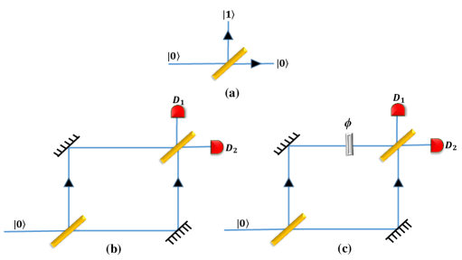
Figure 1: (Color online) A single photon incident at the BS either reflects with certain probability or transmits with the remaining, which provides an optical illustration of qubit in (a). In this case, the outputs travel in perpendicular directions and thus can be interfered at another BS with the help of two mirrors (as shown in (b)), known as MZI. In a standard Mach-Zehnder interferometer with symmetric BSs only one of the detectors clicks, while inserting a phase plate of thickness $t$ in one of the arm (equivalent to applying a phase gate with angle $\phi=\frac{2\pi\left(n-1\right)t}{\lambda}$ with $n$ refractive index of the medium and $\lambda$ wavelength of light used) the clicks on the other detector can be obtained. Here, the BS operation is equivalent to the Hadamard gate.

4 IBM Quantum computer

As we mentioned in the above, qubits can be realized in various ways. In case of the quantum computer placed in cloud by IBM, qubits are realized using Josephson junction. Specifically, the superconducting qubits used in the IBM architecture [1] are known as Transmon qubits.

There are 3 different architectures of computer that are available and can be accessed freely through the internet. The one which was introduced first was known as IBMQX2. Subsequently, two other architectures IBMQX4 and IBMQX5 have been introduced. IBMQX2 and IBMQX4 are 5 qubit quantum computers, whereas IBMQX5 is a 16 qubit quantum computer. In these computers, we are not allowed to implement any arbitrary gate. We have to select gates from a library of gates which is comprised of the gates from Clifford group and $T$ gate. Specifically, it contains three Pauli, identity, Hadamard, phase gates $S\,\left(S^{\dagger}\right)$ and $T\,\left(T^{\dagger}\right)$ as single qubit gates and ${\rm CNOT}$ as 2-qubit gate. It also allows single qubit operations $U1=P\left(\phi\right)$, $U2=\frac{1}{\sqrt{2}}\left[\begin{array}[]{cc}1&-\exp(i\phi)\\ \exp(i\Phi)&\exp(i\phi+i\Phi)\end{array}\right]$, and $U3=\left[\begin{array}[]{cc}\cos\frac{\theta}{2},-\exp(i\phi)\sin\frac{\theta}{2}\\ \exp(i\Phi)\sin\frac{\theta}{2},\exp(i\phi+i\Phi)\cos\frac{\theta}{2}\end{array}\right]$. One can apply single qubit gates at any desired point in the quantum circuits to be built using IBM quantum experience. However, the application of CNOT gate (i.e., the positions in the quantum circuit, where CNOT gate can be applied) is restricted. To be precise, in Fig. 2, we can see that there are certain arrows and the position and direction of the arrows distinguish IBMQX2 and IBMQX4. A particular arrow indicates that a CNOT gate can be applied using the qubit shown at the tail of the arrow as the control qubit and the qubit shown at the head of the arrow as the target qubit. A CNOT is allowed with control on Q0 (Q2) and target on Q2 (Q0) in IBMQX2 (IBMQX4), but the same is not allowed in IBMQX4 (IBMQX2). Actually, the interaction between the qubits are not the same for all choices of two qubits. In fact, the interaction between the qubits is stronger when a qubit having higher frequency is selected as the control qubit, and qubit having lower frequency is chosen to be the target. Thus, the frequencies of the qubits determines the directions in which CNOT gates can be applied directly. In other words, these frequencies lead to the arrows shown in Fig. 2 and thus the architecture of a particular implementation of IBM quantum computer. This map (the architectures shown in Fig. 2) can be written in a compact form. For example, for the IBMQX2 the connectivity map is given by coupling_map = {0: [1, 2], 1: [2], 3: [2, 4], 4: [2]}, where a: [b] means a CNOT with qubit a as control qubit and b as target qubit can be implemented. See that this map describes the architectures shown in Fig. 2 (b). Similarly, the map for IBMQX4 is coupling_map = {1: [0], 2: [0, 1, 4], 3: [2, 4]}. From these coupling maps also (or equivalently from the architectures shown in Fig. 2 (b) and (d)), one can easily recognize that application of CNOT from Q0 to Q2 (Q2 to Q0) is allowed in IBMQX2 (IBMQX4), but is not allowed in IBMQX4 (IBMQX2).

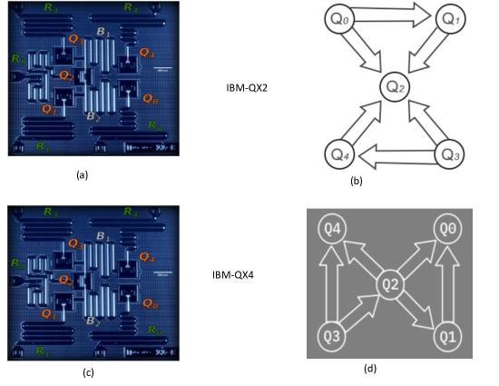
Figure 2: (Color online) Two different architectures of five qubit IBM quantum experience. The difference can be seen from the allowed directions of CNOT. For instance, a CNOT is allowed with control on Q0 (Q2) and target on Q2 (Q0) in IBM-QX2 (IBM-QX4), respectively.

Being superconductivity-based quantum computers, all of these IBMQX* work in very low temperature. Specifically, operating temperature for IBMQX2 and IBMQX4 are 0.0178 K and 0.021K, respectively.

4.1 How to use IBM quantum computer

To start using the IBM quantum computer, you have to first register yourself and thus create a login and password. To do the same please follow the following steps:

1. Open the website of IBM Q Experience, i.e., open https://quantumexperience.ng.bluemix.net/qx/experience [2].

2. Depending on the web-browser used by you either a “Sign in” popup window will open automatically, or you have click on the “Sign in” button on the top right corner which will open a new tab. Subsequently, first time users have to click on “Sign up” button.

3. An account will be created after filling all the required fields.

In this process, your email-id will be your login id and the password is of your choice. Alternatively, one can also login using one of his/her ids of Linkedin, Github, Twitter, etc. After performing registration go to the website [2] and sign in with your credentials. At the top-right corner you will see your name as entered during the registration process. Once you sign in, follow the follwing steps.

1. Click on the “Composer” tab and select a topology that you wish to use for your experiment.
   Note: After clicking on the “Composer” tab, you will be prompted to choose among three available topologies of the IBM quantum computers, namely IBMQX4, IBMQX2, and Custom topology. To run your results on a real quantum computer choose either IBMQX4 or IBMQX2, while Custom topology is useful for running simulation of your circuits. Infact, clicking on the Composer tab (marked at the top in Fig. 3), you will see a window as shown in Fig. 3. You can see that the user name is appearing in the top right. It’s “mitali” in our example. In your case, it will be replaced by your name.
   

2. Select appropriate gates and create your quantum circuit.
   Note: In the lower side of Fig. 3 (i.e., in the lower portion of the window that you have opened in the previous step), you can see five horizontal lines (indexed by ${\rm q[0],\,q[1],\,q[2],\,q[3]}$and ${\rm q[4],}$respectively) representing five qubit lines, on which different unitary operations (quantum gates) allowed in IBM quantum computer can be dropped/dragged after selecting them from the set of gates shown in the right hand side of the qubit lines (see right side of the window/figure). The last line (i.e., the line at the bottom which is indexed by ${\rm c_{0}}$) corresponds to the classical registrar which would store the classical values of the measurement outcomes. In the figure as well as in the window you that you have opened in IBM quantum experience, you can see that all the 5 qubits are initially prepared in the state $|0\rangle.$ Thus, the initial state of an IBM quantum computer is always $|00000\rangle$. Further, you can see that the choice of topology you have made in the previous step is clearly mentioned over the qubit lines as Backend, where units assigned to a user for using the quantum computer are also mentioned. In its left, one can see text “Switch to QASM Editor”, which allows one to design the quantum circuit by writing a program in QASM. We will briefly discuss it in the forthcoming section.

3. Either run or simulate the circuit that you have designed in the previous step. To do so, click on the corresponding tabs (i.e., click either on “Run” tab or on “Simulate” tab).
   Note: To run or simulate the circuit and to see its outcome you have to perform measurement on the appropriate qubits. Once you have designed a circuit and performed measurements on suitable qubits, you will receive your measurement outcomes in the computational basis, i.e., $\left\{|0\rangle,|1\rangle\right\}$. As mentioned above, you can either choose to simulate the output of the circuit or run it on the quantum computer. Next to “Run” and “Simulate” tabs, there are tabs which can be used to change the number of shots you wish to run to obtain the probability distribution of the output. The higher the number of shots the more units are required to run the IBM quantum computer. However, with increase in the number of shots we obtain better results. This point will be established in the next section with the help of an example.

4. In the previous step, the experiment will be performed and you will obtain the result either immediately in a new window (for simulation, we will always obtain it immediately) or the job will be placed in queue and you will receive an email from IBM when the job is executed. Subsequently, you can login again and see the result of your experiment.

In case of difficulty, one can also refer the IBM tutorials available for beginners [8].

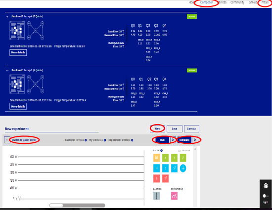
Figure 3: (Color online) The window that we see after clicking the “Composer” tab, where different quantum circuits can be built using drag and drop.

5 Performing simple experiments with IBM quantum computer to clarify the concept of quantum mechanics

5.1 Experiment 1: Is quantum mechanics probabilistic?

We have already introduced the idea of quantum computation and tools that we are going to use to perform our experiments. To begin with, we will try to develop a feeling about the probabilistic nature of quantum mechanics. For this purpose, we may aim to prepare a quantum state $|\psi\rangle=\frac{1}{\sqrt{2}}\left(|0\rangle+|1\rangle\right)$ which is in equal superposition of bit values 0 and 1. In the above we have seen that this state can be obtained as the output of a beam splitter with single photon input (cf. Fig. 1 (a)). In case of IBM quantum computers, the equivalent system can be designed by placing a Hadamard gate in any qubit line. As the Hadamard maps $|0\rangle$ to $\frac{1}{\sqrt{2}}\left(|0\rangle+|1\rangle\right),$ and as the default initial (input) state for each qubit line is $|0\rangle$ in the IBM quantum computers, the output of the Hadamard gate will be in the state $|\psi\rangle=\frac{1}{\sqrt{2}}\left(|0\rangle+|1\rangle\right)$. Now, we perform measurement, choosing number of shots to be 1 (which implies that the measurement is performed only once, i.e., the experiment is not repeated). How many times, you wish to perform the same experiment (repeat the experiment) can be chosen by clicking on the button in the right side of Run button and subsequently clicking on Edit parameters). The single shot measurement would correspond to the situation where a single quantum state $\frac{1}{\sqrt{2}}\left(|0\rangle+|1\rangle\right)$ is measured in the computational basis (circuit is shown in Fig. 4 (a)). Interestingly, in a single run, one can either obtain measurement outcome $|0\rangle$ or $|1\rangle$ as we have shown in Fig. 4 (b) and Fig. 4 (c) which are obtained as outcomes in different runs. Here it’s important to note that the measurement outcome of the IBM quantum computers are to be read from the right to left. The right most bit value corresponds to the outcome of measurement on q[0], next one in the left corresponds to the measurement on q[1], and so on. For example, the outcome of the measurement performed in the circuit shown in Fig. 4 (a) is shown in Fig. 4 (c) as a single bar at 00001. The last digit shows that the measuring q[0] we have obtained 1. As neither any operation nor any measurement is performed on the other qubits output state for them is shown as 0. If we keep on repeating this single shot experiments, we will obtain a random sequence of 0 and 1. This is what happens in the quantum random number generators. Repeated execution of such single shot experiment would convince you that on measurement the wave function (or the state $|\psi\rangle$) randomly collapses to one of the allowed states (in this case either in $|0\rangle$ or in $|1\rangle$). Thus, we have demonstrated the phenomenon of wave function collapse on measurement which is a distinguishing feature of quantum mechanics.

After showing collapse of wavefunction on measurement, we may perform the experiment again with higher numbers of shots, and in Fig. 4 (d)-(f), one can observe that for higher values of shots we have obtained probability distribution of the measurement outcomes. We have already discussed how to select number of shots. If we choose 8192 shots, the experiment will be repeated 8192 times, and in the result probability of obtaining 0 and 1 will be shown. See with the increase in the number of shots i.e., number of times an experiment is repeated, we approach closer to verify the statement that on measurement (in computational basis) a quantum state $|\psi\rangle=\alpha|0\rangle+\beta|1\rangle$ collapses to state $|0\rangle$ and $|1\rangle$ with probabilities $|\alpha|^{2}$ and $|\beta|^{2},$ respectively. In the particular case for which experiment is performed here, we have $\alpha=\beta=\frac{1}{\sqrt{2}}$, and consequently corresponding probabilities are $\frac{1}{2}$ in the ideal situation. In reality, we observe that unless the experiment is repeated a large number of times, the probabilities would not approach $\frac{1}{2}$ (that’s natural in any statistical event). In other words, this shows the statistical nature of quantum mechanics. Further, even for 8192 shots, the probabilities are not exactly $\frac{1}{2}$. This is so partially because of two reasons, (i) even 8192 is not a statistically large number, and (ii) there may be some errors which can be attributed to noise in the quantum system or gate errors.

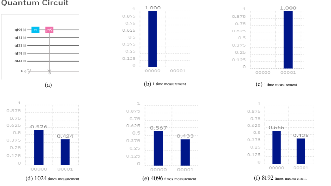
Figure 4: (Color online) Randomness intrinsic in quantum mechanics is shown with the help of measuring an equal superposition state in the computational basis (as shown in (a)) in (b) and (c) for single run. However, probabilistic interpretation that we use requires higher number of runs. With increase in the values of runs we can observe equal probabilities for both measurement outcomes.

5.1.1 Application of Experiment 1: Quantum random number generator

The experiment discussed here not only establishes the probabilistic nature of quantum mechanics, but also forms the basis for generating a string of true random numbers. Note that there does not exist a true random number generator in the domain of classical physics, while due to inherent randomness of quantum mechanics a quantum random number generator can be built. The fact that classical random numbers are not truly random, can be easily visualized through a lucid example. Consider the outputs of repeated tossing of a coin. Usually we would expect the outputs to be random. However, if we know the air drag, weight of the coin, force applied at the time of throwing the coin, height at the time of throwing, gravitational acceleration, etc., we can in principle solve the equation of motion and predict the output. So the output is not random. Here, randomness actually arises due to our ignorance. In contrast, quantum mechanics is intrinsically probabilistic.

The working of an easily available quantum random number generator involves simple optical elements- a symmetric BS and two detectors. Specifically, performing measurement in the two output ports of the BS in Fig. 1 (a) one can obtain a string of 0s and 1s. Corresponding experiment performed on IBM quantum experience with shot value 1 as shown in Fig. 4 (a) gives random outputs 0 and 1 as in Fig. 4 (b) and (c), respectively. A repetitive preparation of this initial state and its measurement in the computational basis can be used to obtain a string of true random numbers. Subsequently, an interested reader can perform various randomness tests to ensure that the generated numbers are random. See [11] for the tools for various types randomness tests recommended by NIST. Here, it may be noted that random number generators are used in some ATMs, Casinos, in Weather predictions, stock-market predictions, etc., and in many other places including state lottery boards. In brief, the simple experiment described above not only illustrates a distinct character of quantum mechanics, it also establishes quantum supremacy in context of a particular application of quantum mechanics that has relevance in our day to day life.

5.2 Experiment 2: Mach-Zehnder interferometer

We have discussed MZI while discussing optical circuits. We have shown that due to insertion of a phase plate (with phase angle $\phi$), the output bit values 0 and 1 are obtained with probabilities $\cos^{2}\frac{\phi}{2}$ and $\sin^{2}\frac{\phi}{2}$, respectively. For our experiments Hadamard gate works like a BS, and consequently applications of 2 consecutive Hadmard gates will be equivalent to a Machzehnder interfeorometer as it would imply the use of output of first BS as the input of second BS. The role of mirrors in the original MZI is just to redirect the output of the first BS to the input ports of the second BS, so in IBM quantum computer, we don’t need any component (gate) analogous to mirror. Now, a Mach-Zehnder interferometer with a phase plate in one of the path (as shown in Fig. 1) should be equivalent to a circuit in which a phase gate is inserted between two Hadamards. Such a circuit designed for the implementation in IBM quantum computer is shown in the top-left corner in Fig. 5. We performed the experiment using this circuit in IBM quantum computer with different values of $\phi$ and prepared a table of values of probability of measurement outcome 0. Some of the obtained results are also shown Fig. 5 for illustration. We obtained the variation of probability of detector click (correspond to bit value 0) and have shown it to fit with the plot of $\cos^{2}\frac{\phi}{2}$ (cf. Fig. 6). Thus, our experimental results match exactly with the theoretically calculated value.

Here it is important to note that the first experiment performed here (which led to random number generator) does not establish the the fact that a quantum state simultaneously existed in state $|0\rangle$ and $|1\rangle$sates. Consider a model which tells that a quantum particle after interacting with the BS randomly goes to the reflected path in 50% cases and in the transmitted cases in the rest of the cases. In that case also the detectors placed after the BS (see Fig. 1) would have clicked randomly. So the previous experiment cannot distinguish between this theory and the theory that tells that a quantum state simultaneously remains in $|0\rangle$ and $|1\rangle.$ However, as soon as we add the next BS in the MZI, this theory would imply that independent of the fact whether the quantum particles come from the reflected path or the transmitted path, half of them will go to one detector after the second BS and rest will go to the second detector. However, if the interpretation of quantum mechanics which states that the quantum particle simultaneously stays in both the paths is correct then constructive interference will happen in one of the detectors (which will always click) and destructive interference will happen on the other detector (which will never click). Applying two consecutive Hadamards in IBM, we can demonstrate that the quantum states really stay in the superposition state and the crude model described in this paragraph is wrong.

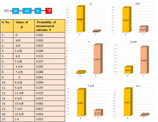
Figure 5: (Color online) MZI realized in IBM quantum experience. Probabilities of obtaining measurement outcome 0 for different values of the phase angle $\phi$ are summarized in table. Few particular cases (for specific values of $\phi$) as output of IBM quantum experience are also shown.

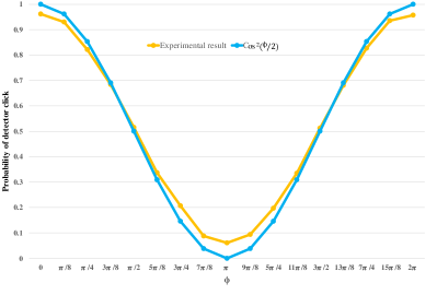
Figure 6: (Color online) The experimental output of MZI (realized using IBM quantum computer) is shown to fit nicely with the corresponding theoretical results.

5.2.1 Application of Experiment 2: Interaction free measurement and quantum cryptography

In this experiment, we have seen that MZI can be implemented using IBM quantum computer. It’s interesting for various reasons. Specifically, MZI and its variants have been used to realize numerous quantum communication and computation schemes. For instance, Goldenberg-Vaidman [3] and Guo-Shi [4] protocols of quantum key distribution essentially use MZI (see Chapter 8 of Ref. [5] for details). Further, counterfactual quantum communication proposed in the recent past [6] and experimentally performed recently [7] employ chained MZI.

5.3 Experiment 3: Prepare and visualize an entangled state

Suppose that there are two quantum systems indexed by the subscripts $A$ and $B$ and they form a composite system indexed by subscript $AB$. Thus, the systems indexed by the subscripts $A$ and $B$ can be considered as the subsystems of a bigger (composite) system indexed by subscript $AB$. Further, consider that the quantum state of the first subsystem is $|\psi\rangle_{A}$ and that of the second subsystem is $|\psi\rangle_{B}$. Now, if we can write $|\psi\rangle_{AB}=|\psi\rangle_{A}|\psi\rangle_{B}$ then the composite state is called separable and otherwise it’s called entangled or inseparable. For a better understanding of entanglement one has to read about tensor product (see Chapter 3 of [9]). However, it’s possible to develop a feeling of entangled state through some simple examples. To provide a lucid idea, let us think that the subsystems $A$ and $B$ are single qubit systems. Now if we have $|\psi\rangle_{AB}=\frac{1}{\sqrt{2}}\left(|00\rangle+|10\rangle\right)_{AB}$, we can easily see that the second qubit is always in the state $|0\rangle$ and $|\psi\rangle_{AB}$ can be separated (factorized in a lucid sense) in the form $|\psi\rangle_{AB}=|\psi\rangle_{A}|\psi\rangle_{B}$ as follows $|\psi\rangle_{AB}=\frac{1}{\sqrt{2}}\left(|00\rangle+|10\rangle\right)_{AB}=\frac{1}{\sqrt{2}}\left(|0\rangle+|1\rangle\right)_{A}|\psi\rangle_{B}$. Thus, the state $|\psi\rangle_{AB}=\frac{1}{\sqrt{2}}\left(|00\rangle+|10\rangle\right)_{AB}$ is separable (as you can separate the states of the first and second qubits). Now, you can see that following sates are not separable in the above sense: $|\psi^{+}\rangle_{AB}=\frac{1}{\sqrt{2}}\left(|00\rangle+|11\rangle\right)_{AB}$ and $|\phi^{+}\rangle_{AB}=\frac{1}{\sqrt{2}}\left(|01\rangle+|10\rangle\right)_{AB}$. Being inseparable, these states are called entangled. These states have no classical analogue and the collapse on measurement described and verified earlier leads to very interesting consequences for these states. To begin with you can see that if you measure the first qubit in the state $|\psi^{+}\rangle_{AB}=\frac{1}{\sqrt{2}}\left(|00\rangle+|11\rangle\right)_{AB}$ and obtain $|0\rangle_{A}$ then the other qubit must collapse to $|0\rangle_{B}$. Similarly, if your measurement on the first qubit yields $|1\rangle_{A}$ then the state of the second qubit must become $|1\rangle_{B}$ . Thus, there is a kind of quantum correlation. Let us now show you how to produce $|\psi^{+}\rangle$ and $|\phi^{+}\rangle$in IBM quantum computer and what kind of outcome is obtained in the measurement. However, for the completeness of the article, instead of using the drag and draw approach, here we will follow another method for preparing the quantum circuits. To be precise, as mentioned above, after opening composure we have clicked on the "Switch to QASM Editor" tab and that has led us to a black window, where we have written a simple QASM code (see left panel of Fig. 7 (a) to generate the quantum circuit shown in Fig. 7 (b) which would produce a two-qubit entangled state $|\psi^{+}\rangle$). On measurement, the output of this circuit is expected to be 00 or 11, so we can expect two bars of equal or almost equal height one at 00000 and one at 00011. However, by performing the real experiment, we found the output shown in Fig. 7 (b), where we can see a small but finite probability of obtaining 00001 and 00010, too. These, two small bars appears as a manifestation of gate errors and channel noise. Once, you see that even for a small circuit with only 2 gates, noise can affect the output to some extent, you can easily recognize what restricts us from building large (scalable) quantum computers. Finally, in Fig. 7 (c), we show a circuit that would produce the entangled state $|\phi^{+}\rangle$.

We would like to suggest the young readers to replace Hadamard gate with U3 gate in the circuits shown in Fig. 7 (a) and (c), and to obtain the corresponding results in the tabular form as was shown in Fig. 5. This exercise, would help them to understand the idea of maximally and non-maximally entangled states.

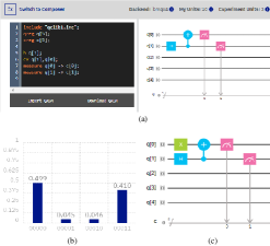
Figure 7: (Color online) In addition to drag and drop approach, one can also use QASM to write the circuits. Here, as an example, we have shown generation of entanglement using a Hadamard and a CNOT gate.

5.3.1 Applications of Experiment 3: Quantum key distribution, entanglement swapping and quantum repeaters

As mentioned previously, that the measurement outcomes of the entangled state $\frac{1}{\sqrt{2}}\left(|00\rangle+|11\rangle\right)$ in the computational basis are symmetric, two distant parties sharing multiple copies of this state can form a symmetric string of random numbers to be used as unconditionally secure quantum key. Starting with two copies of the entangled state and measuring both the first qubits in the Bell basis, the last two qubits get entangled. This is termed as entanglement swapping. The idea of entanglement swapping is useful in long distance quantum communication where entanglement between two distant parties can be shared with the help of measurements in Bell basis as quantum repeaters.

Here we have mentioned only a few simple applications of entanglement. Interested readers may read about quantum teleportation, dense coding, remote state preparation, etc., which are more convincing applications of entangled states. To be precise, none of these quantum phenomena can be obtained without the use of quantum entanglement.

6 Conclusion

In the above, we have seen that the nonclassical features of quantum mechanics can be tested through some simple experiments in the class room, and such experimental realizations and their modifications have direct applications in performing tasks having socio-economic relevance. The experiments and applications mentioned here are only the representative cases. Many such experiments can be designed and analyzed. Such experiments can also be used to teach advanced topics of quantum mechanics through the experiments done using IBM quantum computer. Experimental studies also require one to compute fidelity of the quantum states, which can be reconstructed by quantum state tomography (see [10] for detail). We conclude the article with a hope that the interested teachers and students will try to design new experiments with the help of this article and the texts mentioned in the Further reading section, will provide the backbone for such new designs.

Further reading

1. Optical quantum information and quantum communication, A. Pathak and A. Banerjee, SPIE Spotlight Series, SPIE Press (2016) ISBN: 9781510602212

2. Light and its Many Wonders, A. Ghatak, A. Pathak and V. P. Sharma (Eds.), Viva Books, New Delhi, India (2015) ISBN 978-81-309-3428-0

3. Beck, Mark. Quantum mechanics: theory and experiment. Oxford University Press, 2012.

Acknowledgment: AP thanks Defense Research and Development Organization (DRDO), India for the support provided through the project number ERIP/ER/ 1403163 /M/01/ 1603. He also thanks K. Thapliyal and M. Sisodia for their technical feedback and help.

References

- [1] J. M. Gambetta, J. M. Chow and M. Steffen, "Building logical qubits in a superconducting quantum computing system", npj Quantum Information 3, 2 (2017)
- [2] https://quantumexperience.ng.bluemix.net/qx/experience
- [3] Goldenberg L., Vaidman L., “Quantum cryptography based on orthogonal states”, Physical Review Letters, vol. 75, p. 1239, 1995.
- [4] Guo, G.C. and Shi, B.S., Quantum cryptography based on interaction-free measurement. Phys. Lett. A 256, 109–112 (1999)
- [5] Light and its Many Wonders, A. Ghatak, A. Pathak and V. P. Sharma (Eds.), Viva Books, New Delhi, India (2015) ISBN 978-81-309-3428-0
- [6] Salih H., Li Z.H., Al-Amri M., Zubairy M.S., “Protocol for direct counterfactual quantum communication”, Physical Review Letters, vol. 110, p. 170502, 2013.
- [7] Cao Y., Li Y.H., Cao Z., Yin J., Chen Y.A., Yin H.L., Chen T.Y., Ma X., Peng C.Z., Pan J.W., “Direct counterfactual communication via quantum Zeno effect”, Proceedings of the National Academy of Sciences, vol. 114, pp. 4920–4924, 2017.
- [8] https://quantumexperience.ng.bluemix.net/proxy/tutorial/beginners-guide/introduction.html
- [9] Pathak, A.: Elements of Quantum Computation and Quantum Communication. Taylor & Francis (2013)
- [10] Sisodia, Mitali, Abhishek Shukla, Kishore Thapliyal, and Anirban Pathak. "Design and experimental realization of an optimal scheme for teleportation of an -qubit quantum state." Quantum Information Processing 16, no. 12 (2017): 292.
- [11] A Statistical Test Suite for Random and Pseudorandom Number Generators for Cryptographic Applications, National Institute of Standards and Technology (NIST) Special Publication 800-22, Rev. 1a, 2010.