Temperature Dependent Density Profiles of Dipolar Droplets

Abstract

Recently, trapped dipolar gases were observed to form high density droplets in a regime where mean field theory predicts collapse. These droplets present a novel form of equilibrium where quantum fluctuations are critical for stability. So far, the effect of quantum fluctuations have only been considered at zero temperature through the local chemical potential arising from the Lee–Huang–Yang correction. Here, we extend the theory of dipolar droplets to non-zero temperatures using Hartree–Fock–Bogoliubov theory (HFBT), and show that the equilibrium is strongly affected by temperature fluctuations. HFBT, together with local density approximation for excitations, reproduces the zero temperature results, and predict that the condensate density can change dramatically even at low temperatures where the total depletion is small. Particularly, we find that typical experimental temperatures ($T\sim$ 100 nK) can significantly modify the transition between low density and droplet phases.

I Introduction

Experiments on ultracold atoms with dipole-dipole interactions provide opportunities to explore novel physical regimes. So far, Bose-Einstein condensates where dipolar interaction plays a dominant role have been achieved for chromium Griesmaier et al. (2005), dysprosium Lu et al. (2011) and erbium Aikawa et al. (2012). The long range and anisotropic interaction make these systems non–trivial and susceptible to catastrophic collapse Lahaye et al. (2009). Recent experiments have surprisingly found that dipolar gases have a stable droplet phase in a parameter range where mean field theory predicts collapse Kadau et al. (2016); Chomaz et al. (2016).

Formation of stable dipolar droplets were first reported by the Stuttgart group Kadau et al. (2016). Subsequent experiments were able to isolate single droplets Ferrier-Barbut et al. (2016), and show that they can be stable even without external trapping Schmitt et al. (2016). Similarly, the phase transition between trapped cloud and the droplet has been explored for erbium Chomaz et al. (2016).

Mean field theory in the form of Gross–Pitaevskii (GP) approximation have been successfully used to explain the physics of ultracold bosonic systems including dipolar BECs O’Dell et al. (2004). However, GP equation predicts collapse of dipolar BECs in the regime tested by the droplet experiments Santos et al. (2003). Hence, the stability of droplets must either stem from higher order interactions Bisset and Blakie (2015); Xi and Saito (2016), or beyond mean field effects Petrov (2015); Wächtler and Santos (2016). Experiments have clearly demonstrated that beyond mean field effects are better candidates for the stability mechanism Ferrier-Barbut et al. (2016). Quantum fluctuations included as a local Lee-Huang-Yang (LHY) chemical potential correction Lee et al. (1957) has successfully explained experimentally observed phase transition Bisset et al. (2016). Although this energy correction is small compared to the mean field terms, it is crucial for the equilibrium observed in the droplet phase.

While it is intuitively appealing to include the energy cost of quantum fluctuations as a local change in the chemical potential, this approach is not transparent as to which approximations are made in its derivation. There are systematic approximation methods to calculate the effect of quantum fluctuations on mean field equations Griffin (1996). In this paper, we use HFBT to take the feedback effect of fluctuations on the condensate into account. Fluctuations are described by the Bogoliubov–de Gennes (BdG) equations, and we show that solving BdG equations locally reproduces the generalized GP approach used in the current literature Wächtler and Santos (2016); Bisset et al. (2016). The success of this equation to explain the experiments is then seen to be a clear consequence of the depleted density being much lower than the condensate density. We also show that, contrary to a recent claim Boudjemâa (2017), HFBT approach is enough by itself to describe the droplet phase, without the ad-hoc inclusion of the LHY term in the chemical potential.

Generally, the density profile of a BEC depends only weakly on the temperature as long as it is small compared to the transition temperature Giorgini et al. (1996). Even the collective oscillation frequencies of BECs are modified by temperature only if there is a significant thermal component in the cloud Jin et al. (1997). Thus, the density profile of the condensate is generally calculated within the GP approximation without any reference to the temperature. In this paper, we show that this is no longer true for the dipolar clouds close to the droplet transition. When the stability of the system is provided by fluctuations, temperature effects become non negligible. HFBT is easily generalized to non zero temperatures, and clearly shows that the LHY local term can be modified significantly by temperature even if the total depletion remains small.

This paper is organized as follows: We first discuss the HFBT approach starting from the Hamiltonian, and then solve BdG equations within the local density approximation. These approximations yield the generalized GP equation Wächtler and Santos (2016); Bisset et al. (2016) up to a small correction. Subsequently, we discuss the relevant temperature scales in the experiments and calculate how the LHY term depends on the temperature. Finally, we use this theory to investigate the dependence of the density profile on temperature and argue that temperature effects could be relevant in the current experiments.

II Hartree-Fock-Bogoliubov Theory

The Hamiltonian for a trapped dipolar Bose gas is:

$$\hat{H} = \int d^{3}\mathbf{x}\hat{\psi}^{\dagger}(\mathbf{x})h_{0}(\mathbf{x})\hat{\psi}(\mathbf{x})$$

$$+ \frac{1}{2}\iint d^{3}\mathbf{x}d^{3}\mathbf{x}^{\prime}\hat{\psi}^{\dagger}(\mathbf{x})\hat{\psi}^{\dagger}(\mathbf{x}^{\prime})V_{\text{int}}(\mathbf{x}-\mathbf{x}^{\prime})\hat{\psi}(\mathbf{x}^{\prime})\hat{\psi}(\mathbf{x}),$$

where the Bosonic field operators satisfy $[\hat{\psi}(\mathbf{x}),\hat{\psi}^{\dagger}(\mathbf{x}^{\prime})]=\delta(\mathbf{x}-\mathbf{x}^{\prime})$. Single particle Hamiltonian $h_{0}(\mathbf{x})=-\frac{\hbar^{2}\nabla^{2}}{2M}+U_{\text{tr}}(\mathbf{x})-\mu$, contains the kinetic energy, trapping potential $U_{\text{tr}}(\mathbf{x})$ and the chemical potential $\mu$. The particles interact through short range repulsion $g=4\pi\hbar^{2}a_{s}/M$ and long range dipolar potential, $V_{\text{int}}(\mathbf{x})=g\left[\delta(\mathbf{x})+\frac{3\epsilon_{dd}}{4\pi|\mathbf{x}|^{3}}\left(1-3\frac{z^{2}}{|\mathbf{x}|^{2}}\right)\right]$, where $\epsilon_{dd}=C_{dd}/3g$ is the dimensionless dipole interaction strength expressed in terms of s-wave scattering length $a_{s}$.

In the existence of a macroscopically occupied condensate state ($N-N_{0}\ll N$, where $N$ is the total number of atoms, and $N_{0}$ is the number of condensate atoms), the field operator can be approximated by a classical mean field plus fluctuations: $\hat{\psi}(\textbf{x})=\Psi(\textbf{x})+\hat{\phi}(\textbf{x})$. These fluctuation operators, $\hat{\phi}$, satisfy the commutation relations, $\left[\hat{\phi}(\textbf{x}),\hat{\phi}^{\dagger}(\textbf{x}^{\prime})\right]=\delta(\textbf{x}-\textbf{x}^{\prime})-\Psi(\textbf{x})\Psi^{*}(\textbf{x}^{\prime})/N_{0}$ and $\left[\hat{\phi}(\textbf{x}),\hat{\phi}(\textbf{x}^{\prime})\right]=\left[\hat{\phi}^{\dagger}(\textbf{x}),\hat{\phi}^{\dagger}(\textbf{x}^{\prime})\right]=0$. Then, the non-condensate densities, direct and anomalous, are given by $\tilde{n}(\textbf{x}^{\prime},\textbf{x})=\langle\hat{\phi}^{\dagger}(\textbf{x}^{\prime})\hat{\phi}(\textbf{x})\rangle$ $(\tilde{n}(\textbf{x})=\langle\hat{\phi}^{\dagger}(\textbf{x})\hat{\phi}(\textbf{x})\rangle)$, and $\tilde{m}(\textbf{x}^{\prime},\textbf{x})=\langle\hat{\phi}(\textbf{x}^{\prime})\hat{\phi}(\textbf{x})\rangle$. As our focus is the stabilization of the condensate due to fluctuations, we will not perturbatively expand in the fluctuation operators, but consider their feedback on the condensate Griffin (1996). Hartree-Fock-Bogoliubov theory includes third and higher order terms via Hartree-Fock factorization Griffin (1996). When applied to third order terms in the Hamiltonian, this factorization generates:

$$\hat{\phi}^{\dagger}(\textbf{x})\hat{\phi}^{\dagger}(\textbf{x}^{\prime})\hat{\phi}(\textbf{x}^{\prime}) \approx\tilde{m}^{*}(\textbf{x}^{\prime},\textbf{x})\hat{\phi}(\textbf{x}^{\prime})+\tilde{n}^{*}(\textbf{x}^{\prime},\textbf{x})\hat{\phi}^{\dagger}(\textbf{x}^{\prime})+\tilde{n}(\textbf{x}^{\prime})\hat{\phi}^{\dagger}(\textbf{x})$$

$$\hat{\phi}^{\dagger}(\textbf{x})\hat{\phi}(\textbf{x}^{\prime})\hat{\phi}(\textbf{x}) \approx\tilde{n}^{*}(\textbf{x}^{\prime},\textbf{x})\hat{\phi}(\textbf{x})+\tilde{n}(\textbf{x})\hat{\phi}(\textbf{x}^{\prime})+\tilde{m}(\textbf{x}^{\prime},\textbf{x})\hat{\phi}^{\dagger}(\textbf{x})$$

$$\hat{\phi}^{\dagger}(\textbf{x})\hat{\phi}^{\dagger}(\textbf{x}^{\prime})\hat{\phi}(\textbf{x}) \approx\tilde{m}^{*}(\textbf{x}^{\prime},\textbf{x})\hat{\phi}(\textbf{x})+\tilde{n}(\textbf{x})\hat{\phi}^{\dagger}(\textbf{x}^{\prime})+\tilde{n}(\textbf{x}^{\prime},\textbf{x})\hat{\phi}^{\dagger}(\textbf{x})$$

$$\hat{\phi}^{\dagger}(\textbf{x}^{\prime})\hat{\phi}(\textbf{x}^{\prime})\hat{\phi}(\textbf{x}) \approx\tilde{n}(\textbf{x}^{\prime})\hat{\phi}(\textbf{x})+\tilde{n}(\textbf{x}^{\prime},\textbf{x})\hat{\phi}(\textbf{x}^{\prime})+\tilde{m}(\textbf{x}^{\prime},\textbf{x})\hat{\phi}^{\dagger}(\textbf{x}^{\prime}).$$ (2)

The Hamiltonian, then, consists of terms of zeroth, first and second order in fluctuations. In the many particle ground state the first order terms in fluctuations must vanish. Therefore, the condensate wavefunction must obey the Gross-Pitaevskii equation:

$$\mathcal{L}\Psi(\textbf{x})+\int d^{3}\textbf{x}^{\prime}V_{\text{int}}(\textbf{x}-\textbf{x}^{\prime})\tilde{n}(\textbf{x}^{\prime},\textbf{x})\Psi(\textbf{x}^{\prime})+\int d^{3}\textbf{x}^{\prime}V_{\text{int}}(\textbf{x}-\textbf{x}^{\prime})\tilde{m}(\textbf{x}^{\prime},\textbf{x})\Psi^{*}(\textbf{x}^{\prime})=0,$$ (3)

where $\mathcal{L}=\left[-\hbar^{2}\nabla^{2}/2M-\mu+U_{\text{tr}}(\textbf{x})+\int d^{3}\textbf{x}^{\prime}V_{\text{int}}(\textbf{x}-\textbf{x}^{\prime})|\Psi(\textbf{x}^{\prime})|^{2}+\int d^{3}\textbf{x}^{\prime}V_{\text{int}}(\textbf{x}-\textbf{x}^{\prime})\tilde{n}(\textbf{x}^{\prime})\right],$ includes not only the single particle Hamiltonian, but also the Hartree potential $\Phi_{H}(\mathbf{x})=\int d^{3}\mathbf{x}^{\prime}V_{\text{int}}(\mathbf{x}-\mathbf{x}^{\prime})(|\Psi(\mathbf{x}^{\prime})|^{2}+\tilde{n}(\mathbf{x}^{\prime}))$. Fluctuation terms generate the direct non-condensate density $\tilde{n}(\mathbf{x}^{\prime},\mathbf{x})=\langle\hat{\phi}^{\dagger}(\mathbf{x}^{\prime})\hat{\phi}(\mathbf{x})\rangle$, and the anomalous non-condensate density $\tilde{m}(\mathbf{x}^{\prime},\mathbf{x})=\langle\hat{\phi}(\mathbf{x}^{\prime})\hat{\phi}(\mathbf{x})\rangle$.

Excitation modes and energies are found via the diagonalization of the Hamiltonian. Although the fourth order terms in the Hamiltonian can be reduced to second order ones via the Hartree–Fock factorization, we neglect these terms since they solely involve the interaction among the depleted particles. Such terms are important only if the depleted density is comparable to the condensate density. The Hamiltonian is diagonal in the quasiparticle excitations given by the Bogoliubov transformation:

$$\hat{\phi}(\textbf{x}) =\sum_{j}u_{j}(\textbf{x})\hat{\alpha}_{j}-v^{*}_{j}(\textbf{x})\hat{\alpha}^{\dagger}_{j}$$

$$\hat{\phi}^{\dagger}(\textbf{x}) =\sum_{j}u^{*}_{j}(\textbf{x})\hat{\alpha}^{\dagger}_{j}-v_{j}(\textbf{x})\hat{\alpha}_{j},$$ (4)

where, $\hat{\alpha}$ are the quasiparticle operators satisfying $\left[\hat{\alpha}_{j},\hat{\alpha}^{\dagger}_{k}\right]=\delta_{j,k}$ and $\left[\hat{\alpha}_{j},\hat{\alpha}_{k}\right]=\left[\hat{\alpha}^{\dagger}_{j},\hat{\alpha}^{\dagger}_{k}\right]=0$. This transformation yields the Bogoliubov-de Gennes equations:

$$\mathcal{L}_{0}u_{j}(\textbf{x})+\int d^{3}\textbf{x}^{\prime}V_{\text{int}}(\textbf{x}-\textbf{x}^{\prime})\Psi^{*}(\textbf{x}^{\prime})\Psi(\textbf{x})u_{j}(\textbf{x}^{\prime})-\int d^{3}\textbf{x}^{\prime}V_{\text{int}}(\textbf{x}-\textbf{x}^{\prime})\Psi(\textbf{x}^{\prime})\Psi(\textbf{x})v_{j}(\textbf{x}^{\prime})=E_{j}u_{j}(\textbf{x})$$ (5)

$$\mathcal{L}_{0}v_{j}(\textbf{x})+\int d^{3}\textbf{x}^{\prime}V_{\text{int}}(\textbf{x}-\textbf{x}^{\prime})\Psi(\textbf{x}^{\prime})\Psi^{*}(\textbf{x})v_{j}(\textbf{x}^{\prime})-\int d^{3}\textbf{x}^{\prime}V_{\text{int}}(\textbf{x}-\textbf{x}^{\prime})\Psi^{*}(\textbf{x}^{\prime})\Psi^{*}(\textbf{x})u_{j}(\textbf{x}^{\prime})=-E_{j}v_{j}(\textbf{x}),$$ (6)

where $\mathcal{L}_{0}=\left[-\hbar^{2}\nabla^{2}/2M-\mu+U_{\text{tr}}(\textbf{x})+\int d^{3}\textbf{x}^{\prime}V_{\text{int}}(\textbf{x}-\textbf{x}^{\prime})|\Psi(\textbf{x}^{\prime})|^{2}\right].$ Bogoliubov amplitudes further satisfy,
$\int d^{3}\textbf{x}\left[u_{j}^{*}(\textbf{x})u_{k}(\textbf{x})-v^{*}_{j}(\textbf{x})v_{k}(\textbf{x})\right]=\delta_{j,k}$, and $\int d^{3}\textbf{x}\left[u_{j}(\textbf{x})v_{k}(\textbf{x})-u_{k}(\textbf{x})v_{j}(\textbf{x})\right]=0$.

Since the excitation modes are decoupled, the following expectation values are given by Bose statistics,

$$\left\langle\hat{\alpha}^{\dagger}_{j}\hat{\alpha}_{k}\right\rangle = \delta_{j,k}N_{B}(E_{j})$$

$$\left\langle\hat{\alpha}_{j}\hat{\alpha}_{k}\right\rangle = \left\langle\hat{\alpha}^{\dagger}_{j}\hat{\alpha}^{\dagger}_{k}\right\rangle=0,$$ (7)

where $N_{B}(E)=1\left/\left(\exp\left[\frac{E}{k_{B}T}\right]-1\right)\right.$. This yields temperature dependent depletion density expressions:

$$\tilde{n}(\textbf{x}^{\prime},\textbf{x})=\sum_{j}\left(v_{j}(\textbf{x}^{\prime})v_{j}^{*}(\textbf{x})+N_{B}(E_{j})\left[u_{j}^{*}(\textbf{x}^{\prime})u_{j}(\textbf{x})+v_{j}(\textbf{x}^{\prime})v_{j}^{*}(\textbf{x})\right]\right)$$ (8)

$$\tilde{m}(\textbf{x}^{\prime},\textbf{x})=-\sum_{j}\left(u_{j}(\textbf{x}^{\prime})v_{j}^{*}(\textbf{x})+N_{B}(E_{j})\left[v_{j}^{*}(\textbf{x}^{\prime})u_{j}(\textbf{x})+u_{j}(\textbf{x}^{\prime})v_{j}^{*}(\textbf{x})\right]\right).$$ (9)

In principle, a numerical solution of the above set would determine both the condensate density and the excitation frequencies. However, such a determination of stability is computationally expensive, and numerical approaches so far required further approximations. For example in Ronen and Bohn (2007) the normal density matrix is assumed to be diagonal real space $\tilde{n}(\textbf{x}^{\prime},\textbf{x})\propto\delta(\textbf{x}^{\prime},\textbf{x})$, which misses most of the dipolar contribution to the local LHY potential. This approximation is repeated in Boudjemâa (2017), and the LHY term is added separately to the BdG equation. Simpler approaches based on the generalized GP provide more insight as well as quantitative predictions in line with the droplet experiments Wächtler and Santos (2016); Bisset et al. (2016); Chomaz et al. (2016). HFB theory introduces three new terms into the GP equation: the direct interaction between condensed atoms and depleted atoms,

$$\Phi_{H}^{(1)}(\textbf{x})=\int d^{3}\textbf{x}^{\prime}V_{\text{int}}(\textbf{x}-\textbf{x}^{\prime})\tilde{n}(\textbf{x}^{\prime}),$$ (10)

and the fluctuation terms,

$$\Omega^{(n)}(\textbf{x})\Psi(\textbf{x}) =\int d^{3}\textbf{x}^{\prime}V_{\text{int}}(\textbf{x}-\textbf{x}^{\prime})\tilde{n}(\textbf{x}^{\prime},\textbf{x})\Psi(\textbf{x}^{\prime})$$ (11)

$$\Omega^{(m)}(\textbf{x})\Psi(\textbf{x}) =\int d^{3}\textbf{x}^{\prime}V_{\text{int}}(\textbf{x}-\textbf{x}^{\prime})\tilde{m}(\textbf{x}^{\prime},\textbf{x})\Psi^{*}(\textbf{x}^{\prime}).$$ (12)

These fluctuations can be interpreted as local corrections for the chemical potential $\Delta\mu(\textbf{x})=\Omega^{(n)}(\textbf{x})+\Omega^{(m)}(\textbf{x})$. Therefore, the generalized GP equation becomes:

$$\Big{[}-\frac{\hbar^{2}\nabla^{2}}{2M}-\mu+U_{\text{tr}}(\textbf{x})+\Phi_{H}(\textbf{x})+\Delta\mu(\textbf{x})\Big{]}\Psi(\textbf{x})=0,$$ (13)

where $\Phi_{H}(\textbf{x})=\int d^{3}\textbf{x}^{\prime}V_{\text{int}}(\textbf{x}-\textbf{x}^{\prime})\left(|\Psi(\textbf{x}^{\prime})|^{2}+\tilde{n}(\textbf{x}^{\prime})\right).$ In the next section we show that the local evaluation of these terms result in the generalized GP equation used in the literature without any further assumptions. HFBT combined with local density approximation for fluctuations results in the generalized GP equation directly, no ad-hoc terms are needed for the description of the stable droplet.

III Local Density Approximation

In this section, we give two results which arise when the local density approximation is applied to the HFBT theory given in the previous section. First, when LDA is applied to BdG equations fluctuation modes can be analytically obtained which reduce the GP equation to the modified GP currently used in the literature to describe the droplets. The second result is that this analysis, including the LDA, can be straightforwardly generalized to non-zero temperatures.

If the condensate density and the trapping potential vary slowly on the scale of the wavelength of the BdG modes, Eqs.5,6 can be solved with a local density approximation Lima and Pelster (2012) in the spirit of the semi-classical WKB approximation. This approximation gets more accurate for higher energy modes which makes it more suitable for finite size systems like droplets.

Under the assumption that the condensate density is a slowly varying function of position, one substitutes Lima and Pelster (2012)

$$u_{j}(\textbf{x})\rightarrow u(\textbf{x},\textbf{k})e^{i\textbf{k}\cdot\textbf{x}}\qquad E_{j}\rightarrow E(\textbf{x},\textbf{k})\qquad\sum_{j}\rightarrow\int\frac{d^{3}\textbf{k}}{(2\pi)^{3}},$$ (14)

where $u(\textbf{x},\textbf{k})$ is also a slowly varying function of position. The orthogonality condition for the excitation amplitudes then reads $|u(\textbf{x},\textbf{k})|^{2}-|v(\textbf{x},\textbf{k})|^{2}=1$. The fluctuation terms can be expressed within the same LDA as

$$\Omega_{n}(\textbf{x})=\int\frac{d^{3}\textbf{k}}{(2\pi)^{3}}\tilde{V}_{\text{int}}(\textbf{k})\left(|v(\textbf{x},\textbf{k})|^{2}+N_{B}(E(\textbf{x},\textbf{k}))\left[|u(\textbf{x},\textbf{k})|^{2}+|v(\textbf{x},\textbf{k})|^{2}\right]\right)$$ (15)

$$\Omega_{m}(\textbf{x})=\int\frac{d^{3}\textbf{k}}{(2\pi)^{3}}\tilde{V}_{\text{int}}(\textbf{k})\left(-u(\textbf{x},\textbf{k})v^{*}(\textbf{x},\textbf{k})-2N_{B}(E(\textbf{x},\textbf{k}))u(\textbf{x},\textbf{k})v^{*}(\textbf{x},\textbf{k})\right),$$ (16)

where $\tilde{V}_{\text{int}}(\textbf{k})=g[1+\epsilon_{dd}(3\cos^{2}\theta_{\textbf{k}}-1)]$ is the Fourier transform of the interaction potential. Using, $e^{-i\textbf{k}\cdot\textbf{x}}\mathcal{L}u(\textbf{x},\textbf{k})e^{i\textbf{k}\cdot\textbf{x}}\approx\varepsilon_{\textbf{k}}u(\textbf{x},\textbf{k})$, and

$$\Psi(\textbf{x})\int d^{3}\textbf{x}^{\prime}V_{\text{int}}(\textbf{x}-\textbf{x}^{\prime})\Psi(\textbf{x}^{\prime})u(\textbf{x}^{\prime},\textbf{k})e^{-i\textbf{k}\cdot(\textbf{x}-\textbf{x}^{\prime})} = \Psi(\textbf{x})\int\frac{d^{3}\textbf{k}^{\prime}}{(2\pi)^{3}}\int d^{3}\textbf{x}^{\prime}\tilde{V}_{\text{int}}(\textbf{k}^{\prime})\Psi(\textbf{x}^{\prime})u(\textbf{x}^{\prime},\textbf{k})e^{-i(\textbf{k}-\textbf{k}^{\prime})\cdot(\textbf{x}-\textbf{x}^{\prime})}$$ (17)

$$\approx n_{0}(\textbf{x})\tilde{V}_{\text{int}}(\textbf{k})u(\textbf{x},\textbf{k}),$$

the BdG equations simplify to the algebraic form of:

$$\varepsilon_{\textbf{k}}u(\textbf{x},\textbf{k})+n_{0}(\textbf{x})\tilde{V}_{\text{int}}(\textbf{k})u(\textbf{x},\textbf{k})-n_{0}(\textbf{x})\tilde{V}_{\text{int}}(\textbf{k})v(\textbf{x},\textbf{k})=E(\textbf{x},\textbf{k})u(\textbf{x},\textbf{k})$$ (18)

$$\varepsilon_{\textbf{k}}v(\textbf{x},\textbf{k})+n_{0}(\textbf{x})\tilde{V}_{\text{int}}(\textbf{k})v(\textbf{x},\textbf{k})-n_{0}(\textbf{x})\tilde{V}_{\text{int}}(\textbf{k})u(\textbf{x},\textbf{k})=-E(\textbf{x},\textbf{k})v(\textbf{x},\textbf{k}),$$ (19)

where $\varepsilon_{\textbf{k}}=\frac{\hbar^{2}\textbf{k}^{2}}{2M}$, and $n_{0}(\textbf{x})=|\Psi(\textbf{x})|^{2}$. Then, the energy spectrum reads:

$$E(\textbf{x},\textbf{k})=\sqrt{\varepsilon_{\textbf{k}}\left(\varepsilon_{\textbf{k}}+2n_{0}(\textbf{x})\tilde{V}_{\text{int}}(\textbf{k})\right)}.$$ (20)

Thus within the LDA, the modes are labeled by a momentum $\mathbf{k}$ at each position $\mathbf{x}$ with energy $E(\mathbf{x},\mathbf{k})=\sqrt{\varepsilon_{\mathbf{k}}(\varepsilon_{\mathbf{k}}+2n_{0}(\mathbf{x})\tilde{V}_{\text{int}}(\mathbf{k}))}$, where $\tilde{V}_{\text{int}}(\mathbf{k})=g[1+\epsilon_{dd}(3\cos^{2}\theta_{k}-1)]$. Bogoliubov amplitudes are, then, given by

$$|v(\mathbf{x},\mathbf{k})|^{2}=\left(\varepsilon_{\mathbf{k}}+n_{0}(\mathbf{x})\tilde{V}_{\text{int}}(\mathbf{k})-E(\mathbf{x},\mathbf{k})\right)/2E(\mathbf{x},\mathbf{k})$$

$$u(\mathbf{x},\mathbf{k})v^{*}(\mathbf{x},\mathbf{k})=n_{0}(\mathbf{x})\tilde{V}_{\text{int}}(\mathbf{k})/2E(\mathbf{x},\mathbf{k}).$$ (21)

Let us first focus on the case of zero temperature. As the fluctuation amplitudes are expressed in terms of the local condensate density, Eq. 13 becomes a self-consistent equation only for the wavefunction,

$$\left[h_{0}+\Phi_{H}(\mathbf{x})+\Omega_{n}(\mathbf{x})+\Omega_{m}(\mathbf{x})\right]\Psi(\mathbf{x})=0,$$ (22)

where the usual GP equation is modified by terms caused by fluctuations. These terms can be evaluated within the same LDA used for the solution of the BdG equations. With appropriate renormalization Lima and Pelster (2012)

$$\Omega_{n}(\textbf{x})\Psi(\textbf{x}) \approx \Psi(\textbf{x})\int\frac{d^{3}\textbf{k}}{(2\pi)^{3}}\tilde{V}_{\text{int}}(\textbf{k})|v(\textbf{x},\textbf{k})|^{2}=\frac{8}{3}gn_{0}(\textbf{x})\sqrt{\frac{a^{3}_{s}n_{0}(\textbf{x})}{\pi}}\mathcal{Q}_{5}(\epsilon_{dd})\Psi(\textbf{x}),$$ (23)

$$\Omega_{m}(\textbf{x})\Psi(\textbf{x}) \approx -\Psi(\textbf{x})\int\frac{d^{3}\textbf{k}}{(2\pi)^{3}}\tilde{V}_{\text{int}}(\textbf{k})u(\textbf{x},\textbf{k})v^{*}(\textbf{x},\textbf{k})=8gn_{0}(\textbf{x})\sqrt{\frac{a^{3}_{s}n_{0}(\textbf{x})}{\pi}}\mathcal{Q}_{5}(\epsilon_{dd})\Psi(\textbf{x}),$$

where $Q_{l}(\epsilon_{dd})=\int_{0}^{1}du[1+\epsilon_{dd}(3u^{2}-1)]^{l/2}$. As a result, we obtain the generalized GP equation Wächtler and Santos (2016); Bisset et al. (2016), plus a correction due to the Hartree potential created by the depleted particles.

$$\left[-\frac{\hbar^{2}\nabla^{2}}{2M}+U_{\text{tr}}(\mathbf{x})-\mu+\int d^{3}\mathbf{x}^{\prime}V_{\text{int}}(\mathbf{x}-\mathbf{x}^{\prime})\left(|\Psi(\mathbf{x}^{\prime})|^{2}+\tilde{n}(\mathbf{x}^{\prime})\right)+\frac{32}{3}g\sqrt{\frac{a^{3}_{s}}{\pi}}\mathcal{Q}_{5}(\epsilon_{dd})|\Psi(\mathbf{x})|^{3}\right]\Psi(\mathbf{x})=0.$$ (24)

As the depletion $\tilde{n}(\mathbf{x})=\frac{8}{3}\sqrt{\frac{a^{3}_{s}}{\pi}}\mathcal{Q}_{3}(\epsilon_{dd})|\Psi(\mathbf{x}^{\prime})|^{3}$ remains small in the droplet experiments, the extra term in the Hartree potential can be neglected as in the current literature. It is important to stress that the modified GP equation above is systematically derived from HFBT without ad-hoc considerations about the nature of the local chemical potential.

Still, it is remarkable for two reasons that the LHY local correction, $\Delta\mu_{QF}(\mathbf{x})=\frac{32}{3}g\sqrt{\frac{a^{3}_{s}}{\pi}}\mathcal{Q}_{5}(\epsilon_{dd})|\Psi(\mathbf{x})|^{3}$ is exactly reproduced by the HFBT method. First, contrary to claim in ref.Boudjemâa (2017) although HFBT is a mean field theory it can describe a stable droplet phase. While the fluctuations stabilize the droplet, they are not critical in the renormalization group sense. Any approach that takes the feedback between condensate and fluctuations even at the mean field level can describe a stable droplet. Second, the commonly used Popov approximation neglects the anomalous density terms to describe the long wavelength gapless modes correctly Griffin (1996). However, in a finite size system such as the droplets, the contribution of short wavelength modes are more important, and $3/4$ of the local LHY chemical potential is provided by the anomalous term. While Popov approximation is commonly employed in numerical calculations of trapped cloud densitiesGiorgini et al. (1996); Boudjemâa (2017), it underestimates the LHY correction at zero temperature by a factor of 4. Hence quantitatively accurate description of dipolar droplets cannot be obtained within the Popov approximation.

Apart from giving a systematic derivation of the generalized GP equation, the HFBT can be generalized straightforwardly to non–zero temperatures. For the short range interacting trapped Bose condensates, the effect of temperature on the density profile is negligibly small, and is mainly caused by interaction with the thermal cloud Giorgini et al. (1996). However, for the current droplet experiments, the equilibrium is contingent upon the compressibility provided by the quantum fluctuations. For a system at finite temperature local fluctuations are provided from both virtual and thermal exctitations. Temperature fluctuations can compliment quantum fluctuations, and strongly modify the equilibrium. HFBT method directly identifies how the LHY term in the generalized GP depends on the temperature.

The effect of temperature is easily introduced in terms of the diagonal operators as $\langle\hat{\alpha}^{\dagger}_{j}\hat{\alpha}_{k}\rangle=\delta_{j,k}N_{B}(E_{j})$, with $N_{B}(E)=1/(\exp[E/k_{B}T]-1)$. Thus, the thermal contribution to the LHY correction becomes:

$$\Delta\mu_{Th}(\mathbf{x}) = \int\frac{d^{3}\mathbf{k}}{(2\pi)^{3}}\tilde{V}_{\text{int}}(\mathbf{k})N_{B}(E(\mathbf{x},\mathbf{k}))$$

$$\times \left[|v(\mathbf{x},\mathbf{k})|^{2}+|u(\mathbf{x},\mathbf{k})|^{2}-2u(\mathbf{x},\mathbf{k})v^{*}(\mathbf{x},\mathbf{k})\right].$$

It is instructive to identify two different temperature scales for an interacting BEC. For a weakly interacting system at zero temperature, the number of the atoms in the condensate is much larger than the number of depleted atoms. As the temperature is increased, more atoms leave the condensate. The total number of depleted atoms is comparable to the number of atoms in the condensate if the temperature is near the BEC critical temperature. However, at a much lower temperature, the number of thermally depleted atoms will be comparable to the number of depleted atoms at zero temperature. If the presence of the depleted atoms is a determining factor for the equilibrium state as in the droplet experiments, temperature will start to affect the condensate density at these lower temperatures. Thus, temperature effects can be important even if the total depleted density is small compared to the condensate.

For an infinite homogenous system, if the dipolar interaction is dominant $(\epsilon_{dd}>1)$, the quasi particle energy becomes imaginary in a region of $\mathbf{k}$-space, signaling an instability. If the local density approximation is strictly applied to the LHY correction, an imaginary term will appear in the generalized GP equation. However, these unstable modes are long wavelength in character and they are the principal cause of the formation of the droplet state. Thus, for a finite size droplet, the wavelength of these modes are least the size of the system. The finite size effect can be incorporated into the LDA by choosing a cutoff in $\mathbf{k}$-space. Different choices of cutoff parameters were seen to give small changes in the LHY correction as most of the contribution comes from short wavelength modes Bisset et al. (2016); Wächtler and Santos (2016). Hence, we consider a spherical cutoff in $\mathbf{k}$-space with inverse coherence length of the condensate $k_{c}=\frac{\pi}{2\xi}$. This choice is physically motivated for LDA by $\xi$ being the length scale over which the condensate density is essentially constant.In the literature, one finds two other cutoff choices: Ref. Bisset et al. (2016) uses an elliptical cutoff, $k_{c}^{(II)}(\vartheta)=1/\sqrt{\sin^{2}\vartheta/k_{c,\rho}^{2}+\cos^{2}\vartheta/k_{c,z}^{2}}$; and Ref. Wächtler and Santos (2016) uses the cutoff, $k_{c}^{(III)}(\vartheta)=\sqrt{k_{c,\rho}^{2}\sin^{2}\vartheta+k_{c,z}^{2}\cos^{2}\vartheta}$. Moreover, in the energy spectrum given by Eq. 20, the density of states at zero energy is finite for $\epsilon_{dd}>1$. The existence of a cutoff is more crucial for non-zero temperature calculations because the density of states at zero energy becomes finite for $(\epsilon_{dd}>1)$. Using the cutoff to exclude only the unstable modes would result in a logarithmic divergence in thermal fluctuations. In Fig. 1, we plot these cutoff choices as well as the region of imaginary modes in the k-space. We see that (Fig. 1, in text) all of these cutoff choices yield similar results.

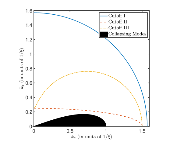
Figure 1: Cutoff I, is the cutoff used in this paper which has an isotropic from of $k_{c}=\pi/2\xi$. Cutoff II is the cutoff used in Bisset et al. (2016) which is given by $k_{c}(\vartheta)=1/\sqrt{\sin^{2}\vartheta/k_{c,\rho}^{2}+\cos^{2}\vartheta/k_{c,z}^{2}}$. Cutoff III is the cutoff used in Wächtler and Santos (2016) which is given by $k_{c}(\vartheta)=\sqrt{k_{c,\rho}^{2}\sin^{2}\vartheta+k_{c,z}^{2}\cos^{2}\vartheta}$, $\{k_{c,\rho},k_{c,z}\}=\{1.5,0.25\}\xi^{-1}$ for both options. Blackened region is the modes with imaginary energies when $\epsilon_{dd}=1.5$.

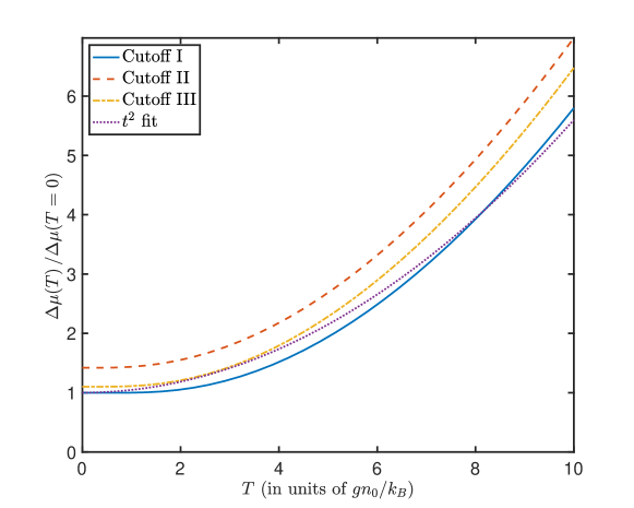
Figure 2: Temperature dependence of local LHY correction on the unitless temperature, $t=k_{B}T/gn_{0}$, calculated with different cutoff options for $\epsilon_{dd}=1.5$. Cutoff I is the spherical cutoff employed in this paper $\left(k_{c}^{\text{(I)}}=\pi/2\xi\right)$ (blue dotted line), Cutoff II, $k_{c}(\vartheta)^{\text{(II)}}=1/\sqrt{\sin^{2}\vartheta/k_{c,\rho}^{2}+\cos^{2}\vartheta/k_{c,z}^{2}}$ (orange dashed line), and Cutoff III, $k_{c}(\vartheta)^{\text{(III)}}=\sqrt{k_{c,\rho}^{2}\sin^{2}\vartheta+k_{c,z}^{2}\cos^{2}\vartheta}$ (yellow dash-dotted line), where $\{k_{c,\rho},k_{c,z}\}=\{1.5,0.25\}\xi^{-1}$are the anisotropic cutoffs used in Bisset et al. (2016) and Wächtler and Santos (2016) respectively. The $t^{2}$ fit used in the energy functional (Eq. 44) for the Cutoff I is also plotted (purple solid line).

Hence, at finite temperature the Bogoliubov amplitudes:

$$|v(\mathbf{x},\mathbf{k})|^{2} = \frac{\varepsilon_{\textbf{k}}+n_{0}(\mathbf{x})\tilde{V}_{\text{int}}(\mathbf{k})}{2E(\mathbf{x},\mathbf{k})}-\frac{1}{2}$$

$$u(\mathbf{x},\mathbf{k})v^{*}(\mathbf{x},\mathbf{k}) = \frac{n_{0}(\mathbf{x})\tilde{V}_{\text{int}}(\mathbf{k})}{2E(\mathbf{x},\mathbf{k})}$$ (26)

give the correction terms:

$$\Omega_{n}(\textbf{x})=\int\frac{d^{3}\textbf{k}}{(2\pi)^{3}}\tilde{V}_{\text{int}}(\textbf{k})\Big{\{}\frac{\varepsilon_{\mathbf{k}}+n_{0}(\mathbf{x})\tilde{V}_{\text{int}}(\mathbf{k})-E(\mathbf{x},\mathbf{k})}{2E(\mathbf{x},\mathbf{k})}+N(E(\textbf{x},\textbf{k}))\frac{\varepsilon_{\mathbf{k}}+n_{0}(\mathbf{x})\tilde{V}_{\text{int}}(\mathbf{k})}{E(\mathbf{x},\mathbf{k})}\Big{\}}$$ (27)

$$\Omega_{m}(\textbf{x})=\int\frac{d^{3}\textbf{k}}{(2\pi)^{3}}\tilde{V}_{\text{int}}(\textbf{k})\Big{\{}-\frac{n_{0}(\mathbf{x})\tilde{V}_{\text{int}}(\mathbf{k})}{2E(\mathbf{x},\mathbf{k})}+\frac{n_{0}(\mathbf{x})\tilde{V}_{\text{int}}(\mathbf{k})}{2\varepsilon_{\mathbf{k}}}-N(E(\textbf{x},\textbf{k}))\frac{n_{0}(\mathbf{x})\tilde{V}_{\text{int}}(\mathbf{k})}{E(\mathbf{x},\mathbf{k})}\Big{\}},$$ (28)

where the second term is properly renormalized. The local LHY correction becomes

$$\Delta\mu(\textbf{x})=\int\frac{d^{3}\textbf{k}}{(2\pi)^{3}}\tilde{V}_{\text{int}}(\textbf{k})\left\{\frac{\varepsilon_{\mathbf{k}}}{2E(\mathbf{x},\mathbf{k})}+\frac{n_{0}(\mathbf{x})\tilde{V}_{\text{int}}(\mathbf{k})}{2\varepsilon_{\mathbf{k}}}-\frac{1}{2}+\frac{1}{\exp\left[E(\mathbf{x},\mathbf{k})/k_{B}T\right]-1}\frac{\varepsilon_{\mathbf{k}}}{E(\mathbf{x},\mathbf{k})}\right\}.$$ (29)

Using

$$\xi(\textbf{x})=\sqrt{\frac{\hbar^{2}}{2Mgn_{0}(\textbf{x})}},$$ (30)

$k=q/\xi$, $\cos\vartheta=u$, $f(u)=1+\epsilon_{dd}\left(3u^{2}-1\right)$, and $t(\textbf{x})=\frac{k_{B}T}{gn_{0}(\textbf{x})}$, one can write

$$\Delta\mu(\textbf{x})=\frac{g}{4\pi^{2}\xi^{3}(\textbf{x})}\int_{-1}^{1}du\int_{q_{c}}^{\infty}q^{2}dqf(u)\Big{\{} \frac{q^{2}}{2\sqrt{q^{2}\left(q^{2}+2f(u)\right)}}+\frac{f(u)}{2q^{2}}-\frac{1}{2}$$ (31)

$$+\frac{1}{\exp\left[\sqrt{q^{2}\left(q^{2}+2f(u)\right)}/t(\textbf{x})\right]-1}\frac{q^{2}}{\sqrt{q^{2}\left(q^{2}+2f(u)\right)}}\Big{\}}.$$

Since $\xi\propto\Psi^{-1}$, the local change in the chemical potential is

$$\Delta\mu(\mathbf{x})=\frac{32}{3}g\sqrt{\frac{a_{s}^{3}}{\pi}}\left(\mathcal{Q}_{5}(\epsilon_{dd})+\mathcal{R}(\epsilon_{dd},t(\mathbf{x}))\right)|\Psi(\textbf{x})|^{3}.$$ (32)

Unitless functions $\mathcal{Q}_{5}$ and $\mathcal{R}$ are given by

$$\mathcal{Q}_{5}(\epsilon_{dd};q_{c})=\frac{1}{4\sqrt{2}}\int_{0}^{1}duf(u)\left[\left(4f(u)-q_{c}^{2}\right)\sqrt{2f(u)+q_{c}^{2}}-3f(u)q_{c}+q_{c}^{3}\right]$$ (33)

$$\mathcal{R}(\epsilon_{dd},t;q_{c})=\frac{3}{4\sqrt{2}}\int_{0}^{1}du\int_{q_{c}^{2}}^{\infty}dQ\frac{Qf(u)}{\sqrt{Q+2f(u)}}\frac{1}{\exp[\sqrt{Q\left(Q+2f(u)\right)}/t]-1}.$$ (34)

Within the same LDA, the depleted density is given by

$$\tilde{n}(\textbf{x})=\int\frac{d^{3}\textbf{k}}{(2\pi)^{3}}\left(|v(\textbf{x},\textbf{k})|^{2}+N_{B}(E(\textbf{x},\textbf{k}))\left[|u(\textbf{x},\textbf{k})|^{2}+|v(\textbf{x},\textbf{k})|^{2}\right]\right).$$ (35)

Using the Bogoliubov amplitudes given in Eq. III, one finds

$$\tilde{n}(\mathbf{x})=\frac{8}{3}g\sqrt{\frac{a_{s}^{3}}{\pi}}\left(\mathcal{Q}_{3}(\epsilon_{dd})+\mathcal{P}(\epsilon_{dd},t(\mathbf{x}))\right)|\Psi(\textbf{x})|^{3},$$ (36)

where

$$\mathcal{Q}_{3}(\epsilon_{dd};q_{c})=\frac{1}{\sqrt{2}}\int_{0}^{1}duf(u)\left[\left(f(u)-q_{c}^{2}\right)\sqrt{2f(u)+q_{c}^{2}}+q_{c}^{3}\right]$$ (37)

$$\mathcal{P}(\epsilon_{dd},t;q_{c})=\frac{3}{\sqrt{2}}\int_{0}^{1}du\int_{q_{c}^{2}}^{\infty}dQ\frac{Q+f(u)}{\sqrt{Q+2f(u)}}\frac{1}{\exp[\sqrt{Q\left(Q+2f(u)\right)}/t]-1}.$$ (38)

The non-condensate density increases with increasing temperature due to thermal depletion. In Fig. 3, temperature dependence of the non-condensate density is plotted. It is important to note that, near the edge of the condensate the unitless temperature increases as the condensate density decreases. Although the fraction of the non-condensate to the condensate density increases near the edge, total number of depleted atoms can remain small.

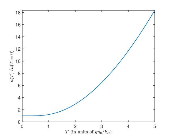
Figure 3: Non-condensate density $\tilde{n}(\mathbf{x})$ as a function of unitless temperature, $t=k_{B}T/gn_{0}$.

In the regime where the non-condensate density is negligible compared to condensate density, the generalized GP becomes:

$$\Big{[}h_{0}+\int d^{3}\mathbf{x}^{\prime}V_{\text{int}}(\mathbf{x}-\mathbf{x}^{\prime})|\Psi(\mathbf{x}^{\prime})|^{2}+\Delta\mu(\mathbf{x})\Big{]}\Psi(\mathbf{x})=0,$$ (39)

where $\Delta\mu(\mathbf{x})$ encompasses both quantum and thermal fluctuations:

$$\Delta\mu(\mathbf{x})=\frac{32}{3}g\sqrt{\frac{a_{s}^{3}}{\pi}}\left(\mathcal{Q}_{5}(\epsilon_{dd})+\mathcal{R}(\epsilon_{dd},t)\right)|\Psi(\mathbf{x})|^{3}.$$ (40)

Temperature fluctuation term $\mathcal{R}$ depends on the unitless temperature $t=k_{B}T/gn_{0}$. In Fig. 2, we display the temperature dependence of LHY correction for our cutoff choice. We check that other cutoff choices yield similar temperature dependencies.

In the next section we concentrate on the solution of this modified GP equation, particularly highlighting the effect of dramatic consequences of small but non-zero temperatures.

IV Variational Calculation of Temperature Dependent Density Profiles

As a first step to estimate the effects of temperature dependent LHY correction, we employ a Gaussian variational ansatz. Energy functional corresponding to the generalized GP equation (Eq. 13) is similar to what is used in Ref. Bisset et al. (2016). However, the thermal fluctuation term, $\mathcal{R}$, depends on condensate density through the unitless temperature. To get an analytical form for energy functional in $\Psi$, we used a power low fit for the $\mathcal{R}$ function. A $t^{n}$ curve for $n>2.5$ results in a divergence near the condensate edge where the condensate density is low and the unitless temperature is high. This divergence, however, is a byproduct of the Gaussian variational method, where the condensate extends to infinity. We find that a $t^{2}$ fit describes numerically obtained values within $0<t<10$ and results in a finite correction even when integrated over all space. In Fig. 2, we plot this fit with the function $\mathcal{R}$. The fit parameter in $\mathcal{R}(\epsilon_{dd},t)=S(\epsilon_{dd})t^{2}$ is found to be $\mathcal{S}(\epsilon_{dd})=-0.01029\epsilon_{dd}^{4}+0.02963\epsilon_{dd}^{3}-0.05422\epsilon_{dd}^{2}+0.009302\epsilon_{dd}+0.1698$ for $0<\epsilon_{dd}<2$.

Therefore, in the region where the depleted density is negligible compared to the condensate density, the generalized GP equation reads:

$$\left[-\frac{\hbar^{2}}{2M}\nabla^{2}+U_{\text{tr}}(\mathbf{x})+\int d^{3}\mathbf{x}^{\prime}V_{\text{int}}(\mathbf{x}-\mathbf{x}^{\prime})|\Psi(\mathbf{x}^{\prime})|^{2}+\gamma|\Psi(\mathbf{x})|^{3}+\theta T^{2}\frac{1}{|\Psi(\mathbf{x})|}\right]\Psi(\mathbf{x})=\mu\Psi(\mathbf{x}),$$ (41)

where $\gamma=\frac{32}{3}g\sqrt{\frac{a_{s}^{3}}{\pi}}\mathcal{Q}_{5}(\epsilon_{dd})$, and $\theta=\frac{32}{3}g\sqrt{\frac{a_{s}^{3}}{\pi}}\frac{k_{B}^{2}}{g^{2}}\mathcal{S}(\epsilon_{dd})$, and $\mathcal{S}$ is the found from the $t^{2}$ fit.

The energy functional corresponding to the generalized GP equation above is:

$$E[\Psi]= \int d^{3}\mathbf{x}\Psi^{*}(\mathbf{x})\left[-\frac{\hbar^{2}}{2M}\nabla^{2}+U_{\text{tr}}(\mathbf{x})\right]\Psi(\mathbf{x})$$

$$+\frac{1}{2}\int d^{3}\mathbf{x}\int d^{3}\mathbf{x^{\prime}}|\Psi(\mathbf{x})|^{2}V_{\text{int}}(\mathbf{x}-\mathbf{x}^{\prime})|\Psi(\mathbf{x}^{\prime})|^{2}$$

$$+\frac{2}{5}\int d^{3}\mathbf{x}\gamma|\Psi(\mathbf{x})|^{5}$$

$$+2\int d^{3}\mathbf{x}\theta T^{2}|\Psi(\mathbf{x})|.$$ (42)

To estimate the temperature effects on the condensate density profile, we used the Gaussian ansatz

$$\Psi(\mathbf{x})=\sqrt{\frac{8N}{\pi^{3/2}\sigma_{\rho}^{2}\sigma_{z}}}\exp\left[-2\left(\frac{\rho^{2}}{\sigma_{\rho}^{2}}+\frac{z^{2}}{\sigma_{z}^{2}}\right)\right].$$ (43)

For the trap potential $U_{\text{tr}}(\mathbf{x})=\frac{1}{2}M\left(\omega_{\rho}^{2}x^{2}+\omega_{\rho}^{2}y^{2}+\omega_{z}^{2}z^{2}\right)$, energy per particle for the above functional gives

$$\frac{E[\sigma_{\rho},\sigma_{z}]}{N} = \frac{\hbar^{2}}{M}\left(\frac{2}{\sigma_{\rho}^{2}}+\frac{1}{\sigma_{z}^{2}}\right)+M\left(\frac{\omega_{\rho}^{2}\sigma_{\rho}^{2}}{8}+\frac{\omega_{z}^{2}\sigma_{z}^{2}}{16}\right)$$ (44)

$$+ \frac{\sqrt{2}}{\pi^{3/2}}g\frac{N}{\sigma_{\rho}^{2}\sigma_{z}}\left[1-\epsilon_{dd}\mathcal{F}(\sigma_{\rho}/\sigma_{z})\right]$$

$$+ \frac{2^{12}}{75\sqrt{5}\pi^{11/4}}g\sqrt{a_{s}^{3}}\left(\frac{N}{\sigma_{\rho}^{2}\sigma_{z}}\right)^{3/2}\mathcal{Q}_{5}$$

$$+ \frac{64\pi^{1/4}}{3}\frac{k_{B}^{2}T^{2}}{g}\sqrt{a_{s}^{3}}\sqrt{\frac{\sigma_{\rho}^{2}\sigma_{z}}{N}}\mathcal{S},$$

where

$$\mathcal{F}(x)=\frac{1+2x^{2}}{1-x^{2}}-\frac{3x^{2}\tanh^{-1}\sqrt{1-x^{2}}}{\left(1-x^{2}\right)^{3/2}}.$$ (45)

We numerically find $\{\sigma_{\rho},\sigma_{z}\}$ which minimize this energy functional. Just as the zero temperature case Wächtler and Santos (2016); Bisset et al. (2016) two different kinds of minima can be observed corresponding to the trapped (low density) and the droplet (high density) phases. Increasing temperature may cause the system to shift from trapped phase to the droplet phase. In Fig. 4, we plot the radii of the condensate as a function of temperature, for a typical droplet reported in Kadau et al. (2016). It is important to note that the transition between the two phases happens close to $100$nK, and the total depletion at the center remains less than $8\%$ throughout.

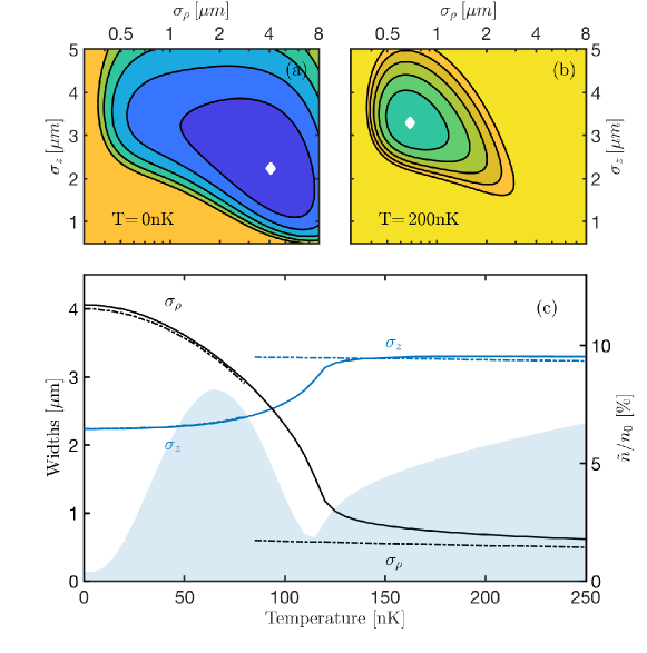
Figure 4: (a, b) Contour plots of total energy calculated with the energy functional Eq. 44 for $2000~{}^{164}$Dy atoms with $a_{dd}=132a_{0}$ and $a_{s}=93a_{0}$, where $a_{0}$ is the Bohr radius, at temperatures $T=0$ nK and $T=200$ nK, respectively. White diamonds show the energy minimum for the Gaussian ansatz. Results are for atoms in a harmonic trap with $\{\omega_{\rho},\omega_{z}\}=2\pi\times\{45,133\}s^{-1}$. (c) Variational radii of the stable condensate solutions for $a_{s}=88a_{0}$ (dash-dotted lines) and $a_{s}=93a_{0}$ (solid lines) at different temperatures for the same parameters as in (a,b). Shaded area corresponds to the depletion fraction at the center of the condensate calculated for the $a_{s}=93a_{0}$ case.

Stability of self bound droplets Schmitt et al. (2016) without a trapping potential is solely due to fluctuations. Hence, thermal fluctuations as well as quantum fluctuations determine their structure. Temperature dependence of their stability can be investigated with the same Gaussian ansatz. To estimate the central density, one writes the chemical potential at the condensate center

$$\left.\mu\right|_{\mathbf{r}=0}=gn_{0}\left(1-\epsilon_{dd}\mathcal{F}(\sigma_{\rho}/\sigma_{z})\right)+\gamma n_{0}^{3/2}+\theta T^{2}n_{0}^{-1/2}$$

as in Ref. Ferrier-Barbut et al. (2016). Therefore,

$$\left.\frac{\partial\mu}{\partial n_{0}}\right|_{\mathbf{r}=0}=g\left(1-\epsilon_{dd}\mathcal{F}(\sigma_{\rho}/\sigma_{z})\right)+\frac{3}{2}\gamma n_{0}^{1/2}-\frac{1}{2}\theta T^{2}n_{0}^{-3/2}.$$

The stability condition, $\partial\mu/\partial n_{0}\geq 0$, yields the equation for the minimum central density

$$0=\alpha+\frac{3}{2}\gamma n_{0}^{1/2}-\frac{1}{2}\theta T^{2}n_{0}^{-3/2},$$

where $\alpha=g\left(1-\epsilon_{dd}\mathcal{F}(\sigma_{\rho}/\sigma_{z})\right)$. At low temperatures, treating the temperature term as a perturbation, one gets

$$\sqrt{n_{0}}=-\frac{2\alpha}{3\gamma}-\frac{9\theta\gamma^{2}}{8\alpha^{3}}T^{2},$$ (46)

which, then, takes the form

$$n_{0}(T)=n_{0}(T=0)+\frac{2\mathcal{S}}{3\mathcal{Q}_{5}}\frac{k_{B}^{2}T^{2}}{g^{2}n_{0}(T=0)},$$ (47)

where $n_{0}(T=0)=\frac{\pi}{a_{s}^{3}}\left(\frac{\epsilon_{dd}\mathcal{F}(\sigma_{\rho}/\sigma_{z})-1}{16\mathcal{Q}_{5}}\right)^{2}$.

In Fig. 5, we plot the stable region in particle number and dipolar strength for self bound droplets at different temperatures. The minimum number of particles required to form a stable droplet increases with increasing temperature.

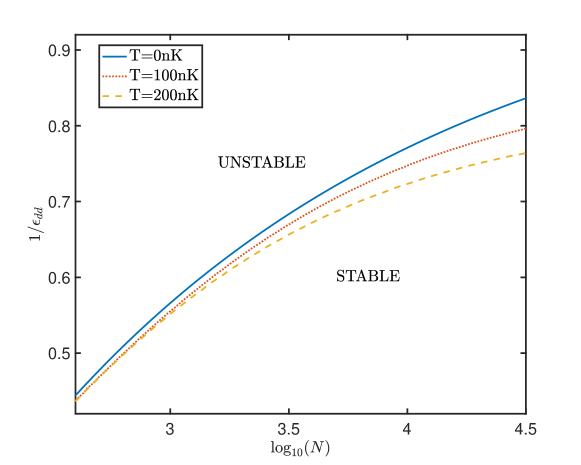
Figure 5: Phase diagram for self-bound droplets as a function of $1/\epsilon_{dd}$ and $N$ at $T=0$ nK (blue solid line), $T=100$ nK (orange dotted line) and $T=200$ nK (yellow dashed line).

V Conclusion

Let us summarize the main points of the calculation presented in the previous sections and their consequences. First, we derived the modified GP equation used in the literature to describe the dipolar droplets using HFBT and LDA applied to fluctuations. This derivation clarifies the assumptions inherent in the modified GP equation, and presents opportunities for systematic improvement. A consequence of this approach is that it constrains successful theoretical descriptions of systems where fluctuations are needed for equilibrium, in particular:

• Mean field description, as long as it takes the feedback of fluctuations back on the condensate as in HFBT, can be used to describe such fluctuation stabilized equilibria.

• HFBT equations, solved self consistently for the condensate and fluctuations can describe a stable droplet, without the introduction of ad-hoc terms to the local chemical potential.

• Popov approximation, which neglects anomalous non-condensed density is commonly used for trapped gases at finite temperature. However the terms neglected in this approximation provide a significant portion of the feedback on the condensate. Thus quantitatively accurate description of dipolar droplets are not possible within the Popov approximation.

• As the dipolar interaction is not short ranged, the correlations in the non-condensed density $\tilde{n}(\mathbf{x}^{\prime},\mathbf{x})$ are important. Setting $\tilde{n}(\mathbf{x}^{\prime},\mathbf{x})$ to a delta function before the local density approximation, as is commonly done for finite temperature numerical calculations, is bound to yield quantitatively incorrect results.

As a second point, using HFBT equations at finite temperature we generalized the description of dipolar droplets to finite temperatures. Our approach is limited to low enough temperatures so that the number of non-condensed particles are much smaller than the number of particles in the condensate, still our calculations indicate that:

• As the novel property of dipolar droplets is their stabilization by fluctuations, they become susceptible to temperature fluctuations even at low temperatures. The temperature scale at which the condensate sufficiently differs from zero temperature is set by comparing the thermally excited particle density with virtually excited particle density, not the condensed density.

• Temperature as low as to give a few percent of thermally excited density can drive the transition between trapped and dipolar phases in the current Dy experiments.

• Temperature does not have a straightforward effect on the droplet. While higher temperatures favor increasing density, such as the droplet phase over the low density phase in a trapö the minimum number of particles needed to stabilize a droplet also increases with increasing temperature.

Finally, we should outline the limitations of the theory given in this paper and how they can be overcome in future studies. First, the use of a variational wavefunction gives a rough measure of stability, but is not expected to be quantitatively correct, particularly in the droplet phase where the density may deviate significantly from a Gaussian. Instead of a variational wavefunction, direct numerical solution of the modified GP equation, including temperature corrections would be more accurate. We will report the results of such simulations in a follow upene . A second limitation of our calculation is that we neglected the interaction among the non-condensate particles. These interactions can be taken into account by self-consistent numerical solution of BdG equations, still within the LDA. Finally, our use of LDA forces a momentum space cutoff to exclude the unstable solutions. Any approach which takes the discrete nature of BdG modes at low energies into account would remove the need for such an arbitrary cutoff parameter. With such a precise characterization of temperature dependence, the density profile of dipolar droplets can be used to probe temperature in the nano-Kelvin regime.

This project is supported by Türkiye Bilimsel ve Teknolojik Araştırma Kurumu (TÜBİTAK) Grant No. 116F215.

References

Griesmaier et al. (2005)Axel Griesmaier, Jörg Werner, Sven Hensler,
Jürgen Stuhler, and Tilman Pfau, “Bose-Einstein Condensation of
Chromium,” Phys. Rev. Lett. 94, 160401 (2005).
Lu et al. (2011)Mingwu Lu, Nathaniel Q. Burdick, Seo Ho Youn,
and Benjamin L. Lev, “Strongly Dipolar
Bose-Einstein Condensate of Dysprosium,” Phys. Rev. Lett. 107, 190401 (2011).
Aikawa et al. (2012)K. Aikawa, A. Frisch,
M. Mark, S. Baier, A. Rietzler, R. Grimm, and F. Ferlaino, “Bose-Einstein Condensation of Erbium,” Phys. Rev. Lett. 108, 210401 (2012).
Kadau et al. (2016)Holger Kadau, Matthias Schmitt, Matthias Wenzel, Clarissa Wink,
Thomas Maier, Igor Ferrier-Barbut, and Tilman Pfau, “Observing the Rosensweig instability
of a quantum ferrofluid,” Nature 530, 194–197 (2016).
Chomaz et al. (2016)L. Chomaz, S. Baier,
D. Petter, M. J. Mark, F. Wächtler, L. Santos, and F. Ferlaino, “Quantum-Fluctuation-Driven Crossover from a Dilute
Bose-Einstein Condensate to a Macrodroplet in a Dipolar Quantum
Fluid,” Phys. Rev. X 6, 041039 (2016).
Ferrier-Barbut et al. (2016)Igor Ferrier-Barbut, Holger Kadau, Matthias Schmitt, Matthias Wenzel, and Tilman Pfau, “Observation of
Quantum Droplets in a Strongly Dipolar Bose Gas,” Phys. Rev. Lett. 116, 215301 (2016).
Schmitt et al. (2016)Matthias Schmitt, Matthias Wenzel, Fabian Böttcher, Igor Ferrier-Barbut, and Tilman Pfau, “Self-bound droplets of a dilute magnetic quantum liquid,” Nature 539, 259–262
(2016).
O’Dell et al. (2004)Duncan H. J. O’Dell, Stefano Giovanazzi, and Claudia Eberlein, “Exact Hydrodynamics of a Trapped Dipolar Bose-Einstein
Condensate,” Phys. Rev. Lett. 92, 250401 (2004).
Santos et al. (2003)L. Santos, G. V. Shlyapnikov, and M. Lewenstein, “Roton-Maxon Spectrum and Stability of Trapped Dipolar
Bose-Einstein Condensates,” Phys. Rev. Lett. 90, 250403 (2003).
Bisset and Blakie (2015)R. N. Bisset and P. B. Blakie, “Crystallization
of a dilute atomic dipolar condensate,” Phys.
Rev. A 92, 061603
(2015).
Xi and Saito (2016)Kui-Tian Xi and Hiroki Saito, “Droplet formation in a Bose-Einstein condensate with strong
dipole-dipole interaction,” Phys. Rev. A 93, 011604 (2016).
Wächtler and Santos (2016)F. Wächtler and L. Santos, “Quantum
filaments in dipolar Bose-Einstein condensates,” Phys.
Rev. A 93, 061603
(2016).
Lee et al. (1957)T. D. Lee, Kerson Huang, and C. N. Yang, “Eigenvalues and
Eigenfunctions of a Bose System of Hard Spheres and Its
Low-Temperature Properties,” Phys.
Rev. 106, 1135–1145
(1957).
Bisset et al. (2016)R. N. Bisset, R. M. Wilson,
D. Baillie, and P. B. Blakie, “Ground-state phase diagram of a dipolar
condensate with quantum fluctuations,” Phys.
Rev. A 94, 033619
(2016).
Griffin (1996)A. Griffin, “Conserving and
gapless approximations for an inhomogeneous Bose gas at finite
temperatures,” Phys. Rev. B 53, 9341–9347 (1996).
Giorgini et al. (1996)S. Giorgini, L. P. Pitaevskii, and S. Stringari, “Condensate
fraction and critical temperature of a trapped interacting Bose gas,” Phys. Rev. A 54, R4633–R4636 (1996).
Jin et al. (1997)D. S. Jin, M. R. Matthews,
J. R. Ensher, C. E. Wieman, and E. A. Cornell, “Temperature-Dependent Damping and
Frequency Shifts in Collective Excitations of a Dilute
Bose-Einstein Condensate,” Phys.
Rev. Lett. 78, 764–767
(1997).
Ronen and Bohn (2007)Shai Ronen and John L. Bohn, “Dipolar
Bose-Einstein condensates at finite temperature,” Phys.
Rev. A 76, 043607
(2007).
Lima and Pelster (2012)A. R. P. Lima and A. Pelster, “Beyond
mean-field low-lying excitations of dipolar Bose gases,” Phys.
Rev. A 86, 063609
(2012).
Wächtler and Santos (2016)F. Wächtler and L. Santos, “Ground-state
properties and elementary excitations of quantum droplets in dipolar
Bose-Einstein condensates,” Phys.
Rev. A 94, 043618
(2016).
(24)E. Aybar, Ş.F. Öztürk, and M.
Ö. Oktel, to be published.