GENERALIZED DARK MATTER MODEL WITH THE EUCLID SATELLITE

Abstract

The concordance model in cosmology, $\Lambda$CDM, is able to fit the main cosmological observations with a high level of accuracy. However, around 95% of the energy content of the Universe within this framework remains still unknown. In this work we focus on the dark matter component and we investigate the generalized dark matter (GDM) model, which allows for non-pressure-less dark matter and a non-vanishing sound speed and viscosity. We first focus on current observations, showing that GDM could alleviate the tension between cosmic microwave background and weak lensing observations. We then investigate the ability of the photometric Euclid survey (photometric galaxy clustering, weak lensing, and their cross-correlations) to constrain the nature of dark matter. We conclude that Euclid will provide us with very good constraints on GDM, enabling us to better understand the nature of this fluid, but a non-linear recipe adapted to GDM is clearly needed in order to correct for non-linearities and get reliable results down to small scales.

1 Introduction

$\Lambda$CDM has become the concordance model in cosmology thanks to its ability to fit the main cosmological observations [1]. It is mainly characterized by its dark sector, composed of pressure-less, non-interacting cold dark matter (CDM) and a cosmological constant $\Lambda$. However, their nature remain still unknown. In this work we focus only on the dark matter component of the Universe and we follow a phenomenological approach to go beyond the standard model. In particular, we use the generalized dark matter (GDM) model, first proposed by Hu [2], to constrain dark matter properties in the linear regime. We first present the theoretical framework of the GDM model in Sec. 2. We then show the constraints on this model using current observations in Sec. 3, and we finally show the expected precision of the photometric Euclid survey on the GDM model parameters in Sec. 4, before finishing with the conclusions in Sec. 5.

2 Theoretical framework

In this work we assume that dark matter is only coupled to the visible sector through gravitational interaction, so we assume that the dark matter energy-momentum tensor is conserved. This implies that all kind of dark matter components can be covered by the standard conservation equations for a general matter source [3]. The dark matter energy density $\rho$ evolves as $\dot{\rho}+3H(1+w)\rho=0$, where the over-dot stands for the derivative with respect to conformal time, and $H\equiv\dot{a}/a$ is the conformal Hubble parameter. In this work we focus on the scalar modes, neglecting vector and tensor perturbations. Therefore, a conserved energy-momentum tensor must satisfy [3] (at a linear level of perturbations and in the synchronous gauge)

$$\dot{\delta}+(1+w)\left(\theta+\frac{\dot{h}}{2}\right)+3H\left(\frac{\delta p}{\delta\rho}-w\right)=0\,\hskip 5.0pt{\rm and}\hskip 5.0pt\dot{\theta}+H(1-3w)\theta+\frac{\dot{w}}{1+w}\theta-\frac{\delta p/\delta\rho}{1+w}k^{2}\delta+k^{2}\sigma=0\,,$$ (1)

where $w$, $\delta$, and $\theta$ stand for the fluid equation of state parameter, its density fluctuation and the divergence of its velocity, respectively. $\delta p$ represents the pressure perturbation, and $\sigma$ corresponds to the anisotropic stress. Provided Eq. (1), the GDM model is specified by the dark matter equation of state parameter $w$, and relations between $\delta p$ and $\sigma$ to the dynamically evolving variables $\delta,\,\theta$. We consider non-relativistic dark matter (it can allow for the formation of galaxies) with the so-called $c_{\rm vis}$ parametrization [2], where $\delta p$ is related to $\delta$ and $\theta$ through the rest-frame sound speed $c_{s}$, and $\sigma$ evolves according to:

$$\delta p=c_{s}^{2}\delta\rho-\dot{\rho}(c_{s}^{2}-c_{a}^{2})\theta/k^{2}\,\hskip 5.0pt{\rm and}\hskip 5.0pt\dot{\sigma}+3H\frac{c_{a}^{2}}{w}\sigma=\frac{4}{3}\frac{c_{\rm vis}^{2}}{1+w}(2\theta+\dot{h}+6\dot{\eta})\,,$$ (2)

where the adiabatic sound speed is $c_{a}^{2}\equiv(w\rho)^{\dot{}}/\dot{\rho}$, $c_{\rm vis}^{2}$ is a new viscosity parameter, and $h$ and $\eta$ are the synchronous metric perturbations. We fix $c_{\rm vis}^{2}=0$, for simplicity, and we consider only the equation of state parameter $w$ and the sound velocity $c_{s}^{2}$ as constant parameters for the GDM model.

3 Current constraints

We first need a Boltzmann code to compute the power spectrum for the GDM model. In this work we use the CLASS code [4]. It already includes a parametrization for the dark energy fluid with a constant equation of state parameter and a constant sound velocity [5], so we use this parametrization as GDM, while we keep a cosmological constant for the dark energy contribution, and a negligible fraction of cold dark matter. Notice that the perturbations computed for this fluid must be added to the total matter perturbations, which is not the case in the default version of CLASS, since the fluid is supposed to behave as dark energy. We then investigate the constraints on the cosmological parameters using a Markov chain Monte Carlo approach, with the Metropolis-Hastings algorithm, implemented in the parameter inference Monte Python code [6]. We use the Gelman-Rubin test [7], requiring $1-R<0.015$ for all parameters, to consider that the chains have converged. We consider the 6 baseline parameters for $\Lambda$CDM that can be seen in Table 1, plus $w$ and $c_{s}^{2}$ for GDM. We further consider two massless neutrinos and a massive one with mass 0.06 eV, keeping the value of the effective number of neutrino-like relativistic degrees of freedom $N_{\rm eff}=3.046$. The constraints on the parameters are obtained using CMB data (the 2015 Planck CMB likelihoods [8, 9]), baryon acoustic oscillations (BAO) measurements from BOSS [10], 6dFGS [11], and SDSS [12], and type Ia supernovae (SNIa) data from the joint light-curve analysis (JLA) [13]. For some runs we include weak lensing (WL) data from the CFHTLenS survey [14] to check whether the tension between WL and CMB data is alleviated when considering GDM.

In Table 1 we present the constraints on the cosmological parameters when we fit both models, $\Lambda$CDM and $\Lambda$GDM, to SNIa, BAO, and CMB data. The constraints are weakened when we consider $\Lambda$GDM, due to the introduction of two extra degrees of freedom. Even if all the parameters are compatible within 1-$\sigma$ for both models, we can see that $\Lambda$GDM allows for a smaller value of $\Omega_{\rm b}$, $\Omega_{\rm dm}$ and $\sigma_{8}$, and a larger value of $h$ than $\Lambda$CDM. This points towards the fact that $\Lambda$GDM could alleviate the tension between $\Omega_{\rm m}$ and the rms matter density fluctuation $\sigma_{8}$ that appears when considering the $\Lambda$CDM model, as it can be seen in the left panel of Fig. 1. Allowing for a non-vanishing sound speed strongly suppresses the matter power spectrum at small scales, therefore, cosmological probes sensitive to small scales are extremely important to constrain the GDM parameters. In order to add WL data we need to take into account that we enter the non-linear regime and our predictions for GDM are no longer accurate. There is no non-linear recipe for GDM yet, so we use an ultra-conservative approach by keeping only the largest scales from CFHTLenS data, and we keep the standard halofit [15] non-linear correction. The constraints when WL data is added into the analysis are shown in Table 1. We can observe that the constraints on most of the parameters (for both models) are equivalent to the ones obtained without WL, since we are discarding most of the WL data. However, the constraint on $c_{s}^{2}$ improves by two orders of magnitude, due to the addition of information at mildly non-linear scales. We need to remind, though, that the halofit correction has been derived and tested only for standard cold dark matter, so the constraint on $c_{s}^{2}$ could be slightly too optimistic. We can also see this effect in the right panel of Fig. 1. The (probably) over-estimated spectrum at small scales for $\Lambda$GDM gives very good constraints on $\sigma_{8}$, questioning the ability of $\Lambda$GDM to completely remove the tension between WL and CMB measurements.

Table 1: Mean values with the 1-$\sigma$ constraints on the cosmological parameters for both $\Lambda$CDM and $\Lambda$GDM. Both the constraints from the fit to CMB, SNIa, and BAO data (with and without WL) and the forecasted constraints from the photometric Euclid survey are shown.

Model	Parameters	CMB+SNIa+BAO	CMB+SNIa+BAO+WL	Photometric Euclid
	$10^{2}\times\Omega_{\rm b}$	$4.834\pm 0.054$	$4.815\pm 0.053$	$(4.834)\pm 0.075$
	$\Omega_{\rm dm}$	$0.2562\pm 0.0060$	$0.2539\pm 0.0057$	$(0.2562)\pm 0.0074$
$\Lambda$CDM	$h$	$0.6797\pm 0.0049$	$0.6816\pm 0.0048$	$(0.6797)\pm 0.016$
	$\sigma_{8}$	$0.8187\pm 0.0089$	$0.8142\pm 0.0090$	$(0.8187)\pm 0.0088$
	$n_{s}$	$0.9674\pm 0.0043$	$0.9686\pm 0.0043$	$(0.9674)\pm 0.023$
	$10\times\tau$	$0.72\pm 0.13$	$0.68\pm 0.13$	$-$
	$10^{2}\times\Omega_{\rm b}$	$4.71\pm 0.12$	$4.69\pm 0.12$	$(4.834)\pm 0.11$
	$\Omega_{\rm dm}$	$0.2491\pm 0.0087$	$0.2458\pm 0.0088$	$(0.2562)\pm 0.014$
	$10^{2}\times w$	$0.066\pm 0.054$	$0.055\pm 0.053$	$(0.00)\pm 0.21$
$\Lambda$GDM	$10^{6}\times c_{s}^{2}$	$<0.78$	$<0.010$	$<0.0018$
	$h$	$0.6873\pm 0.0082$	$0.6898\pm 0.0082$	$(0.6797)\pm 0.020$
	$\sigma_{8}$	$0.7351_{-0.041}^{+0.094}$	$0.8174\pm 0.016$	$(0.8187)\pm 0.0096$
	$n_{s}$	$0.9656\pm 0.0044$	$0.9682\pm 0.0042$	$(0.9674)\pm 0.035$
	$10\times\tau$	$0.73\pm 0.15$	$0.58\pm 0.16$	$-$

4 Euclid forecast

In this section we focus our attention to study the $\Lambda$GDM model with the future Euclid satellite  using the specifications of the Euclid Red-book [16]. We use the CosmoSIS [17] code  to compute a Fisher matrix forecast for the photometric Euclid survey. In particular, for photometric galaxy clustering (GC), weak lensing (WL), and their cross-correlations (XC). More in detail, we replace (in the CosmoSIS pipeline) the standard Boltzmann code by our GDM modified version of CLASS used in the previous section. We follow the previous approach of using the halofit correction and keeping only the largest scales (up to $\ell_{\rm max}=750$). Concerning the fiducial cosmological model for the forecast, we use the values obtained from the fit of $\Lambda$CDM to the combination of CMB, SNIa, and BAO data from the previous section, including the treatment of massive neutrinos and the value of $\tau$, which are fixed in the forecast. For the parameters specific to GDM we consider the fiducial values $w=0$ and $c_{s}^{2}=10^{-9}$.

We can see in Table 1 that the photometric Euclid survey will provide very good constraints on all parameters for both models. For some parameters the forecasted constraints are worse than the current ones. but this can be justified by the fact that Euclid will only probe up to redshift $\sim 2.5$. Therefore, the lack of high-redshift information coming from the CMB makes it harder to constrain $w$ and break the degeneracies between the cosmological parameters. We can infer that the combination of the full (photometric and spectroscopic) Euclid data with the CMB will provide exquisite constraints on GDM. It is worth mentioning that current low-redshift probes (without the CMB) are only marginally able to constrain the GDM parameters [18]. It is also important to notice that the photometric Euclid survey alone will be able to constrain $c_{s}^{2}$ better than the combination of background and WL current data by nearly an order of magnitude. However, as it was the case in the previous section, we should treat these forecasted constraints (especially on $c_{s}^{2}$) with caution, since we know that the halofit correction is adapted to standard cold dark matter.

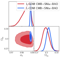
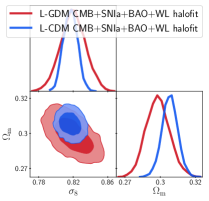
Figure 1: 1-$\sigma$ and 2-$\sigma$ contours for the $\Omega_{\rm m}$ and $\sigma_{8}$ cosmological parameters for both $\Lambda$CDM (blue) and $\Lambda$GDM (red). Left panel: Combination of CMB, SNIa, and BAO data. Right panel: WL data are added into the analysis.

5 Conclusions

In conclusion, we have seen that a more generalized treatment of dark matter could alleviate the tension between low-redshift and high-redshift data, thanks to a non-vanishing sound speed. Because of $c_{s}^{2}$, the main differences between GDM and the standard model appear at small scales. It is thus very important to add cosmological probes sensitive to small scales to constrain GDM. We have shown that adding WL data strongly improves the constraints on the GDM sound speed. We have then focused on the photometric Euclid survey, and we have shown that it will be able to put nice constraints on all parameters (a very strong constraint on $c_{s}^{2}$), and it will allow us to increase our knowledge on the nature of dark matter. However, it is necessary to have a non-linear recipe adapted to GDM to be able to explore the small scales that Euclid will probe, and extract the maximum of information of it.

References

References

- [1] Planck Collaboration, A&A 594, A13 (2016).
- [2] W. Hu, ApJ 506, 485 (1998).
- [3] C.-P. Ma & E. Bertschinger, ApJ 455, 7 (1995).
- [4] D. Blas, J. Lesgourgues, & T. Tram JCAP 07, 034 (2011).
- [5] J. Lesgourgues & T. Tram, JCAP 09, 032 (2011).
- [6] B. Audren et al., JCAP 02, 001 (2013).
- [7] A. Gelman & D. B. Rubin, Statist. Sci. 7, 457 (1992).
- [8] Planck Collaboration, A&A 594, A11 (2016).
- [9] Planck Collaboration, A&A 594, A15 (2016).
- [10] L. Anderson et al., MNRAS 441, 24 (2014).
- [11] F. Beutler et al., MNRAS 416, 3017 (2011).
- [12] A. J. Ross et al., MNRAS 449, 835 (2015).
- [13] M. Betoule et al., A&A 568, A22 (2014).
- [14] C. Heymans et al., MNRAS 432, 2433 (2013).
- [15] R. Takahashi et al., ApJ 761, 152 (2012).
- [16] R. Laureijs et al., ArXiv e-prints arXiv, 1110.3193 (2011).
- [17] J. Zuntz et al., A&C 12, 45 (2015).
- [18] I. Tutusaus et al., PRD 94, 123515 (2016).