Self-bound Bose mixtures

Abstract

Recent experiments confirmed that fluctuations beyond the mean-field approximation can lead to self-bound liquid droplets of ultra-dilute binary Bose mixtures. We proceed beyond the beyond-mean-field approximation, and study liquid Bose mixtures using the variational hypernetted-chain Euler Lagrange method, which accounts for correlations non-perturbatively. Focusing on the case of a mixture of uniform density, as realized inside large saturated droplets, we study the conditions for stability against evaporation of one of the components (both chemical potentials need to be negative) and against liquid-gas phase separation (spinodal instability), the latter being accompanied by a vanishing speed of sound. Dilute Bose mixtures are stable only in a narrow range near an optimal ratio $\rho_{1}/\rho_{2}$ and near the total energy minimum. Deviations from a universal dependence on the $s$-wave scattering lengths are significant despite the low density.

Ultracold quantum gases provide a rich toolbox to study correlations in quantum many-body systems Bloch et al. (2008) and model condensed matter physics such as magnetic systems Micheli et al. (2006), solid state systems Bloch (2005), or superfluidity Randeria et al. (2012). A recent example is the prediction Petrov (2015) and two independent observations Cabrera et al. (2018); Semeghini et al. (2017) of a self-bound liquid mixture of two ultra-dilute Bose gases (³⁹K atoms in two different hyperfine states). In this liquid state, when the attraction between different species overcomes the single-species average repulsion, the mean-field approach Dalfovo et al. (1999) would predict a collapse. In Ref. Petrov (2015), correlations were taken into account approximatively using the beyond-mean-field (BMF) approximation Larsen (1963). In a regime where the BMF corrections can stabilize the binary mixture by compensation of the mean-field attraction, self-bound droplets are formed which live long enough to perform measurements with the trapping potential switched off. Being self-bound and three-dimensional, they are different from bright solitons, which are essentially one-dimensional and have a limited number of particles Cheiney et al. (2018), while droplets can only be formed with a critical minimum number of atoms. On a similar footage, self-bound droplets in the region of mean-field collapse have also been found in dipolar trapped systems of ¹⁶⁴Dy Kadau et al. (2016a); Ferrier-Barbut et al. (2016a); Schmitt et al. (2016) and ¹⁶⁶Er Chomaz et al. (2016) atoms. In this case quantum fluctuations compensate the attractive components of the dipolar interactions, as confirmed by theory Wächtler and Santos (2016); Bombin et al. (2017). Bose mixtures and dipolar Bose gases share similarities (competition between repulsive and attractive interactions), although the latter case is complicated by the anisotropy of the dipolar interaction.

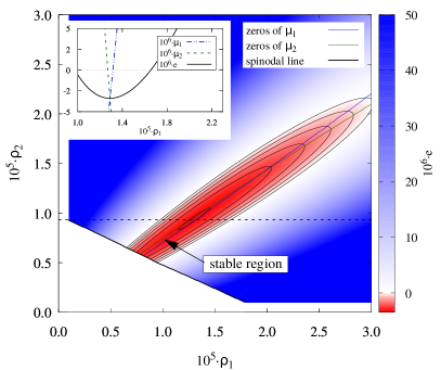
Figure 1: (Color online) Total energy per particle $e$ as function of $\rho_{1}$ and $\rho_{2}$, with contour lines for energies -3.35, -2.68, -2.01, -1.34, -0.67, and 0.0 Also shown are the spinodal instability (thick black line), and the zeroes of the chemical potentials $\mu_{1}$ (blue) and $\mu_{2}$ (green). Only in the narrow region pointed at by the arrow the mixture is stable against evaporation. The inset shows $e$ and the chemical potentials $\mu_{1}$ and $\mu_{2}$ along the dashed line intersecting the energy minimum.

A large enough, saturated droplet has a surface region, where the density drops to zero, and a uniform interior, with a density plateau at the equilibrium density $\rho_{\rm eq}$ resulting from the balance of attractive and repulsive interactions. In this work we focus on the effect of self-binding rather than on the droplet surface. Therefore we take the thermodynamic limit, $N\to\infty$ and $V\to\infty$, with $\rho=N/V$ fixed. We investigate the ground state of a three-dimensional uniform Bose mixture with partial densities $\rho_{1}$ and $\rho_{2}$ (hence a total density $\rho=\rho_{1}+\rho_{2}$), and equal atom masses $m$. We explore a wide range of $\rho_{1}$ and $\rho_{2}$ values, finding an optimal ratio $\rho_{1}/\rho_{2}$ and the equilibrium density $\rho_{\rm eq}$. We note, however, that in the presently published experiments Cabrera et al. (2018); Semeghini et al. (2017), the self-bound droplets are not saturated: they do not exhibit a central density plateau, but an approximately Gaussian density profile, and are so small that they are dominated by surface effects.

The Hamiltonian of a Bose mixture is given by

$$H=\sum_{i,\alpha}{\hbar^{2}\over 2m}\Delta_{i,\alpha}+{1\over 2}\sum_{\alpha,\beta}\sideset{}{{}^{\prime}}{\sum}_{i,j}v_{\alpha,\beta}(|{\bf r}_{i,\alpha}-{\bf r}_{j,\beta}|)$$ (1)

where a Greek index $\alpha$ labels the component, and a Latin index $i$ numbers the atoms of species $\alpha$. The prime indicates that we only sum over $i\neq j$ for $\alpha=\beta$. We use the Lennard-Jones-like interactions

$$v_{\alpha,\beta}(r)=s_{\alpha,\beta}\left[\Big{(}{\sigma_{\alpha,\beta}\over r}\Big{)}^{10}-\Big{(}{\sigma_{\alpha,\beta}\over r}\Big{)}^{6}\right]\ ,$$

with $v_{12}=v_{21}$. The parameters of $v_{\alpha,\beta}$ are adjusted to set the $s$-wave scattering length $a_{\alpha,\beta}$ to a desired value, which can be done analyticallyPade (2007). Since $v_{\alpha,\beta}$ has two parameters, we further characterize $v_{\alpha,\beta}(r)$ by the effective range $r_{\alpha,\beta}^{\rm eff}$, evaluated numerically Buendia et al. (1984). In all calculations, $s_{\alpha,\beta}$ and $\sigma_{\alpha,\beta}$ are chosen such that there are no two-body bound states.

Previously, Lee-Huang-Yang corrections to the mean-field approximation Petrov (2015) and quantum Monte Carlo (QMC) methods Petrov and Astrakharchik (2016); Cikojevic et al. (2018) have been employed. Here we use a different approach, the variational hypernetted-chain Euler Lagrange (HNC-EL) method. HNC-EL is computationally very economical like the BMF approximation, but has the advantage of including correlations in a non-perturbative manner. This leads to a strictly real ground state energy, in contrast to the BMF approximation where the energy of a uniform self-bound mixture has an unphysical small imaginary part. The two-component HNC-EL method has been described in Ref. Chakraborty (1982) and in a different formulation in Ref. Campbell (1972), and has been recently generalized to multi-component Bose mixtures Hebenstreit et al. (2016). The starting point is the variational Jastrow-Feenberg ansatz Feenberg (1969) for the ground state consisting of a product of pair correlation functions for a multi-component Bose system,

$$\Psi_{0}(\{{\bf r}_{i,\alpha}\})=\exp\Big{[}{1\over 4}\sum_{\alpha,\beta}\sideset{}{{}^{\prime}}{\sum}_{i,j}u_{\alpha,\beta}(|{\bf r}_{i,\alpha}-{\bf r}_{j,\beta}|)\Big{]}\ .$$ (2)

The many-body wave function $\Psi_{0}$ does not contain one-body functions $u_{\alpha}({\bf r}_{i,\alpha})$ because we consider a uniform system. Higher order correlations such as triplets $u_{\alpha,\beta,\gamma}({\bf r}_{i,\alpha},{\bf r}_{j,\beta},{\bf r}_{k,\gamma})$ have been incorporated approximately for helium Fabrocini and Polls (1984); Krotscheck (1986), but are neglected here because their contribution is very small at low density.

We solve the Euler-Lagrange equations $\delta e/\delta g_{\alpha,\beta}(r)=0$, where the energy per particle $e={1\over N}{\langle\Psi_{0}|H|\Psi_{0}\rangle\over\langle\Psi_{0}|\Psi_{0}\rangle}$ is

$$e=\sum_{\alpha,\beta}{\rho_{\alpha}\rho_{\beta}\over 2\rho}\int d^{3}r\,g_{\alpha,\beta}(r)\big{[}v_{\alpha,\beta}(r)-{\hbar^{2}\over 4m}\Delta u_{\alpha,\beta}(r)\big{]}$$ (3)

in terms of the pair distribution function

$$g_{\alpha,\beta}(r)={1+\delta_{\alpha\beta}\over\rho_{\alpha}\rho_{\beta}}{\delta\ln\langle\Psi_{0}|\Psi_{0}\rangle\over\delta u_{\alpha,\beta}}\ .$$

Partial summation of the Meyer cluster diagrams for $\ln\langle\Psi_{0}|\Psi_{0}\rangle$ in the HNC/0 approximation provides a relation between $g_{\alpha,\beta}$ and $u_{\alpha,\beta}$ Hansen and McDonald (1986); Hebenstreit (2013). A practical formulation of the resulting HNC-EL equations to be solved for $g_{\alpha,\beta}$ can be found in Ref. Hebenstreit et al. (2016). From $g_{\alpha,\beta}(r)$ we can calculate the static structure functions $S_{\alpha,\beta}(k)=\delta_{\alpha\beta}+\sqrt{\rho_{\alpha}\rho_{\beta}}\ {\rm FT}[g_{\alpha,\beta}-1]$ (FT denotes Fourier transformation), needed for the calculation of excitations.

At low densities, a uniform binary Bose mixture of two species of equal mass is characterized by the scattering lengths $a_{11}$, $a_{12}$, and $a_{22}$, and the partial densities $\rho_{1}$ and $\rho_{2}$. However, our results depend also on the next term in the expansion of the scattering phase shift, the effective range $r_{\alpha,\beta}^{\rm eff}$ Landau and Lifshitz (1958) leading to a total of 8 parameters $\{\rho_{\alpha},a_{\alpha,\beta},r_{\alpha,\beta}^{\rm eff}\}$ to characterize our uniform binary Bose mixtures. We use $a_{11}$ as length unit and $E_{0}\equiv\hbar^{2}/ma_{11}^{2}$ as energy unit. For ${}^{39}K$ used in experiments Cabrera et al. (2018); Semeghini et al. (2017), we have $a_{11}=35.2a_{B}$ and $E_{0}=3.55$mK.

We use the combinations of scattering lengths $a_{\alpha\beta}$ from the experiments reported in Ref. Cabrera et al. (2018), which are very similar to those in Ref. Semeghini et al. (2017). A negative value of $\delta a=a_{12}+\sqrt{a_{11}a_{22}}$ is necessary for a self-bound mixture. Before investigating the dependence on $\delta a$, we study the dependence on the partial densities $\rho_{1}$ and $\rho_{2}$. Fig. 1 shows a map of the energy per particle $e$ as function of $\rho_{1}$ and $\rho_{2}$ for the experimental scattering length values corresponding to $\delta a=-5.5a_{B}$, which is $\delta a=-0.156$ in our length unit $a_{11}$ and the most negative value in Ref. Cabrera et al. (2018). The other scattering lengths are $a_{22}=1.86$ and $a_{12}=-1.52$. The effective ranges are $r_{11}^{\rm eff}=5.2$, $r_{12}^{\rm eff}=33.0$, and $r_{22}^{\rm eff}=43.2$. Negative energies, where the mixture is a self-bound liquid, are shown by a red color range, together with contour lines, positive energies by a blue color range. Thus, as predicted by BMF calculations Petrov (2015) and confirmed by experiments Cabrera et al. (2018); Semeghini et al. (2017), we find a liquid state for $\delta a<0$. In the phase space $(\rho_{1},\rho_{2})$ the self-bound states form a narrow valley following a typical optimal ratio $\rho_{1}/\rho_{2}$. The phase space of meaningful combinations $(\rho_{1},\rho_{2})$ ends at the spinodal line (thick black line in Fig.1). Approaching this line, the uniform mixture becomes sensitive to long-wavelength density oscillations (see below). At the spinodal line infinitesimal density fluctuations trigger a liquid-gas phase separation.

While in a uniform mixture we can choose any $\rho_{1}$ and $\rho_{1}$, a finite droplet adjusts its radius to minimize the energy, attaining the equilibrium (zero pressure) density inside the droplet. The situation is more complicated for a mixture because the droplet radius affects only the total density, but not necessarily the ratio $\rho_{1}/\rho_{2}$. The latter can be adjusted by evaporating one component or by phase separation. Therefore we calculate the chemical potential of component $\alpha$, $\mu_{\alpha}(\rho_{1},\rho_{2})=e(\rho_{1},\rho_{2})+\rho{\partial e(\rho_{1},\rho_{2})\over\partial\rho_{\alpha}}$. If $\mu_{\alpha}>0$ a particle of species $\alpha$ is not bound to the mixture – the energy is lowered by removing it. A stable droplet requires both $e<0$ (red valley in Fig.1) and $\mu_{\alpha}<0$. The blue line in Fig.1 are the zeroes of $\mu_{1}$, with $\mu_{1}<0$ above this line. Similarly the green line are the zeroes of $\mu_{2}$, with $\mu_{2}<0$ below this line. Hence only the narrow region pointed at by the arrow is stable against evaporation; this region includes of course the equilibrium energy $e_{\rm eq}=\min[e]$. The inset of Fig.1 shows $e$, $\mu_{1}$ and $\mu_{2}$ along the dashed line as function of $\rho_{1}$ for a fixed value $\rho_{2}a_{11}^{3}=0.934$, such that we intersect the equilibrium energy. $\mu_{\alpha}$ is very sensitive to the partial density, which explains why the region where both $\mu_{\alpha}<0$ is so narrow. If a droplet is prepared outside the stable region, particles evaporate and the system moves on the energy surface until it is stable.

Our results for $e$ and $\mu_{\alpha}$ mean that large droplets will reach the equilibrium energy $e_{\rm eq}$ by a combination of evaporating superfluous particles and adjusting the droplet radius. In the case discussed so far, $\delta a=-0.156$, the density ratio at the equilibrium energy predicted from our HNC-EL results in Fig.1) is $\rho_{1}/\rho_{2}=1.380$, which is to be compared with the optimal mean-field ratio Pethick and Smith (2008) $\rho_{1}/\rho_{2}=\sqrt{a_{22}/a_{11}}=1.363$. The latter is a very good approximation even though the mean-field approximation does not even predict a liquid state. As seen in the inset of Fig.1, $e$ changes very little if the density ratio is slightly changed; therefore for further calculations of $e$ we use the mean-field ratio.

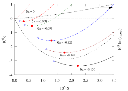
Figure 2: (Color online) Energy per particle $e$ as function of the total density $\rho$ for several values $\delta a$. Closed circles denote the equilibrium density $\rho_{\rm eq}$ and energy $e_{\rm eq}$; open circles denote spinodal points. The black dashed and dash-dotted lines are the real and imaginary parts, the latter using a different scale, of the BMF energy for $\delta a=-0.156$.

$\delta a[a_{B}]$	$\delta a$	$a_{22}$	$r_{22}^{\rm eff}$	$\rho_{1}/\rho_{2}$	$10^{6}e_{\rm eq}$	$10^{5}\rho_{\rm eq}$
$-5.5$	$-0.156$	$1.86$	$43.2$	$1.363$	$-3.364$	$2.221$
$-5.0$	$-0.142$	$1.90$	$40.3$	$1.377$	$-2.426$	$1.756$
$-4.4$	$-0.125$	$1.94$	$37.0$	$1.394$	$-1.571$	$1.294$
$-3.2$	$-0.091$	$2.04$	$31.2$	$1.428$	$-0.544$	$0.609$
$-2.4$	$-0.068$	$2.10$	$27.7$	$1.450$	$-0.214$	$0.319$
$0.0$	$0.0$	$2.31$	$19.1$	$1.519$	–	–

Table 1: Values for $\delta a$, $a_{22}$, $r_{22}^{\rm eff}$, and $\rho_{1}/\rho_{2}$ used to obtain the results shown in Fig. 2, as well as the equilibrium energy and density obtained from these results. Lengths and energies are in units of $a_{11}$ and $E_{0}$ (see text) if not otherwise stated.

When $\delta a$ increases towards zero, the liquid becomes less bound, until it is no longer self-bound at $\delta a=0$. In Fig. 2 the energy per particle $e$ as function of total density $\rho$ is shown for several values of $\delta a$ in the range $[-0.156,0]$, corresponding to the range of values in experiments Cabrera et al. (2018); Semeghini et al. (2017) where $\delta a$ is adjusted by changing the $s$-wave scattering length $a_{22}$ via a magnetic field. We follow this protocol and modify the strength $s_{22}$ of $v_{22}(r)$ to obtain the corresponding $a_{22}$, which also changes $r_{22}^{\rm eff}$; $v_{11}$ and $v_{12}$ are not changed and chosen as above. Table 1 lists the values of $a_{22}$, $r_{22}^{\rm eff}$, and $\rho_{1}/\rho_{2}$ for Fig. 2. The equilibrium energies $e_{\rm eq}$ and densities $\rho_{\rm eq}$ are marked by filled circles, and are also listed in table 1. Naturally, both $e_{\rm eq}\to 0$ and $\rho_{\rm eq}\to 0$ as $\delta a\to 0$. For $\delta a=0$, $e>0$ and the mixture is not liquid anymore. The spinodal densities, where a uniform liquid becomes unstable against infinitesimal density fluctuations, are marked by open circles in Fig. 2. Also shown in Fig. 2 is the energy per particle $e_{\rm BMF}$ calculated in the BMF approximation Petrov (2015) for $\delta a=-0.156$. Since $e_{\rm BMF}$ is complex, we show both the real and the small imaginary part of $e_{\rm BMF}$ (note the different energy scale for the latter). The BMF approximation fails to predict the spinodal instability and $e_{\rm BMF}$ extends all the way to $\rho=0$

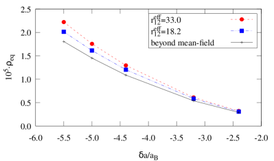
Figure 3: (Color online) Equilibrium density $\rho_{\rm eq}$ of the uniform Bose mixture as function of $\delta a$, varied by changing $a_{22}$, see table 1. For all curves, $a_{12}=-1.52$. The circles and squares are the present HNC-EL results obtained for $r_{12}^{\rm eff}=33.0$ and $18.2$, respectively. The line is the BMF result.

The density is more accessible to measurement than the energy, e.g. in Refs. Cabrera et al. (2018); Semeghini et al. (2017) the central density of droplets was measured. In Fig.3 we summarize the results shown in Fig.2 by plotting the equilibrium total density $\rho_{\rm eq}$ as a function of $\delta a$ (filled circles). Also shown in Fig.3 is the BMF result for $\rho_{\rm eq}(\delta a)$, obtained as the minimum of the real part of the BMF energy, which qualitatively agrees with HNC-EL, but predicts a somewhat lower equilibrium density. The square symbols in Fig.3 show our results for $\rho_{\rm eq}(\delta a)$, if we choose different parameters $s_{12}$ and $\sigma_{12}$ in $v_{12}(r)$ such that we keep $a_{12}=-1.519$, while changing the effective range from $r_{12}^{\rm eff}=33.0$ (upper curve) to $r_{12}^{\rm eff}=18.2$ (lower curve). This demonstrates that the results are not universal; they depend not only the $s$-wave scattering lengths, but at least also on the effective ranges.

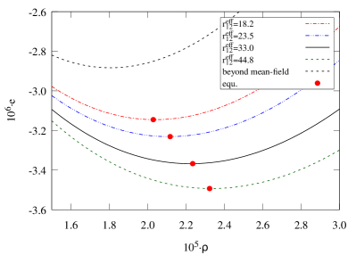
Figure 4: (Color online) $e(\rho)$ for $\delta a=-0.156$ and four models for the inter-species interaction $v_{12}$ corresponding to effective ranges $r_{12}^{\rm eff}=18.2;23.0;33.0;44.8$. Also shown is the BMF result ${\rm Re}[e_{\rm BMF}]$.

In Fig.4 shows the dependence of the energy per particle $e(\rho)$ on $r_{12}^{\rm eff}$ for $\delta a=-0.156$, with $a_{12}=-1.519$ and the other scattering lengths as above, for different values $r_{12}^{\rm eff}=18.2;23.0;33.0;44.8$. The dependence on $r_{12}^{\rm eff}$ is significant, with $e$ varying by $10\%$ and $\rho_{\rm eq}$ varying by $13\%$ for this range of $r_{12}^{\rm eff}$ values. The BMF energy ${\rm Re}[e_{\rm BMF}]$ agrees better with HNC-EL for smaller $r_{12}^{\rm eff}$. Alkali interaction potentials have a finite effective range that is often much larger than the $s$-wave scattering length, see e.g. table 1 in Ref Flambaum et al. (1999). Considering the low equilibrium densities $\rho_{\rm eq}$, it might appear surprising to find this non-universal behavior. We note, however, that for small $\delta a$ the mean-field energy is the result of large cancellations of negative and positive contributions. Therefore it is plausible that a dependence on higher-order parameters such as the effective range becomes visible.

The spinodal instability (thick black line in Fig. 1) can be relevant for the preparation of the liquid droplets, achieved by ramping one of the scattering lengths. During a fast ramp, the mixture may visit the “forbidden” region of the $(\rho_{1},\rho_{2})$-phase space and can condense into multiple droplets. To characterize the uniform liquid mixture near this instability in more detail, we choose $a_{\alpha,\beta}$ and $r_{\alpha,\beta}^{\rm eff}$ as for Fig. 1 corresponding to $\delta a=-0.156$, and the mean-field optimal ratio $\rho_{1}/\rho_{2}=1.363$. A simple approximation for the excitation spectrum of a Bose mixture is given by the Bijl-Feynman approximationFeynman (1954), which provides a good estimate of the long wave length dispersion. A mixture supports density and concentration oscillations, with dispersion relations $\epsilon_{1}(k)$ and $\epsilon_{2}(k)$, respectively. They can be easily calculated from the static structure functions $S_{\alpha\beta}(k)$ by solving the eigenvalue problem ${\hbar^{2}k^{2}\over 2m}\bm{\psi}_{i}=\epsilon_{i}(k){\bf S}(k)\bm{\psi}_{i}$ where ${\bf S}$ is the $2\times 2$ matrix with elements $S_{\alpha\beta}(k)$ and $\bm{\psi}_{i}$ are 2-component vectors. Fig. 5 shows the long-wavelength phase velocities $c_{i}=\lim_{k\to 0}d\epsilon_{i}(k)/dk$ for the density and concentration mode. The density mode has lower energy than the concentration mode for all densities shown in Fig. 5, including the equilibrium density. While $c_{2}$ is finite and hence the mixture is stable against demixing, the density mode becomes soft for $k\to 0$ as $\rho$ is lowered, evidenced by the vanishing speed of sound $c_{1}$ at the spinodal instability (vertical line), where phase separation into liquid and gas occurs. This is similar to the onset of the modulational instability in dipolar Bose gasesKadau et al. (2016b); Ferrier-Barbut et al. (2016b), which however is triggered by a vanishing roton energy with a finite wave number Ferrier-Barbut et al. (2018); Chomaz et al. (2018).

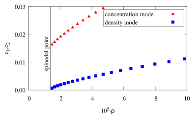
Figure 5: Long-wavelength phase velocities in the two-component Bijl-Feynman approximation for density oscillations (lower curve) and concentration oscillations (upper curve) as function of total density. The vertical line denotes the spinodal instability.

In summary, we analyze the properties of a liquid, i.e. self-bound, uniform Bose mixture using $s$-wave scattering lengths as in Refs. Cabrera et al. (2018); Semeghini et al. (2017). With the HNC-EL method, which includes pair correlations non-perturbatively, we find a narrow regime of partial densities $\rho_{\alpha}$ where the conditions for a stable liquid mixture are met: the energy per particle and both chemical potentials $\mu_{\alpha}(\rho_{1},\rho_{2})$ are negative. If $\mu_{\alpha}>0$, atoms of component $\alpha$ evaporate until reaching either equilibrium or the spinodal line. Despite their ultra-low density, the properties of these liquids depend also on the effective ranges $r_{\alpha,\beta}^{\rm eff}$. This deviation from universality was not observed in two-dimensional liquids Petrov and Astrakharchik (2016). Comparison of the energies and equilibrium densities between the BMF approximation and our HNC-EL calculations shows that the difference can probably be attributed to the neglect of the effective range in the BMF approximation. Unlike BMF energies, HNC-EL energies do not have an unphysical imaginary part for $\delta a<0$, as HNC-EL is not based on an expansion about the (unstable) mean-field result. We find that the liquid can have a spinodal instability, where the speed of sound vanishes and infinitesimal density fluctuations lead to a separation into a liquid and gas phase. This can be relevant during a nonadiabatic evolution of a droplet in experiments. In the presently available experiments Cabrera et al. (2018); Semeghini et al. (2017) the liquid droplets are far from saturation, as evidenced by the Gaussian shaped density profiles, and possibly not in equilibrium. Describing small unsaturated droplets will require an inhomogeneous generalization of HNC-EL based on the energy functional (3).

We acknowledge discussions with Leticia Tarruell and financial support by the Austrian Science Fund FWF (grant No. P23535-N20).

References

- Bloch et al. (2008) I. Bloch, J. Dalibard, and W. Zwerger, Rev. Mod. Phys. 80, 885 (2008).
- Micheli et al. (2006) A. Micheli, G. K. Brennen, and P. Zoller, Nature Physics 2, 341 (2006).
- Bloch (2005) I. Bloch, Nat. Phys. 1, 23 (2005).
- Randeria et al. (2012) M. Randeria, W. Zwerger, and M. Zwierlein, in The BCS-BEC Crossover and the Unitary Fermi Gas, Lecture Notes in Physics, Vol. 836, edited by W. Zwerger (Springer, 2012) pp. 1–32.
- Petrov (2015) D. S. Petrov, Phys. Rev. Lett. 115, 155302 (2015).
- Cabrera et al. (2018) C. R. Cabrera, L. Tanzi, J. Sanz, B. Naylor, P. Thomas, P. Cheiney, and L. Tarruell, Science 359, 301 (2018).
- Semeghini et al. (2017) G. Semeghini, G. Ferioli, L. Masi, C. Mazzinghi, L. Wolswijk, F. Minardi, M. Modugno, G. Modugno, M. Inguscio, and M. Fattori, ArXiv e-prints (2017), arXiv:1710.10890 [cond-mat.quant-gas] .
- Dalfovo et al. (1999) F. Dalfovo, S. Giorgini, L. P. Pitaevskii, and S. Stringari, Rev. Mod. Phys. 71, 463 (1999).
- Larsen (1963) D. M. Larsen, Ann. Phys. 24, 89 (1963).
- Cheiney et al. (2018) P. Cheiney, C. R. Cabrera, J. Sanz, B. Naylor, L. Tanzi, and L. Tarruell, Phys. Rev. Lett. 120, 135301 (2018).
- Kadau et al. (2016a) H. Kadau, M. Schmitt, M. Wenzel, C. Wink, T. Maier, I. Ferrier-Barbut, and T. Pfau, Nature (London) 530, 194 (2016a).
- Ferrier-Barbut et al. (2016a) I. Ferrier-Barbut, H. Kadau, M. Schmitt, M. Wenzel, and T. Pfau, Phys. Rev. Lett. 116, 215301 (2016a).
- Schmitt et al. (2016) M. Schmitt, M. Wenzel, F. Böttcher, I. Ferrier-Barbut, and T. Pfau, Nature 539, 259 (2016).
- Chomaz et al. (2016) L. Chomaz, S. Baier, D. Petter, M. J. Mark, F. Wächtler, L. Santos, and F. Ferlaino, Phys. Rev. X 6, 041039 (2016).
- Wächtler and Santos (2016) F. Wächtler and L. Santos, Phys. Rev. A 93, 061603 (2016).
- Bombin et al. (2017) R. Bombin, J. Boronat, and F. Mazzanti, Phys. Rev. Lett. 119, 250402 (2017).
- Pade (2007) J. Pade, Eur. Phys. J. D 44, 345 (2007).
- Buendia et al. (1984) E. Buendia, R. Guardiola, and M. de Llano, Phys. Rev. A 30, 941 (1984).
- Petrov and Astrakharchik (2016) D. S. Petrov and G. E. Astrakharchik, Phys. Rev. Lett. 117, 100401 (2016).
- Cikojevic et al. (2018) V. Cikojevic, K. Dzelalija, P. Stipanovic, L. Vranjes Markic, and J. Boronat, Phys. Rev. B 97, 140502 (2018).
- Chakraborty (1982) T. Chakraborty, Phys. Rev. B 26, 6131 (1982).
- Campbell (1972) C. Campbell, Annals of Physics 74, 43 (1972).
- Hebenstreit et al. (2016) M. Hebenstreit, M. Rader, and R. E. Zillich, Phys. Rev. A 93, 013611 (2016).
- Feenberg (1969) E. Feenberg, Theory of Quantum Fluids (Academic Press, 1969).
- Fabrocini and Polls (1984) A. Fabrocini and A. Polls, Phys. Rev. B 30, 1200 (1984).
- Krotscheck (1986) E. Krotscheck, Phys. Rev. B 33, 3158 (1986).
- Hansen and McDonald (1986) J. P. Hansen and I. R. McDonald, Theory of Simple Liquids (Academic Press, 1986).
- Hebenstreit (2013) M. Hebenstreit, B.S. Thesis, Johannes Kepler University, Linz (2013).
- Landau and Lifshitz (1958) L. D. Landau and E. M. Lifshitz, Quantum Mechanics (Nonrelativistic Theory), Course of Theoretical Physics, Vol. III (Pergamon Press Ltd., London - Paris, 1958).
- Pethick and Smith (2008) C. J. Pethick and H. Smith, Bose-Einstein Condensation in Dilute Gases (Cambridge University Press, 2008).
- Flambaum et al. (1999) V. V. Flambaum, G. F. Gribakin, and C. Harabati, Phys. Rev. A 59, 1998 (1999).
- Feynman (1954) R. P. Feynman, Phys. Rev. 94, 262 (1954).
- Kadau et al. (2016b) H. Kadau, M. Schmitt, M. Wenzel, C. Wink, T. Maier, I. Ferrier-Barbut, and T. Pfau, Nature 530, 194 (2016b).
- Ferrier-Barbut et al. (2016b) I. Ferrier-Barbut, H. Kadau, M. Schmitt, M. Wenzel, and T. Pfau, Phys. Rev. Lett. 116, 215301 (2016b).
- Ferrier-Barbut et al. (2018) I. Ferrier-Barbut, M. Wenzel, M. Schmitt, F. Böttcher, and T. Pfau, Phys. Rev. A 97, 011604 (2018).
- Chomaz et al. (2018) L. Chomaz, R. M. W. van Bijnen, D. Petter, G. Faraoni, S. Baier, J. Hendrik Becher, M. J. Mark, F. Wächtler, L. Santos, and F. Ferlaino, Nat. Phys (2018), doi:10.1038/s41567-018-0054-7.