Inflow Motions associated with High-mass Protostellar Objects

Abstract

We performed a molecular line survey of 82 high-mass protostellar objects in search for inflow signatures associated with high-mass star formation. Using the H¹³CO⁺ (1$-$0) line as an optically thin tracer, we detected a statistically significant excess of blue asymmetric line profiles in the HCO⁺ (1$-$0) transition, but nonsignificant excesses in the HCO⁺ (3$-$2) and H₂CO (2₁₂$-$1₁₁) transitions. The negative blue excess for the HCN (3$-$2) transition suggests that the line profiles are affected by dynamics other than inflow motion. The HCO⁺ (1$-$0) transition thus seems to be the suitable tracer of inflow motions in high-mass star-forming regions, as previously suggested. We found 27 inflow candidates that have at least one blue asymmetric profile and no red asymmetric profile, and derived the inflow velocities to be 0.23$-$2.00 km s^-1 for 20 of them using a simple two-layer radiative transfer model. Our sample is divided into two groups in different evolutionary stages. The blue excess of the group in relatively earlier evolutionary stages was estimated to be slightly higher than that of the other in the HCO⁺ (1$-$0) transition.

1 Introduction

High-mass stars (Mass $>$ 8 $M_{\odot}$, Luminosity $>$ 10³ $L_{\odot}$) have great physical and chemical importance in the interstellar environments. They affect energetics of galaxies via jets/outflows, strong radiation, and supernova explosions, and play a role in triggering next-generation star formation with the associated shocks. Furthermore, they enrich the surrounding systems and change chemical abundances. In spite of the importance of high-mass stars, there still remain questions on their formation process due to difficulties arising from observational and evolutionary limitations. In order to investigate the formation of high-mass stars, it is necessary to identify sources in different evolutionary phases, especially protostellar stage, and understand their environments.

Gravitational collapse is the most important and fundamental key process in the early stage of star formation. Unfortunately, collapsing motion is relatively harder to observe than other motions (e.g. rotation, outflow). According to the “inside-out” collapse model and observations of low-mass protostellar cores (Shu, 1977; Zhou et al., 1993; Myers et al., 1996; Evans, 1999, 2003), an asymmetric double-peaked velocity profile with higher peak at the blue-shifted part (hereafter, blue profile) can be a tool for detecting inflow signatures. The blue profile has dependences on the optical depth of the observed line and the velocity of the inflowing material. Therefore, finding adequate inflow tracers for target sources is needed to enhance our understanding. In this work, we study inflow motions toward high mass star-forming regions using several molecular transitions and try to identify suitable inflow tracers.

Although inflow motion is difficult to observe, several surveys detected statistically significant evidence of inflow motions via observations of blue profiles toward low-mass star-forming regions. The molecular line surveys with various transitions supported that active inflow motions exist regardless of the evolutionary stages of low-mass star formation (Gregersen et al., 1997, 2000; Mardones et al., 1997; Evans, 2003). Therefore, gravitational collapse is a generally accepted phenomenon for low-mass star formation both theoretically and observationally.

On the other hand, inflow studies of high-mass star-forming regions toward different samples in different inflow-tracing molecular lines show inconsistent fractions of blue asymmetries (Wu & Evans, 2003; Fuller et al., 2005; Purcell et al., 2006; Wyrowski et al., 2006; Wu07; Reiter et al., 2011; He et al., 2015; Jin et al., 2016, see Section 3.1 for detailed results). Such studies are expected to give us clues to understand the influence and importance of gravitational collapse on the formation and evolution of high-mass stars. Furthermore, they may enable us to discuss similarity between high-mass star-forming process and the low-mass counterpart. However, it is difficult not only to characterize the evolutionary stages of high-mass star-forming regions but also to find appropriate inflow tracers. Accordingly, there should be more comprehensive researches with advanced facilities toward adequate targets to understand the formation of high-mass stars.

In this study, we surveyed 82 high mass protostellar object (HMPO) candidates in multiple molecular lines by using single-dish telescopes to investigate the inflow motions via statistical analysis of the observed line spectra. We present the source selection criteria in Section 2.1 and the observational details in Section 2.2. Statistical analysis with line profiles are in Section 3.1 and identification of inflow candidates and examination of their characteristics are in Section 3.2. We discuss appropriateness of determination of profiles and statistics depending on sub-groups in Section 4. Finally, we conclude with a summary of the main results in Section 5.

2 Source selection and Observations

2.1 Source selection

In order to find potential sites of early stage of star formation, Richards et al. (1987) proposed selection criteria for identifying bright compact molecular clouds from the IRAS (InfraRed Astronomical Satellite) point source catalogue. Meanwhile, Wood & Churchwell (1989) suggested IRAS color criteria for ultracompact H II regions (UCH IIs), $[25-12]$ $\geqq$ 0.57 and $[60-12]$ $\geqq$ 1.30 . Palla et al. (1991) combined those two sets of criteria to discover bright infrared sources in the very early phases of high-mass star formation without positional coincidence with known H II regions or extragalactic objects. They found 260 $IRAS$ point sources and distinguished them into two groups. In the IRAS color-color diagram of $[25-12]$ and $[60-12]$, 125 of the 260 sources are in the region meeting the criteria of Wood & Churchwell (1989), while the remaining 135 are outside the region. They classified the 125 sources as the $\it High$ group and the 135 sources as the $\it Low$ group. Molinari et al. (1996) observed 163 among the 260 sources in the NH₃ (1, 1) and (2, 2) lines, which are believed as tracers of warm dense gas in the vicinity of embedded (proto)stars, in search for HMPO candidates. They detected NH₃ line emission in 101 sources. The detection rate of NH₃ emission is considerably higher for the $\it High$ group (80$\%$ of 80 sources) than for the $\it Low$ group (45$\%$ of 83 sources). Together with the finding of Palla et al. (1991) that the detection rate of H₂O maser emission is significantly higher in the $\it High$ group (26%) than in the $\it Low$ group (9%), this might suggest that the two groups represent different evolutionary phases of high-mass star formation, i.e., the $\it Low$ group is in an earlier evolutionary stage than the $\it High$ group (see also Molinari et al., 1998). We selected 72 of the 101 NH₃-detected sources in the catalog of Molinari et al. (1996): 47 $\it High$ and 25 $\it Low$ sources. We also added 10 $\it High$ sources from the HMPO candidate catalogs of Walsh et al. (1998, 2001), Hunter et al. (2000), and Sridharan et al. (2002). Table 1 presents the information of the 82 sources, such as the IRAS names, equatorial coordinates, kinematic distances ($d_{\rm kin}$), and infrared luminosities ($L_{\rm IR}$). We adopted the information from the original catalogs except the distances and luminosities for IRAS05391-0152 (Qin et al., 2008), IRAS06084-0611 (Gómez et al., 2002), and IRAS07427-2400 (Kumar et al., 2002).

2.2 Observations

We made single-point observations toward the 82 sources in up to five transitions, such as HCO⁺ (1$-$0), HCO⁺ (3$-$2), HCN (3$-$2), H₂CO (2₁₂$-$1₁₁) and H¹³CO⁺ (1$-$0) lines. The used telescopes were the Caltech Submillimeter Observatory (CSO) 10.4 m, the Arizona Radio Observatory (ARO) 12 m, the Submillimeter telescope (SMT) 10 m, and the Korean VLBI Network (KVN) 21 m. Table 2 summarizes the observational details, including the observed transition, frequency, telescope, main-beam size of the telescope, main-beam efficiency of the telescope, velocity resolution, and number of the observed sources.

2.2.1 CSO 10.4 m Observations

We used the CSO telescope to survey 48 sources in the HCN (3$-$2) line and 11 sources in the HCO⁺ (3$-$2) line. The observations were undertaken in 2005 October. The system temperatures ranged between 350 and 500 K. We employed the 50 MHz bandwidth acousto-optical spectrometer (AOS) with 1024 channels as the backend and obtained typical rms noise levels ($T_{\rm A}^{*}$) of 0.17 K and 0.27 K at a velocity resolution of 0.22 km s^-1 after smoothing for HCN (3$-$2) and HCO⁺ (3$-$2), respectively.

2.2.2 ARO 12 m and SMT Observations

We surveyed 60, 52, and 45 sources in the HCO⁺ (1$-$0), H₂CO (2₁₂$-$1₁₁), and H¹³CO⁺ (1$-$0) lines, respectively, using the previous generation 12 m telescope. The backends were filterbanks with 256 channels and a bandwidth of 25.6 MHz (100 kHz resolution) each. The system temperatures were around 350 K at $\sim$89 GHz and 400 K at 140 GHz. The receivers were dual polarization, single-sideband SIS systems where the image rejection was typically 20 dB, obtained by tuning the mixer backshort. The observed temperatures were obtained on the $T_{\rm R}^{*}$ scale (Mangum, 2000). The rms noise levels were 0.07 K at $\sim$0.34 km s^-1 resolution and 0.08 K at 0.21 km s^-1 resolution for $\sim$89 and 140 GHz, respectively.

We also surveyed 32 sources in the HCO⁺ (3$-$2) line using the SMT. The 64 MHz filterbanks with 256 channels were used with a spectral resolution of 250 kHz. The system temperatures were around 900 K. The single polarization receiver in this case utilized the ALMA Band 6 sideband-separating SIS mixers. The observed temperatures were obtained on the $T_{\rm A}^{*}$ scale. The rms noise level was 0.12 K at a resolution of 0.28 km s^-1. These observations were all conducted in 2006 June.

2.2.3 KVN 21 m Observations

We observed 14, 19, and 30 sources in the HCO⁺ (1$-$0), H₂CO (2₁₂$-$1₁₁), and H¹³CO⁺ (1$-$0) lines, respectively, using the KVN 21 m telescopes at the Yonsei and Tamna stations (Kim et al., 2011). The observations were performed in 2014 May and June, 2015 February, and 2016 June. The system temperatures usually ranged between 200 and 300 K. The backends were the digital spectrometers with 4096 channels and a bandwidth of 64 MHz each. The noise levels ($T_{\rm A}^{*}$) were typically 0.04, 0.06, and 0.02 K at velocity resolutions of 0.21, 0.27, and 0.22 km s^-1 after smoothing for the HCO⁺ (1$-$0), H₂CO (2₁₂$-$1₁₁), and H¹³CO⁺ (1$-$0) transitions, respectively, with two exceptions. The velocity resolution was 0.43 km s^-1 for IRAS05137+3919 and IRAS05345+3157 in the H¹³CO⁺ (1$-$0).

3 Results

3.1 Line Asymmetries

Mardones et al. (1997) proposed a dimensionless parameter $\delta v$ to quantify asymmetry of the observed optically thick line profiles : $\delta v=(v_{thick}-v_{thin})/\vartriangle\!\!v_{thin}$. Here $v_{thin}$ and $v_{thick}$ are the peak velocities of the optically thin and thick lines, respectively, and $\vartriangle\!\!v_{thin}$ is the full width at half maximum (FWHM) of the optically thin line. This parameter has been generally used in previous inflow studies of low- and high-mass star-forming regions. The $v_{thick}$ is directly obtained from the observed profile while $v_{thin}$ and $\vartriangle\!\!v_{thin}$ are measured by Gaussian fitting to the observed profile. The optically thin line used in this study is the H¹³CO⁺ (1$-$0) line. Table 3 presents the determined parameters for the optically thin and thick lines. In order to confirm that H¹³CO⁺ (1$-$0) line emission is optically thin, we derived the peak optical depth, $\tau_{thin}$, using the following equations:

$$\tau_{thin}=-\ln\biggl{[}1-\frac{T_{thin}}{(T_{ex}-J_{\nu}(T_{bg}))}\biggr{]},$$ (1)

and

$$J_{\nu}(T)=\frac{h\nu}{k}\frac{1}{(e^{h\nu/kT}-1)}.$$ (2)

Here T_thin is the brightness temperature of the optically thin line, H¹³CO⁺ (1$-$0)  in this work, and T_bg is the background brightness temperature, which is assumed as 2.73 K. We assumed that the HCO⁺ (1$-$0) line is optically thick (1$-$ e^-τ $\approx$ 1) and that both HCO⁺ (1$-$0) and H¹³CO⁺ (1$-$0) lines arise from the same volume with the same excitation temperature, T_ex. The excitation temperature can be calculated from the equation

$$T_{ex}=\frac{h\nu}{k}\biggl{[}\ln\biggl{(}1+\frac{(h\nu/k)}{T_{thick}+J_{\nu}(T_{bg})}\biggr{)}\biggr{]}^{-1},$$ (3)

where T_thick is the brightness temperature of the optically thick line, HCO⁺ (1$-$0). Table 3 lists the estimated optical depths of the H¹³CO⁺ (1$-$0) line emission in the second column. The values range from 0.04 to 0.36, with an average value of 0.13. Thus the H¹³CO⁺ (1$-$0) line emission seems to be optically thin enough to measure the systemic velocity and the velocity dispersion of the target clumps. The above assumption of same emitting volume and excitation temperature for the HCO⁺ and H¹³CO⁺ lines may be questionable because of different optical depths. That makes the two lines trace different depths of the clump and hence different volumes. However, the H¹³CO⁺ line seems to be practically the best choice because other molecular lines might trace more different volumes.

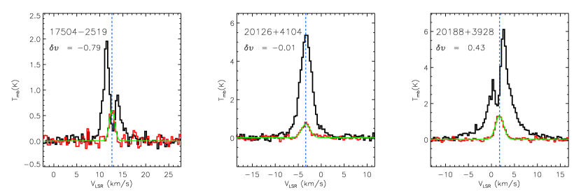
Figure 1: Spectra for representative B profiles (left), N profiles (middle) and R profiles (right). In each panel, the red and black solid lines show the HCO⁺ (1–0) and H¹³CO⁺ (1–0) line profiles, respectively. The blue-dotted vertical line indicates the peak velocity of the H¹³CO⁺ (1–0) line from the gaussian fitting result in green. The IRAS name and the estimated $\delta v$ are presented at the top left corner (Table 3).

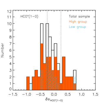
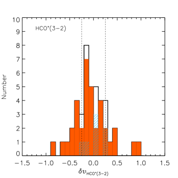
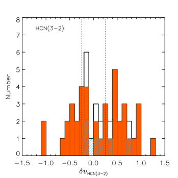
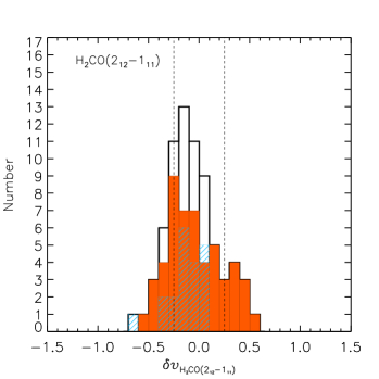
Figure 2: Histograms of $\delta v$ for the observed optically thick lines: HCO⁺ (1–0), HCO⁺ (3–2), HCN (3–2), and H₂CO (2₁₂–1₁₁). The black solid lines are for the entire sample, while the orange-colored bars and the cyan hatched bars are for the $\it High$ and $\it Low$ groups, respectively. The vertical dotted lines indicate the threshold values of $\delta v$, $\pm$0.25.

As in most previous inflow studies (e.g. Mardones et al., 1997; Gregersen et al., 1997; Fuller et al., 2005), we categorized the optically thick line profiles into three types on the basis of the measured value of $\delta v$: blue (B) for $\delta v<-0.25$, red (R) for $\delta v>0.25$, neither (N) for $-0.25\leq\delta v\leq 0.25$. Figure 1 displays sample HCO⁺ (1$-$0) spectra with B, N, and R profiles along with the H¹³CO⁺ (1$-$0) spectra. We counted the numbers of B, R, and N profiles ($N_{Blue}$, $N_{Red}$, $N_{Neither}$, and N${}_{Total}\equiv N_{Blue}$+$N_{Red}$+$N_{Neither}$) for each optically thick line. The detection rates of blue profiles D_Blue (=N_Blue/N_Total) are 0.39, 0.26, 0.25 and 0.25, and those of red profiles D_Red (=N_Red/N_Total) are 0.19, 0.16, 0.40 and 0.13 in the HCO⁺ (1$-$0), HCO⁺ (3$-$2), HCN (3$-$2), and H₂CO (2₁₂$-$1₁₁) lines, respectively (Table 4). Table 3 presents the estimated values of $\delta v$ and identified profile types for each source in the individual optically thick lines, and Figure 2 exhibits histograms of $\delta v$ for each transition.

We are able to quantify the dominance of blue profile with respect to red profile by the non-dimensional parameter, so-called blue excess (E), introduced by Mardones et al. (1997) :

$$E=(N_{Blue}-N_{Red})/N_{Total}.$$ (4)

Table 4 summarizes our statistical analysis results in four optically thick molecular lines. As mentioned above, the H¹³CO⁺ (1$-$0) line is used as an optically thin tracer to determine $v_{thin}$ and $\vartriangle\!\!v_{thin}$. We found 29 blue profiles and 14 red profiles in the HCO⁺ (1$-$0) line for a sample of 74 sources. The blue excess E for the HCO⁺ (1$-$0) line is 0.20. This value is in good agreement with the estimate (E=0.22) obtained by He et al. (2015) for 201 HMPOs in the same transition, and is slightly higher than the estimates of E=0.15 acquired by Fuller et al. (2005) for 68 HMPOs and E=0.17 by Wu07 for 29 HMPOs. We found less significant blue excesses of E=0.09 and E=0.13 in the HCO⁺ (3$-$2) and H₂CO (2₁₂$-$1₁₁) lines, respectively. For comparison, Fuller et al. (2005) obtained E=0.04 in the HCO⁺ (3$-$2) for 24 sources and E=0.19 in the H₂CO (2₁₂$-$1₁₁) for 64 sources. On the other hand, we found 12 blue and 19 red profiles in the HCN (3$-$2) line for 48 sources. Thus, our sample shows a quite significant red excess of E=–0.15, suggesting that the HCN (3$-$2) line traces other dynamics rather than inflows in HMPOs, such as outflow, rotation, and turbulent motions. In contrast, Wu & Evans (2003) measured a blue excess of 0.21 in the HCN (3$-$2) for 28 UCHIIs and compact HII regions, which are mostly more evolved and luminous than the sources in our sample (see Section 4). The molecular tracer appears to have suitable optical depth and critical density for their sample but this is not the case for most sources in our sample.

In order to get rid of the statistical uncertainty coming from the use of different beam sizes of the telescopes, we also obtained statistics of line parameters separately for the ARO 12 m and the KVN 21 m. That is, we calculated blue excesses of the HCO⁺ (1$-$0) line using the H¹³CO⁺ (1$-$0) line as an optically thin line observed by the same telescope. In case of the ARO 12 m, the numbers of blue and red profiles are 19 and 9, respectively, out of total 45 sources, which leads to blue excess of E=0.22. On the other hand, in case of the KVN 21 m, the numbers of blue and red profiles are 5 and 2, respectively, for total 14 sources, which leads to blue excess of E=0.21. However, the blue excess of the latter case has statistical weakness arising from the small number of sources. If we combine two observations, the numbers of blue and red profiles are 24 and 11, respectively, for total 59 sources and hence the blue excess is E=0.22. Thus our statistics for the entire 74 sample (E=0.20) obtained by the combination of the HCO⁺ (1$-$0) and H¹³CO⁺ (1$-$0) lines detected by different telescopes seems to be acceptable.

To evaluate the probability that the measured blue excess is produced by coincidence from a random distribution with the same numbers of blue and red profiles, we performed a binomial test (Fuller et al., 2005; Wu07; He et al., 2015; Jin et al., 2016) defined as

$$P(X\geq V)=\sum_{x=V}^{N}\frac{N!}{x!(N-x)!}p^{x}(1-p)^{(N-x)}.$$ (5)

Here, $N$ is the number of performances, $V$ is the the number of successes, and $p$ is the probability of occurrence in a single independent performance. In our case, $N$ is the total number of blue and red profiles and $V$ is the number of blue profiles. Table 4 also lists the derived values of $P$. The $P$ value for the HCO⁺(1–0) line is 0.016, which implies that the estimated blue excess (E=0.20) is very unlikely to be generated by chance from an even distribution.

3.2 Inflow candidates

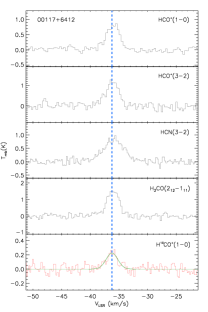
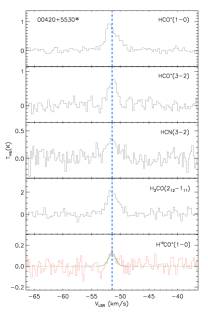
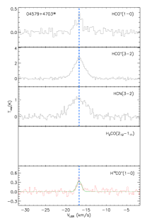
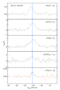
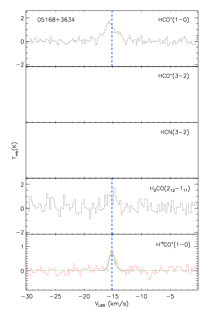
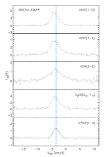
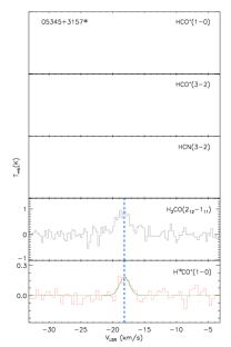
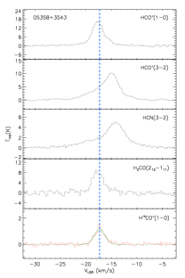
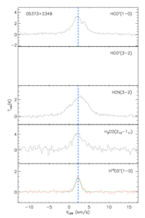
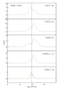
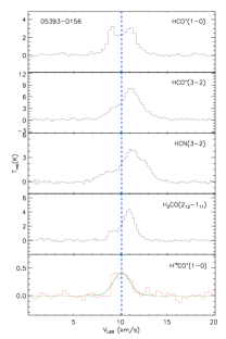
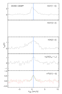
Figure A1: Detected molecular line spectra of the individual sources. For each source, the IRAS name is presented at the upper left corner in the top panel and the transition is listed at the upper right corner in each panel. The vertical blue dotted line is the central velocity of the H¹³CO⁺ (1$-$0) line determined by Gaussian fitting. The line spectrum is displayed in red with the Gaussian fitting result in green in the bottom panel. The inflow candidates are marked with asterisks on the source names. The empty panel means that the transition was not observed for a given source.

Since the sources in our sample were observed in multiple optically thick lines, one source can be classified as different profile types in different transitions. We thus identified strong inflow candidates as in some previous studies using the two criteria: 1) at least one blue (B) profile and 2) no red (R) profile (e.g. Mardones et al., 1997; Fuller et al., 2005). There are 27 sources satisfying the criteria. The inflow candidates are marked with asterisks in the first column of Table 3 (see also Figure A1). Three of them (IRAS05490+2658, IRAS19282+1814, IRAS23545+6508) had been observed by Fuller et al. (2005) as well, but only IRAS05490+2658 was identified as an inflow candidate while the other two did not show any line asymmetry (see their Table 9). In reality, their observed positions are offset from ours by 12^′′, 76^′′, and 23^′′ for IRAS05490+2658, IRAS19282+1814, and IRAS23545+6508, respectively. The large offsets can cause the non-detection of blue asymmetry in their line profiles of HCO⁺ (1$-$0) and H₂CO (2₁₂$-$1₁₁) for IRAS19282+1814 and IRAS23545+6508, taking into account their beam sizes of 29^′′ at 89 GHz and 17^′′ at 140 GHz. Therefore, all the 27 sources but IRAS05490+2658 are newly identified inflow candidates. It should be noted that the HCN (3$-$2) spectrum of IRAS04579+4703 and the H₂CO (2₁₂$-$1₁₁) spectrum of IRAS05345+3157 are quite noisy (Fig. A1) and so their classifications as blue profiles need to be confirmed by more sensitive observations.

We derived the inflow velocities, $v_{in}$, for 20 inflow candidates with blue HCO⁺ (1$-$0) line profiles using the two-layer radiative transfer model of Myers et al. (1996). The model assumes two uniform layers approaching toward each other with different excitation temperatures. The inflow velocity is determined by both optical depth and excitation temperature. The estimated inflow velocities range from 0.23 to 2.00 km s^-1 with a median value of 0.49 km s^-1 (Table 3). These values are comparable to the estimates (0.1$-$1.8 km s^-1) of Klaassen & Wilson (2007) for 8 high-mass star-forming clumps. For further detailed studies, including measurements of the inflow region size and the inflow mass rate, the mapping observations of the blue profiles are required.

On the other hand, we also found 18 sources that have at least one red profile and no blue profile. It is likely that the profiles might be affected by dynamics other than inflow motion. There are 12 sources with both blue and red profiles. They are all classified as $High$ sources, and 7 of them show blue profiles in the HCO⁺ (1$-$0) transition but red profiles in the HCN (3$-$2) transition.

4 Discussion

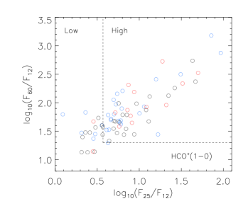
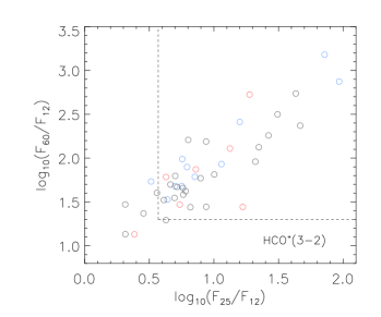
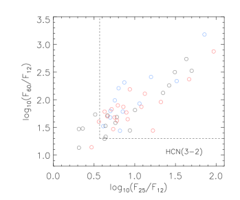
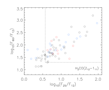
Figure 3: $IRAS$ Color-color diagrams of [25-12] vs. [60-12] for the optically thick lines. The dotted lines are the IRAS color criteria of Wood & Churchwell (1989) for UCH II candidates ($High$ sources), $[25-12]$ $\geqq$ 0.57 and $[60-12]$ $\geqq$ 1.30. The blue, red, and black open circles represent blue, red, and neutral profiles in each line, respectively.

Our sample is divided into two groups ($\it Low$ and $\it High$) in the IRAS color-color diagram of $[25-12]$ and $[60-12]$, as discussed in Section 2.1. The sources in the $High$ group are believed to be in relatively more evolved stage than those of the $Low$ group, although the two groups have similar distributions of infrared luminosities (Palla et al., 1991; Molinari et al., 1996, 1998). We derive blue excesses separately for the $Low$ and $High$ groups. Table 5 presents the statistical results in all the optically thick transitions (see also Figure 2) and Figure 3 shows the distributions of blue- and red-profile sources in the two groups on the color-color diagram. In comparison with the $\it High$ group, the $\it Low$ group shows higher blue excesses in the HCO⁺ (1$-$0) and H₂CO (2₁₂$-$1₁₁) lines but lower excesses in the HCO⁺ (3$-$2) and HCN (3$-$2) lines. In case of the $\it Low$ group, however, it should be noted that only the HCO⁺ (1$-$0) and H₂CO (2₁₂$-$1₁₁) lines have statistically sufficient numbers of sources and so the blue excess estimates of the HCO⁺ (3$-$2) and HCN (3$-$2) lines may not be meaningful. Thus, further observations for substantially large number of sources are required for the latter transitions to obtain more significant results for evolutionary study of inflow.

There are very few previous studies investigating the evolutionary effect in the inflow statistics, the results of which are inconclusive. Wu07 reported a higher blue excess for 12 UCHIIs (E=0.58) than 29 HMPOs (E=0.17) in the HCO⁺ (1$-$0) transition. Jin et al. (2016) also found a similar increasing trend in the HCN (1-0) line for their sample consisting of 26 HMPOs (E=0.15) and 23 UCHIIs (E=0.30), although they obtained the highest blue excess (E=0.42) for 12 high-mass prestellar clumps. On the contrary, He et al. (2015) found a decreasing evolutionary trend of blue excess in the HCO⁺ (1$-$0) line for a much larger sample: E=0.29 for 84 prestellar clumps, 0.22 for 201 HMPOs, –0.11 for 79 UCHIIs. Our result is consistent with that of He et al. (2015) although the decreasing trend is less prominent. This difference may be because their sample contains many more evolved UCHIIs than $\it High$ sources in our sample.

Fuller et al. (2005) surveyed 77 submillimeter clumps associated with HMPOs in multiple molecular lines for an extensive inflow study toward high-mass star-forming regions. The blue excesses were derived to be E=0.15 and E=0.19 for the HCO⁺ (1$-$0) and H₂CO (2₁₂$-$1₁₁) lines, respectively. When they considered only sources with distances $\leq$6 kpc in order to avoid beam dilution effect due to large distances of the sources, the excesses considerably increased and became comparable to the values estimated for low-mass star-forming regions, E $\simeq$ 0.3 (Evans, 2003). However, we do $not$ find such trend in the same analysis for our sample. For instance, the blue excesses for the HCO⁺ (1$-$0) and H₂CO (2₁₂$-$1₁₁) lines are E=0.20 and E=0.13 for the entire sample and E=0.12 and E=0.16 for the 65 and 63 sources within 6 kpc, respectively. This inconsistent result may be caused by large uncertainty in the determination of the distances to the sources. The vast majority of the sources in both samples of ours and Fuller et al. (2005) are located in the inner Galaxy, but the distance ambiguity is $not$ resolved for most of them.

As noted in Section 3.1, Wu & Evans (2003) found that the HCN (3$-$2) line shows a significant blue excess (E=0.21) for their sample and thus it is useful for tracing inflow motions toward UCHIIs and compact HII regions. However, we find that the transition is much worse tracer of inflow motions toward HMPOs in our sample than the HCO⁺ (1$-$0) line. It is worthwhile to note that their sources are more massive and luminous as well as more evolved than ours, median mass of 8.9$\times$10² M_⊙ & median $L_{\rm IR}$ of 1.06$\times$10⁵ L_⊙ (Wu & Evans, 2003) vs. median $L_{\rm IR}$ of 1.11$\times$10⁴ L_⊙. In fact, the critical density of the HCN (3$-$2) transition is two orders of magnitude larger than that of the HCO⁺ (1$-$0) transition (Shirley, 2015). Therefore, we interpret that the HCO⁺ (1$-$0) line, which has relatively low critical density, is better suited for investigating inflow motions in our sources than the HCN (3$-$2) line. This seems to be consistent with the previous suggestion that the characteristic blue profile will show up only if the critical density of the molecular tracer is suitable for optical depth of the target (Myers et al., 1996; Wu & Evans, 2003).

Although the blue profile has been widely accepted as an evidence of infall motions, as noted earlier, it is sometimes tricky to interpret the signature due to other kinematics, especially for massive star-forming regions that are much more turbulent and distant than low-mass star-forming regions. Alternatively, the red-shifted absorption feature can be used to study inflow motions in massive star-forming regions because they are usually bright radio and infrared sources. For example, Wyrowski et al. (2012, 2016) observed 11 massive molecular clumps in the NH₃ 3₂₊–2_2- line at 1.81 THz using the GREAT instrument onboard SOFIA (beam size = 16^′′). They detected red-shifted NH₃ absorption features with respect to the systemic velocities toward 8 sources, and derived the velocity shifts to be 0.3–2.9 km s^-1. Thier measurements are roughly in agreement with the estimated infall velocities of this study (see Section 3.2). These two kinds of studies utilizing blue profiles and red-shifted absorption features would complement each other.

5 Conclusions and Summary

We performed a survey of one optically thin and up to four optically thick molecular lines toward 82 HMPO candidates to understand gravitational collapse in the early stage of high-mass star formation. To quantify asymmetries of the optically thick line profiles, we derived $\delta v$’s of the individual sources in each transition and estimated the blue excess for our sample with $\delta v$=$\pm$0.25 as threshold values. The main results are summarized as follows.

1. We obtained a statistically significant blue excess in the HCO⁺ (1$-$0) line (E=0.20), but non-significant excesses in the HCO⁺ (3$-$2) and the H₂CO (2₁₂$-$1₁₁) lines (E=0.09 and E=0.13, respectively). The HCN (3$-$2) line shows a negative blue excess of E=$-$0.15. The HCO⁺ (1$-$0) line thus seems to be the suitable tracer of inflow motions in high-mass star-forming regions as some previous studies proposed (e.g. Fuller et al., 2005; Wu07). On the contrary, the other lines do not appear to have suitable opacity and critical density for the appearance of blue profile toward most sources in our sample, and may be affected by dynamics other than inflow, such as outflow, rotation, turbulent motions.

2. We found 27 inflow candidates by adopting the criteria of Fuller et al. (2005), namely, one or more blue profiles and no red profile. All of them are newly identified inflow candidates except one (IRAS05490+2658), which had been classified by Fuller et al. (2005) as an inflow candidate. We derived inflow velocities for 20 out of the 27 candidates using the two-layer radiative transfer model of Myers et al. (1996). The estimated inflow velocities range between 0.23 and 2.00 km s^-1 with a median value of 0.49 km s^-1. On the other hand, there are 18 sources that have red profile(s) but no blue profile. They might be more affected by dynamics other than inflow motion in the observed optically thick lines.

3. The sources in our sample are all HMPO candidates but they are known to be divided into two different evolutionary stages: $\it Low$ and $\it High$ groups. The statistical results for the $\it Low$ group show that blue excesses in the HCO⁺ (1$-$0) and H₂CO (2₁₂$-$1₁₁) lines, of which the number of both groups are statistically meaningful, are slightly higher than those for $\it High$ groups. We also estimated blue excesses for a subsample of sources at relatively small ($\leq$6 kpc) distances and obtained less significant excesses than those for the entire sample. This is not consistent with the result of Fuller et al. (2005). This discrepancy may be caused by large uncertainties in determining the distances to the sources in our and their samples.

Table 1: Source Information

IRAS	R.A.	Decl.	$d_{\rm kin}$	$L_{\rm IR}$
Name	(J2000)	(J2000)	(kpc)	($L_{\odot}$)	Group
$00117+6412$	00 14 27.7	+64 28 46	1.80	1.38E+03	H
$00420+5530$	00 44 57.6	+55 47 18	7.72	5.15E+04	L
$04579+4703$	05 01 39.7	+47 07 23	2.47	3.91E+03	H
$05137+3919$	05 17 13.3	+39 22 23	10.8	5.61E+04	L
$05168+3634$	05 20 16.2	+36 37 21	6.08	2.40E+04	H
$05274+3345$	05 30 45.6	+33 47 52	1.55	4.53E+03	H
$05345+3157$	05 37 47.8	+31 59 24	1.80	1.38E+03	L
$05358+3543$	05 39 10.4	+35 45 19	1.80	6.31E+03	H
$05373+2349$	05 40 24.4	+23 50 54	1.17	6.64E+02	L
$05391-0152$	05 41 38.7	-01 51 19	0.50	1.96E+03	H
$05393-0156$	05 41 49.5	-01 55 17	0.50	1.10E+04	H
$05490+2658$	05 52 13.0	+26 59 34	2.10	3.16E+03	H
$05553+1631$	05 58 13.9	+16 32 00	3.04	1.17E+04	H
$06053-0622$	06 07 46.7	-06 23 00	0.80	2.90E+04	H
$06056+2131$	06 08 41.0	+21 31 01	1.50	5.83E+03	H
$06061+2151$	06 09 07.8	+21 50 39	0.10	2.78E+01	H
$06084-0611$	06 10 51.0	-06 11 54	1.00	9.60E+03	H
$06103+1523$	06 13 15.1	+15 22 36	4.63	1.91E+04	H
$06105+1756$	06 13 28.3	+17 55 33	3.38	1.60E+04	H
$06382+0939$	06 41 02.7	+09 36 10	0.76	1.63E+02	L
$06584-0852$	07 00 51.5	-08 56 29	4.48	9.08E+03	L
$07299-1651$	07 32 10.0	-16 58 15	1.40	6.30E+03	H
$07427-2400$	07 44 51.9	-24 07 41	6.40	5.00E+04	H
$17417-2851$	17 44 53.4	-28 52 20	0.10	3.17E+01	H
$17450-2742$	17 48 09.3	-27 43 21	0.10	1.57E+01	L
$17504-2519$	17 53 35.2	-25 19 56	3.65	9.32E+03	H
$17527-2439$	17 55 49.1	-24 40 20	3.23	1.53E+04	H
$18014-2428$	18 04 29.3	-24 28 47	2.87	1.71E+04	L
$18018-2426$	18 04 53.9	-24 26 41	1.50	6.64E+03	L
$18024-2119$	18 05 25.4	-21 19 41	0.12	1.08E+01	L
$18089-1732$	18 11 51.3	-17 31 28	3.48	6.33E+04	H
$18134-1942$	18 16 22.3	-19 41 20	1.62	7.62E+03	H
$18144-1723$	18 17 24.4	-17 22 13	4.33	1.32E+04	L
$18151-1208$	18 17 57.1	-12 07 22	3.04	3.32E+04	H
$18159-1550$	18 18 47.6	-15 48 54	4.66	3.10E+04	H
$18159-1648$	18 18 53.5	-16 47 39	2.50	2.95E+04	H
$18162-1612$	18 19 07.5	-16 11 21	4.89	2.94E+04	L
$18236-1205$	18 26 24.3	-12 03 47	2.51	1.04E+04	H
$18256-0742$	18 28 20.5	-07 40 22	2.90	1.11E+04	L
$18258-0737$	18 28 34.1	-07 35 31	2.97	3.31E+04	H
$18316-0602$	18 34 19.8	-05 59 44	3.17	4.14E+04	H
$18317-0513$	18 34 25.9	-05 10 59	3.13	3.48E+04	H
$18360-0537$	18 38 40.3	-05 35 06	6.28	1.16E+05	H
$18372-0541$	18 39 56.0	-05 38 49	1.87	7.18E+03	H
$18396-0431$	18 42 18.8	-04 28 37	6.08	4.23E+04	L
$18488+0000$	18 51 24.8	+00 04 19	5.48	5.14E+04	H
$18507+0121$	18 53 17.4	+01 24 55	3.87	4.84E+04	H
$18511+0146$	18 53 38.1	+01 50 27	3.86	2.01E+04	L
$18527+0301$	18 55 16.5	+03 05 07	5.26	1.63E+04	L
$18532+0047$	18 55 50.6	+00 51 22	3.96	1.27E+04	H
$18565+0349$	18 59 03.4	+03 53 22	6.77	2.62E+04	L
$18566+0408$	18 59 09.9	+04 12 14	6.76	1.02E+05	H
$18567+0700$	18 59 13.6	+07 04 47	2.16	8.39E+03	L
$19045+0518$	19 06 59.3	+05 22 55	3.80	1.09E+04	H
$19088+0902$	19 11 15.9	+09 07 27	4.71	2.99E+04	H
$19282+1814$	19 30 28.1	+18 20 53	2.11	1.63E+04	H
$19368+2239$	19 38 58.1	+22 46 32	4.44	8.63E+03	H
$20050+2720$	20 07 06.7	+27 28 53	0.73	3.88E+02	H
$20056+3350$	20 07 31.5	+33 59 39	1.67	4.00E+03	H
$20062+3550$	20 08 09.8	+35 59 20	0.08	5.40E+00	H
$20106+3545$	20 12 31.3	+35 54 46	1.64	1.79E+03	L
$20126+4104$	20 14 26.0	+41 13 32	4.18	7.12E+04	H
$20188+3928$	20 20 39.3	+39 37 52	0.31	3.43E+02	H
$20220+3728$	20 23 55.7	+37 38 10	4.49	8.09E+04	H
$20227+4154$	20 24 31.4	+42 04 17	0.10	9.14E+00	H
$20278+3521$	20 29 46.9	+35 31 39	5.02	1.08E+04	L
$20286+4105$	20 30 27.9	+41 15 48	3.72	3.90E+04	H
$20333+4102$	20 35 09.5	+41 13 18	0.10	4.57E+01	L
$21078+5211$	21 09 25.2	+52 23 44	1.49	1.34E+04	H
$21391+5802$	21 40 42.4	+58 16 10	0.75	9.39E+01	H
$21519+5613$	21 53 39.2	+56 27 46	7.30	1.91E+04	H
$22172+5549$	22 19 09.0	+56 04 45	2.87	4.78E+03	L
$22198+6336$	22 21 27.6	+63 51 42	1.28	1.24E+03	H
$22267+6244$	22 28 29.3	+62 59 44	0.45	1.10E+02	H
$22272+6358$	22 28 52.2	+64 13 44	1.23	1.97E+03	H
$22308+5812$	22 32 46.1	+58 28 22	3.70	2.09E+04	H
$22506+5944$	22 52 38.6	+60 00 56	5.70	2.22E+04	H
$23026+5948$	23 04 45.7	+60 04 35	5.76	1.76E+04	L
$23133+6050$	23 15 31.5	+61 07 08	5.20	1.20E+05	H
$23140+6121$	23 16 11.7	+61 37 45	6.44	4.35E+04	L
$23314+6033$	23 33 44.4	+60 50 30	2.78	1.09E+04	L
$23545+6508$	23 57 05.2	+65 25 11	1.27	3.89E+03	H

Table 2: Summary of the Observations

Observed	Frequency		$\theta_{\rm mb}$		$\vartriangle\!\!v$	Number
Transition	(GHz)	Telescope	(′′)	$\eta_{mb}$	(km s-1)	of Sources
HCO+ (1$-$0)	89.188526	ARO 12 m	70	0.95a	0.34	60
		KVN 21 m	32	0.38	0.21	14
HCO+ (3$-$2)	267.557633	CSO 10.4 m	27	0.61	0.22	11
		SMT 10 m	28	0.78	0.28	32
HCN (3$-$2)	265.886431	CSO 10.4 m	27	0.61	0.22	48
H2CO (212$-$111)	140.839515	ARO 12 m	44	0.80a	0.21	52
		KVN 21 m	24	0.27	0.27	19
H13CO+ (1$-$0)	86.754330	ARO 12 m	72	0.95a	0.35	45
		KVN 21 m	32	0.38	0.22	30

Table 3: Line Velocities and Asymmetry Parameters

IRAS	H13CO+ (1–0)				$v_{thick}$a					$\delta v$					Profile
Name	$\tau_{\rm thin}$b	$v$ $(v_{\rm err})$a	$\vartriangle\!\!v$ ($\vartriangle\!\!v_{\rm err}$)a		L1c	L2c	L3c	L4c		L1	L2	L3	L4		L1	L2	L3	L4		$v_{\rm in}^{a}$
$00117+6412$	0.09	-36.21 ( 0.11 )	2.32 ( 0.30 )		-35.46	-36.44	-35.63	-36.20		0.32	-0.10	0.25	0.00		R	N	N	N		$\cdots$
$00420+5530^{*}$	0.05	-51.44 ( 0.21 )	1.41 ( 0.55 )		-52.04	-51.34	-51.71	-51.80		-0.43	0.07	-0.20	-0.26		B	N	N	B		0.50
$04579+4703^{*}$	0.18	-16.70 ( 0.08 )	1.43 ( 0.20 )		-16.67	-16.55	-17.32	$\cdots$		0.02	0.11	-0.44	$\cdots$		N	N	B	$\cdots$		$\cdots$
$05137+3919^{*}$	0.05	-25.32 ( 0.16 )	1.46 ( 0.31 )		-26.58	-25.20	-25.28	-25.27		-0.86	0.08	0.03	0.04		B	N	N	N		0.35
$05168+3634$	0.24	-15.15 ( 0.06 )	1.18 ( 0.18 )		-15.68	$\cdots$	$\cdots$	-14.73		-0.45	$\cdots$	$\cdots$	0.36		B	$\cdots$	$\cdots$	R		$\cdots$
$05274+3345^{*}$	0.21	-3.36 ( 0.04 )	2.49 ( 0.08 )		-4.47	-3.77	-3.63	-4.00		-0.45	-0.16	-0.11	-0.26		B	N	N	B		0.48
$05345+3157^{*}$	$\cdots$	-18.16 ( 0.17 )	1.99 ( 0.33 )		$\cdots$	$\cdots$	$\cdots$	-18.80		$\cdots$	$\cdots$	$\cdots$	-0.32		$\cdots$	$\cdots$	$\cdots$	B		$\cdots$
$05358+3543$	0.07	-17.31 ( 0.04 )	2.38 ( 0.10 )		-17.84	-14.96	-14.21	-18.00		-0.22	0.99	1.30	-0.29		N	R	R	B		$\cdots$
$05373+2349$	0.32	2.23 ( 0.03 )	1.66 ( 0.08 )		1.95	$\cdots$	2.79	2.00		-0.17	$\cdots$	0.34	-0.14		N	$\cdots$	R	N		$\cdots$
$05391-0152$	0.16	9.91 ( 0.04 )	1.21 ( 0.10 )		9.16	10.89	11.03	10.53		-0.62	0.81	0.93	0.52		B	R	R	R		$\cdots$
$05393-0156$	0.09	10.13 ( 0.07 )	2.06 ( 0.16 )		9.16	11.10	11.03	10.96		-0.47	0.47	0.44	0.40		B	R	R	R		$\cdots$
$05490+2658^{*}$	0.13	0.55 ( 0.07 )	1.24 ( 0.19 )		0.11	$\cdots$	0.33	0.73		-0.36	$\cdots$	-0.18	0.15		B	$\cdots$	N	N		0.50
$05553+1631$	0.12	5.65 ( 0.05 )	1.90 ( 0.12 )		6.37	$\cdots$	5.29	5.47		0.38	$\cdots$	-0.19	-0.10		R	$\cdots$	N	N		$\cdots$
$06053-0622$	0.07	10.49 ( 0.08 )	2.64 ( 0.22 )		9.83	10.45	10.59	9.89		-0.25	-0.01	0.04	-0.23		N	N	N	N		$\cdots$
$06056+2131$	0.10	2.54 ( 0.03 )	2.22 ( 0.06 )		2.53	2.81	$\cdots$	2.73		0.00	0.12	$\cdots$	0.09		N	N	$\cdots$	N		$\cdots$
$06061+2151$	0.13	-0.88 ( 0.08 )	2.02 ( 0.19 )		-1.05	$\cdots$	-0.02	-1.00		-0.08	$\cdots$	0.43	-0.06		N	$\cdots$	R	N		$\cdots$
$06084-0611$	0.13	11.59 ( 0.06 )	1.98 ( 0.14 )		11.85	11.10	11.25	11.60		0.13	-0.25	-0.17	0.00		N	N	N	N		$\cdots$
$06103+1523$	0.09	15.57 ( 0.05 )	1.87 ( 0.11 )		16.37	$\cdots$	16.76	16.27		0.43	$\cdots$	0.64	0.37		R	$\cdots$	R	R		$\cdots$
$06105+1756^{*}$	0.04	7.78 ( 0.14 )	1.32 ( 0.36 )		7.24	$\cdots$	7.46	$\cdots$		-0.41	$\cdots$	-0.24	$\cdots$		B	$\cdots$	N	$\cdots$		0.28
$06382+0939$	0.33	5.22 ( 0.02 )	2.13 ( 0.06 )		4.70	$\cdots$	4.94	5.31		-0.24	$\cdots$	-0.13	0.04		N	$\cdots$	N	N		$\cdots$
$06584-0852$	$\cdots$	$\cdots$ ( $\cdots$ )	$\cdots$ ( $\cdots$ )		41.13	$\cdots$	$\cdots$	$\cdots$		$\cdots$	$\cdots$	$\cdots$	$\cdots$		$\cdots$	$\cdots$	$\cdots$	$\cdots$		$\cdots$
$07299-1651$	0.08	17.18 ( 0.11 )	1.78 ( 0.30 )		17.48	17.22	17.77	17.34		0.17	0.02	0.34	0.09		N	N	R	N		$\cdots$
$07427-2400^{*}$	0.12	67.82 ( 0.25 )	4.88 ( 0.58 )		66.13	67.22	69.06	68.67		-0.35	-0.12	0.25	0.17		B	N	N	N		0.42
$17417-2851^{*}$	0.08	-5.33 ( 0.17 )	2.77 ( 0.42 )		-6.44	-5.46	-6.30	-6.13		-0.40	-0.05	-0.35	-0.29		B	N	B	B		0.68
$17450-2742$	$\cdots$	$\cdots$ ( $\cdots$ )	$\cdots$ ( $\cdots$ )		-16.06	-15.64	$\cdots$	-15.73		$\cdots$	$\cdots$	$\cdots$	$\cdots$		$\cdots$	$\cdots$	$\cdots$	$\cdots$		$\cdots$
$17504-2519^{*}$	0.18	12.65 ( 0.06 )	1.38 ( 0.13 )		11.56	11.70	12.97	12.08		-0.79	-0.69	0.23	-0.42		B	B	N	B		1.26
$17527-2439$	0.17	13.52 ( 0.13 )	2.21 ( 0.35 )		14.04	$\cdots$	$\cdots$	13.95		0.24	$\cdots$	$\cdots$	0.19		N	$\cdots$	$\cdots$	N		$\cdots$
$18014-2428$	$\cdots$	$\cdots$ ( $\cdots$ )	$\cdots$ ( $\cdots$ )		12.67	12.64	$\cdots$	12.39		$\cdots$	$\cdots$	$\cdots$	$\cdots$		$\cdots$	$\cdots$	$\cdots$	$\cdots$		$\cdots$
$18018-2426$	0.07	10.92 ( 0.08 )	1.92 ( 0.19 )		10.67	11.48	$\cdots$	10.82		-0.13	0.29	$\cdots$	-0.05		N	R	$\cdots$	N		$\cdots$
$18024-2119$	$\cdots$	0.39 ( 0.05 )	2.14 ( 0.11 )		$\cdots$	$\cdots$	$\cdots$	$\cdots$		$\cdots$	$\cdots$	$\cdots$	$\cdots$		$\cdots$	$\cdots$	$\cdots$	$\cdots$		$\cdots$
$18089-1732$	0.21	33.41 ( 0.13 )	3.40 ( 0.30 )		35.43	$\cdots$	29.75	34.35		0.59	$\cdots$	-1.08	0.28		R	$\cdots$	B	R		$\cdots$
$18134-1942$	0.19	10.38 ( 0.05 )	1.70 ( 0.11 )		11.00	10.92	11.10	10.61		0.37	0.32	0.43	0.14		R	R	R	N		$\cdots$
$18144-1723$	0.08	48.23 ( 0.16 )	3.00 ( 0.37 )		48.81	48.84	50.57	48.47		0.19	0.20	0.78	0.08		N	N	R	N		$\cdots$
$18151-1208$	0.06	32.96 ( 0.16 )	2.96 ( 0.42 )		32.63	32.94	$\cdots$	32.69		-0.11	-0.01	$\cdots$	-0.09		N	N		N		$\cdots$
$18159-1550$	0.14	59.21 ( 0.12 )	2.86 ( 0.31 )		60.88	59.56	60.58	60.23		0.58	0.12	0.48	0.36		R	N	R	R		$\cdots$
$18159-1648$	0.24	22.38 ( 0.07 )	3.43 ( 0.15 )		24.62	21.68	25.39	23.06		0.65	-0.20	0.88	0.20		R	N	R	N		$\cdots$
$18162-1612$	0.06	61.85 ( 0.14 )	1.73 ( 0.31 )		61.63	$\cdots$	$\cdots$	61.69		-0.12	$\cdots$	$\cdots$	-0.09		N	$\cdots$	$\cdots$	N		$\cdots$
$18236-1205^{*}$	0.24	26.90 ( 0.12 )	3.20 ( 0.26 )		25.02	$\cdots$	$\cdots$	25.67		-0.59	$\cdots$	$\cdots$	-0.38		B	$\cdots$	$\cdots$	B		1.65
$18256-0742^{*}$	0.15	36.82 ( 0.10 )	1.27 ( 0.21 )		36.20	$\cdots$	$\cdots$	35.96		-0.49	$\cdots$	$\cdots$	-0.68		B	$\cdots$	$\cdots$	B		0.40
$18258-0737$	0.05	37.27 ( 0.40 )	2.93 ( 1.03 )		38.40	$\cdots$	38.78	38.43		0.39	$\cdots$	0.52	0.40		R	$\cdots$	R	R		$\cdots$
$18316-0602$	0.26	42.46 ( 0.07 )	3.38 ( 0.20 )		41.36	42.06	44.71	41.88		-0.32	-0.12	0.67	-0.17		B	N	R	N		$\cdots$
$18317-0513$	0.08	42.27 ( 0.08 )	1.33 ( 0.22 )		42.03	42.06	$\cdots$	42.09		-0.18	-0.16	$\cdots$	-0.13		N	N		N		$\cdots$
$18360-0537^{*}$	0.10	101.71 ( 0.71 )	4.16 ( 0.37 )		100.45	101.04	99.71	101.13		-0.30	-0.16	-0.48	-0.14		B	N	B	N		2.00
$18372-0541$	$\cdots$	22.93 ( 0.11 )	2.70 ( 0.25 )		$\cdots$	$\cdots$	$\cdots$	$\cdots$		$\cdots$	$\cdots$	$\cdots$	$\cdots$		$\cdots$	$\cdots$	$\cdots$	$\cdots$		$\cdots$
$18396-0431$	0.14	97.22 ( 0.08 )	1.80 ( 0.18 )		98.48	$\cdots$	$\cdots$	$\cdots$		0.70	$\cdots$	$\cdots$	$\cdots$		R	$\cdots$	$\cdots$	$\cdots$		$\cdots$
$18488+0000$	0.33	83.15 ( 0.06 )	2.56 ( 0.16 )		81.48	82.78	84.84	81.67		-0.65	-0.15	0.66	-0.58		B	N	R	B		$\cdots$
$18507+0121$	0.36	57.46 ( 0.07 )	4.06 ( 0.17 )		59.96	58.64	$\cdots$	56.99		0.62	0.29	$\cdots$	-0.11		R	R	$\cdots$	N		$\cdots$
$18511+0146$	0.18	57.70 ( 0.13 )	2.97 ( 0.30 )		59.99	$\cdots$	$\cdots$	57.55		0.77	$\cdots$	$\cdots$	-0.05		R	$\cdots$	$\cdots$	N		$\cdots$
$18527+0301^{*}$	0.16	76.05 ( 0.10 )	1.88 ( 0.26 )		75.50	$\cdots$	$\cdots$	75.47		-0.30	$\cdots$	$\cdots$	-0.31		B	$\cdots$	$\cdots$	B		0.80
$18532+0047$	0.24	58.77 ( 0.07 )	2.50 ( 0.16 )		58.95	$\cdots$	$\cdots$	59.27		0.07	$\cdots$	$\cdots$	0.20		N	$\cdots$	$\cdots$	N		$\cdots$
$18565+0349^{*}$	0.10	91.42 ( 0.13 )	2.26 ( 0.29 )		90.76	91.18	$\cdots$	91.49		-0.29	-0.11	$\cdots$	0.03		B	N	$\cdots$	N		1.40
$18566+0408$	0.13	85.52 ( 0.21 )	3.72 ( 0.52 )		82.58	$\cdots$	$\cdots$	87.34		-0.79	$\cdots$	$\cdots$	0.49		B	$\cdots$	$\cdots$	R		$\cdots$
$18567+0700$	0.20	29.52 ( 0.05 )	1.20 ( 0.14 )		29.57	$\cdots$	$\cdots$	29.29		0.04	$\cdots$	$\cdots$	-0.18		N	$\cdots$	$\cdots$	N		$\cdots$
$19045+0518$	0.10	53.72 ( 0.10 )	1.88 ( 0.41 )		53.43	$\cdots$	53.26	53.49		-0.16	$\cdots$	-0.24	-0.12		N	$\cdots$	N	N		$\cdots$
$19088+0902$	0.17	59.92 ( 0.19 )	2.00 ( 0.46 )		61.45	$\cdots$	57.73	59.28		0.77	$\cdots$	-1.10	-0.32		R	$\cdots$	B	B		$\cdots$
$19282+1814^{*}$	0.11	24.18 ( 0.09 )	0.95 ( 0.24 )		23.60	$\cdots$	$\cdots$	23.78		-0.61	$\cdots$	$\cdots$	-0.42		B	$\cdots$	$\cdots$	B		0.23
$19368+2239^{*}$	0.10	36.51 ( 0.12 )	2.29 ( 0.28 )		36.23	35.70	35.68	36.29		-0.12	-0.36	-0.36	-0.10		N	B	B	N		$\cdots$
$20050+2720$	0.24	6.10 ( 0.07 )	1.98 ( 0.18 )		4.22	5.42	7.20	5.23		-0.95	-0.34	0.56	-0.44		B	B	R	B		$\cdots$
$20056+3350^{*}$	0.09	9.33 ( 0.17 )	2.05 ( 0.46 )		9.57	8.42	8.12	8.87		0.12	-0.44	-0.59	-0.22		N	B	B	N		$\cdots$
$20062+3550^{*}$	0.11	0.81 ( 0.14 )	1.31 ( 0.33 )		0.77	1.02	0.88	0.28		-0.03	0.16	0.06	-0.40		N	N	N	B		$\cdots$
$20106+3545^{*}$	0.08	8.08 ( 0.09 )	1.64 ( 0.23 )		7.63	$\cdots$	$\cdots$	7.91		-0.27	$\cdots$	$\cdots$	-0.11		B	$\cdots$	$\cdots$	N		0.25
$20126+4104$	0.10	-3.36 ( 0.07 )	2.29 ( 0.18 )		-3.40	-3.20	-3.01	-3.58		-0.01	0.07	0.16	-0.09		N	N	N	N		$\cdots$
$20188+3928$	0.18	1.77 ( 0.09 )	2.08 ( 0.19 )		2.68	2.20	2.76	2.46		0.43	0.21	0.48	0.33		R	N	R	R		$\cdots$
$20220+3728^{*}$	0.04	-1.89 ( 0.23 )	3.40 ( 0.56 )		-2.87	-3.68	-4.20	-2.81		-0.29	-0.53	-0.68	-0.27		B	B	B	B		0.47
$20227+4154$	0.21	5.84 ( 0.07 )	1.43 ( 0.15 )		6.40	$\cdots$	$\cdots$	5.58		0.39	$\cdots$	$\cdots$	-0.18		R	$\cdots$	$\cdots$	N		$\cdots$
$20278+3521$	0.05	-3.99 ( 0.18 )	2.71 ( 0.44 )		-4.67	$\cdots$	$\cdots$	-4.61		-0.25	$\cdots$	$\cdots$	-0.23		N	$\cdots$	$\cdots$	N		$\cdots$
$20286+4105^{*}$	0.06	-3.70 ( 0.12 )	3.89 ( 0.31 )		-4.30	-4.78	-4.73	-4.97		-0.16	-0.28	-0.27	-0.33		N	B	B	B		$\cdots$
$20333+4102^{*}$	0.07	8.64 ( 0.05 )	1.25 ( 0.12 )		8.57	8.26	8.57	8.51		-0.05	-0.30	-0.05	-0.10		N	B	N	N		$\cdots$
$21078+5211$	$\cdots$	$\cdots$ ( $\cdots$ )	$\cdots$ ( $\cdots$ )		-6.60	-6.80	-6.88	-6.42		$\cdots$	$\cdots$	$\cdots$	$\cdots$		$\cdots$	$\cdots$	$\cdots$	$\cdots$		$\cdots$
$21391+5802^{*}$	0.27	0.65 ( 0.04 )	1.97 ( 0.11 )		-0.44	-0.30	-0.16	0.08		-0.55	-0.48	-0.41	-0.29		B	B	B	B		1.10
$21519+5613$	$\cdots$	$\cdots$ ( $\cdots$ )	$\cdots$ ( $\cdots$ )		-62.70	-63.06	-62.68	-62.88		$\cdots$	$\cdots$	$\cdots$	$\cdots$		$\cdots$	$\cdots$	$\cdots$	$\cdots$		$\cdots$
$22172+5549$	0.09	-43.56 ( 0.10 )	2.78 ( 0.28 )		-43.63	-43.38	-43.15	-43.48		-0.03	0.06	0.15	0.03		N	N	N	N		$\cdots$
$22198+6336$	0.11	-11.00 ( 0.13 )	1.48 ( 0.25 )		-11.60	-11.52	-9.93	-11.42		-0.41	-0.35	0.72	-0.28		B	B	R	B		$\cdots$
$22267+6244$	0.16	-1.32 ( 0.07 )	1.51 ( 0.15 )		-2.00	-1.92	0.07	-1.39		-0.45	-0.40	0.92	-0.05		B	B	R	N		$\cdots$
$22272+6358^{*}$	0.14	-9.95 ( 0.06 )	1.11 ( 0.13 )		-10.40	-10.88	-10.54	-10.01		-0.41	-0.84	-0.53	-0.05		B	B	B	N		0.47
$22308+5812$	0.04	-52.29 ( 0.23 )	5.08 ( 0.66 )		-53.41	$\cdots$	$\cdots$	-52.93		-0.22	$\cdots$	$\cdots$	-0.13		N	$\cdots$	$\cdots$	N		$\cdots$
$22506+5944$	0.19	-51.46 ( 0.05 )	2.08 ( 0.14 )		-51.33	-50.52	-49.51	$\cdots$		0.06	0.45	0.94	$\cdots$		N	R	R	$\cdots$		$\cdots$
$23026+5948$	0.04	-51.10 ( 0.12 )	1.77 ( 0.29 )		-51.27	$\cdots$	$\cdots$	-51.42		-0.10	$\cdots$	$\cdots$	-0.18		N	$\cdots$	$\cdots$	N		$\cdots$
$23133+6050$	0.04	-56.55 ( 0.08 )	2.61 ( 0.23 )		-56.48	$\cdots$	$\cdots$	-56.27		0.03	$\cdots$	$\cdots$	0.11		N	$\cdots$	$\cdots$	N		$\cdots$
$23140+6121^{*}$	0.15	-51.27 ( 0.08 )	1.77 ( 0.17 )		-52.00	$\cdots$	$\cdots$	-51.61		-0.41	$\cdots$	$\cdots$	-0.19		B	$\cdots$	$\cdots$	N		1.47
$23314+6033$	0.06	-45.24 ( 0.14 )	2.41 ( 0.40 )		-45.23	$\cdots$	$\cdots$	-45.53		0.00	$\cdots$	$\cdots$	-0.12		N	$\cdots$	$\cdots$	N		$\cdots$
$23545+6508^{*}$	0.14	-18.47 ( 0.06 )	1.15 ( 0.16 )		-19.58	-18.54	-18.76	-18.72		-0.96	-0.06	-0.26	-0.22		B	N	B	N		0.23

Table 4: Blue Excess Statistics for the Entire Sample

Transition	NBlue	NRed	NTotal	DBlue	DRed	E	P
HCO+ (1–0)	29	14	74	0.39	0.19	0.20	0.016
HCO+ (3–2)	11	7	43	0.26	0.16	0.09	0.240
HCN (3–2)	12	19	48	0.25	0.40	-0.15	0.925
H2CO (212–111)	18	9	71	0.25	0.13	0.13	0.061

Table 5: Blue Excess Statistics for the $\it Low$ and $\it High$ groups

Transition	Group	NBlue	NRed	NTotal	DBlue	DRed	E	P
HCO+ (1–0)	$\it Low$	7	2	20	0.35	0.10	0.25	0.090
	$\it High$	22	12	54	0.41	0.22	0.19	0.029
HCO+ (3–2)	$\it Low$	1	1	7	0.14	0.14	0.00	0.750
	$\it High$	10	6	36	0.28	0.17	0.11	0.227
HCN (3–2)	$\it Low$	0	2	7	0.00	0.29	-0.29	1.000
	$\it High$	12	17	41	0.29	0.41	-0.12	0.868
H2CO (221-111)	$\it Low$	4	0	20	0.20	0.00	0.20	0.063
	$\it High$	14	9	51	0.27	0.18	0.10	0.202

Appendix A Observed line profiles for all objects

In this appendix, we present all the detected molecular line spectra of the individual sources. Table 3 lists detailed information on the inflow statistics of these spectra.

Figure A1. continued.

Figure A1. continued.

Figure A1. continued.

Figure A1. continued.

Figure A1. continued.

Figure A1. continued.

References

- Evans (1999) Evans, N. J., II 1999, ARA&A, 37, 311
- Evans (2003) Evans, N. J., II 2003, in SFChem 2002: Chemistry as a Diagnostic of Star Formation, ed. C. L. Curry & M. Fich (Ottawa: NRC press), 157
- Fuller et al. (2005) Fuller, G. A., Williams, S. J., & Sridharan, T. K. 2005, A&A, 442, 949
- Gómez et al. (2002) Gómez, Y., Rodríguez, L. F., & Garay, G. 2002, ApJ, 571, 901
- Gregersen et al. (1997) Gregersen, E. M., Evans, N. J., II, Zhou, S., & Choi, M. 1997, ApJ, 484, 256
- Gregersen et al. (2000) Gregersen, E. M., Evans, N. J., II, Mardones, D., & Myers, P. C. 2000, ApJ, 533, 440
- He et al. (2015) He, Y.-X., Zhou, J.-J., Esimbek, J., et al. 2015, MNRAS, 450, 1926
- Hunter et al. (2000) Hunter, T. R., Churchwell, E., Watson, C., et al. 2000, AJ, 119, 2711
- Jin et al. (2016) Jin, M., Lee, J.-E., Kim, K.-T., & Evans, N.-J., II 2016, ApJS, 225, 21
- Kim et al. (2011) Kim, K.-T., Byun, D.-Y., Je, D.-H., et al. 2011, J. Korean Astron. Soc., 44, 81
- Klaassen & Wilson (2007) Klaassen, P. D., & Wilson, C. D. 2007, ApJ, 663, 1092
- Kumar et al. (2002) Kumar, M. S. N., Bachiller, R., & Davis, C. J. 2002, ApJ, 576, 313
- Mangum (2000) Mangum, J. G. 2000, User’s Manual for the NRAO 12 Meter Millimeter-Wave Telescope
- Mardones et al. (1997) Mardones, D., Myers, P. C., Tafalla, M., et al. 1997, ApJ, 489, 719
- Molinari et al. (1996) Molinari, S., Brand, J., Cesaroni, R., & Palla, F. 1996, A&A, 308, 573
- Molinari et al. (1998) Molinari, S., Brand, J., Cesaroni, R., et al. 1998, A&A, 336, 339
- Myers et al. (1996) Myers, P. C., Mardones, D., Tafalla, M., et al. 1996, ApJ, 465, L133
- Palla et al. (1991) Palla, F., Brand, J., Comoretto, G., et al. 1991, A&A, 246, 249
- Purcell et al. (2006) Purcell, C. R., Balasubramanyam, R., Burton, M. G., et al. 2006, MNRAS, 367, 553
- Qin et al. (2008) Qin, S.-L., Wang, J.-J., Zhao, G., et al. 2008, A&A, 484, 361
- Reiter et al. (2011) Reiter, M., Shirley, Y. L., Wu, J., et al. 2011, ApJ, 740, 40
- Richards et al. (1987) Richards, P. J., Little, L. T., Heaton, B. D., & Toriseva, M. 1987, MNRAS, 228, 43
- Shu (1977) Shu, F. H. 1977, ApJ, 214, 488
- Sridharan et al. (2002) Sridharan, T. K., Beuther, H., Schilke, P., et al. 2002, ApJ, 566, 931
- Shirley (2015) Shirley, Y. L. 2015, PASP, 127, 299
- Walsh et al. (1998) Walsh, A. J., Burton, M. G., Hyland, A. R., & Robinson, G. 1998, MNRAS, 301, 640
- Walsh et al. (2001) Walsh, A. J., Bertoldi, F., Burton, M. G., & Nikola, T. 2001, MNRAS, 326, 36
- Wood & Churchwell (1989) Wood, D. O. S., & Churchwell, E. 1989, ApJ, 340, 265
- Wu & Evans (2003) Wu, J., & Evans, N. J., II 2003, ApJ, 592, L79
- Wyrowski et al. (2006) Wyrowski, F., Heyminck, S., Güsten, R., & Menten, K. M. 2006, A&A, 454, L95
- Wyrowski et al. (2012) Wyrowski, F., Güsten, R., Menten, K. M., et al. 2012, A&A, 542, L15
- Wyrowski et al. (2016) Wyrowski, F., Güsten, R., Menten, K. M., et al. 2016, A&A, 585, A149
- Zhou et al. (1993) Zhou, S., & Evans, N. J., II, Kömpe, C., & Walmsley, C. M. 1993, ApJ, 404, 232