Thermometry and memcapacitance with qubit-resonator system

Abstract

We study theoretically dynamics of a driven-dissipative qubit-resonator system. Specifically, a transmon qubit is coupled to a transmission-line resonator; this system is considered to be probed via a resonator, by means of either continuous or pulsed measurements. Analytical results obtained in the semiclassical approximation are compared with calculations in the semi-quantum theory as well as with the previous experiments. We demonstrate that the temperature dependence of the resonator frequency shift can be used for the system thermometry and that the dynamics, displaying pinched-hysteretic curve, can be useful for realization of memory devices, the quantum memcapacitors.

I Introduction

The key object of the up-to-date circuit QED is the system comprised of a qubit coupled to the quantum transmission-line resonator Koch et al. (2007). Such systems are useful for both studying fundamental quantum phenomena and for quantum information protocols including control, readout, and memory Ashhab and Nori (2010); Wendin (2017). Realistic QED system includes also electronics for driving and probing, while the general consideration should include in addition the inevitable dissipative environment and non-zero temperature.

In many cases, the temperature can be assumed equal to zero. However, there are situations when it is important both to take into account and to monitor the effective temperature Giazotto et al. (2006); Albash et al. (2017). One of the reasons is that it is a variable value, which depends on several factors Wilson et al. (2010); Forn-Diaz et al. (2017); Stehlik et al. (2016), for example it significantly varies with increasing driving power. Different aspects of the thermometry involving qubits were studied in Refs. [Palacios-Laloy et al., 2009; Fink et al., 2010; Brunelli et al., 2011; Higgins et al., 2013; Ashhab, 2014; Jevtic et al., 2015; Ahmed et al., 2018].

Even though our consideration is quite general and can be applied to other types of qubit-resonator systems, including semiconductor qubits Mi et al. (2016), for concreteness we concentrate on a transmon-type qubit in a cavity, of which the versatile study was presented in Ref. [Bianchetti et al., 2009]. These systems were studied for different perspectives, recently including such an elaborated phenomena as the Landau-Zener-Stückelberg-Majorana interference Gong et al. (2016). The impact of the temperature was studied in Ref. [Fink et al., 2010], however the authors were mainly interested in the resonator temperature. Here we explicitly take into account the non-zero effective temperature impact on both resonator and qubit. First, we obtain simplified but transparent analytical expressions for the transmission coefficient in the semi-classical approximation, which ignores the qubit-resonator correlations. Such semiclassical approach is useful, but its validity should be checked Remizov et al. (2017). For this reason, we further develop our calculations, by taking into account the qubit-resonator correlators.

Having obtained agreement with previous experiments, such as the ones in Refs. [Bianchetti et al., 2009; Jin et al., 2015; Pietikäinen et al., 2017], we also consider another emergent application, for memory devices. Different types of memory devices, such as memcapacitors and meminductors, were introduced in addition to memristors Di Ventra et al. (2009); Pershin and Di Ventra (2011). See also Refs. [Peotta and Di Ventra, 2014; Guarcello et al., 2017a, b] for different proposals of superconducting memory elements. Quantum versions of memristors, memcapacitors, and meminductors were discussed in Refs. [Pfeiffer et al., 2016; Shevchenko et al., 2016; Salmilehto et al., 2017; Li et al., 2017; Sanz et al., 2017]. In particular, in Ref. [Shevchenko et al., 2016] it was suggested that a charge qubit can behave as a quantum memcapacitor. We consider here a transmon qubit in a cavity, instead of a charge qubit, as a possible candidature for the realization of the quantum memcapacitor. For this, we demonstrate that the transmon-resonator system can be described by the relations defining a memcapacitor.

Overall, the paper is organized as following. In Sec. II we consider the driven qubit-resonator system probed via quadratures of the transmitted field. This is developed by taking temperature into account in Sec. III, where continuous measurements are considered. While we compare our results with Ref. [Bianchetti et al., 2009], our approach there (also presented in Appendix A), was the semiclassical theory, valid for both dispersive and resonant cases. Importantly, we verify the results with the more elaborated calculations, taking into account two-operator qubit-resonator correlators, of which the details are presented in Appendix B. Section IV is devoted to the case of single-shot pulsed measurements. In Sec. V, we consider cyclic dynamics with hysteretic dependencies, needed for emergent memory applications.

II Time-dependence of the quadratures

The qubit-resonator system we consider in the circuit-QED realization, as studied in Refs. [Koch et al., 2007; Bianchetti et al., 2009]. The qubit is the transmon formed by an effective Josephson junction and the shunt capacitance $C_{\mathrm{B}}$; it is capacitively coupled to the transmission-line resonator via $C_{\mathrm{g}}$, as shown in the inset in Fig. 1. The resonator is driven via $C_{\mathrm{in}}$ and measured value is the transmitted electromagnetic field after $C_{\mathrm{out}}$. In addition, the effective Josephson junction stands for the loop with two junctions controlled by an external magnetic flux $\Phi$; the respective Josephson capacitance and energy are denoted in the scheme with $C_{\mathrm{J}}$ and $E_{\mathrm{J}}$. The qubit characteristic charging energy is $E_{\mathrm{c}}=e^{2}/2C_{\Sigma}$ with $C_{\Sigma}=C_{\mathrm{J}}+C_{\mathrm{B}}+C_{\mathrm{g}}$.

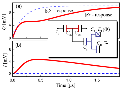
Figure 1: Time evolution of the quadratures, $Q$ (a) and $I$ (b), for the parameters of Ref. [Bianchetti et al., 2009] for the two situations, when the qubit was initialized in either the ground or excited state, denoted as “$\left|g\right\rangle$-response” and “$\left|e\right\rangle$-response”, respectively. The inset presents the scheme of the transmon-type qubit coupled to the transmission-line resonator.

The driven transmon-resonator system Koch et al. (2007); Bianchetti et al. (2009); Bishop et al. (2009) is described by the Jaynes-Cummings Hamiltonian Schleich (2001)

$$H = \hbar\omega_{\mathrm{r}}a^{{\dagger}}a+\hbar\frac{\omega_{\mathrm{q}}}{2}\sigma_{z}+\hbar\mathrm{g}\left(\sigma a^{{\dagger}}+\sigma^{{\dagger}}a\right)+$$

$$+\hbar\xi\left(a^{{\dagger}}e^{-i\omega t}+ae^{i\omega t}\right).$$

Here the transmon is considered in the two-level approximation, described by the energy distance $\hbar\omega_{\mathrm{q}}$ between the levels and the Pauli operators $\sigma_{i}$ and $\sigma_{\pm}=\left(\sigma_{x}\pm i\sigma_{y}\right)/2$, where we rather use the ladder-operator notations $\sigma\equiv\sigma_{-}$ and $\sigma^{{\dagger}}\equiv\sigma_{+}$; the resonator is described by the resonant frequency $\omega_{\mathrm{r}}$ and the annihilation operator $a$; the transmon-resonator coupling constant $\mathrm{g}$ relates to the bare coupling $\mathrm{g}_{0}$ as $\mathrm{g}=\mathrm{g}_{0}\sqrt{E_{\mathrm{c}}/\left|\Delta-E_{\mathrm{c}}\right|}$ with $\Delta=\hbar\left(\omega_{\mathrm{q}}-\omega_{\mathrm{r}}\right)$ (this renormalization is due to the virtual transitions through the upper transmon’s states); the probing signal is described by the amplitude $\xi$ and frequency $\omega$.

The system’s dynamics obeys the master equation, which is described in Appendix A. There, it is demonstrated that the Lindblad equation for the density matrix can be rewritten as an infinite set of equations for the expectation values. In Refs. [Bianchetti et al., 2009; Shevchenko et al., 2014] the set of equations was reduced to six complex equations for the single expectation values and the two-operator correlators. Meanwhile, many quantum-optical phenomena can be described within the semiclassical theory, assuming all the correlation functions to factorize (e.g. Refs. [Mu and Savage, 1992; Hauss et al., 2008; André et al., 2009; Macha et al., 2014]). This approach results in that the system’s dynamics is described by the set of three equations only, Eqs. (30), which are more suitable for analytic consideration, as we will see below. This was also analyzed in Ref. [Shevchenko et al., 2014]; in particular, the robustness of the semiclassical approximation was demonstrated even in the limit of small photon number, at small probing amplitude $\xi$.

The observable value can be either transmission signal amplitude or the quadrature amplitudes. The quadratures of the transmitted field $I$ and $Q$ are related to the cavity field $\left\langle a\right\rangle$ as following Bianchetti et al. (2009); Bishop et al. (2009)

$$I=2V_{0}\,\,\text{Re}\left\langle a\right\rangle\text{, \ }Q=2V_{0}\,\,\text{Im}\left\langle a\right\rangle,$$ (2)

where $V_{0}$ is a voltage related to the gain of the experimental amplification chain Bishop et al. (2009) and it is defined as Bianchetti et al. (2009) $V_{0}^{2}=Z\hbar\omega_{\mathrm{r}}\varkappa/4$ with $Z$ standing for the transmission-line impedance. The transmission amplitude $A$ is given Bishop et al. (2009); Macha et al. (2014) by the absolute value of $\left\langle a\right\rangle$

$$A=\sqrt{I^{2}+Q^{2}}=2V_{0}\left|\left\langle a\right\rangle\right|.$$ (3)

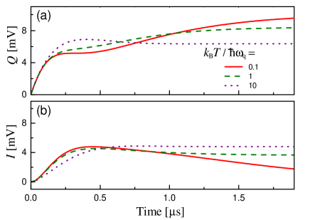
Figure 2: Time evolution of the quadratures, $Q$ (a) and $I$ (b), for non-zero temperature $T$. The situation when the qubit was initialized in the excited state is considered. The parameters are the same as in Fig. 1, besides the temperature, so that the solid red curves for the low temperature repeat the ones from the previous figure.

As an illustration of the semiclassical theory, presented in more detail in Appendix A, consider the experimental realization in Ref. [Bianchetti et al., 2009]. There, the qubit was initialized in either ground or excited state and then, by means of either continuous or pulsed measurements, the quadratures of the transmitted field were probed. Correspondingly, we make use of Eqs. (2) and (30), which include the resonator relaxation rate $\varkappa$ and the qubit decoherence rate $\Gamma_{2}=\Gamma_{\phi}+\Gamma_{1}/2$ with $\Gamma_{\phi}$ and $\Gamma_{1}$ being the intrinsic qubit pure dephasing and relaxation rates. We take the following parameters Bianchetti et al. (2009): $\omega_{\mathrm{r}}/2\pi=6.4425$ GHz, $\omega_{\mathrm{q}}/2\pi=4.01$ GHz, $\mathrm{g}_{0}/2\pi=134$ MHz,$\ \varkappa/2\pi=1.7$ MHz, $\Gamma_{1}/2\pi=0.2$ MHz, $\Gamma_{2}=\Gamma_{1}/2$, $E_{\mathrm{c}}/h=232$ MHz, and $V_{0}=5$ mV, where the latter was chosen as a fitting parameter. The results for low temperature (i.e. for $k_{\mathrm{B}}T\ll\hbar\omega_{{}_{\mathrm{q}}}$) are presented in Fig. 1. Note the agreement with the experimental observations in Ref. [Bianchetti et al., 2009]; see also detailed calculations in Appendix B below. There, in Ref. [Bianchetti et al., 2009] it is discussed in detail that the relaxation of the quadratures is determined for the ground-state formulation by the resonator rate $\varkappa$ only, while for the excited-state formulation this is determined by the collaborative evolution of the qubit-resonator system. For example, one can observe that the relaxation of the quadratures in Fig. 1 for the “$\left|e\right\rangle$-response” happens in two stages, during the times $T_{\varkappa}=2\pi/\varkappa\simeq 0.6\mu$s and $T_{1}=2\pi/\Gamma_{1}\gg T_{\varkappa}$.

III Thermometry with continuous measurements

In previous Section we calculated the low-temperature behaviour of the observable quadratures for the qubit-resonator system and illustrated this in Fig. 1. Having obtained the agreement with the experimental observations of Ref. Bianchetti et al. (2009), we can proceed with posing other problems for the system. Consider now the sensitivity of the system to the changes of temperature. How the behaviour of the observables changes? Is this useful for a single-qubit thermometry? To respond to such questions, we describe below both dynamical and stationary behaviour for non-zero temperature.

In Fig. 2 we plot the time evolution of the quadratures for the same parameters as in Fig. 1 besides the temperature, which now is considered non-zero. Figure 2 demonstrates that both evolution and stationary values (at long times, independent of initial conditions) are strongly temperature dependent.

To further explore the temperature dependence, we now consider the steady-state measurements. In equilibrium, the observables are described by the steady-state values of $\left\langle a\right\rangle$, $\left\langle\sigma\right\rangle$, and $\left\langle\sigma_{z}\right\rangle$. The steady-state solution for the weak driving amplitude in the semiclassical approximation is the following (for details see Appendix A):

$$\left\langle a\right\rangle=-\xi\frac{\delta\omega_{\mathrm{q}}^{\prime}}{\left\langle\sigma_{z}\right\rangle\mathrm{g}^{2}+\delta\omega_{\mathrm{q}}^{\prime}\delta\omega_{\mathrm{r}}^{\prime}},$$ (4)

where

$$\delta\omega_{\mathrm{r}}^{\prime} = \omega_{\mathrm{r}}-\omega-i\frac{\varkappa}{2},\text{ }\delta\omega_{\mathrm{q}}^{\prime}=\omega_{\mathrm{q}}-\omega-i\frac{\Gamma_{2}}{z_{0}},$$ (5)

$$z_{0} = \tanh\left(\frac{\hbar\omega_{{}_{\mathrm{q}}}}{2k_{\mathrm{B}}T}\right).$$

In equilibrium, the qubit energy-level populations are defined by the temperature $T$: $\left\langle\sigma_{z}\right\rangle=-z_{0}$ Jin et al. (2015). Importantly, formula (4) bears the information about the qubit temperature and via formula (3) brings this dependence to the observables.

Formula (4) is quite general. To start with, for an isolated resonator (without qubit) at $\mathrm{g}=0$ this gives

$$\left|\left\langle a\right\rangle\right|^{2}=\xi^{2}\frac{1}{\delta\omega_{\mathrm{r}}^{2}+\varkappa^{2}/4},$$ (6)

which defines the resonator width.

Consider now the dispersive limit, where $\Delta/\hbar\equiv\omega_{\mathrm{q}}(\Phi)-\omega_{\mathrm{r}}\gg\mathrm{g}/h,\,\,\delta\omega_{\mathrm{r}}$. Then we have for the transmission amplitude

$$\left|\left\langle a\right\rangle\right|^{2}\approx\xi^{2}\frac{\Delta^{2}}{\left(\left\langle\sigma_{z}\right\rangle\mathrm{g}^{2}+\Delta\delta\omega_{\mathrm{r}}\right)^{2}+\Delta^{2}\varkappa^{2}/4}.$$ (7)

This, in particular, gives the maxima for the transmission at

$$\delta\omega_{\mathrm{r}}=-\left\langle\sigma_{z}\right\rangle\frac{\mathrm{g}^{2}}{\Delta}\equiv-\left\langle\sigma_{z}\right\rangle\chi.$$ (8)

Then, for the ground/excited states with $\left\langle\sigma_{z}\right\rangle=\mp 1$, one obtains the two dispersive shifts for the maximal transmission, $\delta\omega_{\mathrm{r}}=\pm\chi=\pm\mathrm{g}_{0}^{2}E_{\mathrm{c}}/\Delta(\Delta-E_{\mathrm{c}})$, respectively. In thermal equilibrium, equation (8) for the resonance frequency shift gives $\delta\omega_{\mathrm{r}}(T)=\frac{\mathrm{g}^{2}}{\Delta}\tanh\left(\frac{\hbar\omega_{{}_{\mathrm{q}}}}{2k_{\mathrm{B}}T}\right)$.

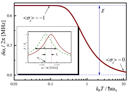
Figure 3: Transmission amplitude and the frequency shift. First, the inset shows the transmission amplitude $A$ versus the frequency $\omega$ when the qubit is either in the ground state (solid line) or in the excited state (dashed line). Then, the main panel demonstrates the frequency shift $\delta\omega_{\mathrm{r}}=\omega_{\mathrm{r}}-\omega$, corresponding to the frequency $\omega$ at which the transmission is maximal, plotted as a function of temperature $T$. Here the transmission amplitude is normalized with $A_{0}=4V_{0}\mathrm{g}\xi/\varkappa$.

Making use of Eqs. (3) and (7) in thermal equilibrium, when $\left\langle\sigma_{z}\right\rangle=-z_{0}$, in the inset in Fig. 3 we plot the frequency dependence of the transmission amplitude for the parameters of Ref. [Bianchetti et al., 2009]. We plot two cuves, where the solid one corresponds to a low-temperature limit ($z_{0}=1$) with the system in the ground state, while the dashed line is plotted in a high-temperature limit ($z_{0}=0$), when the system is in the superposition of the ground and excited state. The maximal frequency shift is denoted with $\chi$. Note that the low-temperature limit (solid line in the inset), with $\left\langle\sigma_{z}\right\rangle\sim-1$, corresponds to the ground state, while the high-temperature limit (dashed line), with $\left\langle\sigma_{z}\right\rangle\sim 0$, is equivalent to the absence of the qubit, at $\mathrm{g}=0$.

For varying temperature, the frequency shift is plotted in the main panel of Fig. 3, for the parameters of Ref. [Bianchetti et al., 2009]. We note that similar dependence can be found in Fig. 4.2 of Ref. [Bianchetti, 2010]; the difference is in that in the case of Refs. [Bianchetti et al., 2009; Bianchetti, 2010] similar change of $\left\langle\sigma_{z}\right\rangle$ from $-1$ to $0$ was due to varying the driving power. When driven with low power, qubit stayed in the ground state with $\left\langle\sigma_{z}\right\rangle=-1$, while with increasing the power its stationary state tended to equally populated states with $\left\langle\sigma_{z}\right\rangle=0$. Also, to this case of varying the qubit driving, we further devote Appendix C.

The temperature dependence in Fig. 3 becomes apparent at $T\geq T^{\ast}$, where $T^{\ast}=0.1\hbar\omega_{{}_{\mathrm{q}}}/k_{\mathrm{B}}$ is the characteristic temperature, which, say, for $\omega_{{}_{\mathrm{q}}}/2\pi=4$ GHz is quite low, $T^{\ast}=20$ mK. This means that such measurements may be useful for realizing the one-qubit thermometry for $T\geq T^{\ast}$.

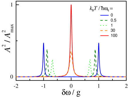
Figure 4: Transmission $A^{2}$, normalized with its maximal value $A_{\max}$, versus the frequency shift $\delta\omega$ for different values of temperature $T$.

It is important to note that Eq. (4) was obtained without making use of the dispersive limit, and thus this is applicable to the opposite limit. Consider in this way $\omega_{{}_{\mathrm{q}}}(\Phi)=\omega_{{}_{\mathrm{r}}}$, which is the resonant limit, $\Delta=0$. With equal detunings for both qubit and resonator, $\omega_{\mathrm{q}}-\omega=\omega_{\mathrm{r}}-\omega\equiv\delta\omega$, we can use the formula for the photon operator, Eq. (4), which gives

$$\left|\left\langle a\right\rangle\right|^{2}\approx\xi^{2}\frac{\delta\omega^{2}+\Gamma_{2}^{2}/z_{0}^{2}}{\left(\left\langle\sigma_{z}\right\rangle\mathrm{g}^{2}+\delta\omega^{2}\right)^{2}+\delta\omega^{2}\left(\Gamma_{2}/z_{0}+\varkappa/2\right)^{2}}.$$ (9)

With this we plot the transmission amplitude as a function of the frequency detuning in Fig. 4 for different temperatures. Formula (9) describes maxima, which, assuming large cooperativity $\mathrm{g}^{2}/\Gamma_{2}\varkappa\gg 1$, are situated at $\delta\omega=0$ (the high-temperature peak) and at

$$\delta\omega\approx\pm\mathrm{g}\tanh^{1/2}\left(\frac{\hbar\omega_{{}_{\mathrm{q}}}}{2k_{\mathrm{B}}T}\right).$$ (10)

The latter formula, in particular, in the low-temperature limit describes the peaks at $\delta\omega=\pm\mathrm{g}$, which is known as the vacuum Rabi splitting. Note that recently such vacuum Rabi splitting was also demonstrated in silicon qubits in Ref. [Mi et al., 2016]. With increasing the qubit temperature, equation (10) means the temperature-dependent resonance-frequency shift. We note, that this shift is again described by the factor $\left\langle\sigma_{z}\right\rangle=-z_{0}$. If we assume here the qubit in the ground state, $\left\langle\sigma_{z}\right\rangle=-1$, then the increase of the temperature would result in suppressing the peaks at $\delta\omega=\pm\mathrm{g}$, without their shift, in agreement with Ref. [Fink et al., 2010].

IV Thermometry with pulsed measurements

Above we have considered the case when the measurement is done in a weak continuous manner. Then, the resonator probes the averaged qubit state, defined by $\left\langle\sigma_{z}\right\rangle$, and changing the qubit state resulted in shifting the position of the resonant transmission. Alternatively, the measurements can be done with the single-shot readout Reed et al. (2010); Jin et al. (2015); Jerger et al. (2016a, b); Reagor et al. (2016). In this case, in each measurement, the resonator would see the qubit in either the ground or excited state, with $\left\langle\sigma_{z}\right\rangle$ equal to $-1$ or $1$, respectively Vijay et al. (2011). Probability of finding the qubit in the excited state is $P_{+}$ and in the ground state: $P_{-}=1-P_{+}$. Then, the weighted (averaged over many measurements) transmission amplitude can be calculated as following

$$A=P_{-}A_{-}+P_{+}A_{+},$$ (11)

where $A_{\pm}$ describe the transmission amplitudes calculated for $\left\langle\sigma_{z}\right\rangle=\pm 1$, respectively, as given by Eq. (7).

We may now consider two cases, of a qubit driven resonantly and when the excitation happens due to the temperature. In the former case, when a qubit is driven with frequency $\omega_{\mathrm{d}}=\omega_{\mathrm{q}}$ and amplitude $\hbar\Omega$, the excited qubit state is populated with the probability

$$P_{+}(\Omega) = \frac{1}{2}\left[1+\overline{\Omega}^{-2}\right]^{-1},$$ (12)

$$\overline{\Omega} = \frac{1}{2}\hbar\Omega\sqrt{T_{1}T_{2}}.$$

This is obtained from the full formula for a qubit excited near the resonant frequency Shevchenko et al. (2014):

$$P_{+}=\frac{1}{2}\frac{\omega_{\mathrm{q}}^{2}J_{1}^{2}\left(\frac{\Omega}{\omega_{\mathrm{d}}}\right)}{\omega_{\mathrm{q}}^{2}J_{1}^{2}\left(\frac{\Omega}{\omega_{\mathrm{d}}}\right)+\frac{T_{2}}{T_{1}}\left(\omega_{\mathrm{q}}-\omega_{\mathrm{d}}\right)^{2}+\frac{1}{T_{1}T_{2}}},$$ (13)

where we then take $\omega_{\mathrm{d}}=\omega_{\mathrm{q}}$ and $J_{1}(x)\approx x/2$.

In thermal equilibrium the upper-level occupation probability is defined by the Maxwell-Boltzmann distribution, $\left\langle\sigma_{z}\right\rangle=-z_{0}$ Jin et al. (2015), so that $P_{+}=\frac{1}{2}\left[1+\left\langle\sigma_{z}\right\rangle\right]$ or

$$P_{+}(T)=\frac{1}{2}\left[1-\tanh\left(\frac{\hbar\omega_{{}_{\mathrm{q}}}}{2k_{\mathrm{B}}T}\right)\right].$$ (14)

With these equations (12) and (14) we calculate the transmission amplitude, when the qubit was either resonantly driven (Fig. 5) or in a thermal equilibrium (Fig. 6), respectively. For the former case we plot the frequency dependence of the transmission amplitude in Fig. 5. Similar dependence would be for varying temperature; in Fig. 6 we rather present the transmission amplitude versus temperature for a fixed frequency $\omega=\omega_{\mathrm{r}}+\chi=\omega_{\mathrm{r}}-\left|\chi\right|$, where the excited-state peak appears. For calculations we took here the parameters close to the ones of Ref. [Jin et al., 2015]: $\omega_{\mathrm{r}}/2\pi=10.976$ GHz, $\omega_{\mathrm{q}}/2\pi=4.97$ GHz, $\chi/2\pi=-4$ MHz, and we have chosen$\ \varkappa/2\pi=1$ MHz. Again, as above, we observe strong dependence on temperature. Advantages of probing qubit state in a similar manner were discussed in Ref. [Reed et al., 2010]. There, it was proposed to probe a driven qubit state, while our proposal here relates to the thermal-equilibrium measurement and consists in providing sensitive tool for thermometry. Indeed, similar temperature dependence was recently observed by Jin et al. in Ref. [Jin et al., 2015]. In that work the authors studied the excited-state occupation probability in a transmon with variable temperature. For comparison with that publication, in the inset of Fig. 6 we also present the low-temperature region, with linear scale.

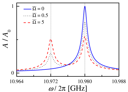
Figure 5: Transmission amplitude for monitoring the state of a driven qubit. The frequency $\omega$ is in the range from $\omega_{\mathrm{r}}-3\left|\chi\right|$ to $\omega_{\mathrm{r}}+3\left|\chi\right|$. The peak corresponding to the ground state is at $\omega_{\mathrm{r}}+\left|\chi\right|=10.98$ GHz$\cdot 2\pi$. The peak appearing for non-zero occupation of the excited state is at $\omega=\omega_{\mathrm{r}}-\left|\chi\right|=10.972$ GHz$\cdot 2\pi$. The height of the latter is defined by the normalized driving amplitude $\overline{\Omega}$.

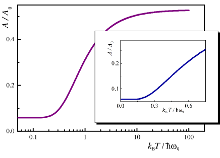
Figure 6: Temperature dependence of the transmission amplitude $A$ at the frequency corresponding to the excited-state peak, which is $\omega=\omega_{\mathrm{r}}-\left|\chi\right|$ in the previous figure. Inset demonstrates the low-temperature region.

V Memcapacitance

Now, having reached the agreement of the theory with the experiments, we wish to explore other applications. In this section we mean possibilities for memory devices, such as memcapacitors.

In general, a memory device with the input $u(t)$ and the output $y(t)$, by definition, is described by the following relations Di Ventra et al. (2009)

$$y(t) = g(\mathbf{x},u,t)u(t),$$ (15)

$$\mathbf{\dot{x}} = \mathbf{f}(\mathbf{x},u,t).$$ (16)

Here $g$ is the response function, while the vector function $\mathbf{f}$ defines the evolution of the internal variables, denoted as a vector $\mathbf{x}$. Depending on the choice of the circuit variables $u$ and $y$, the relations (15-16) describe memristive, meminductive, or memcapacitive systems. Relevant for our consideration is the particular case of the voltage-controlled memcapacitive systems, defined by the relations

$$q(t) = C_{\mathrm{M}}(\mathbf{x},V,t)V(t),$$ (17)

$$\mathbf{\dot{x}} = \mathbf{f}(\mathbf{x},V,t).$$ (18)

Here the response function $C_{\mathrm{M}}$ is called the memcapacitance.

Relations (15-16) and their particular case, Eqs. (17-18), were related to diverse systems, as described e.g. in the review article [Pershin and Di Ventra, 2011]. It was shown that the reinterpretation of known phenomena in terms of these relations makes them useful for memory devices. However, until recently their quantum analogues remained unexplored. Then, some similarities and distinctions from classical systems were analyzed in Refs. [Pfeiffer et al., 2016; Shevchenko et al., 2016; Salmilehto et al., 2017; Li et al., 2017; Sanz et al., 2017]. In particular, it was argued that in the case of quantum systems, the circuit input and output variables $u$ and $y$ should be interpreted as quantum-mechanically averaged values or in the ensemble interpretation Shevchenko et al. (2016); Salmilehto et al. (2017). Detailed analysis of diverse systems Pfeiffer et al. (2016); Shevchenko et al. (2016); Salmilehto et al. (2017); Li et al. (2017); Sanz et al. (2017) demonstrated that, being described by relations (15-16), quantum systems could be considered as quantum memristors, meminductors, and memcapacitors. These indeed displayed the pinched-hysteresis loops for periodic input, while the frequency dependence may significantly differ from the related classical devices. The former distinction is due to the probabilistic character of measurements in quantum mechanics. Note that the “pinched-hysteretic loop” dependence is arguably the most important property of memristors, meminductors, and memcapacitors.Di Ventra et al. (2009); Pershin and Di Ventra (2011)

It is thus our goal in this section to demonstrate how the evolution equations for a qubit-resonator system can be written in the form of the memcapacitor relations, Eqs. (17-18). This would allow us to identify the related input and output variables, the internal-state variables, the response and evolution functions. As a further evidence, we will demonstrate one particular example, when for a resonant driving the pinched-hysteresis loop appears.

The transmon treated as a memcapacitor is depicted in Fig. 7(a). As an input of such a memcapacitor we assume the resonator antinode voltage $V$ (how a transmon is coupled to a transmission-line resonator was shown in Fig. 1), while the output is the charge $q$ on the external plate of the gate capacitor $C_{\mathrm{g}}$. One should differentiate between the externally applied voltage, $V_{\mathrm{g}}=V_{A}\sin\omega t$, and the quantized antinode voltage,

$$V=\left\langle\widehat{V}\right\rangle=V_{\mathrm{rms}}\left\langle ae^{-i\omega t}+a^{{\dagger}}e^{i\omega t}\right\rangle=2V_{\mathrm{rms}}\text{Re}\left\langle ae^{-i\omega t}\right\rangle,$$ (19)

where $V_{\mathrm{rms}}=\sqrt{\hbar\omega_{\mathrm{r}}/2C_{\mathrm{r}}}$ is the root-mean-square voltage of the resonator, defined by its resonant frequency $\omega_{\mathrm{r}}$  and capacitance $C_{\mathrm{r}}$.Koch et al. (2007) This makes the difference from a charge qubit coupled directly to a gate, such as in Ref. [Shevchenko et al., 2016]. Accordingly to Eq. (19), the voltage is related to the measurable values, the resonator output field quadratures, Eq. (2). The charge $q$ is related to the voltage $V$ and the island charge $2e\left\langle n\right\rangle$ ($\left\langle n\right\rangle$ is the average Cooper-pair number) as following Shevchenko et al. (2016):

$$q=C_{\mathrm{geom}}V+\frac{C_{\mathrm{g}}}{C_{\Sigma}}2e\left\langle n\right\rangle\equiv C_{\mathrm{M}}V,$$ (20)

where we formally introduced the memcapacitance $C_{\mathrm{M}}$ as a proportionality coefficient between the input $V$ and the output $q$. Given the leading role of the shunt capacitance, here we have $C_{\Sigma}=C_{J}+C_{\mathrm{g}}+C_{B}\sim C_{B}$ and $C_{\mathrm{geom}}=C_{\mathrm{g}}(C_{J}+C_{B})/C_{\Sigma}\approx C_{\mathrm{g}}$. The number operator $n$ is defined by the qubit Pauli matrix $\sigma_{y}$: $n=\frac{1}{4}\sqrt{\hbar\omega_{{}_{\mathrm{q}}}/E_{\mathrm{c}}}\sigma_{y}$. This allows us rewriting Eq. (20),

$$\widetilde{q}=\text{Re\negthinspace}\left\langle a\right\rangle\cos\omega t-\text{Im\negthinspace}\left\langle a\right\rangle\sin\omega t+\lambda\left\langle\sigma_{y}\right\rangle,$$ (21)

where $\widetilde{q}=q/2C_{\mathrm{g}}V_{\mathrm{rms}}$ and $\lambda=(e/4C_{\Sigma}V_{\mathrm{rms}})\sqrt{\hbar\omega_{{}_{\mathrm{q}}}/E_{\mathrm{c}}}$. We note that in related experiments, not only the quadratures $I$ and $Q$ (which define Re$\left\langle a\right\rangle$ and Im$\left\langle a\right\rangle$), but also the qubit state, defined by the values $\left\langle\sigma_{z}\right\rangle$ and $\left\langle\sigma_{y}\right\rangle$, can be reliably probed, see Refs. [Filipp et al., 2009; Bianchetti et al., 2009; McClure et al., 2016; Gong et al., 2016; Jerger et al., 2017]. Importantly, the memcapacitor’s dynamics, i.e. $q(t)$, is defined by rich dynamics of both the resonator and the qubit, via $\left\langle a\right\rangle$ and $\left\langle\sigma_{y}\right\rangle$, respectively.

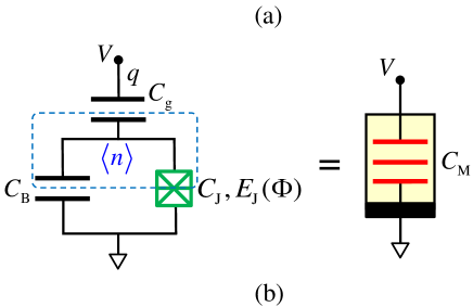
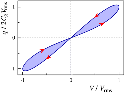
Figure 7: A transmon qubit can be accounted as a memcapacitor. (a) Scheme of a transmon-type qubit is shown to be equivalent to a memcapacitor $C_{\mathrm{M}}$, of which the symbol is shown to the right. (b) Pinched-hysteretic curve in the voltage-charge plane as a fingerprint of a memcapacitive behaviour.

Importantly, here we have written the transmon-resonator equations in the form of the memcapacitor first relation, Eq. (17). We can see that the role of the internal variables is played by the qubit charge $\left\langle n\right\rangle$. In its turn, the qubit state is defined by the Lindblad equation, which now takes place of the second memcapacitor relation, Eq. (18). Such formulation demonstrates that our qubit-resonator system can be interpreted as a quantum memcapacitor, which is schematically displayed in Fig. 7(a).

The above formulas allow us to plot the charge–versus–voltage diagram. For this we assume now that the qubit is driven by the field with amplitude $\Omega$ and frequency $\omega_{\mathrm{d}}$, which is resonant, $\omega_{\mathrm{d}}=\omega_{\mathrm{q}}(\Phi)$. This induces Rabi oscillations in the qubit with the frequency $\Omega$. By numerically solving Eqs. (5a-5d) in Ref. [Bianchetti et al., 2009], we plot the $q$ versus $V$ diagram in Fig. 7(b). To obtain the pinched-hysteresis-type loop, we take the driving amplitude, $\Omega=2\omega_{\mathrm{r}}$, which corresponds to the strong-driving regime. Other system parameters are the same as used above (the ones of Ref. [Bianchetti et al., 2009]) and $\lambda=0.2$. In addition we have taken Re$\left\langle a\right\rangle=0$ and Im$\left\langle a\right\rangle=1$. Here we note that $\left\langle a\right\rangle$ is a slow function of time, as demonstrated in Fig. 1. (The characteristic time for this is $2\pi/\varkappa$, which is $\gg$ $2\pi/\Omega$.) Moreover, the diagram is not only defined by $\lambda$ (which is a constant), but also by $\left\langle a\right\rangle$ (which can be adjusted, for example, by choosing a moment of time in Fig. 1); so, for a different value of $\lambda$ another value of $\left\langle a\right\rangle$ can be taken. We note that the shaded area in Fig. 7(b) equals to the energy consumed by the memcapacitor, $\int VIdt$.Pershin and Di Ventra (2011)

Note that we made use of the two-level approximation for the transmon, and, on the other hand considered the strong-driving regime, where $\Omega=2\omega_{\mathrm{r}}$. This was needed for demonstrating the pinched-hysteresis loop by illustrative means. While the strong-driving regime was demonstrated in many types of qubits, in the transmon ones this is complicated due to the weak anharmonicity, which may result in transitions to the upper levels (cf. Refs. [Gong et al., 2016; Lu et al., 2017; Dai et al., 2017] though). In this way, one would have to confirm the calculations with the more elaborated ones, by taking into account the higher levels (as e.g. in Refs. [Peterer et al., 2015; Pietikäinen et al., 2017, 2018], see also our discussion below, in Appendix C) and clarify the relation, needed for the hysteretic-type loops. Alternatively, one may think of the readily observed Rabi oscillations in the megahertz domain and combine these with the oscillations related to another resonator. At such low frequency the resonator may be considered as classical, similarly to calculations in Ref. [Shevchenko et al., 2016].

VI Conclusion

We have considered the qubit-resonator system, accentuating on the situation with a transmon-type qubit in a transmission-line resonator. The most straightforward approach is the semiclassical theory, when all the correlators are assumed to factorize, which has the advantage of getting transparent analytical equations and formulas. We demonstrated that with this we can describe relevant experiments Bianchetti et al. (2009); Jin et al. (2015); Pietikäinen et al. (2017). On the other hand, the validity of the semiclassical theory was checked with the approach taking into account the two-operator qubit-photon correlators, so-called semi-quantum approach. Furthermore, we included temperature into consideration and studied its impact on the measurable quadratures of the transmitted field. Due to the qubit-resonator entanglement, the resonator transmission bears information about the temperature experienced by the qubit. Consideration of this application, the thermometry, was followed by another one, the memory device, known as a memcapacitor. As a proof-of-concept, we demonstrated the pinched hysteretic loop in the charge-voltage plane, the fingerprint of memcapacitance. In the case with qubits, this loop is related to the Rabi-type oscillations. We believe that such quantum memcapacitors, along with quantum meminductors and memristors, will add new functionality to the toolbox of their classical counterparts.

Appendix A Lindblad and Maxwell-Bloch equations

Consider how starting from the Hamiltonian (II), we get the motion equations in the semiclassical approximation and obtain the steady-state value for the photon operator in Eq. (4).

First, the Hamiltonian (II) is transformed with the operator $U=\exp\left[i\omega t\left(a^{{\dagger}}a+\sigma_{z}/2\right)\right]$ to the following $H^{\prime}=UHU^{{\dagger}}+i\hbar\dot{U}U^{{\dagger}}$ (see e.g. Ref. [Shevchenko et al., 2014]):

$$H^{\prime}=\hbar\delta\omega_{\mathrm{r}}a^{{\dagger}}a+\hbar\frac{\delta\omega_{\mathrm{q}}}{2}\sigma_{z}+\hbar\mathrm{g}\left(\sigma a^{{\dagger}}+\sigma^{{\dagger}}a\right)+\hbar\xi\left(a^{{\dagger}}+a\right),$$ (22)

where

$$\delta\omega_{\mathrm{r}}=\omega_{\mathrm{r}}-\omega,~{}~{}\delta\omega_{\mathrm{q}}=\omega_{\mathrm{q}}-\omega.$$ (23)

Then, the system’s dynamics is described by the Lindblad master equation

$$\dot{\rho}=-\frac{i}{\hbar}\left[H^{\prime},\rho\right]+\varkappa\mathcal{D}\left[a\right]\rho+\Gamma_{1}\mathcal{D}\left[\sigma\right]\rho+\frac{\Gamma_{\phi}}{2}\mathcal{D}\left[\sigma_{z}\right]\rho,$$ (24)

where the damping terms model the loss of cavity photons at rate $\varkappa$, as well as the intrinsic qubit relaxation and pure dephasing at rates $\Gamma_{1}$ and $\Gamma_{\phi}$. The respective Lindblad damping superoperators at non-zero temperature $T$ are given by Scully and Zubairy (1997)

$$\!\!\!\!\!\!\!\!\mathcal{D}\left[a\right]\rho\!\! = \!\!\left(N_{\mathrm{th}}+1\right)\left(a\rho a^{{\dagger}}-\frac{1}{2}\left\{a^{{\dagger}}a,\rho\right\}\right)+$$

$$+N_{\mathrm{th}}\left(a^{{\dagger}}\rho a-\frac{1}{2}\left\{aa^{{\dagger}},\rho\right\}\right),$$

$$\!\!\!\!\!\!\!\!\mathcal{D}\left[\sigma\right]\rho\!\! = \!\!\left(n_{\mathrm{th}}+1\right)\left(\sigma\rho\sigma^{{\dagger}}-\frac{1}{2}\left\{\sigma^{{\dagger}}\sigma,\rho\right\}\right)+$$

$$+n_{\mathrm{th}}\left(\sigma^{{\dagger}}\rho\sigma-\frac{1}{2}\left\{\sigma\sigma^{{\dagger}},\rho\right\}\right),$$

$$\!\!\!\!\!\!\!\!\mathcal{D}\left[\sigma_{z}\right]\rho\!\! = \!\!\left(2n_{\mathrm{th}}+1\right)\left(\sigma_{z}\rho\sigma_{z}-\rho\right),\!\!\!$$ (25c)

$$N_{\mathrm{th}}\!\!=\!\!\left(\exp\!\!\left(\frac{\hbar\omega_{\mathrm{r}}}{k_{\mathrm{B}}T}\right)-1\right)^{-1}\!\!,~{}n_{\mathrm{th}}\!\!=\!\!\left(\exp\!\!\left(\frac{\hbar\omega_{{}_{\mathrm{q}}}}{k_{\mathrm{B}}T}\right)-1\right)^{-1}\!.$$ (26)

In particular, at $T=0$: $N_{\mathrm{th}}=n_{\mathrm{th}}=0$.

From the Lindblad equation (24), for the expectation values of the operators $a$, $\sigma$, and $\sigma_{z}$ we obtain the following system of equations (as in Refs. [Shevchenko et al., 2014; Hauss et al., 2008]):

$$\!\!\!\!\!\!\!\!\!\!\!\!\frac{d\left\langle a\right\rangle}{dt}\!\! = \!\!-i\delta\omega_{\mathrm{r}}^{\prime}\left\langle a\right\rangle-i\mathrm{g}\left\langle\sigma\right\rangle-i\xi,$$ (27a)

$$\!\!\!\!\!\!\!\!\!\!\!\!\frac{d\left\langle\sigma\right\rangle}{dt}\!\! = \!\!-i\delta\omega_{\mathrm{q}}^{\prime}\left\langle\sigma\right\rangle+i\mathrm{g}\left\langle a\sigma_{z}\right\rangle,$$ (27b)

$$\!\!\!\!\!\!\!\!\!\!\!\!\frac{d\left\langle\sigma_{z}\right\rangle}{dt}\!\! = \!\!-i2\mathrm{g}\left(\left\langle a\sigma^{{\dagger}}\right\rangle\!-\!\left\langle a^{{\dagger}}\sigma\right\rangle\right)-\Gamma_{1}\left(\!1\!+\!\frac{\left\langle\sigma_{z}\right\rangle}{z_{0}}\!\right)\!,$$ (27c)

where

$$\delta\omega_{\mathrm{r}}^{\prime} = \delta\omega_{\mathrm{r}}-i\frac{\varkappa}{2},\text{ }\delta\omega_{\mathrm{q}}^{\prime}=\delta\omega_{\mathrm{q}}-i\frac{\Gamma_{2}}{z_{0}},\text{ }$$ (28)

$$z_{0} = \tanh\left(\frac{\hbar\omega_{{}_{\mathrm{q}}}}{2k_{\mathrm{B}}T}\right),~{}\Gamma_{2}=\Gamma_{\phi}+\frac{\Gamma_{1}}{2}.$$

The meaning of the value $z_{0}$ is in describing the qubit temperature-dependent equilibrium population, which is seen from Eq. (27c), if neglecting the coupling $\mathrm{g}$.

The system of equations (27) becomes closed under the assumption that all the correlation functions factorize (e.g. Ref. [Hauss et al., 2008]). Then for the classical variables

$$\alpha=\left\langle a\right\rangle,\quad s=\left\langle\sigma\right\rangle,\quad s_{z}=\left\langle\sigma_{z}\right\rangle$$ (29)

we obtain the equations, which are also called the Maxwell-Bloch equations,

$$\dot{\alpha} = -i\delta\omega_{\mathrm{r}}^{\prime}\alpha-i\mathrm{g}s-i\xi,$$ (30a)

$$\dot{s} = -i\delta\omega_{\mathrm{q}}^{\prime}s+i\mathrm{g}\alpha s_{z},$$ (30b)

$$\dot{s}_{z} = -i2\mathrm{g}\left(\alpha s^{\ast}-\alpha^{\ast}s\right)-\Gamma_{1}\left(1+\frac{s_{z}}{z_{0}}\right).$$ (30c)

This system of equations is convenient for describing the dynamics, as we do in the main text. Also, these equations are simplified for the steady state, where the time derivatives in the l.h.s. are zeros. Then for $$\alpha s_{z}$$ and , we obtain

$$\alpha = -\xi\frac{\delta\omega_{\mathrm{q}}^{\prime}}{s_{z}\mathrm{g}^{2}+\delta\omega_{\mathrm{q}}^{\prime}\delta\omega_{\mathrm{r}}^{\prime}},$$ (31)

$$s_{z} = -z_{0}+\frac{2z_{0}}{\Gamma_{1}}\left(\varkappa\left|\alpha\right|^{2}+2\xi\text{Im}\alpha\right).$$ (32)

These are further simplified in the low probing-amplitude limit. In this case we note that $\alpha\sim\xi$ and obtain

$$s_{z} = -z_{0},$$ (33)

$$\alpha = \xi\frac{\delta\omega_{\mathrm{q}}^{\prime}}{z_{0}\mathrm{g}^{2}-\delta\omega_{\mathrm{q}}^{\prime}\delta\omega_{\mathrm{r}}^{\prime}}.$$ (34)

These formulas are analyzed in the main text.

Appendix B Semi-quantum model with temperature

Here, following Refs. [Bianchetti et al., 2009; André et al., 2009], we obtain equations in the so-called semi-quantum model. This model essentially takes into account the two-operator correlations, which were ignored in the semiclassical approximation above.

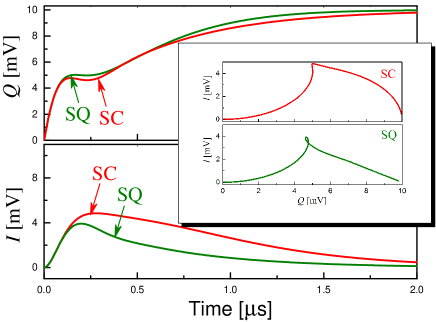
Figure 8: Time dependence of the quadratures calculated in semiclassical (SC) and semi-quantum (SQ) approximations, where upper panel presents $Q$ quadrature and lower panel presents $I$ quadrature. In the inset, dynamics of the quadratures is presented in the $IQ$ plane, where the upper panel presents the semiclassical approximation and the lower panel presents the semi-quantum calculations.

We consider the situation, when the qubit-resonator detuning $\Delta=\hbar\left(\omega_{\mathrm{q}}-\omega_{\mathrm{r}}\right)$ is much larger than the coupling strength $\mathrm{g}$, then the system is described by the dispersive approximation of the Jaynes-Cummings Hamiltonian Koch et al. (2007); Bianchetti et al. (2009)

$$H = \hbar(\omega_{\mathrm{r}}+\chi\sigma_{z})a^{{\dagger}}a+\hbar\frac{\omega_{\mathrm{q}}+\chi}{2}\sigma_{z}+$$ (35)

$$+\hbar\left(\xi a^{\dagger}e^{-i\omega t}+\frac{\Omega}{2}\sigma^{\dagger}e^{-i\omega_{\mathrm{d}}t}+h.c.\right).$$

Here the second line represents the two control fields. The full Hamiltonian $H$ of the system can be transformed with the operator $U=\exp[it(\omega a^{\dagger}a+\omega_{\mathrm{d}}\sigma_{z}/2)]$ to the following $H^{\prime}=UHU^{\dagger}+i\hbar\dot{U}U^{\dagger}$

$$H^{\prime} = \hbar(\delta\omega_{\mathrm{r}}+\chi\sigma_{z})a^{{\dagger}}a+\hbar\frac{\delta\omega_{\mathrm{q-d}}+\chi}{2}\sigma_{z}+$$ (36)

$$+\hbar\xi(a^{\dagger}+a)+\hbar\frac{\Omega}{2}(\sigma+\sigma^{\dagger}),$$

where $\delta\omega_{\mathrm{q-d}}=\omega_{\mathrm{q}}-\omega_{\mathrm{d}}$. Following Ref. [Bianchetti et al., 2009], now for the non-zero temperature, from the Lindblad equation (24), for the expectation values of the operators $\langle\sigma_{i}\rangle$ $(i=x,y,z)$ and the resonator field operators $\langle a\sigma_{i}\rangle$ and $\langle a^{\dagger}a\rangle$ we obtain the system of equations:

$$\frac{d}{dt}\langle\sigma_{z}\rangle\!\!\! = \!\!\!\Omega\langle\sigma_{y}\rangle-\Gamma_{1}\left(1+\frac{\langle\sigma_{z}\rangle}{z_{0}}\right),$$ (37a)

$$\frac{d}{dt}\langle\sigma_{x}\rangle\!\!\! = \!\!\!-\!\left(2\chi\!\!\left\langle a^{\dagger}a\right\rangle\!+\!\delta\omega_{\mathrm{q-d}}+\!\chi\right)\!\langle\sigma_{y}\rangle-\Gamma_{2}\!\frac{\langle\sigma_{x}\rangle}{z_{0}}\!,$$ (37b)

$$\frac{d}{dt}\langle\sigma_{y}\rangle\!\!\! = \!\!\!\left(2\chi\left\langle a^{\dagger}a\right\rangle+\delta\omega_{\mathrm{q-d}}+\chi\right)\langle\sigma_{x}\rangle-$$

$$-\Gamma_{2}\frac{\langle\sigma_{y}\rangle}{z_{0}}-\Omega\langle\sigma_{z}\rangle,$$

$$\frac{d}{dt}\langle a\rangle\!\!\! = \!\!\!-i\left(\delta\omega_{\mathrm{r}}\langle a\rangle+\chi\langle a\sigma_{z}\rangle+\xi\right)-\frac{\kappa}{2}\langle a\rangle,$$ (37d)

$$\frac{d}{dt}\langle a^{\dagger}a\rangle\!\!\! = \!\!\!-2\xi\text{\thinspace Im\thinspace}\langle a\rangle+\kappa\left(N_{\mathrm{th}}-\langle a^{\dagger}a\rangle\right),$$ (37e)

$$\frac{d}{dt}\langle a\sigma_{z}\rangle\!\!\! = \!\!\!-i\left(\delta\omega_{\mathrm{r}}\left\langle a\sigma_{z}\right\rangle+\chi\langle a\rangle+\xi\right)\langle\sigma_{z}\rangle+$$

$$+\Omega\langle a\sigma_{y}\rangle-\Gamma_{1}\left\langle a\right\rangle-\left(\frac{\Gamma_{1}}{z_{0}}+\frac{\kappa}{2}\right)\langle a\sigma_{z}\rangle,$$

$$\frac{d}{dt}\langle a\sigma_{x}\rangle\!\!\! = \!\!\!-i\delta\omega_{\mathrm{r}}\left\langle a\sigma_{x}\right\rangle-\left(\frac{\Gamma_{2}}{z_{0}}+\frac{\kappa}{2}\right)\langle a\sigma_{x}\rangle+$$

$$+\left(\delta\omega_{\mathrm{q-d}}+2\chi\left(\langle a^{\dagger}a\rangle+1\right)\right)\langle a\sigma_{y}\rangle-i\xi\langle\sigma_{x}\rangle,$$

$$\frac{d}{dt}\langle a\sigma_{y}\rangle\!\!\! = \!\!\!-i\delta\omega_{\mathrm{r}}\left\langle a\sigma_{y}\right\rangle-\left(\frac{\Gamma_{2}}{z_{0}}+\frac{\kappa}{2}\right)\langle a\sigma_{y}\rangle-$$ (37i)

$$-i\xi\langle\sigma_{y}\rangle-\Omega\langle a\sigma_{z}\rangle-$$

$$-\left(\delta\omega_{\mathrm{q-d}}+2\chi\left(\langle a^{\dagger}a\rangle+1\right)\right)\langle a\sigma_{x}\rangle.$$

Here we have truncated the infinite series of equations by factoring higher-order terms $\langle a^{\dagger}a\sigma_{i}\rangle\thickapprox\langle a^{\dagger}a\rangle\langle\sigma_{i}\rangle$ and $\langle a^{\dagger}aa\sigma_{i}\rangle\thickapprox\langle a^{\dagger}a\rangle\langle a\sigma_{i}\rangle$. Note that at $T=0$, the system (37) coincides with Eq. (5) in Ref. [Bianchetti et al., 2009].

We have numerically solved the system of equations (37) and the results are shown in Fig. 8. The two main panels present dynamics of the quadratures, where the red curves are the result of calculations in the semiclassical calculations, demonstrated in the main text in Fig. 1. The green curves present dynamics of the quadratures calculated in the semi-quantum approximation. There is a good quantitative agreement between the two approximations for the $Q$ quadrature, while the agreement for the $I$ quadrature during the transient stage is only qualitative. In addition, to further emphasize similarity and distinction of the two approaches, we present these quadratures in the inset in Fig. 8. While the two approaches give similar dynamics of the quadratures, the semiclassical approximation does not describe the self-crossing of the $IQ$ curve. Such dependence, including the self-crossing feature, was demonstrated in Fig. 4(d) of Ref. [Bianchetti et al., 2009]. We can make the conclusion here that the semiclassical calculations are good for obtaining analytical expressions, which describe qubit-resonator dynamics, while for describing some fine features of the dynamics, semi-quantum calculations may be necessary. Most importantly, we can see that the semiclassical calculations give correct values for the stationary variables.

Appendix C Quantum-to-classical transition for the strongly driven qubit-resonator system

In order to further demonstrate our approach, we devote this Section to the regime of strong driving of the qubit-resonator system. The frequency shift of the resonant transmission through the system was recently studied in detail in Refs. [Pietikäinen et al., 2017, 2018]. There, the authors studied such quantum-to-classical transition both experimentally and theoretically. Importantly, they have compared several numerical approaches, with RWA and without, taking into account both two transmon levels only and also higher levels. Our calculations are rather analytical and comparing them with the ones from Refs. [Pietikäinen et al., 2017, 2018] shows both applicability and limitations of our approach.

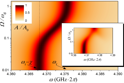
Figure 9: The resonant-frequency shift for the strongly-driven qubit-resonator system. The transmission amplitude $A$ is plotted as a function of the probing frequency $\omega$ and the driving amplitude $\Omega$ for the off-resonant driving with $\omega_{\mathrm{d}}\neq\omega_{\mathrm{q}}$. Semiclassical and semi-quantum calculations are presented in the main panel and in the inset, respectively.

So, for calculations we took the parameters close to the ones of Ref. [Pietikäinen et al., 2017]: $\omega_{\mathrm{r}}/2\pi=4.376$ GHz, $\omega_{\mathrm{q}}/2\pi=5.16$ GHz, $\mathrm{g}/2\pi=80~{}$MHz (which gives $\chi/2\pi=8.2$ MHz), $\varkappa/2\pi=4$ MHz, $\Gamma_{1}/2\pi=2$ MHz, $\Gamma_{2}=\Gamma_{1}$, and also driving frequency $\omega_{\mathrm{d}}=4.35$ GHz$\cdot 2\pi$. For this off-resonant driving ($\omega_{\mathrm{d}}\neq\omega_{\mathrm{q}}$) we make use of Eq. (13) and then, together with Eq. (7), we plot the transmission amplitude in the main panel in Fig. 9. This displays transition from the low-amplitude driving, when the resonant transmission appears around $\omega=\omega_{\mathrm{r}}-\chi$, corresponding to the qubit in the ground state, to the high-amplitude driving, when the qubit is in the superposition state, with average $P_{+}=1/2$ and the resonant transition appears around $\omega=\omega_{\mathrm{r}}$. One can observe that with increasing the driving amplitude $\Omega$, the frequency shifts by the value $\chi$, which is defined in Eq. (8), $\chi=\mathrm{g}_{0}^{2}E_{\mathrm{c}}/\Delta(\Delta-E_{\mathrm{c}})$. We must note that for the resonant driving, with $\omega_{\mathrm{d}}=\omega_{\mathrm{q}}$, it is much easier to saturate the qubit population and this happens at much smaller driving power, at $\Omega\sim 0.001\omega_{\mathrm{d}}\sim 2\sqrt{\Gamma_{1}\Gamma_{2}}$, rather than at $\Omega\sim\omega_{\mathrm{d}}$ in Fig. 9; it is thus non-resonant driving which allows consideration of the resonance shift in the regime of strong driving [Jerger et al., 2017].

In addition to the semiclassical calculations, in the inset in Fig. 9 we present the resonant-frequency shift in the semi-quantum approximation, for which we solved the system of equations (37). Overall, the shift of the resonance is consistent with the semiclassical calculations in the main part of Fig. 9; the suppression of the peak in the crossover region makes better resemblance with the experimental results and numerical calculations in Ref. [Pietikäinen et al., 2017].

References

- Koch et al. (2007) J. Koch, T. M. Yu, J. Gambetta, A. A. Houck, D. I. Schuster, J. Majer, A. Blais, M. H. Devoret, S. M. Girvin, and R. J. Schoelkopf, “Charge-insensitive qubit design derived from the Cooper pair box,” Phys. Rev. A 76, 042319 (2007).
- Ashhab and Nori (2010) S. Ashhab and F. Nori, “Qubit-oscillator systems in the ultrastrong-coupling regime and their potential for preparing nonclassical states,” Phys. Rev. A 81, 042311 (2010).
- Wendin (2017) G. Wendin, “Quantum information processing with superconducting circuits: a review,” Rep. Prog. Phys. 80, 106001 (2017).
- Giazotto et al. (2006) F. Giazotto, T. T. Heikkilä, A. Luukanen, A. M. Savin, and J. P. Pekola, “Opportunities for mesoscopics in thermometry and refrigeration: Physics and applications,” Rev. Mod. Phys. 78, 217–274 (2006).
- Albash et al. (2017) T. Albash, V. Martin-Mayor, and I. Hen, “Temperature scaling law for quantum annealing optimizers,” Phys. Rev. Lett. 119, 110502 (2017).
- Wilson et al. (2010) C. M. Wilson, G. Johansson, T. Duty, F. Persson, M. Sandberg, and P. Delsing, “Dressed relaxation and dephasing in a strongly driven two-level system,” Phys. Rev. B 81, 024520 (2010).
- Forn-Diaz et al. (2017) P. Forn-Diaz, J. J. Garcia-Ripoll, B. Peropadre, J.-L. Orgiazzi, M. A. Yurtalan, R. Belyansky, C. M. Wilson, and A. Lupascu, “Ultrastrong coupling of a single artificial atom to an electromagnetic continuum in the nonperturbative regime,” Nat. Phys. 13, 39 (2017).
- Stehlik et al. (2016) J. Stehlik, Y.-Y. Liu, C. Eichler, T. R. Hartke, X. Mi, M. J. Gullans, J. M. Taylor, and J. R. Petta, “Double quantum dot Floquet gain medium,” Phys. Rev. X 6, 041027 (2016).
- Palacios-Laloy et al. (2009) A. Palacios-Laloy, F. Mallet, F. Nguyen, F. Ong, P. Bertet, D. Vion, and D. Esteve, “Spectral measurement of the thermal excitation of a superconducting qubit,” Physica Scripta T137, 014015 (2009).
- Fink et al. (2010) J. M. Fink, L. Steffen, P. Studer, L. S. Bishop, M. Baur, R. Bianchetti, D. Bozyigit, C. Lang, S. Filipp, P. J. Leek, and A. Wallraff, “Quantum-to-classical transition in cavity quantum electrodynamics,” Phys. Rev. Lett. 105, 163601 (2010).
- Brunelli et al. (2011) M. Brunelli, S. Olivares, and M. G. A. Paris, “Qubit thermometry for micromechanical resonators,” Phys. Rev. A 84, 032105 (2011).
- Higgins et al. (2013) K. D. B. Higgins, B. W. Lovett, and E. M. Gauger, “Quantum thermometry using the ac Stark shift within the Rabi model,” Phys. Rev. B 88, 155409 (2013).
- Ashhab (2014) S. Ashhab, “Landau-Zener transitions in a two-level system coupled to a finite-temperature harmonic oscillator,” Phys. Rev. A 90, 062120 (2014).
- Jevtic et al. (2015) S. Jevtic, D. Newman, T. Rudolph, and T. M. Stace, “Single-qubit thermometry,” Phys. Rev. A 91, 012331 (2015).
- Ahmed et al. (2018) I. Ahmed, A. Chatterjee, S. Barraud, J. J. L. Morton, J. A. Haigh, and M. F. Gonzalez-Zalba, “Primary thermometry of a single reservoir using cyclic electron tunneling in a CMOS transistor,” arXiv:1805.03443 (2018).
- Mi et al. (2016) X. Mi, J. V. Cady, D. M. Zajac, P. W. Deelman, and J. R. Petta, “Strong coupling of a single electron in silicon to a microwave photon,” Science 355, 156–158 (2016).
- Bianchetti et al. (2009) R. Bianchetti, S. Filipp, M. Baur, J. M. Fink, M. Göppl, P. J. Leek, L. Steffen, A. Blais, and A. Wallraff, “Dynamics of dispersive single-qubit readout in circuit quantum electrodynamics,” Phys. Rev. A 80, 043840 (2009).
- Gong et al. (2016) M. Gong, Y. Zhou, D. Lan, Y. Fan, J. Pan, H. Yu, J. Chen, G. Sun, Y. Yu, S. Han, and P. Wu, “Landau-Zener-Stückelberg-Majorana interference in a 3D transmon driven by a chirped microwave,” Appl. Phys. Lett. 108, 112602 (2016).
- Remizov et al. (2017) S. V. Remizov, D. S. Shapiro, and A. N. Rubtsov, “Role of qubit-cavity entanglement for switching dynamics of quantum interfaces in superconductor metamaterials,” JETP Lett. 105, 130 (2017).
- Jin et al. (2015) X. Y. Jin, A. Kamal, A. P. Sears, T. Gudmundsen, D. Hover, J. Miloshi, R. Slattery, F. Yan, J. Yoder, T. P. Orlando, S. Gustavsson, and W. D. Oliver, “Thermal and residual excited-state population in a 3D transmon qubit,” Phys. Rev. Lett. 114, 240501 (2015).
- Pietikäinen et al. (2017) I. Pietikäinen, S. Danilin, K. S. Kumar, A. Vepsäläinen, D. S. Golubev, J. Tuorila, and G. S. Paraoanu, “Observation of the Bloch-Siegert shift in a driven quantum-to-classical transition,” Phys. Rev. B 96, 020501 (2017).
- Di Ventra et al. (2009) M. Di Ventra, Y. V. Pershin, and L. O. Chua, “Circuit elements with memory: Memristors, memcapacitors, and meminductors,” Proc. IEEE 97, 1717 (2009).
- Pershin and Di Ventra (2011) Y. V. Pershin and M. Di Ventra, “Memory effects in complex materials and nanoscale systems,” Adv. Phys. 60, 145 (2011).
- Peotta and Di Ventra (2014) S. Peotta and M. Di Ventra, “Superconducting memristors,” Phys. Rev. Applied 2, 034011 (2014).
- Guarcello et al. (2017a) C. Guarcello, P. Solinas, M. Di Ventra, and F. Giazotto, “Solitonic Josephson-based meminductive systems,” Sci. Rep. 7, 46736 (2017a).
- Guarcello et al. (2017b) C. Guarcello, P. Solinas, M. Di Ventra, and F. Giazotto, “Hysteretic superconducting heat-flux quantum modulator,” Phys. Rev. Applied 7, 044021 (2017b).
- Pfeiffer et al. (2016) P. Pfeiffer, I. L. Egusquiza, M. Di Ventra, M. Sanz, and E. Solano, “Quantum memristors,” Sci. Rep. 6, 29507 (2016).
- Shevchenko et al. (2016) S. N. Shevchenko, Y. V. Pershin, and F. Nori, “Qubit-based memcapacitors and meminductors,” Phys. Rev. Applied 6, 014006 (2016).
- Salmilehto et al. (2017) J. Salmilehto, F. Deppe, M. Di Ventra, M. Sanz, and E. Solano, “Quantum memristors with superconducting circuits,” Sci. Rep. 7, 42044 (2017).
- Li et al. (2017) Y. Li, G. W. Holloway, S. C. Benjamin, G. A. D. Briggs, J. Baugh, and J. A. Mol, “Double quantum dot memristor,” Phys. Rev. B 96, 075446 (2017).
- Sanz et al. (2017) M. Sanz, L. Lamata, and E. Solano, “Quantum memristors in quantum photonics,” arXiv:1709.07808 (2017).
- Bishop et al. (2009) L. S. Bishop, J. M. Chow, J. Koch, A. A. Houck, M. H. Devoret, E. Thuneberg, S. M. Girvin, and R. J. Schoelkopf, “Nonlinear response of the vacuum Rabi resonance,” Nat. Phys. 5, 105 (2009).
- Schleich (2001) W. P. Schleich, Quantum Optics in Phase Space (Wiley-VCH, Berlin, 2001).
- Shevchenko et al. (2014) S. N. Shevchenko, G. Oelsner, Y. S. Greenberg, P. Macha, D. S. Karpov, M. Grajcar, U. Hübner, A. N. Omelyanchouk, and E. Il’ichev, “Amplification and attenuation of a probe signal by doubly dressed states,” Phys. Rev. B 89, 184504 (2014).
- Mu and Savage (1992) Y. Mu and C. M. Savage, “One-atom lasers,” Phys. Rev. A 46, 5944–5954 (1992).
- Hauss et al. (2008) J. Hauss, A. Fedorov, S. André, V. Brosco, C. Hutter, R. Kothari, S. Yeshwanth, A. Shnirman, and G. Schön, “Dissipation in circuit quantum electrodynamics: lasing and cooling of a low-frequency oscillator,” New J. Phys. 10, 095018 (2008).
- André et al. (2009) S. André, V. Brosco, M. Marthaler, A. Shnirman, and G. Schön, “Few-qubit lasing in circuit QED,” Physica Scripta T137, 014016 (2009).
- Macha et al. (2014) P. Macha, G. Oelsner, J.-M. Reiner, M. Marthaler, S. André, G. Schön, U. Hübner, H.-G. Meyer, E. Il’ichev, and A. V. Ustinov, “Implementation of a quantum metamaterial using superconducting qubits,” Nature Comm. 5, 5146 (2014).
- Bianchetti (2010) R. A. Bianchetti, “Control and readout of a superconducting artificial atom,” PhD Thesis, ETH Zurich (2010).
- Reed et al. (2010) M. D. Reed, L. DiCarlo, B. R. Johnson, L. Sun, D. I. Schuster, L. Frunzio, and R. J. Schoelkopf, “High-fidelity readout in circuit quantum electrodynamics using the Jaynes-Cummings nonlinearity,” Phys. Rev. Lett. 105, 173601 (2010).
- Jerger et al. (2016a) M. Jerger, P. Macha, A. R. Hamann, Y. Reshitnyk, K. Juliusson, and A. Fedorov, “Realization of a binary-outcome projection measurement of a three-level superconducting quantum system,” Phys. Rev. Applied 6, 014014 (2016a).
- Jerger et al. (2016b) M. Jerger, Y. Reshitnyk, M. Oppliger, A. Potocnik, M. Mondal, A. Wallraff, K. Goodenough, S. Wehner, K. Juliusson, N. K. Langford, and A. Fedorov, “Contextuality without nonlocality in a superconducting quantum system,” Nature Comm. 7, 12930 (2016b).
- Reagor et al. (2016) M. Reagor, W. Pfaff, C. Axline, R. W. Heeres, N. Ofek, K. Sliwa, E. Holland, C. Wang, J. Blumoff, K. Chou, M. J. Hatridge, L. Frunzio, M. H. Devoret, L. Jiang, and R. J. Schoelkopf, “Quantum memory with millisecond coherence in circuit QED,” Phys. Rev. B 94, 014506 (2016).
- Vijay et al. (2011) R. Vijay, D. H. Slichter, and I. Siddiqi, “Observation of quantum jumps in a superconducting artificial atom,” Phys. Rev. Lett. 106, 110502 (2011).
- Filipp et al. (2009) S. Filipp, P. Maurer, P. J. Leek, M. Baur, R. Bianchetti, J. M. Fink, M. Göppl, L. Steffen, J. M. Gambetta, A. Blais, and A. Wallraff, “Two-qubit state tomography using a joint dispersive readout,” Phys. Rev. Lett. 102, 200402 (2009).
- McClure et al. (2016) D. T. McClure, H. Paik, L. S. Bishop, M. Steffen, J. M. Chow, and J. M. Gambetta, “Rapid driven reset of a qubit readout resonator,” Phys. Rev. Applied 5, 011001 (2016).
- Jerger et al. (2017) M. Jerger, Z. Vasselin, and A. Fedorov, “In situ characterization of qubit control lines: a qubit as a vector network analyzer,” arXiv:1706.05829 (2017).
- Lu et al. (2017) X. J. Lu, M. Li, Z. Y. Zhao, C. L. Zhang, H. P. Han, Z. B. Feng, and Y. Q. Zhou, “Nonleaky and accelerated population transfer in a transmon qutrit,” Phys. Rev. A 96, 023843 (2017).
- Dai et al. (2017) K. Dai, H. Wu, P. Zhao, M. Li, Q. Liu, G. Xue, X. Tan, H. Yu, and Y. Yu, “Quantum simulation of general semi-classical Rabi model beyond strong driving regime,” Appl. Phys. Lett. 111, 242601 (2017).
- Peterer et al. (2015) M. J. Peterer, S. J. Bader, X. Jin, F. Yan, A. Kamal, T. J. Gudmundsen, P. J. Leek, T. P. Orlando, W. D. Oliver, and S. Gustavsson, “Coherence and decay of higher energy levels of a superconducting transmon qubit,” Phys. Rev. Lett. 114, 010501 (2015).
- Pietikäinen et al. (2018) I. Pietikäinen, S. Danilin, K. S. Kumar, J. Tuorila, and G. S. Paraoanu, “Multilevel effects in a driven generalized Rabi model,” J. Low. Temp. Phys. (2018).
- Scully and Zubairy (1997) M. O. Scully and M. S. Zubairy, Quantum Optics (Cambridge, Cambridge University Press, 1997).